Infrasound measurement system for real-time in situ tornado measurements

Previous work suggests that acoustic waves at frequencies below human hearing (infrasound) are produced during tornadogenesis and continue through the life of a tornado, which have potential to locate and profile tornadic events and provide a range of improvements relative to current radar capabilities, which are the current primary measurement tool. Confirming and identifying the fluid mechanism responsible for infrasonic production has been impeded by limited availability and quality (propagation-related uncertainty) of tornadic infrasound data. This paper describes an effort to increase the number of measurements and reduce the uncertainty in subsequent analysis by equipping storm chasers and first responders in regular proximity to tornadoes with mobile infrasound measurement capabilities. The study focus is the design, calibration, deployment, and analysis of data collected by a Ground-based Local INfrasound Data Acquisition (GLINDA) system that collects and relays data from an infrasound microphone, GPS receiver, and an inertial measurement unit (IMU). GLINDA has been deployed with storm chasers beginning in May 2020 and has provided continuing real-time automated monitoring of spectrum and peak detection. In analysis of sampled severe weather phenomena, the signal measured from an EFU (EF-Unknown, where EF represents the Enhanced Fujita scale) tornado (Lakin, KS, USA) shows an elevated broadband signal between 10 and 15 Hz. A significant hail event produced no significant increase in infrasound signal despite rotation in the storm. The consistency of these observations with existing fixed-array measurements and real-time tools to reduce measurement uncertainty demonstrates the value of acquiring tornado infrasound observations from mobile on-location systems and introduces a capability for real-time processing and display of mobile infrasonic measurements.

1 Introduction

Tornadoes remain a significant hazard to life and property. In the United States, 800–1400 annually reported tornadoes claim an average of 55 lives (Ashley, 2007; Paul and Stimers, 2012) with 76 confirmed fatalities in the United States in 2020 (NOAA/SPC, 2021). Many fatalities occur in the southeast United States due, in part, to hilly terrain limiting line-of-sight measurements (such as radar) and radar horizon interactions. This has motivated a search for alternative methods to complement radar measurements. Infrasound, sound below human hearing (< 20 Hz), is one possibility. Infrasound in the nominal range of 0.5 to 10 Hz has been observed coming from the same region as tornadoes that were verified with Doppler radar and/or visual observations (Bedard et al., 2004b, a; Frazier et al., 2014; Goudeau et al., 2018; Elbing et al., 2019). These recent observations suggest that the infrasound signal may carry information specific to the tornado structure and dynamics. Since infrasound can be detected over long distances due to weak atmospheric absorption at these frequencies, it is a potential means of long-range, passive tornado monitoring.

Table 1 Infrasound has several potential advantages over existing weather radar measurements as a potential mechanism for tornado detection and tracking.

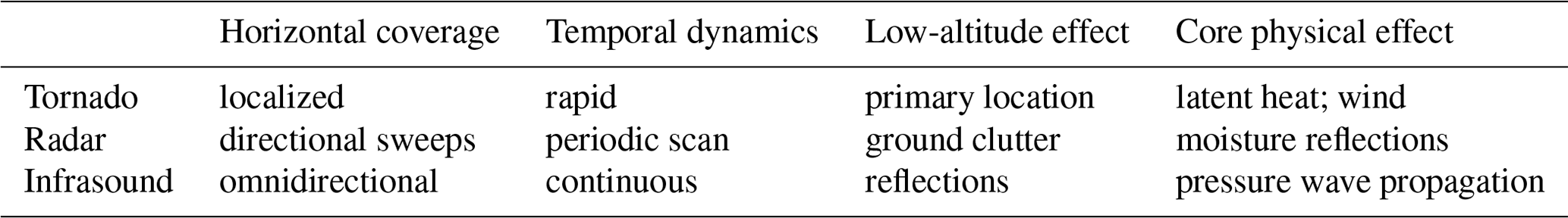
Table 1 provides a comparison between aspects of infrasound measurements and the respective properties as observed in the tornado dynamics and radar measurement. The long propagation range of infrasound, coupled with the omnidirectional, continuous coverage provided by relatively inexpensive infrasound microphones, could provide a significant improvement in our ability to detect, track, and ultimately predict and understand tornadic phenomena. However, the limited availability and quality of tornado-relevant infrasound measurement systems, coupled with the required development effort, have inhibited the integration of these measurements into a national framework. In this work, we introduce a portable infrasound measurement tool that may be carried by storm chasers and first responders, combined with a real-time interface portal. These are the first tools available to the public that are applicable to mobile deployment and would provide widespread real-time infrasound coverage near the bases of tornadoes without additional cost to the end user.

2 Previous work and background

The tornado-infrasound production hypothesis first appeared in 1960s' conferences, and only a minority of early work is available in archival journals (Georges, 1973). Contemporary tornado infrasound results continue to be reported primarily in conference papers (Noble and Tenney, 2003; Bedard et al., 2004b, a; Prassner and Noble, 2004), project reports (Rinehart, 2018), and oral presentations (Rinehart, 2012; Goudeau et al., 2018). Exceptions to this trend include four journal articles focused on infrasound observations from tornadoes (Bedard, 2005; Frazier et al., 2014; Dunn et al., 2016; Elbing et al., 2019). Bedard (2005) showed that infrasound emissions of ≈ 1 Hz followed the available radar observations associated with a tornado. Bedard (2005) also indicates that over 100 infrasound signals from the NOAA Infrasound Network (ISNET) were determined to be associated with tornado and tornado formation processes; the details of the association technique are not included in the article. Frazier et al. (2014) tracked tornadoes in Oklahoma using beamforming at infrasound frequencies. Dunn et al. (2016) report on a set of four tornado-producing storms in which a 0.94 Hz acoustic signature was detected and associated with an EF4 (where EF represents the Enhanced Fujita scale) tornado in Arkansas using a ring laser interferometer. This signal “was initially observed 30 [min] before the funnel was reported on the ground”.

Systematic infrasound observations from tornadoes and their formation processes remain a research challenge, which continues to contribute to large uncertainties associated with the observations and the underlying fluid mechanism responsible for its production (Petrin and Elbing, 2019). The need for detailed tornado-related infrasound observations appropriate for archival literature motivated an effort to increase both the number and quality of tornado infrasound observations, beginning with the 2016 installation of a fixed, three-microphone infrasound array on the Oklahoma State University (OSU) campus. The OSU fixed-array observations have provided some of the most recent and complete tornadic infrasound measurements, including signals associated with the 11 May 2017 EFU tornado (Elbing et al., 2019). The fixed nature of this array limited the proximity to tornadoes and radar sites, and though 2019 included a historically high number of tornadoes (NOAA, 2020c), no 2019 observations had both reliable infrasound and radar data. To address this gap, a mobile, four-microphone infrasound array was developed (Petrin et al., 2020), heliotrope solar hot-air balloons (Bowman et al., 2020) were equipped with infrasound sensors (Vance et al., 2020), and a Ground-based Local INfrasound Data Acquisition (GLINDA) system was developed during 2019–2020 to be carried by storm chasers and first responders. The result is a robust ecosystem of complementary measurement technologies that are capable of improving the number and quality of infrasound measurements near tornadoes.

This paper focuses on the design, deployment, and recent results from the mobile storm-chasing unit (GLINDA). This unit provides a tool to mitigate uncertainties associated with atmospheric propagation by acquiring targeted close-range measurements from verified tornadoes. The GLINDA unit was deployed with storm chasers beginning in the 2020 tornado season, and it continues to provide valuable real-time measurements available through a web interface accessible to storm chasers and other meteorology partners.

This paper is organized as follows. Section 3 outlines the design goals, design process, and calibration procedure for the GLINDA unit. Section 4 covers the real-time processing needs and an automated analysis approach including variance reduction and peak quantification. Section 5 describes two example storm measurements (a tornado and hail-producing storm) recorded by the unit during the 2020 storm season and used to verify its operation. Section 6 shows calibration, spectral, and peak identification results for the installed unit and the example storms.

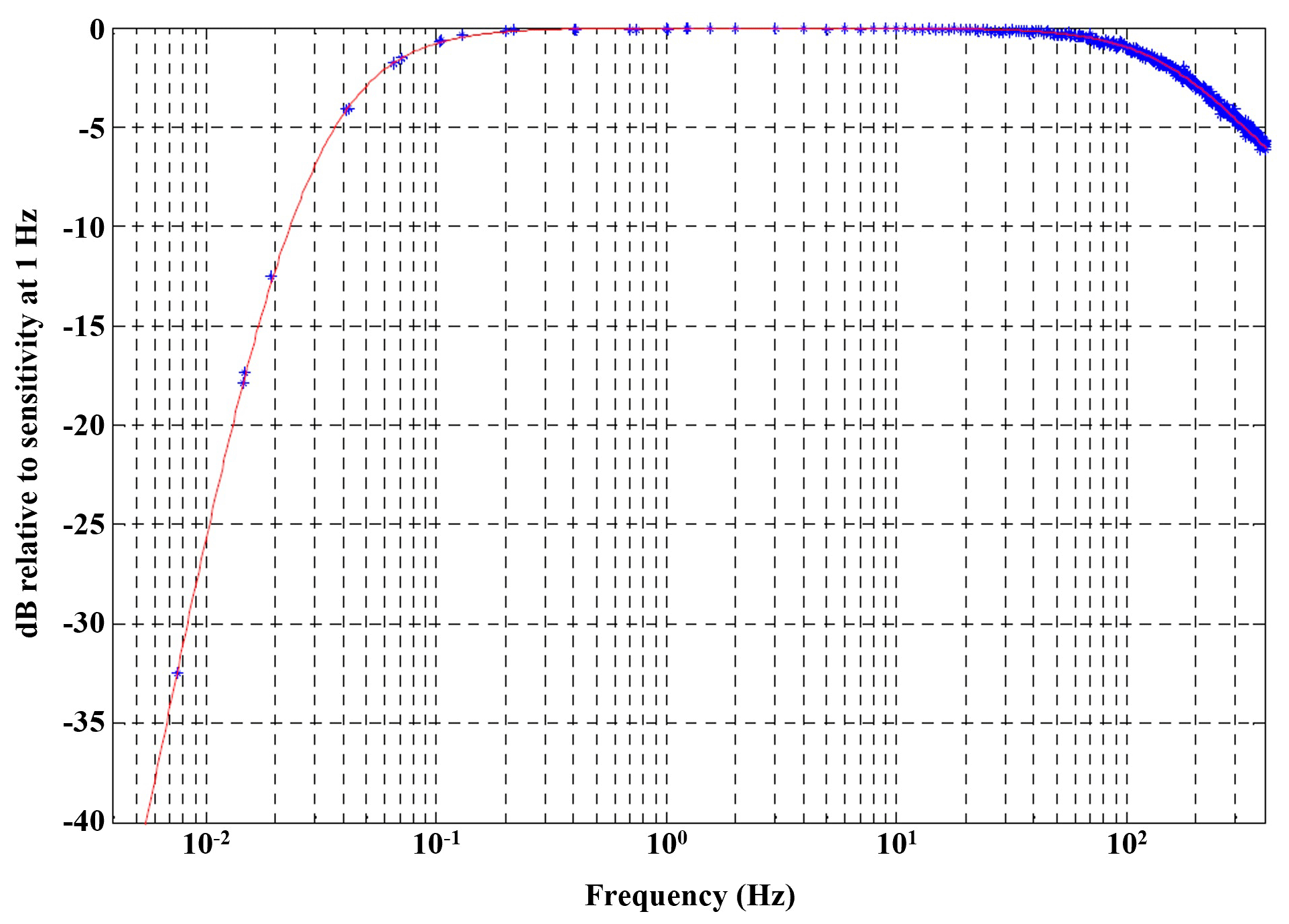
Figure 1 Typical frequency response curve for a model 24 (Chaparral Physics) microphone, which was used for this deployment of GLINDA. Credit: Chaparral Physics.

3 GLINDA design and calibration

In this section, system design goals are identified, and hardware components, computational platforms, and data handling for collection and retention prior to analysis are discussed. Additionally, calibration procedures over the specific range of frequencies of interests are presented for the unit.

3.1 System design

The primary measurement system goals were the following: (a) microphone signal resolution of 20 mPa or better to provide comparable infrasound feature resolution to existing fixed arrays (Elbing et al., 2019), (b) positioning resolution under 10 m to provide comparable or better precision to current NOAA-reported tornado coordinates (the United States National Weather Service, NWS, does not provide uncertainty or accuracy estimates for this number that would quantify accuracy), and (c) “real-time” remote data relay, where real time is defined as at or exceeding weather radar update frequencies (approximately once per 90 s).

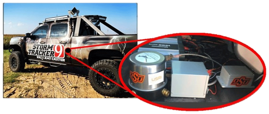
Figure 2 Image of the GLINDA-housing storm-chasing vehicle showing approximate location and configuration of install.

3.1.1 Infrasound microphone

GLINDA uses an off-the-shelf infrasound microphone (model 24, Chaparral Physics), which is the same model used for the fixed three-microphone array near Oklahoma State University (Elbing et al., 2019). The microphone has a sensitivity of 401 mV Pa⁻¹ at 1 Hz and a flat response from 0.1–200 Hz to within −3 dB (flat to within −0.5 dB for 0.3 to 50 Hz). The typical frequency response for this model of microphone is provided in Fig. 1. The noise for this microphone at 1 Hz was −81.6 dB relative to 1 Pa² Hz⁻¹. The microphone was mounted on the floorboard of the storm-chasing truck as shown in Fig. 2. Concerns about the ability to suppress wind noise motivated the mounting inside of the truck cab; consequently, no additional windscreen was implemented. The maximum signal output for the microphone was 36 V peak-to-peak, and the analog output signal was sampled at 2050 Hz. By sampling at greater than 2000 Hz, GLINDA avoids aliasing in the frequency band of interest.

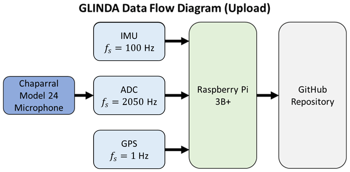
3.1.2 Sensor components

In addition to the infrasound microphone, GLINDA monitors and records data from an inertial measurement unit (IMU), a Global Positioning System (GPS) receiver, and the analog-to-digital converter (ADC) that was connected to the analog output from the infrasound microphone. An illustration of data flow for the upload process from each of the sensors is provided in Fig. 3. The IMU, GPS, and ADC were sampled at 100, 1, and 2050 Hz, respectively. The microphone ADC (ADS1115, Adafruit Industries) has a 16 bit resolution and signal voltage tolerance of ± 5 V, giving a quantization increment of 76 µV. Since the microphone outputs a differential signal reading of 0–36 V, a voltage divider circuit was implemented with gain ratio of 13.6 % to ensure the measured signals fall within the ADC tolerance. The nominal microphone sensitivity of 400 mV Pa⁻¹ provides a pressure resolution of 1.4 mPa, keeping GLINDA's quantization error below the existing fixed array's typical noise floor of 20 mPa observed during severe storms with high winds (Elbing et al., 2019). The GPS unit (746 Ultimate GPS Breakout Ver 3, Adafruit Industries) provides accuracy values of 1.8 m and 0.1 m s⁻¹. The value of 1.8 m radially is accurate to approximately 0.00001^∘ for data collection latitudes. For comparison, current NOAA tornado reports typically provide GPS coordinates with three to four decimals, and the system positioning accuracy exceeds these estimates. Each measurement is time-stamped and stored locally until export processes are initiated.

Figure 3 Flowchart for acquiring and uploading of data from GLINDA.

3.1.3 Computing platform

The mobile GLINDA hardware is built on a Raspberry Pi 3B+ platform with a Raspbian distribution. The scripts were written in Python 3.7 and implement Adafruit libraries for reading the attached sensor packages over I²C and serial/UART connections. Upon startup, the system initializes all sensors for data collection and continues recording until loss of power. Data are saved every 10 s to ensure minimal loss in the event of unexpected shutdown. Each data file is time-stamped by the local system time coordinated via Network Time Protocol thorough the Pi board. A system service initializes and maintains data uploads to a GitHub repository.

3.1.4 Installation and deployment

For the 2020 tornado season, GLINDA measured from within the cab of a storm-chasing truck operated by Val and Amy Castor (see Fig. 2), which provided live coverage of severe storms for a local news station in Oklahoma City, OK (News 9). GLINDA was installed during the first week of May 2020. It was powered by 1500 W inverters (Strongway), which also power the vehicle's other weather observation systems. The 60 Hz signal produced by the inverters is outside of the frequency band of interest. A small port in the roof of the vehicle allowed the GPS antenna to be routed outside of the cab for improved connectivity. Data size is limited by a power switch integrated into the vehicle dash.

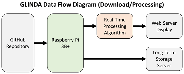
3.1.5 Data recovery

An illustration of the data flow from download through processing is provided in Fig. 4. GLINDA maintains an internet connection via a router in the storm-chasing vehicle that is primarily used to provide live video and audio to the local news outlet during storm chases. While connected to the internet, GLINDA scans the data storage directory for new or modified files resulting from sampling of the sensor packages. An upload commit is generated to push new or updated files to the online repository (GitHub). File uploads for the system are conducted at regular intervals, typically at Δt < 60 s. Further discussion on selection for timing considerations is provided in Sect. 3.1.

Figure 4 Data flow diagram for processing, display, and storage.

3.2 Calibration

To create a broadband acoustic and infrasound signal with sufficient excitation energy over the frequency bandwidth of interest, the GLINDA system was calibrated utilizing a series of impulsive acoustic signals generated from a 20-gauge shotgun discharged at < 2 ft (<1 m) range and oriented approximately 120^∘ from the unit installed in the vehicle model cabin (2019 Ford F-150). A gunshot was used to generate the impulsive signals of the test to generate significant acoustic and infrasonic spectra with similar magnitude. Two series of three gunshots were completed in cabin configurations of windows up and windows down. The gunshots from each configuration were then compiled into a single data series for frequency-domain analysis using approximately 1 s sections of recording containing each shot (approximately 0.1 s ringing). By comparing the signal measured outside of the vehicle to the interior microphone signal, an experimental transfer function was identified for the acoustic impact of the vehicle over the frequency band of interest. A frequency-domain model fit to the magnitude measurements was used as the transfer functions for the window up and window down cases.

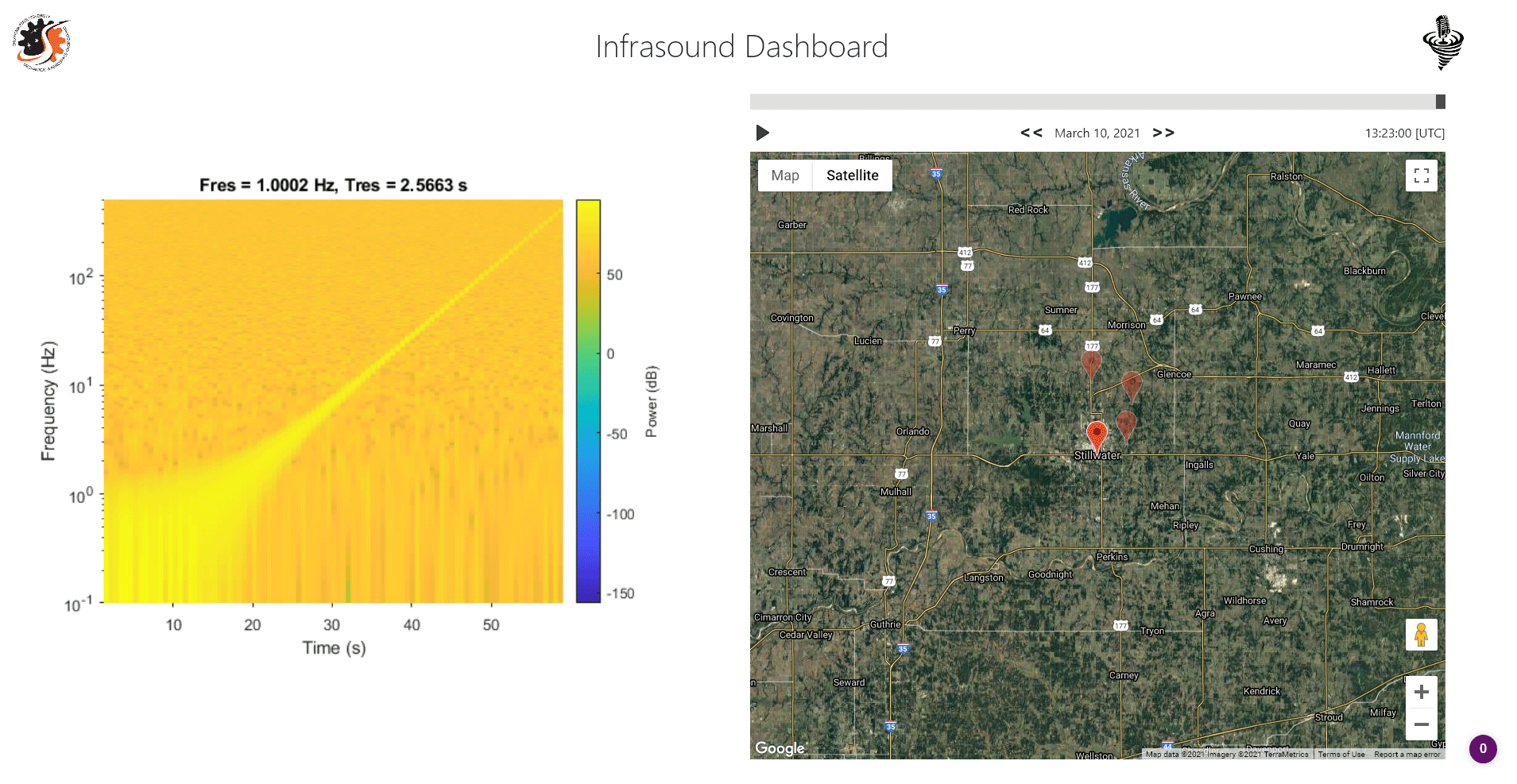
Figure 5 Example visualization of the GLINDA-monitoring web interface (see map graphic for copyright).

3.3 Real-time display interface

To provide continuous monitoring and rapidly identify temporal trends in acoustic measurements, allowing storm chasers to include infrasound signals in tactical decision-making, a web interface was developed that displays the GLINDA measurements in near real time. The primary visualizations of the data are a spectrogram displaying near-real-time frequency decompositions and a map API displaying the location of the storm-chasing unit via GPS. Figure 5 shows a demonstration of these visualization capabilities with simulated inputs. In the spectrogram, F_res and T_res represent the size of the frequency and time bins, respectively. In addition to visualizing current measurements, a slider for time and date allows for browsing historical data.

4 Analysis approach

In this section, a real-time analysis approach is developed that provides high-resolution spectral measurements over the region of interest and provides robust peak-detection and finding routines.

4.1 Real-time processing qualifications

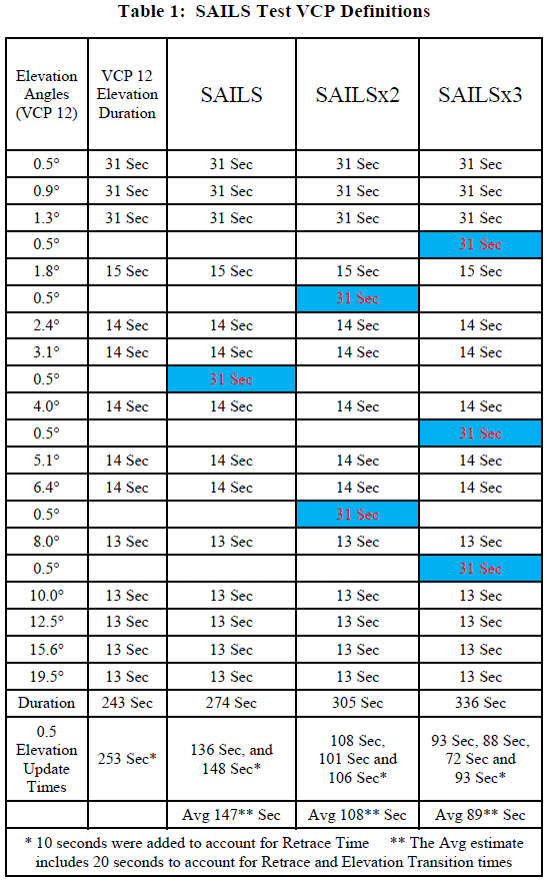
Traditional weather monitoring of severe weather, such as tornadoes in the United States, is completed via radar analysis. The United States National Weather Service (NWS) utilizes a widespread network of weather radars (most notably weather surveillance radar, 1988 Doppler, or WSR-88D) to provide the most accurate and frequent images available (US-NWS, 2017). Development of scanning methods that decrease time intervals between low-angle atmospheric sweeps for the WSR-88D have been the subject of repeated study and implementation (Daniel et al., 2014). The current methodology for minimizing the interval between scans is the Multiple Elevation Scan Option Supplemental Adaptive Intra-Volume Low-Level Scan or MESO-SAILS. The average time between MESO-SAILS scans at the 0.5^∘ radar inclination is provided in Table 2 and implies that GLINDA should target measurement intervals of ΔT_m≤ 90 s to be comparable with current radar technology.

Table 2 Average minimum wait time between low-inclination update scans for varieties of WSR-88D scanning methods.

The > 90 s update rate, data generation rate, and desired bandwidth usage is used to identify the maximum length of an individual recorded segment that keeps pace with radar as

$$\begin{array}{}\text{(1)}& \mathrm{89}\ge \mathrm{\Delta }{T}_{\mathrm{t}}=\mathrm{\Delta }{T}_{\mathrm{m}}+\mathrm{\Delta }{T}_{\mathrm{u}}={\displaystyle \frac{R_{\mathrm{G}}\mathrm{\Delta }{T}_{\mathrm{m}}}{\mathrm{0.1}{R}_{\mathrm{u}}}}+\mathrm{\Delta }{T}_{\mathrm{m}},\end{array}$$

where R_G is the rate of sensor data production, R_u is the minimum connection speed expected, total time between measurements (ΔT_t) is the sum of the time interval of data collection and the time required to upload the data (ΔT_u), and GLINDA data usage is limited to less than 10 % of the available bandwidth. For the GLINDA unit, R_G = 70 kB s⁻¹, and the upload constraint is 1.35ΔT_m≤ 89 s.

4.2 Spectral transformation

In 2020, GLINDA recorded several chases during severe weather events, including a dust storm, gustnado, and significant hail events. This paper analyzes the data acquired during a tornado-producing supercell including tornadogenesis and a severe hail event without tornadic activity. Traditionally the frequency decomposition of a time-domain signal is performed using a fast Fourier transform (FFT) which returns a frequency-domain representation of the data with linearly spaced frequency points over the frequency band $f_{\text{FFT}}\in [\mathrm{0},f_{\mathrm{s}}/\mathrm{2}]$, where $f_{\mathrm{s}}/\mathrm{2}$ is commonly known as the Nyquist frequency. For the oversampled case, a large number of these points would be outside the frequency band of interest. In this study, we used the oversampling to reduce the frequency-domain error by implementing a chirp Z-transform (CZT) to allow the frequency-domain resolution to be directed only across a desired frequency band (, ), which is advantageous, because the frequency band of interest for the current work is a relatively small fraction of the band returned by the FFT (≤ 10 %). Thus the CZT produces higher resolution over the desired range relative to an FFT. The CZT also has the advantage of reducing the required processing time, given the narrowed band, which is critical for enabling real-time analysis of infrasound measurements. However, due to the data sizes presented in the current study, the CZT and FFT had negligible runtime differences. The CZT, defined in Eq. (2), takes a time-domain series of N points, x(n), and transforms it into the complex Z-domain at a finite number of points along a defined spiral contour z(k) returning frequency-domain signal, X(k). Here z(k) is a function of a complex starting point A, the complex ratio between points W, and the number of spiral contour points M. For storm analyses over expected frequency bands previously associated with tornadic acoustics, a complex spiral was defined as given in Eq. (3), which corresponds to a band of 1–250 Hz with a frequency resolution of Δf = 0.125 Hz. A 10 min selection of microphone data was selected from 1 h before the event, spanning the event, and 1 h after the event for each case presented. The 10 min intervals were windowed using Hanning windows with 60 % overlap and segmented into 15 s lengths.

$$\begin{array}{}\text{(2)}& {\displaystyle }\begin{array}{rl}& X\left(k\right)=\sum _{n=\mathrm{0}}^{N-\mathrm{1}}x\left(n\right)z(k{)}^{-n},z(k)=A{W}^{-k},\\ & k=\mathrm{0},\mathrm{1},\mathrm{\dots },M-\mathrm{1};\end{array}\text{(3)}& {\displaystyle }\begin{array}{rl}& A=e^{\mathrm{2}\mathit{\pi }i/\mathrm{1000}},W=e^{(\mathrm{2}\mathit{\pi }/\mathrm{1000})(\mathrm{249}/\mathrm{2000})i},\\ & M=\mathrm{2000}.\end{array}\end{array}$$

4.3 Peak identification

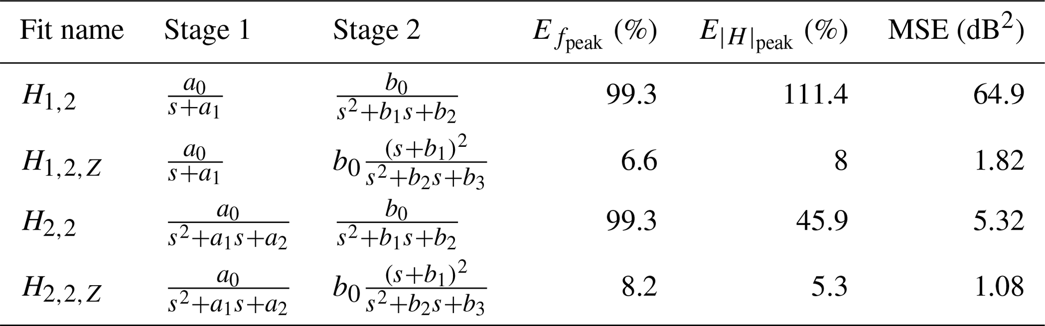
To robustly identify the frequency-domain peak in real time, a model-based approach was taken, using a two-stage process to compare fits to the four frequency-domain model structures shown in Fig. 6.

Figure 6 Frequency-domain model structures considered and two-stage model fitting process.

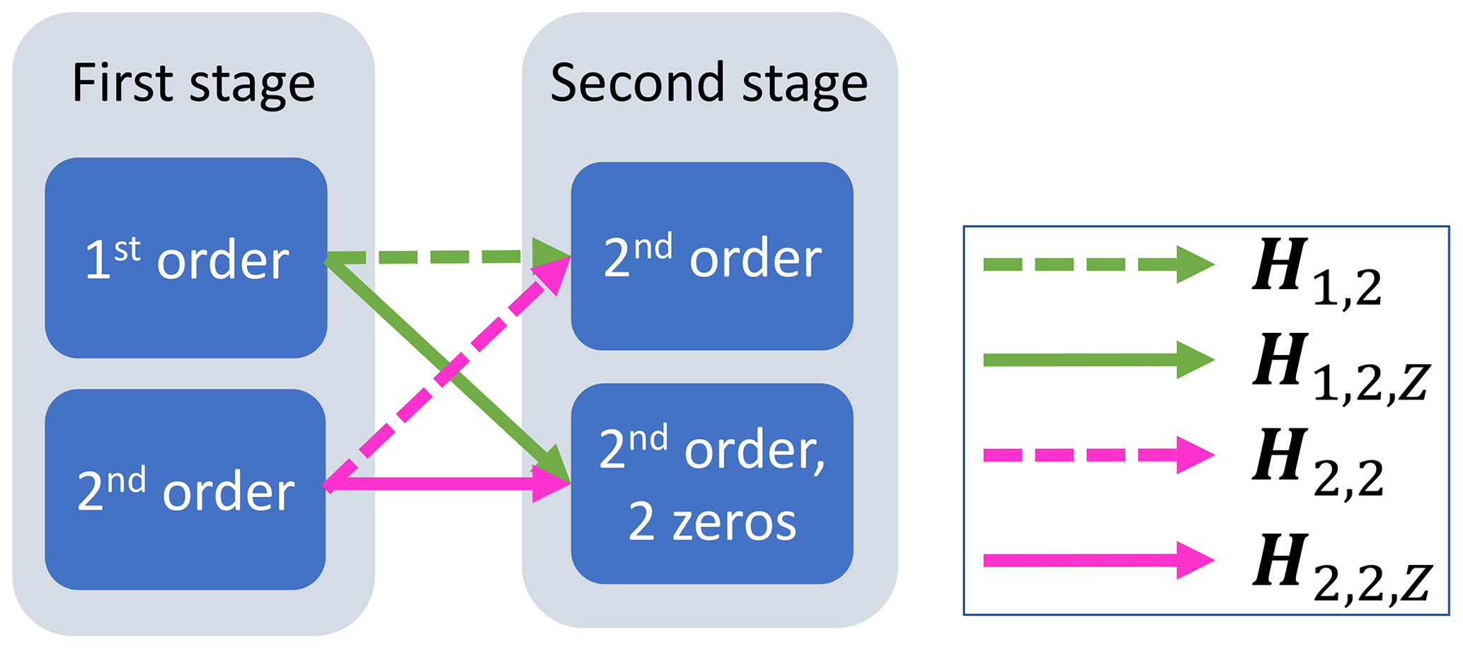
Each fit was derived by minimizing the mean-squared error (MSE) between the measured SPL ($\widehat{Y}$, sound pressure level) and frequency response magnitude of the transfer function (|H|) as Eq. (4).

$$\begin{array}{}\text{(4)}& \text{MSE}=\sum _{f=\mathrm{0.1}\mathrm{Hz}}^{\mathrm{100}\mathrm{Hz}}\left(\widehat{Y}\right(f)-\mathrm{|}H\mathrm{|}(f){)}^{\mathrm{2}}\end{array}$$

5 Observations

In this section, two significant weather events measured by GLINDA during the Spring 2020 tornado season are described. These weather events will be utilized as examples of the detailed analysis capable through the GLINDA system described in Sect. 4 with results presented in Sect. 6.

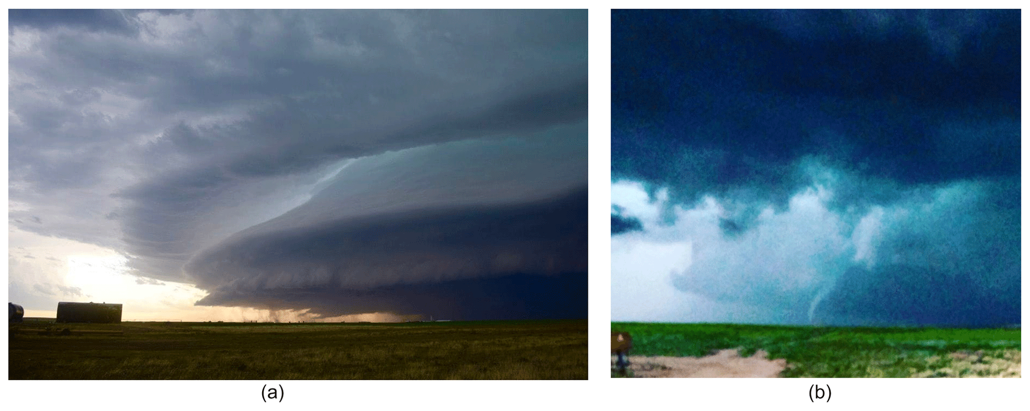
Figure 7 (a) Picture of the storm system that produced the tornado near Lakin, KS, on 22 May 2020. (b) Picture of the Lakin, KS, tornado. Photo credit: Val and Amy Castor.

5.1 Tornado event (22 May 2020)

A cold front that pushed in from the northwest of Kansas late on 21 May 2020 and into the early hours of 22 May 2020 produced several severe storms. One storm, pictured in Fig. 7, produced a tornado near Lakin, Kansas. The tornado formed at 00:11 UTC at NWS-reported coordinates (37.802, −101.468) and ended at 00:24 UTC at NWS-reported coordinates (37.7982, −101.4387). It was 2.83 km (1.76 miles) in length, had a maximum damage path width of 137 m (150 yd), and was classified as an EFU by the NWS, because it tracked over an open field that produced insufficient recorded damage for reliable categorization (NOAA, 2020b). The storm chasers, equipped with GLINDA, arrived to the intercepting location for the tornadic storm system approximately 2–5 min prior to tornado formation. The intercepting storm chasers were located approximately 4 km SSE of the tornado during tornado formation. Local radar and radial velocity data for this storm are provided in Appendix B.

5.2 Large hail (22 May 2020)

The day after the Lakin EFU tornado, a stalled outflow boundary intersected a dry line resulting in the firing of numerous severe thunderstorms. One of these large supercell storms produced baseball-sized hail as it moved over southern Oklahoma. The GLINDA-equipped storm chasers intercepted the storm as it moved through Comanche County and produced 25.4 mm (1 in.) hail at 23:15 UTC on 22 May 2020 near the NWS-reported coordinates (34.62, −98.75) (NOAA, 2020a). Of note, this storm did exhibit weak rotation at times, but a tornado was never produced.

6 Results and discussion

In this section, the calibration results are presented, the frequency-domain analyses of the two storms are compared, and the peak finding routine is applied to signals with an infrasound rise. The spectral comparison shows a rise in infrasonic signals in the presence of a tornado-producing supercell near tornadogenesis. The rise is statistically significant with respect to the signal noise and standard deviation, and it does not appear after the tornado or in a non-tornadic hail storm which contained rotation.

6.1 Calibration

Figure 9 provides the measured frequency response as obtained through calibration described in Sect. 3.2 for windows up and windows down configurations. A frequency-domain model fit to the magnitude measurements then gives transfer functions H_u(s) and H_d(s) for the window up and window down cases (Eqs. 5 and 6), respectively. These transfer functions are compared in Fig. 9.

$$\begin{array}{}\text{(5)}& {\displaystyle }{H}_{\mathrm{u}}={\displaystyle \frac{\mathrm{0.22}(s+\mathrm{31.5}{)}^{\mathrm{2}}}{(s+\mathrm{377}{)}^{\mathrm{2}}}},\text{(6)}& {\displaystyle }{H}_{\mathrm{d}}={\displaystyle \frac{\mathrm{0.79}(s+\mathrm{18.8}{)}^{\mathrm{2}}}{(s+\mathrm{471}{)}^{\mathrm{2}}}}.\end{array}$$

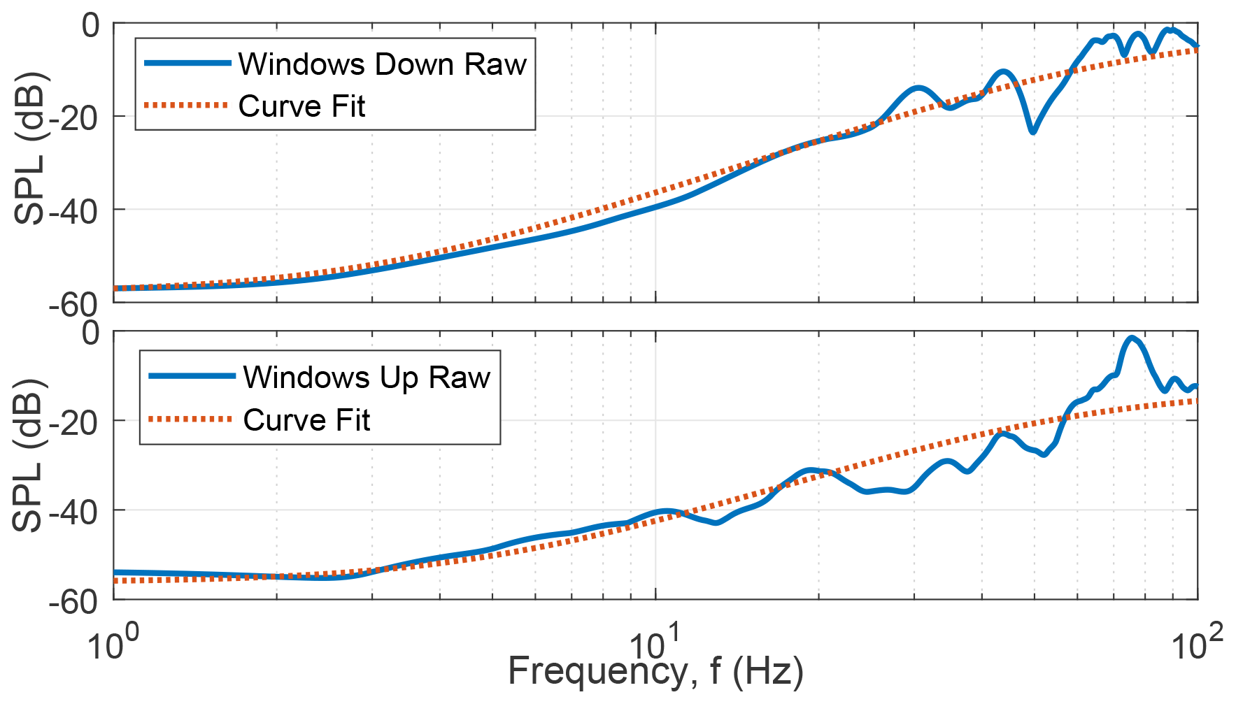
Figure 8 Experimental transfer function data and fitted models for windows up and windows down configurations.

Figure 9 Comparison of models for windows up and windows down configurations.

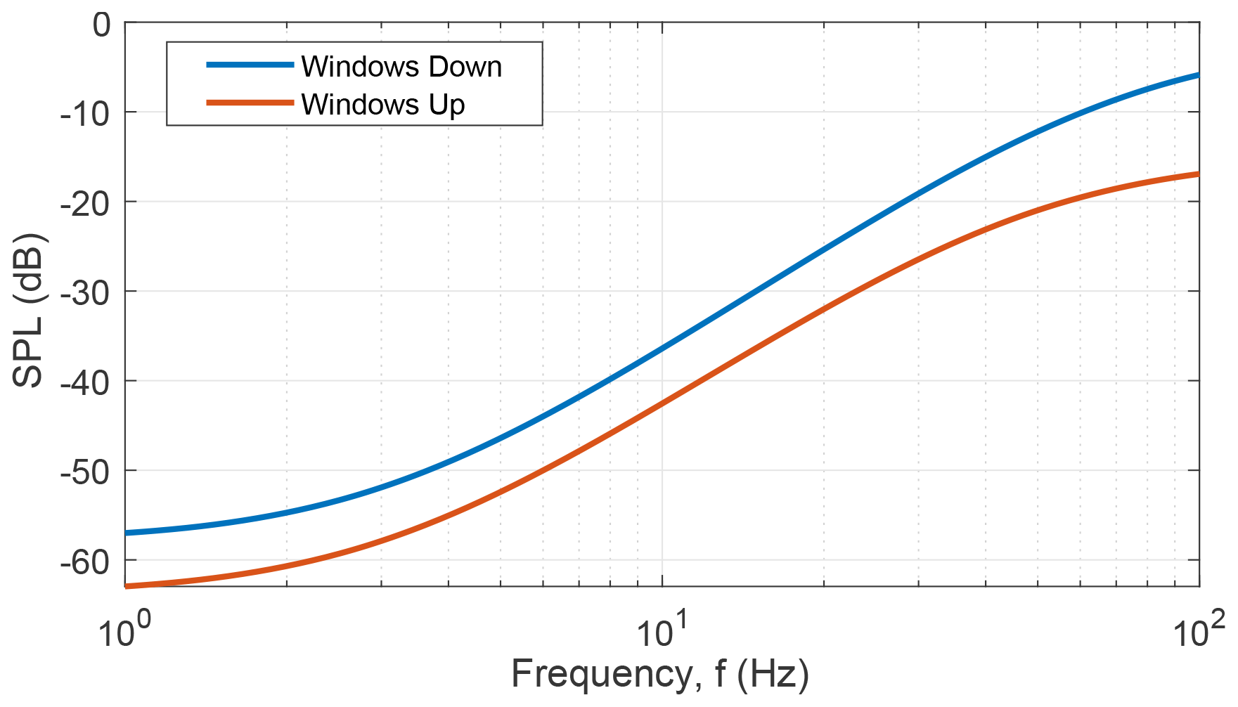
The calibration was conducted in a vehicle example for both windows up and windows down. The window position may have varied during storm-chasing events, and the spectral analysis and peak finding algorithm in Sects. 6.2 and 6.3 are discussed relative to the recorded signal (as implemented in the real-time workflow), and only a single unit is analyzed. For analysis of the underlying physical mechanisms responsible for tornado infrasound or for comparison between multiple units, the truck's acoustic response may be removed by applying the inverse of the calibration transfer function.

6.2 Spectral results

The spectral content recorded on GLINDA before, during, and after the Lakin tornado are compared in Fig. 12. To reduce the effect of the significant spectral slope, a linear regression was computed as SPL change (dB) per frequency decade for pre-event, post-event, and during-event conditions as defined in Eq. (7) and over the frequency range of [0.1, 250] Hz. The trend lines have slopes within 0.5 dB per decade of each other as shown in Fig. 11, while the varied 1 Hz intercepts also suggest an overall rise in spectral energy content across the band of interest during tornado interception. Acoustic work often associates broadband SPL rise below 500 Hz with wind (Nelke et al., 2016, 2014; Lin et al., 2014), which does not necessarily extrapolate to the sub-acoustic region under consideration here.

$$\begin{array}{}\text{(7)}& {\widehat{X}}_{\text{SPL}}\left(f\right)=a_{\mathrm{0}}{\log }_{\mathrm{10}}\left(f\right)+a_{\mathrm{1}}\end{array}$$

Figure 10 Standard deviation of spectra.

Figure 11 Linear fit parameters.

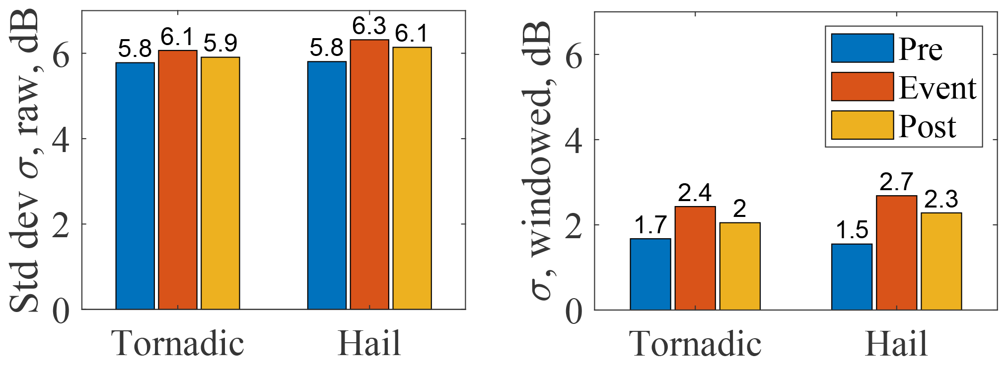
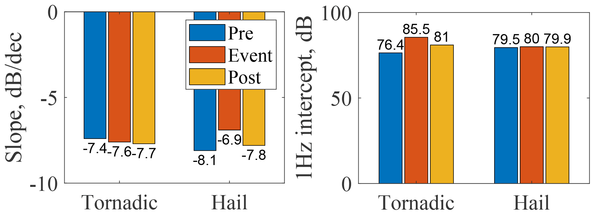
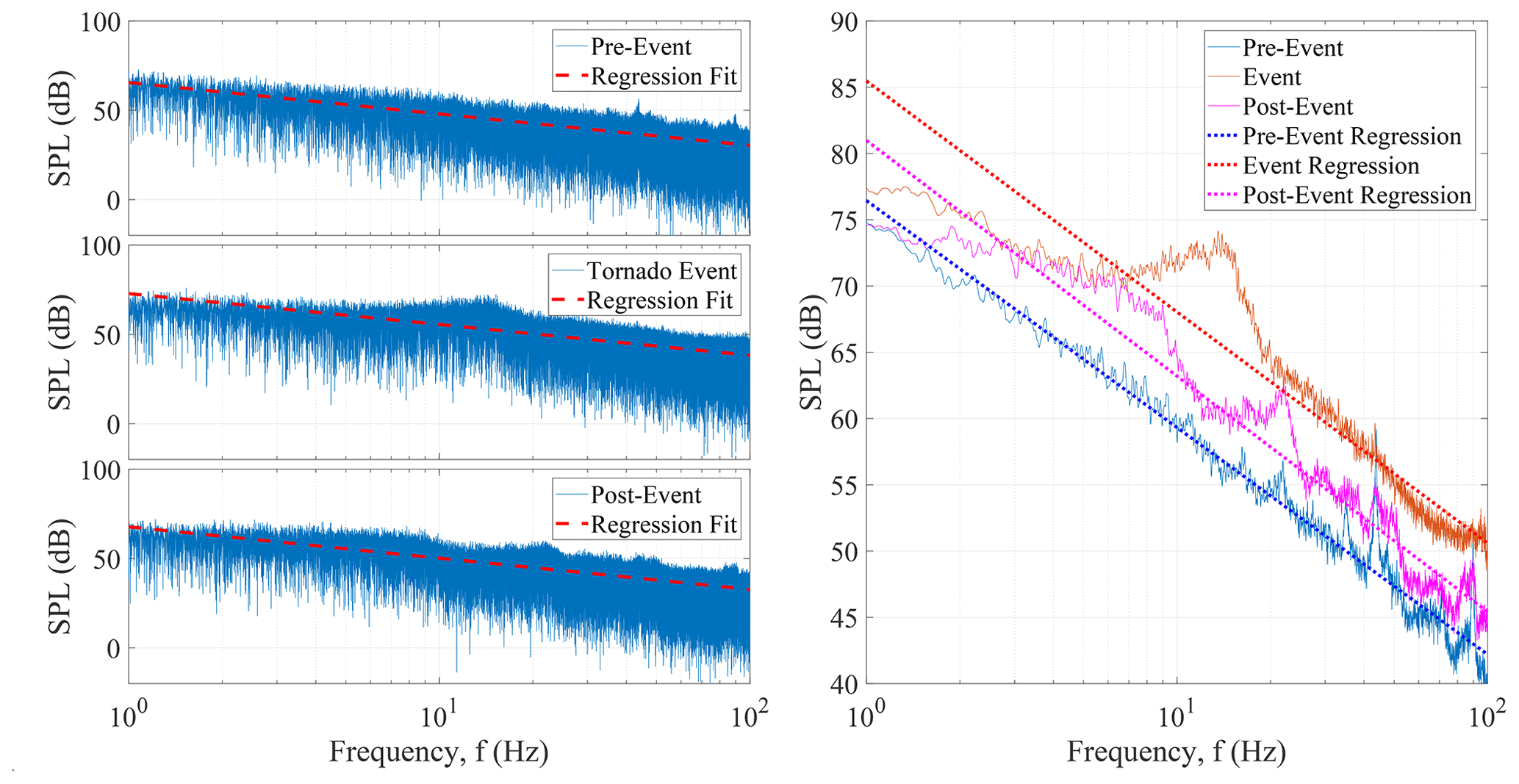
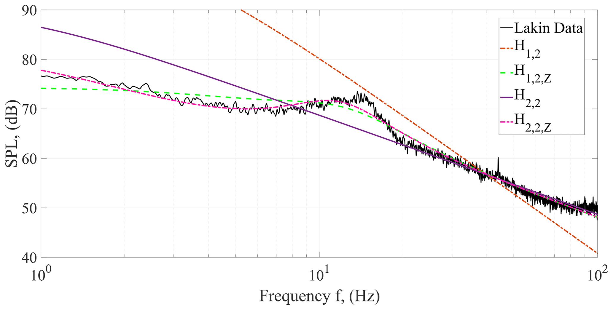
Figure 12 Frequency-domain GLINDA data during the Lakin, KS, tornadic event that occurred from 00:11 to 00:24 UTC on 22 May 2020.

The variance about the best fit curve for each case illustrates the noise reduction in frequency domain due to windowed averaging. The raw and windowed variances for the pre-, post-, and during-tornado intervals are provided in Fig. 10. This comparison shows that the frequency-domain averaging provided by windowing reduced the numerical variance from 33–35 dB in the raw transform to 2.9–5.9 dB variance in the windowed transform. This noise reduction significantly improves the ability to resolve features with changes in the 3–6 dB magnitude range. From this variance reduction, the elevated signal in the 10 to 15 Hz frequency band during the tornado is made more apparent. The center of this frequency band (10–15 Hz) shows a 9 dB rise above the linear fit, and this rise over this frequency band is not present 1 h prior to or 1 h following the tornadic activity.

The 10–15 Hz elevated frequency band during the tornado accounts for 3.3 dB (and therefore the majority) of the variance during the tornadic event, and the peak falling within this range is consistent with this being a relatively small tornado. Tornado infrasound is consistently reported with a fundamental frequency in the 0.5 to 10 Hz range (Bedard, 2005) – with the smaller the tornado, the higher the frequency. Elbing et al. (2019) observed a similar small EFU tornado, and its fundamental frequency was estimated to be 8.3 Hz. These observations are nominally consistent with the analysis of Abdullah (1966) that predicts $f_n=(\mathrm{4}n+\mathrm{5})c/\mathrm{4}d$, where f_n is the frequency of mode n; c is the speed of sound; and d is the diameter of the vortex core. There are fundamental issues with this analysis, but all of the results published in archival journals (Bedard, 2005; Frazier et al., 2014; Dunn et al., 2016; Elbing et al., 2019) nominally follow this trend (though generally aligning better with the first overtone, n=1). Thus it is appropriate to use this relationship as a nominal empirical relationship. This analysis predicts that a tornado with a fundamental frequency of 12.5 Hz would have a vortex core diameter of 34 m. Past observations indicate that this estimate is likely to be low, and the actual tornado core that would produce a 12.5 Hz fundamental frequency would fall in the range of 35–90 m. This is still below the reported maximum damage path width (137 m). However, having a similar magnitude is likely all that can be expected given the uncertainty in the analysis, damage assessment (both estimated values as well as only reporting the maximum), and relationship between vortex core and damage width. Note that the largest tornadoes have core diameters well in excess of 1000 m.

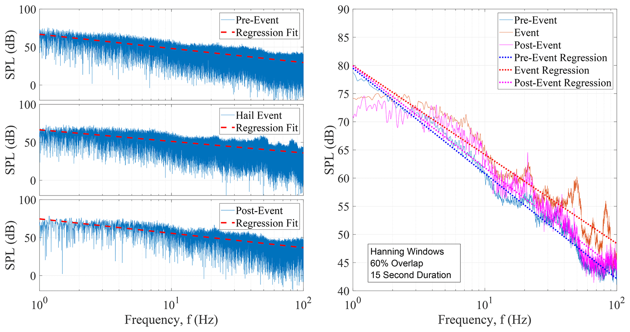
Figure 13 Frequency-domain infrasound measured with GLINDA during the Comanche County hail event at 23:15 UTC on 22 May 2020.

Figure 14 First-stage model fit to Lakin, KS, tornado infrasound/low-sonic measurements.

The spectral content associated with the Commanche County hail event is shown in Fig. 13. As with the Lakin tornado analysis, calculation of best fit lines (defined in Eq. 7 with fitting parameters listed in Fig. 11) show over 30 dB reduction for windowed spectra as listed in Fig. 10. The linear best fit lines for the hail event do not show significant SPL differentials between the three intervals (pre-, post-, and during-event hail) at the lower end of the measurement range < 10 Hz. The slope of the fit during the hail event is 3 dB per decade higher than the pre-events or post-events, which creates a SPL difference of up to 5 dB over the band of interest. Unlike the Lakin EFU tornado, there was no apparent swell in SPL in the 10 to 15 Hz band. However, smaller rises near 50 and 80 Hz for the event spectra are present with a peak of 6 dB relative to the linear best fit. It is unclear what is responsible for these peaks, but these features are at frequencies above what is typically associated with severe weather (though some overtones have produced signals in the audible range). In the frequency range of interest (nominally 1–10 Hz), there is no apparent signal that was produced. This is consistent with past observations that have noted that hail-producing storms without tight rotation typically do not produce an infrasound signal (Petrin and Elbing, 2019).

6.3 Peak identification results

For the tornadic measurements, an infrasound peak was present, and the results of the two-stage model fitting process in Fig. 6 are presented in Tables 3 and 5.

Table 3 Mean-squared error for various first-stage curve fits to raw data.

From the first-stage model fits, a first-order fit has the lowest mean-squared error (MSE) between the tested transfer function models. The first-order model and second-order model were further investigated through a second-stage transfer function model fitting. To develop the second grouping of models, the difference between the raw data and the first-stage models was compared to a more select group of transfer functions based on observable characteristics in the resulting difference signal – namely, the rise over the 10–15 Hz band and the flat region in the audible range. Results of the overall model fits comprised by adding the fitted models from the secondary analysis to the first-stage model fit are presented in Table 4 where values of the percent errors for detected frequency for the peak (Eq. 8) and detected peak magnitude (Eq. 9) were calculated relative to manually gathered values. The MSE for the combined fits is additionally presented.

$$\begin{array}{}\text{(8)}& {\displaystyle }{E}_{f_{\mathrm{p}}}=\mathrm{|}{\displaystyle \frac{f_{\mathrm{p}}-{\widehat{f}}_{\mathrm{p}}}{{\widehat{f}}_{\mathrm{p}}}}\mathrm{|},\text{(9)}& {\displaystyle }{E}_{\mathrm{|}H{\mathrm{|}}_{\mathrm{p}}}=\mathrm{|}{\displaystyle \frac{\mathrm{|}H{\mathrm{|}}_{\mathrm{p}}-{\widehat{Y}}_{\mathrm{p}}}{{\widehat{Y}}_{\mathrm{p}}}}\mathrm{|}.\end{array}$$

Although $H_{\mathrm{2},\mathrm{2},Z}$ has the lowest overall MSE and percent error for peak magnitude, the coefficients returned by the optimization process are of high order and have significantly higher adjacency value bounds as compared to first-stage, first-order fits (Table 5), creating overfitting concerns. $H_{\mathrm{1},\mathrm{2},z}$ by contrast does not produce similarly large coefficients and low adjacent value bounds. This is achieved while only producing a 3 percentage point increase in the peak percent error and 0.8 dB² mean-squared error over the frequency band, suggesting it may be a more viable model candidate. An additional round of fits was completed for the $H_{\mathrm{1},\mathrm{2},Z}$ model structure implementing a log frequency weighting to the mean-squared error formulation in Eq. (4) as a decadal Gaussian distribution centered on f = 10 Hz. The weighting scheme decreased $E_{\mathrm{|}H{\mathrm{|}}_{\mathrm{p}}}$ by 12 % in exchange for f_p and MSE increasing 3 %. Because the focus of this modeling approach is largely concerned with peak frequency identification, the usage of this weighting method was not further implemented for usage.

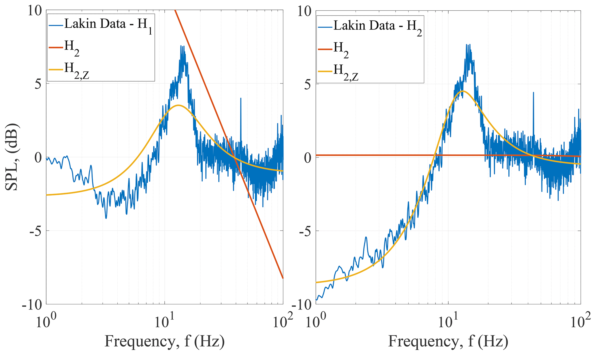
Figure 15 Secondary curve fits to Lakin, KS, tornado measurements with select first-stage fits subtracted.

Table 4 Fit parameters for the four model structures.

Figure 16 Comparison of frequency-domain model fits to Lakin, KS, tornado measurements.

The model structure fitting process is a nonlinear minimization that is prone to local minima or poorly fit terms. To examine the robustness of the model fits to differing initial guesses, a Monte Carlo approach to fitting model uncertainty was implemented by taking 1000 initial parameter guesses uniformly distributed over 1 order of magnitude surrounding what is an expected range of values.

Table 5 Median fit parameters uncertainty distribution as quantified by Monte Carlo convergence over 1000 initial guesses.

7 Conclusions

Sparse tornadic infrasound measurements have limited their application in predictive work. To improve the availability and quality of observations of infrasound from tornadoes, the Ground-based Local INfrasound Data Acquisition (GLINDA) system that includes an infrasound microphone, an IMU, and a GPS receiver has been designed and deployed. The infrasound microphone has a sensitivity of 0.401 V Pa⁻¹ with a flat (to −3 dB) response from 0.1 to 200 Hz, and the 36 V peak-to-peak analog output is sampled at 2050 Hz via ADC to mitigate aliasing of signals with significant magnitude. This microphone, voltage divider circuit, and ADC measurement path maintains a resolution of 1.4 mPa, which sets the quantization error below existing noise floor estimates from existing array measurements at 20 mPa. The GLINDA system operates on a Raspberry Pi 3B+ platform with the data exported to an online repository and processed for real-time display of spectra and model fitting in an online display portal with update rates similar to radar. The processing tools incorporate the chirp Z-transform and windowing to reduce the uncertainty of the signal, as verified by a 50 % reduction in standard deviation.

GLINDA was installed in a storm-chasing vehicle and has been acquiring data from May 2020 to present. It has recorded several severe weather events, including a dust storm, gustnado, fires, and significant hail. This paper provides design details and analysis from two events – a tornado and a significant hail storm. The tornado occurred in the early hours of 22 May 2020 near Lakin, KS. The tornado lasted 13 min, had a length of 2.8 km, and a maximum damage path width of 137 m (and unknown strength). The storm chasers measured this system from 4 km SSE of the tornado. The spectral content shows an elevated signal during the tornado spanning 10 to 15 Hz, consistent with past observations of small tornadoes as described in Sect. 2. The hail event occurred the following evening at 23:15 UTC on 22 May 2020 with 25.4 mm hail while the storm chasers were located in Oklahoma's Comanche County. A similar spectral analysis was performed on this event, but no significant infrasound production was identified relative to periods before and after the hail.

These results indicate consistency of the mobile observations with fixed measurements and support this modality as a means of increasing the availability and signal-to-noise ratio of tornado infrasound observations, and the analysis shows an improvement in precision enabled by real-time model-fitting-based processing tools to resolve and quantify spectral deviations associated with tornado activity.

Appendix A: NWS WSR-88D scanning frequency

Figure A1 WSR-88D MESO-SAILS scanning regiment with average times for measurement sweeps; from NOAA (2014).

Appendix B: Tornado event auxiliary data

B1 Reflectivity measurements

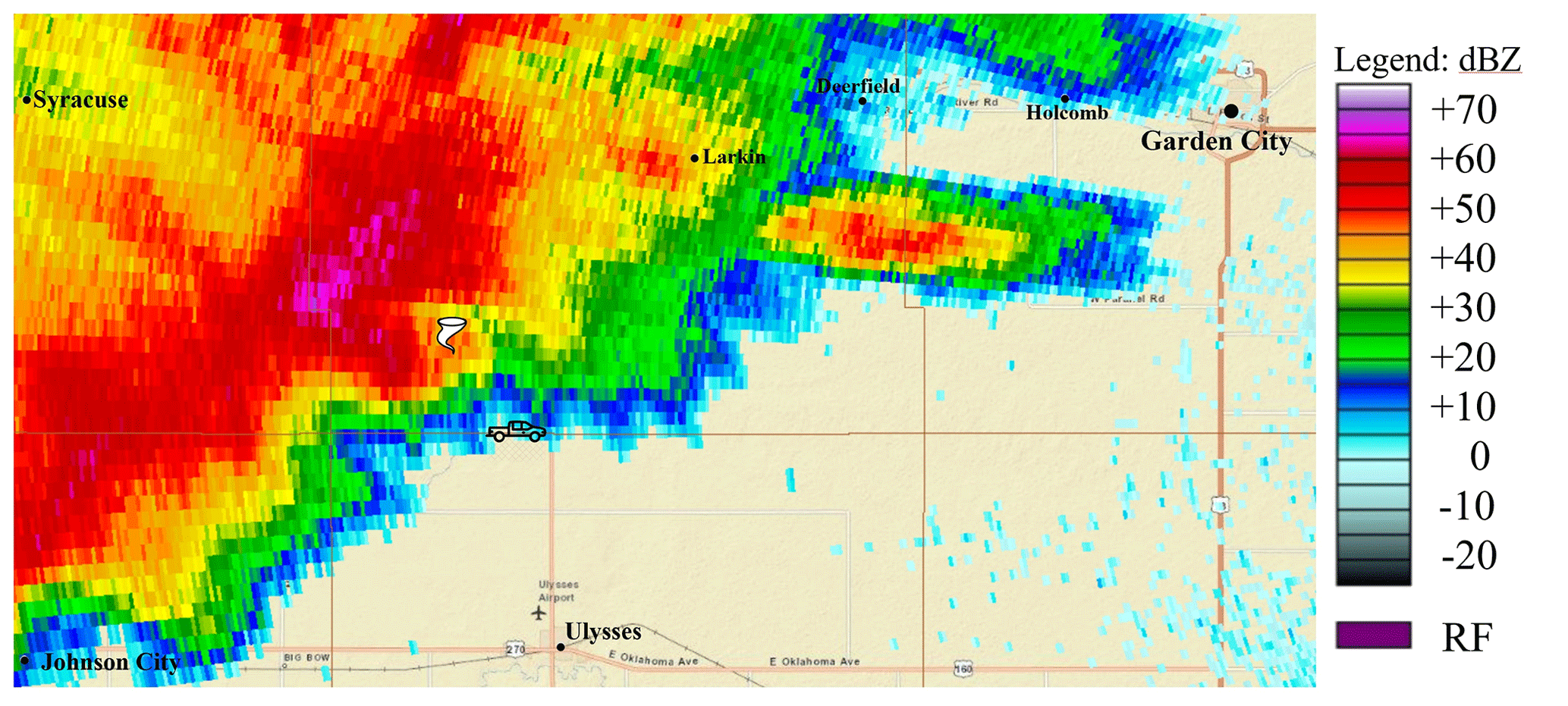
Figure B1 KDDC (Dodge City Regional Airport, KS) reflectivity measurement at 22 May 2020, 00:17 UTC, with elevation of the scan = 2590 ft (790 m) (lowest possible base scan). The tornado location is indicated via the tornado icon and the storm-chaser region of intercept via the truck icon.

B2 Radial velocity measurements

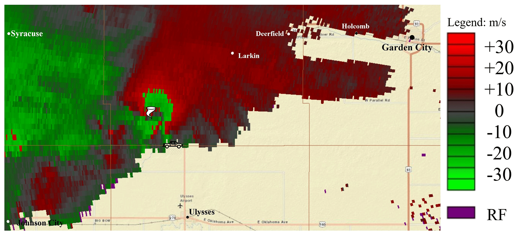
Figure B2 KDDC (Dodge City, KS) radial velocity measurement at 22 May 2020, 00:17 UTC, with elevation of the scan = 2590 ft (790 m) (lowest possible base scan). The tornado location is indicated via the tornado icon and the storm-chaser region of intercept via the truck icon.