Observation error analysis for the WInd VElocity Radar Nephoscope W-band Doppler conically scanning spaceborne radar via end-to-end simulations

The WIVERN (WInd VElocity Radar Nephoscope) mission, now in Phase 0 of the ESA Earth Explorer program, promises to complement Doppler wind lidar by globally observing, for the first time, the vertical profiles of winds in cloudy areas. This work describes an initial assessment of the performances of the WIVERN conically scanning 94 GHz Doppler radar, the only payload of the mission. The analysis is based on an end-to-end simulator characterized by the following novel features tailored to the WIVERN radar: the conically scanning geometry, the inclusion of cross-polarization effects and the simulation of a radiometric mode, the applicability to global cloud model outputs via an orbital model, the incorporation of a mispointing model accounting for thermoelastic distortions, microvibrations, star-tracker uncertainties, etc., and the inclusion of the surface clutter. Some of the simulator capabilities are showcased for a case study involving a full rotational scan of the instrument.

Preliminary findings show that mispointing errors associated with the antenna's azimuthal mispointing are expected to be lower than 0.3 m s⁻¹ (and strongly dependent on the antenna's azimuthal scanning angle), wind shear and non-uniform beam-filling errors have generally negligible biases when full antenna revolutions are considered, non-uniform beam filling causes random errors strongly dependent on the antenna azimuthal scanning angle, but typically lower than 1 m s⁻¹, and cross-talk effects are easily predictable so that areas affected by strong cross-talk noise can be flagged. Overall, the quality of the Doppler velocities appears to strongly depend on several factors, such as the strength of the cloud reflectivity, the antenna-pointing direction relative to the satellite motion, the presence of strong reflectivity and/or wind gradients, and the strength of the surface clutter. The end-to-end simulations suggest that total wind errors meet the mission requirements in a good portion of the clouds detected by the WIVERN radar.

The simulator will be used for studying tradeoffs for the different WIVERN configurations under consideration during Phase 0 (e.g., different antenna sizes, pulse lengths, and antenna patterns). Thanks to its modular structure, the simulator can be easily adapted to different orbits, different scanning geometries, and different frequencies.

1 Introduction

Accurate forecasts save lives and support emergency management and the mitigation of impacts, thus preventing losses from severe weather while creating substantial revenue (Bauer et al., 2015). Windstorms are the largest contributor to economic losses caused by weather-related hazards, resulting in approximately USD 500 billion of global damage over the last decade (https://www.ncdc.noaa.gov/billions/, last access: 12 May 2022). Together with floods, they are the costliest natural hazards in Europe. They account for more than 30 % (60 %) of total (insured) losses (https://publications.jrc.ec.europa.eu/repository/handle/JRC118595?mode=full, last access: 12 May 2022). The Aeolus wind lidar has demonstrated a large impact in reducing forecast errors when assimilated by European Centre for Medium-Range Weather Forecasts(ECMWF; Rennie et al., 2021). In addition to winds, cloud and precipitation measurements remain key for both numerical weather prediction (NWP) applications and for advancing understanding of cloud processes and their role in climate simulations.

The WIVERN (WInd VElocity Radar Nephoscope) concept has been recently proposed within the ESA Earth Explorer 11 call in order to strengthen the wind, cloud, and precipitation observation capability of the Global Observing System. The mission has been selected for Phase 0 studies. It hinges upon a single instrument, i.e., a dual-polarization Doppler W-band scanning cloud radar with a 3 m circular aperture non-deployable main reflector. The WIVERN antenna conically scans around nadir at an off-nadir angle of 38^∘ at 12 rpm (revolutions per minute). This rotation speed implies the use of one horn for transmission and another one for reception. Flying on a 500 km orbit, the instrument provides a swath of 800 km (see Fig. 1).

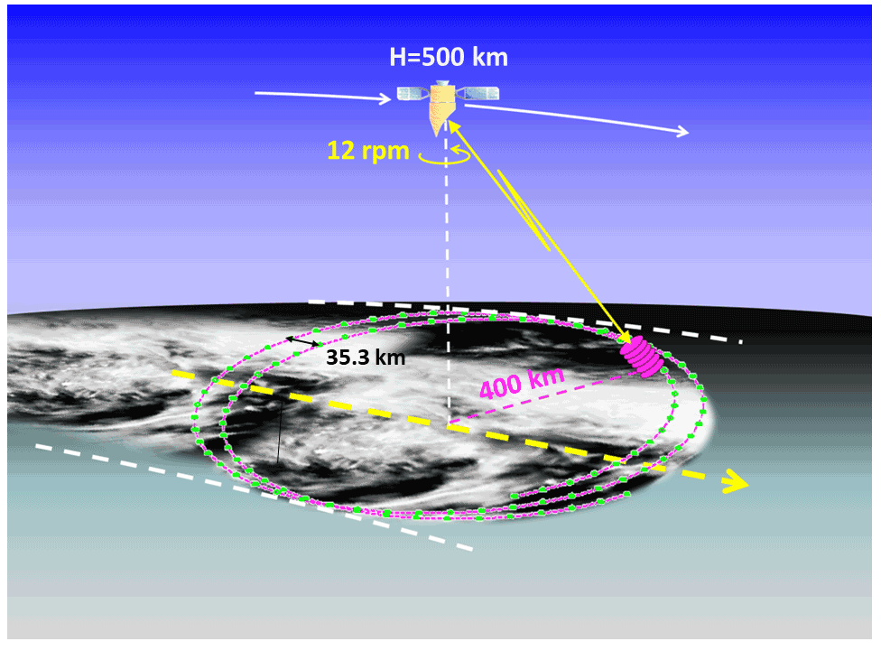
Figure 1 Artistic impression of the WIVERN concept. A 94 GHz Doppler radar with 3 m antenna scanning at 12 rpm tracing out a cycloidal track with an incidence angle of 41.6^∘.

The aim of the mission is to complement Doppler lidar winds acquired in clear-sky conditions and from the tops of optically thick clouds (Rennie et al., 2021) and other wind observations (profiles by radio soundings at cloud top, via geostationary observation-derived atmospheric motion vectors, close to the ocean surface by scatterometers) by observations in areas of optically thick clouds, critical for cyclogenesis, that cannot be seen by optical sensors. Observations in these areas have the largest potential to improve forecasts (McNally, 2002). Therefore, the WIVERN mission is expected to provide the following (Illingworth et al., 2020):

• unprecedented wind observations inside tropical cyclones and mid-latitude windstorms that will routinely reveal the dynamic structure of such destructive systems;

• observations of convective motions that will validate the representation of convection in models;

• global profiles of cloud properties and precipitation over an 800 km swath that will better quantify the hydrological cycle and the atmospheric and surface energy budget; and

• the first direct observation of tropospheric winds that will underpin the predictions of transport and dispersion of trace gases and pollutants in atmospheric chemistry and air quality models.

These advances in the observational capabilities are expected to address the following three science objectives (Illingworth et al., 2020):

1. Extending the lead time of useful prediction skills of hazardous weather (e.g., wind storm, cyclones, and floods) by direct assimilation of wide swath winds from clouds and profiles of radar reflectivity of clouds and precipitation into numerical weather prediction (NWP) models.

2. Improving numerical models by providing new metrics and observational verification to assess different NWP parameterization schemes within such models. NWP and climate models use similar schemes, so better NWP models will also augment confidence in climate models.

3. Establishing a benchmark for the climate record of cloud profiles, global solid/light precipitation, and, for the first time, in-cloud winds, crucial for a better quantification of the Earth's hydrological cycle, and energy budgets, with a significant reduction in the sampling errors of current and planned cloud radar missions.

World Meteorological Organization (WMO) requirements for data assimilation into global NWP (Illingworth et al., 2018) can be found at OSCAR (https://www.wmo-sat.info/oscar/, last access: 12 May 2022) and are summarized in Table 1. The threshold of 12 h for the observing cycle is quite demanding; three scatterometers with 1200 km swaths can approach this revisit time. Noticeably, the Aeolus non-scanning, narrow swath, clear-sky wind measurements are having a significant effect, despite their typical clear-sky uncertainty of 4–5 m s⁻¹ and their coarse sampling (Rennie et al., 2021). Thus, even winds with uncertainty above the WMO threshold and with sampling below threshold have proved to be extremely valuable for NWP. Horanyi et al. (2014) showed that assimilating winds biased by 1–2 m s⁻¹, when the random error is around 2 m s⁻¹, would degrade the forecast, so a bias of less than 1 m s⁻¹ should be added to the specifications of Table 1.

Table 1 WMO (World Meteorological Organization) requirements for horizontal winds for numerical weather prediction (NWP) and the expected performance of WIVERN.

^∗ Global average between ±82^∘ latitude.

In order to achieve these targets, WIVERN will adopt the following:

1. polarization diversity (i.e., the use of successive pulses with independent H and V polarization; Pazmany et al., 1999) in order to overcome both the range–Doppler dilemma and the short decorrelation times produced by the Doppler fading associated with the low Earth orbiting satellite velocity (Battaglia et al., 2013), and

2. a large antenna (3 m) in order to achieve a narrow beam, thus giving a fine vertical resolution and fewer issues related to non-uniform beam-filling (NUBF) biases (Tanelli et al., 2002).

Previous studies (Battaglia et al., 2018), based on the CloudSat climatology of cloud reflectivities, have demonstrated that the WIVERN radar should provide 1–2 million wind observations per day that satisfy the WMO goal of 2 m s⁻¹ precision. However, it is important to define a rigorous framework with which to assess the accuracy and precision of Doppler velocities. For instance, errors introduced by satellite mispointing induced by orbital-dependent thermoelastic distortion of the antenna, by the solar array drive mechanism microvibrations, by the rotating antenna vibration, etc., can seriously affect space-borne Doppler velocity measurements, as previously studied in Doppler scanning radars (Ardhuin et al., 2019) and in Doppler lidars (Weiler et al., 2021). Furthermore, Battaglia et al. (2018) used 2D slant path profiles reconstructed from CloudSat and therefore did not implement the 3D scanning geometry of the WIVERN satellite. A full 3D framework is required to evaluate the importance of non-uniform beam-filling errors and to assess how the quality of the Doppler velocity signal will depend on the antenna scanning viewing angle.

End-to-end (E2E) simulators are paramount tools for evaluating instrument performances in preparatory mission studies. They provide a high-fidelity performance prediction of the overall system. The focus of this study is in the mission performance assessment and error budget computation with a detailed partitioning of the different error contributors. Several radar simulators have been developed in the recent years to simulate space-borne atmospheric radars (e.g., Haynes et al., 2007; Matsui et al., 2013; Dellaripa et al., 2021), including Doppler capabilities (e.g., Kollias et al., 2014; Sy et al., 2014) as envisaged for the EarthCARE W-band Doppler radar (Illingworth et al., 2015). Doppler velocity estimates for that system will be based on the pulse pair technique (Doviak and Zrnić, 2006). The novelty of this work is that our radar simulator is tailored to conically scanning Doppler radars adopting polarization diversity. If selected, the WIVERN radar will be the first radar in space to ever adopt such technology. Therefore, radar simulators have not yet included such novel features. The simulator also incorporates a model accounting for mispointing as potentially caused by different sources like thermoelastic distortions, microvibrations, and star-tracker uncertainties. Finally, it includes an orbital model with the possibility of changing orbit and thus viewing geometry. Section 2 provides a detailed description of all the modules of the E2E simulator, whereas Sect. 3 presents some applications, with examples extracted from a case study and a first assessment of some of the errors related to the Doppler velocity measurements. Conclusions and future work are discussed in Sect. 4.

2 The E2E simulator

Our simulator capitalizes on recent refinements of radar simulators developed within different ESA projects. In particular, it benefits from the inclusion of polarization diversity pulse pair processing and wide swath scanning (Battaglia et al., 2013; Battaglia and Kollias, 2015), the effect of the cross-talk (Wolde et al., 2019) between the H and V channels caused by strongly reflective depolarizing targets (e.g., the melting layer or the surface clutter), and the simulation of passive mode to provide brightness temperatures at W band (Battaglia and Panegrossi, 2020). A simplified 2D version of the simulator has recently been applied to CloudSat observations and co-located ECMWF 3D winds to provide an initial assessment of errors introduced by different sources related to aliasing, averaging, and to the noise in the estimators of the Doppler spectra moments (Battaglia et al., 2018).

The simulator developed in this work can cope with data produced by state-of-the-art, high-resolution cloud-resolving models as the basis for creating scenes that are used as input to the various instrument simulation modules. These outputs can be linked with sun-synchronous orbits produced by an orbital model derived from the two-body problem theory, with the addition of J₂ orbital perturbations. The user can modify the initial date and duration of orbital propagation and the orbital parameters. This provides us with the ability to simulate the satellite overpasses and the measurements for the given viewing geometry. In this control environment, forward and retrieval models can be evaluated and compared against the truth of the input model scene. Similarly, each error source can be evaluated separately, based on the assumption that, as a first approximation, the different error sources can be assumed to be independent, so that the total quadratic error (bias) can be computed as a quadratic sum (an absolute sum) of the different errors (Battaglia and Kollias, 2015). For instance, the satellite motion NUBF-induced errors can be estimated by computing the velocities running the simulator with or without satellite motion and then taking the differences between the two (Battaglia et al., 2018).

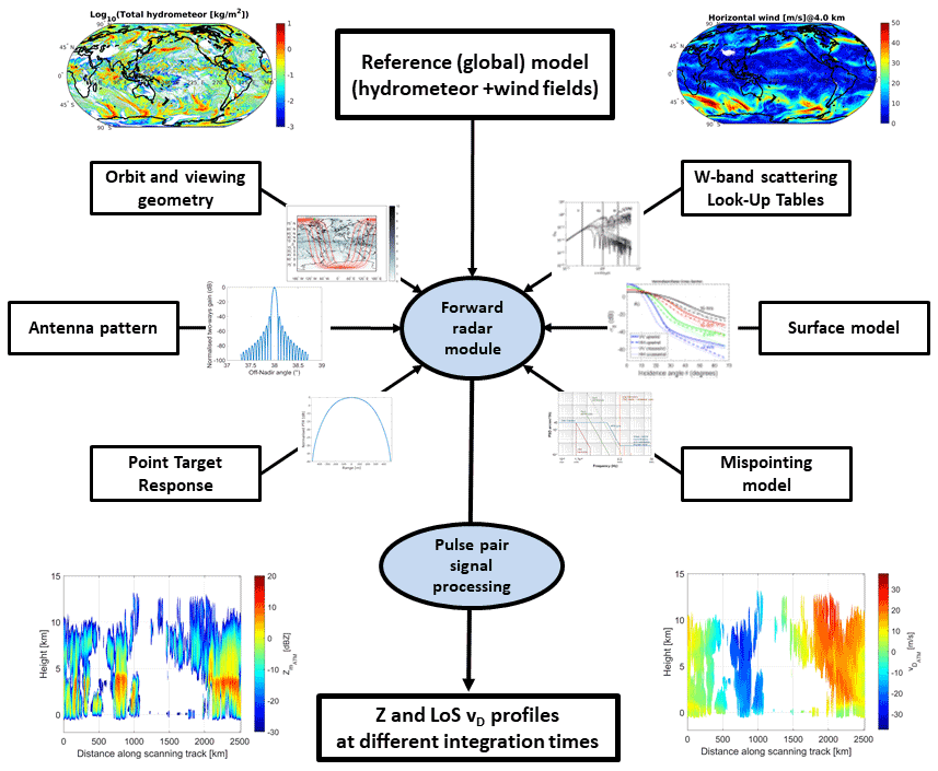
Figure 2 Flow chart illustrating the overall structure of the Wivern E2E simulator. The integrated hydrometeor content and the 4.0 km height winds are shown at the top as examples of input fields from the reference global model whereas outputs of the simulator (reflectivities and line-of-sight (LOS) winds) for a WIVERN cross section that will be examined later (Figs. 12–15) are presented in the bottom colored panels.

Hogan and Battaglia (2008)

Table 2 Current and future capabilities of the WIVERN E2E simulator.

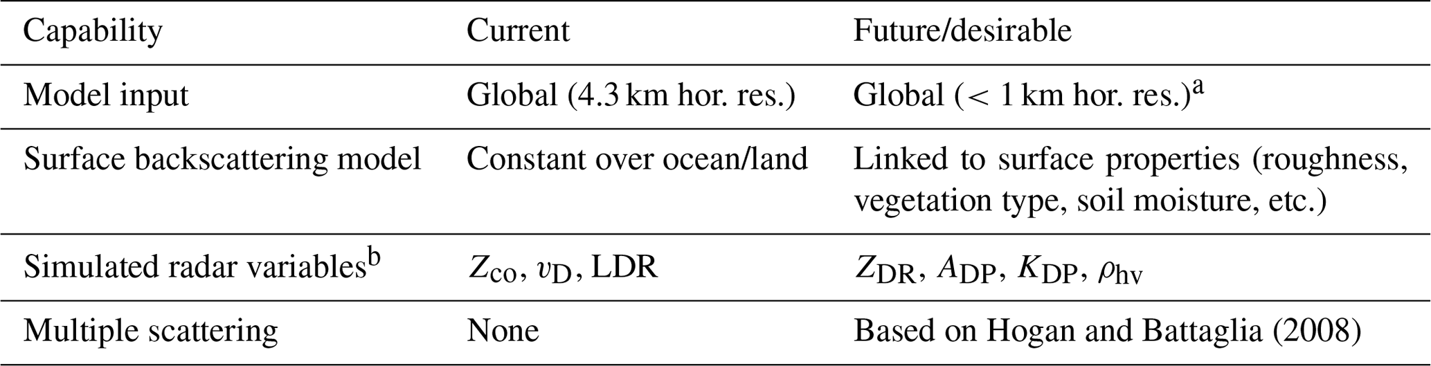
^a Currently, such models are not available and represent a challenge for memory and/or computation time requirements. ^b The meaning of these variables is discussed in the text. Note: hor. res. is the horizontal resolution, and LDR is the linear depolarization ratio.

A schematic for the overall structure of the simulator is depicted in Fig. 2, with a list of current and potential additional capabilities tabulated in Table 2. A global model provides high-resolution 3D scenes with clouds and winds. Outputs of the global model are used as inputs of a forward model that computes ideal profiles of W-band co- and cross-polar reflectivities and Doppler velocities. Note that the forward model is based on the single scattering assumption. Multiple scattering effects are known to play an important role both for the reflectivity and the Doppler velocity signal in deep convective regions in the presence of high attenuation (Battaglia et al., 2010b; Battaglia and Tanelli, 2011). The forward model outputs are then combined in a pulse pair signal processing module, which adds the proper noise levels to produce WIVERN outputs (H and V channel reflectivities and line-of-sight Doppler velocities). Our tool simulates mean quantities and their errors as computed from well-established radar theory (Doviak and Zrnić, 2006) for the specific polarization diversity pulse pair processing (Pazmany et al., 1999). These estimates have been validated by an airborne field campaign (Wolde et al., 2019). Other simulators that compute I and Q time series (Battaglia et al., 2013; Kollias et al., 2014) are avoided here because of their high computational time.

The description of the different modules of the simulator is detailed in the following subsections. The radar specifics used throughout this paper are the ones recently proposed to the ESA Earth Explorer 11 and are listed in Table 3.

Table 3 Specifics of the radar for the simulation. The configuration adopted here is the one proposed for WIVERN in a recent ESA Earth Explorer 11 call. The E2E simulator can study various tradeoffs to optimize mission, system, and instrument parameters.

^∗ A value of −15 dBZ may be assumed to allow for a 3 dB margin.

2.1 The System for Atmospheric Modeling (SAM) global storm resolving model

The global storm-resolving models (GSRMs; Stevens et al., 2019; Satoh et al., 2019) are a new class of high-resolution global numerical models that explicitly simulate small scales of motions coupled to large-scale circulation systems. This allows GSRMs to explicitly resolve deep convection and thus overcome challenges arising from deep convection parameterizations (Kendon et al., 2017). The first intercomparison of GSRMs was conducted in the context of the DYAMOND (the DYnamics of the Atmospheric general circulation On Non-hydrostatic Domains) project (Stevens et al., 2019).

Here, output from a GSRM that participated in the DYAMOND project, the System for Atmospheric Modeling (SAM; Khairoutdinov and Randall, 2003), which employs an anelastic form of the non-hydrostatic equations was used as input to the WIVERN radar simulator. The SAM has a horizontal resolution of 4.3 km and 74 vertical layers. Details of the SAM model configuration can be found in Stevens et al. (2019). The model output is available at the DYAMOND project website at https://www.esiwace.eu/services/dyamond (last access: 12 May 2022). The model outputs needed are temperature, pressure, and relative humidity profiles, plus the different hydrometeor water-equivalent contents. The different species are assumed to have different gamma size distributions (Testud et al., 2001). In principle, any geolocated model that can produce such outputs can be ingested by the simulator.

2.2 Forward radar module

2.2.1 Orbital model and scanning geometry

The orbit selected for WIVERN is sun-synchronous, with a mean inclination of 97.4^∘, a mean eccentricity of 0.001257, a mean local time of the ascending node equal 06:00 LT and $\mathrm{15}+\mathrm{1}/\mathrm{5}$ orbits per day, which provides global coverage up to ±82^∘ latitudes. An example of the simulation of five orbits is shown in Fig. 3. By running several orbits, it is possible to compute, for each location, the mean and maximum (i.e., the worst-case scenario) revisit time of the WIVERN radar footprint; the latter is plotted as a function of latitude and longitude in Fig. 4a. The maximum revisit time has a strong latitudinal behavior with a minimum in the equatorial band (peaking at more than 5 d) and a secondary peak at $\sim \pm \mathrm{46}$^∘ (exceeding 3 d at some longitudes). The maximum (blue line) and mean (red line) revisit time averaged over all longitudes as a function of latitude are shown in Fig. 4b. While the maximum revisit time presents different local maxima, the mean revisit time is monotonically decreasing from the Equator to the poles, with a mean value of 1.5 d in the tropical band and of less than 1 d above 50^∘ latitude, which leads to an average global revisit time of once a day between ±82^∘ latitude.

Figure 3 Example of a simulation of five WIVERN orbits with the ground tracks (red lines) and the 800 km WIVERN scanning swath (red-shaded region) plotted over the hydrometeor one-way path integrated W-band attenuation (the color bar scale is in dB). A single model snapshot is used for the simulation.

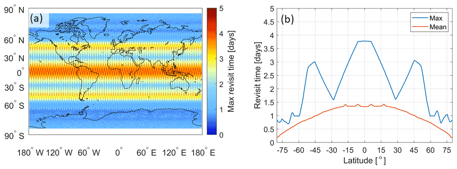
Figure 4 (a) WIVERN maximum (i.e., the worst-case scenario) revisit time for a $\mathrm{15}+\mathrm{1}/\mathrm{5}$ d orbit. (b) The red dotted and blue continuous lines correspond to the latitude-averaged mean and maximum revisit time, respectively, as a function of latitude. Note a mean revisit time of 1.5 d in the tropical band and of less than 1 d above 50^∘ latitude. Globally, the mean revisit time is roughly daily.

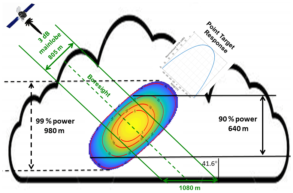
The radar is sounding the atmosphere down to the ground with a range resolution of 500 m. Figures 5 and 6 illustrate the observing slant geometry. The actual vertical resolution will be the result of the slant range resolution, the antenna beamwidth, and the satellite altitude (Meneghini and Kozu, 1990). Note that, for a uniform cloud, 90 % (99 %) of the backscattering power is coming from a region whose vertical extent is 640 m (980 m). The horizontal sampling pattern is a function of the rotation speed. The values used here (Table 3) are the result of a preliminary optimization for wind product performance (sensitivity and spatial resolution).

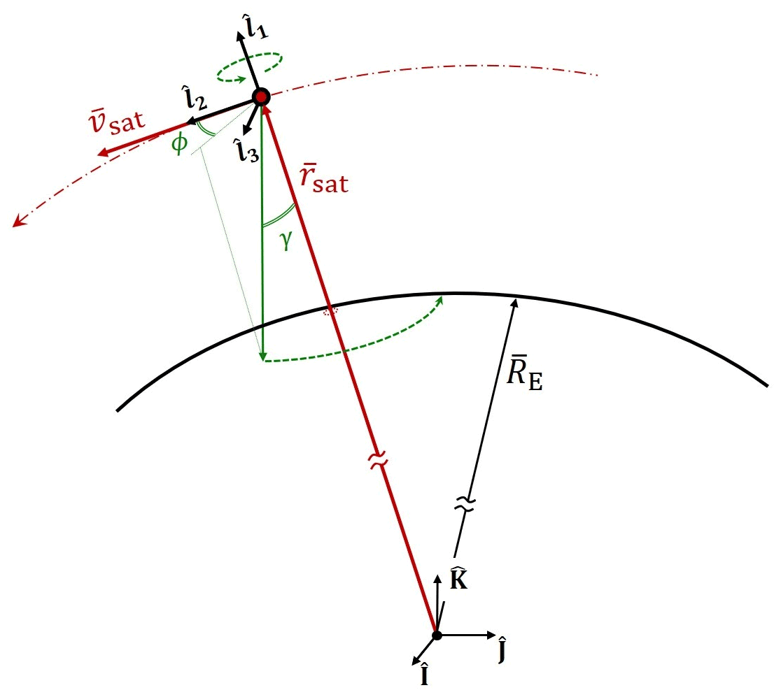
Figure 5 Illustration of the satellite-scanning geometry. The boresight direction (solid green arrow) is identified by the elevation angle γ=38^∘ with respect to the nadir direction and by the azimuth angle ϕ measured from the horizontal direction ${\widehat{l}}_{\mathrm{2}}$ of the local–vertical/local–horizontal (LVLH) reference frame. The solid red arrows r_sat and v_sat represent the satellite's position and velocity vectors in the geocentric–equatorial (IJK) reference frame.

Figure 6 Schematic illustrating the 2D projection onto the antenna elevation cut of the WIVERN observing geometry. The specifics of the radar are detailed in Table 3.

2.2.2 W-band scattering look-up tables

Scattering properties (extinction and backscattering coefficients, single scattering albedo, asymmetry parameters, and Doppler velocities) at each model grid point are computed by adding up the contributions from the different hydrometeors (cloud water, cloud ice, rain, and snow). Gas attenuation is computed according to the Rosenkranz (1998) model. The total scattering, backscattering, and extinction coefficients are derived by adding up the single particle scattering, backscattering, and extinction cross sections for the different hydrometeor species according to their particle size distributions. Since all particle size distributions in the model are gamma size distributions, scattering properties are tabulated per unit mass concentration as a function of the mean mass weighted diameter and of the μ parameter (and of temperature, in case of liquid hydrometeors) like in the appendix of Battaglia et al. (2020b). Mie theory (Lhermitte, 1990) is used to compute the single particle scattering properties. The class “snow” (which represents all large ice particles) is assumed to have a constant density of 0.1 g cm⁻³, with the refractive index computed according to Maxwell–Garnett mixing formula (Kneifel et al., 2020). An exponential drop size distribution (μ=0) is assumed both for rain and snow, with $N_{\mathrm{0}}=\mathrm{8}\times {\mathrm{10}}^{\mathrm{6}}$ m⁻⁴ (Marshall and Palmer, 1948) and N₀=10⁸ m⁻⁴, respectively. The single scattering albedo is just the ratio between the scattering and the extinction coefficients, whereas the asymmetry parameter is derived as a weighted average of the different species asymmetry parameters with the scattering coefficients as weights. Currently, the simulator only accommodates ice particles with fixed ice densities and hydrometeors with spherical shapes. The first issue can be resolved by changing the assumptions and switching the reference scattering look-up table. On the other hand, the inclusion of preferentially oriented hydrometeors and dichroic media, which requires a polarization-dependent treatment of scattering and extinction (Battaglia et al., 2010a), is more complex. Such depolarization effects are not deemed to be as large at W band as at lower frequencies, but they may be important by producing measurable differential phase shifts in ice clouds (Myagkov et al., 2020) and in deteriorating the Doppler velocity estimates by introducing decorrelation between the closely separated H- and V-polarized pulses adopted with polarization diversity (Wolde et al., 2019). The inclusion of polarimetric variables is planned as future development (see Table 2) and will allow us to compute parameters (Bringi and Chandrasekar, 2001) like differential attenuation, A_DP, reflectivity differential ratio, Z_DR, cross-correlation coefficient, ρ_hv, and phase differential shift, K_DP. In order to simulate the cross-polar reflectivities, linear depolarization ratio (LDR) values are assigned to the different hydrometeor species based on LDR climatology collected at the Chilbolton observatory (see Battaglia et al., 2018). The different hydrometeors of the model output are assigned LDR values drawn from a normal distribution with 1.5 dB standard deviation and mean values of −21, −19, −19, and −30 dB for rain, ice crystals, snow, and cloud, respectively. LDRs in the assumed melting layer (at temperatures between the −1 and +4 ^∘C isotherm) are assumed to have a mean value of −14 dB and a standard deviation of 1.5 dB. Note that the 5 ^∘C range of temperature allowed for the melting layer generally tends to overestimate the thickness of the melting layer; thus, the impact of the melting layer induced cross-talk can be overestimated. The LDR values are only relevant when considering the cross-talk effects; at this stage, we believe this approach is sufficient for demonstrating what the climatological impact of the ghosts is in worsening Doppler velocity precisions (Sect. 2.3.2).

2.2.3 Surface model

The normalized surface backscattering cross sections (σ₀; Meneghini and Kozu, 1990) are assumed to be normally distributed around −25 and −8 dB for sea and land, respectively, with 3 dB standard deviation, whereas the surface LDR is assumed to be −14 and −6 dB for sea and land, with 1 dB standard deviation (Battaglia et al., 2017). In the case of coastal regions, a weighted mean accounting for the surface type fraction is taken.

2.2.4 Point target response

The point target response (PTR) is assumed to be a simple top hat with a pulse length, τ_p, of 3.3 µs. Correspondingly, the range resolution becomes $\mathrm{\Delta }r=c{\mathit{\tau }}_{\mathrm{p}}/\mathrm{2}$. A more sophisticated PTR function could be used in order to optimize the equivalent noise bandwidth and PTR width (Fig. 7a). The PTR is used as a convolution function along a range for all the radar observables.

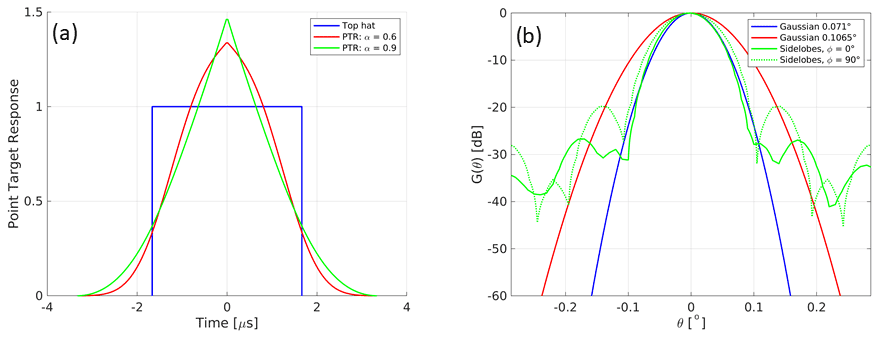
Figure 7 (a) Examples of point target responses that can be used as inputs in the simulator. The narrow top hat (blue curve) is the one adopted for the simulations. (b) Examples of antenna patterns that can be used as inputs in the simulator. The narrow Gaussian one (blue curve) is the one adopted for the simulations. The green ones correspond to the elevation and azimuthal cut of an antenna pattern for an elliptical antenna with sidelobes.

2.2.5 Antenna pattern

Since the WIVERN antenna is circular, a simple Gaussian antenna pattern is assumed with a one-way gain equal to the following:

$$\begin{array}{}\text{(1)}& G\left({\mathit{\theta }}_{\mathrm{a}}\right)=G_{\mathrm{0}}\exp \left[-\mathrm{4}\log \left(\mathrm{2}\right){\left({\displaystyle \frac{{\mathit{\theta }}_{\mathrm{a}}}{{\mathit{\theta }}_{\mathrm{3}\mathrm{dB}}}}\right)}^{\mathrm{2}}\right]\equiv G_{\mathrm{0}}{f}_{\mathrm{a}}\left({\mathit{\theta }}_{\mathrm{a}}\right),\end{array}$$

where G₀ is the antenna gain in the boresight direction, θ_a is the antenna polar angle with respect to the boresight, and θ_3 dB is the antenna 3 dB beamwidth. Any antenna pattern inclusive of side lobes can be added by simply sampling it on the angles used later on for the solid angle integration (Fig. 7b).

2.3 Simulation of polarization diversity radar observables

The Doppler velocity in radar systems is derived by measuring phase shifts between successive pulses (pairs). Since phases are measured with a 2π periodicity, this methodology introduces an ambiguity with a folding Nyquist velocity equal to $v_{Ny}=\pm \frac{\mathit{\lambda }}{\mathrm{4}\mathrm{PRI}}$. This issue could be mitigated by reducing the pair repetition interval (PRI). However, this has the drawback of decreasing the maximum unambiguous range ($r_{max}=c\mathrm{PRI}/\mathrm{2}$) and, in space-borne applications, can actually significantly reduce the correlation between pulses (thus undermining the Doppler methodology). In order to solve this range/correlation–Doppler dilemma, the pulse scheme illustrated in Fig. 8 has been proposed (Pazmany et al., 1999; Kobayashi et al., 2002; Battaglia et al., 2013). Horizontally and vertically polarized pulses are sent out with a short time separation (indicated as T_hv in the diagram) with relatively low repetition frequency; this effectively decouples the maximum unambiguous range from the Nyquist velocity because the H and V pulses propagate, backscatter, and can be received almost independently.

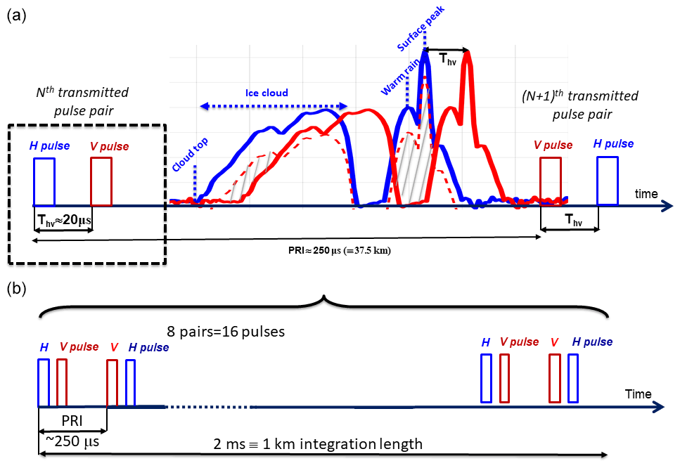
Figure 8 (b) The timing of the transmitted pulse sequence proposed for WIVERN with interlaced H-V pairs. A sequence of M=8 pairs correspond to 2 ms, equivalent to a 1 km distance along the scanning track. Note that the order of the polarization state of each pulse pair is switched from pulse to pulse in order to cancel out differential phase shift effects between the two channels. (a) Example of the return echoes from a scene including an ice cloud, a cloud-free region, and warm rain above a strongly reflecting surface. The returns in the H channel are plotted in blue and those in the V channel (lagging by 20 µs) in red. The dashed red line corresponds to the interference caused by the blue H pulse encountering a depolarizing target. A very high depolarization ratio of −10 dB has been used to exacerbate this effect that leads to returns in regions void of hydrometeors (later referred to as ghosts) in the red H channel. The hatched areas represent ranges where the ghosts exceed the co-polar signal. In this case, the one from the ground and the warm rain is much more serious (and appears shifted upward by circa 3 km in correspondence to the cloud-free region) than the one caused by the large Z gradients at the top of the cloud. A similar reasoning applies to the H channel (not shown for clarity of purpose).

WIVERN will transmit pairs of 3.3 µs long H- and V-polarized pulses with a separation of T_hv=20 µs at a pulse repetition frequency of 4 kHz (Fig. 8). This parameter selection corresponds to $v_{Ny}=\pm \mathrm{37.5}$ m s⁻¹, sufficiently high for unfolding the highest winds, and to $r_{max}=\mathrm{37.5}$ km.

The fundamental radar quantities are the range dependent I and Q time series. The simulation of I and Qs for a system adopting polarization diversity is described in Battaglia and Kollias (2015). Here we are interested in the level 1 radar observables of reflectivities and Doppler velocities. Thus, we adopt a simpler approach and use theoretical results to derive the noisiness of the reflectivity and velocity fields. Both the volume scattering from the atmosphere and the surface scattering from the ground return must be accounted for when computing such observables.

2.3.1 Simulation of reflectivities

The power received by the radar from the atmosphere, $P_{\mathrm{r}}^{\mathrm{atm}}\left(t\right)$, is given by an integral over the backscattering volume as follows (Bringi and Chandrasekar, 2001):

$$\begin{array}{}\text{(2)}& \begin{array}{rl}{P}_{\mathrm{rec}}^{\mathrm{atm}}\left(t\right)& =P_{\mathrm{tr}}{\displaystyle \frac{G_{\mathrm{0}}^{\mathrm{2}}{\mathit{\lambda }}^{\mathrm{2}}}{(\mathrm{4}\mathit{\pi }{)}^{\mathrm{3}}}}\underset{{\mathit{\varphi }}_{\mathrm{a}}=\mathrm{0}}{\overset{\mathrm{2}\mathit{\pi }}{\int }}\underset{{\mathit{\theta }}_{\mathrm{a}}=\mathrm{0}}{\overset{\mathit{\pi }}{\int }}{f}_{\mathrm{a}}^{\mathrm{2}}\left({\mathit{\theta }}_{\mathrm{a}}\right)\\ & \times \underset{\mathrm{0}}{\overset{\mathrm{\infty }}{\int }}{\displaystyle \frac{\mathit{\eta }(r,{\mathit{\theta }}_{\mathrm{a}},{\mathit{\varphi }}_{\mathrm{a}})}{r^{\mathrm{2}}}}{\left|\mathrm{PTR}(t-\mathrm{2}r/c)\right|}^{\mathrm{2}}\\ & \times e^{-\mathrm{2}{\int }_{\mathrm{0}}^r{k}_{\mathrm{ext}}\left(s\right)\mathrm{d}s}\mathrm{d}r\mathrm{d}{\mathrm{\Omega }}_{\mathrm{a}},\end{array}\end{array}$$

where η is the radar reflectivity or backscattering cross section per unit volume, P_tr is the transmitted power, λ is the wavelength of radar, k_ext is the extinction coefficient, ϕ_a is the azimuthal angle in the antenna reference system, and dΩ_a=sin θ_a dθ_a dϕ_a is the infinitesimal antenna solid angle. The equivalent radar reflectivity factor, Z, is the quantity that is generally used in meteorology instead of η. It is defined as follows:

$$\begin{array}{}\text{(3)}& Z={\displaystyle \frac{{\mathit{\lambda }}^{\mathrm{4}}}{{\mathit{\pi }}^{\mathrm{5}}|K_{\mathrm{w}}{|}^{\mathrm{2}}}}\mathit{\eta },\end{array}$$

where $|K_{\mathrm{w}}{|}^{\mathrm{2}}$ is the dielectric factor for water (Bringi and Chandrasekar, 2001). In the following, we assume the convention to set $|K_{\mathrm{w}}{|}^{\mathrm{2}}=\mathrm{0.93}$. Practically, in order to compute the reflectivity factor corresponding to the atmosphere, the three dimensional integral in Eq. (2) is first broken into an integral over the solid angle (defined with respect to the boresight direction); this allows us to compute Z for ranges r_i sampled at distance δr (=100 m, in our case, but adjustable to the specific need) as follows:

$$\begin{array}{}\text{(4)}& \begin{array}{rl}{Z}_{\mathit{\delta }r}^{\mathrm{atm}}\left(r\right)& ={\displaystyle \frac{{\int }_{{\mathit{\varphi }}_{\mathrm{a}}=\mathrm{0}}^{\mathrm{2}\mathit{\pi }}{\int }_{{\mathit{\theta }}_{\mathrm{a}}=\mathrm{0}}^{\mathit{\pi }}{f}_{\mathrm{a}}^{\mathrm{2}}\left({\mathit{\theta }}_{\mathrm{a}}\right)Z_e(r,{\mathit{\theta }}_{\mathrm{a}},{\mathit{\varphi }}_{\mathrm{a}})e^{-\mathrm{2}{\int }_{\mathrm{0}}^r{k}_{\mathrm{ext}}\left(s\right)\mathrm{d}s}\mathrm{d}{\mathrm{\Omega }}_{\mathrm{a}}}{{\int }_{{\mathit{\varphi }}_{\mathrm{a}}=\mathrm{0}}^{\mathrm{2}\mathit{\pi }}{\int }_{{\mathit{\theta }}_{\mathrm{a}}=\mathrm{0}}^{\mathit{\pi }}{f}_{\mathrm{a}}^{\mathrm{2}}\left({\mathit{\theta }}_{\mathrm{a}}\right)\mathrm{d}{\mathrm{\Omega }}_{\mathrm{a}}}}\\ & \equiv {\displaystyle \frac{{\int }_{{\mathit{\varphi }}_{\mathrm{a}}=\mathrm{0}}^{\mathrm{2}\mathit{\pi }}{\int }_{{\mathit{\theta }}_{\mathrm{a}}=\mathrm{0}}^{\mathit{\pi }}{f}_{\mathrm{a}}^{\mathrm{2}}\left({\mathit{\theta }}_{\mathrm{a}}\right)Z_e(r,{\mathit{\theta }}_{\mathrm{a}},{\mathit{\varphi }}_{\mathrm{a}})e^{-\mathrm{2}{\int }_{\mathrm{0}}^r{k}_{\mathrm{ext}}\left(s\right)\mathrm{d}s}\mathrm{d}{\mathrm{\Omega }}_{\mathrm{a}}}{{\mathrm{\Omega }}_{\mathrm{2}\mathrm{A}}}},\end{array}\end{array}$$

where Ω_2A is the two-way antenna main lobe solid angle (equal to $\mathit{\pi }{\mathit{\theta }}_{\mathrm{3}\mathrm{dB}}^{\mathrm{2}}/\left(\mathrm{8}\ln \mathrm{2}\right)$ for a Gaussian antenna). The solid angle integral is performed by sampling 7 polar and 21 azimuthal angles with respect to the antenna boresight by trapezoidal integration. Then, $Z_{\mathit{\delta }r}^{\mathrm{atm}}\left(r\right)$ is convolved with the point target response as follows:

$$\begin{array}{}\text{(5)}& Z^{\mathrm{atm}}\left(r\right)=w_{\mathrm{PTR}}\times Z_{\mathit{\delta }r}^{\mathrm{atm}}\left(r\right),\end{array}$$

where w_PTR is the normalized point target response.

The power received by the radar from the surface at a range r, $P_{\mathrm{r}}^{\mathrm{surf}}\left(r\right)$, is computed by an integration performed over the surface, Σ, which is obtained from the intersection between the surface and the spherical shell with radius between $r-\mathrm{\Delta }r/\mathrm{2}$ and $r+\mathrm{\Delta }r/\mathrm{2}$, with $\mathrm{\Delta }r=c{\mathit{\tau }}_{\mathrm{p}}/\mathrm{2}$ as follows (Meneghini and Kozu, 1990):

$$\begin{array}{}\text{(6)}& \begin{array}{rl}{P}_{\mathrm{rec}}^{\mathrm{surf}}\left(r\right)& =P_{\mathrm{tr}}{\displaystyle \frac{G_{\mathrm{0}}^{\mathrm{2}}{\mathit{\lambda }}^{\mathrm{2}}}{(\mathrm{4}\mathit{\pi }{)}^{\mathrm{3}}}}\underset{\mathrm{\Sigma }}{\int }{\displaystyle \frac{{\mathit{\sigma }}_{\mathrm{0}}({\mathit{\theta }}_{\mathrm{a}},{\mathit{\varphi }}_{\mathrm{a}})f_{\mathrm{a}}^{\mathrm{2}}\left({\mathit{\theta }}_{\mathrm{a}}\right)e^{-\mathrm{2}{\int }_{\mathrm{0}}^r{k}_{\mathrm{ext}}\left(s\right)\mathrm{d}s}}{r^{\mathrm{4}}}}\mathrm{d}\mathrm{\Sigma }\\ & \equiv P_{\mathrm{tr}}{\displaystyle \frac{G_{\mathrm{0}}^{\mathrm{2}}{\mathit{\lambda }}^{\mathrm{2}}}{(\mathrm{4}\mathit{\pi }{)}^{\mathrm{3}}}}{\mathcal{I}}_{\mathrm{surf}}\left(r\right),\end{array}\end{array}$$

where σ₀ is the normalized radar cross section (NRCS). The surface contribution can be written as an equivalent reflectivity term as follows:

$$\begin{array}{}\text{(7)}& Z^{\mathrm{surf}}\left(r\right)={\displaystyle \frac{{\mathit{\lambda }}^{\mathrm{4}}}{{\mathit{\pi }}^{\mathrm{5}}|K{|}^{\mathrm{2}}}}{\displaystyle \frac{\mathrm{1}}{{\mathrm{\Omega }}_{\mathrm{2}\mathrm{A}}}}{\displaystyle \frac{r^{\mathrm{2}}}{\mathrm{\Delta }r}}{\mathcal{I}}_{\mathrm{surf}}\left(r\right).\end{array}$$

The integral ℐ_surf, defined in Eq. (6), is evaluated by numerical integration on a 3×3 km² grid defined on the plane tangent to the Earth at the intersection between the Earth and the antenna boresight. Equations (6)–(7) have been applied to a δr (=100 m) smaller than Δr (500 m) to compute $Z_{\mathit{\delta }r}^{\mathrm{surf}}\left(r\right)$, similar to what has been done in Eq. (2). Then, Z^surf(r) can be computed with a formula analogous to Eq. (5).

The total reflectivity signal is obtained by adding up the atmospheric and the surface contributions, e.g., for the V channel, as follows:

$$\begin{array}{}\text{(8)}& Z_{VV}\left(r\right)=Z_{VV}^{\mathrm{surf}}\left(r\right)+Z_{VV}^{\mathrm{atm}}\left(r\right).\end{array}$$

Both are saved in order to compute the impact of the clutter on the radar observables at low altitudes.

To simulate a Doppler radar with polarization diversity profiles, cross-polar returns are also needed. These are obtained by performing the same integrals but using the cross-polar reflectivities via LDR and the cross-polar surface NRCS, ${\mathit{\sigma }}_{\mathrm{0}}^{HV}$. The cross-polar reflectivities will be important to compute the appearance of the ghosts (Battaglia et al., 2013; Wolde et al., 2019). The reflectivity signal received in the V channel, Z_V, is the combination of the co-polar V signal, Z_VV (continuous red line), combined with the anticipated cross-talk of the H signal, Z_HV (dashed red line), as follows:

$$\begin{array}{}\text{(9)}& Z_V\left(r\right)=Z_{VV}\left(r\right)+Z_{HV}(r+c{T}_{\mathrm{hv}}/\mathrm{2}).\end{array}$$

The hatched regions in the top panel of Fig. 8 highlight the ranges where the cross-signal exceed the co-polar signal and will therefore significantly modify the reflectivity signal.

Similarly, the signal received in the H channel, Z_H, is the combination of the co-polar H signal, Z_HH (continuous blue line), combined with the delayed cross-talk of the V signal, Z_VH (not shown), as follows:

$$\begin{array}{}\text{(10)}& Z_H\left(r\right)=Z_{HH}\left(r\right)+Z_{VH}(r-c{T}_{\mathrm{hv}}/\mathrm{2})\end{array}$$

The order of the polarization state of each pulse pair is switched from pulse to pulse (see bottom panel in Fig. 8) in order to cancel out the differential phase shift during propagation between the radar and the targets and for any difference in the lengths of the two polarization transmission lines (Pazmany et al., 1999). Therefore, if we assume no differential reflectivity ($Z_{HH}=Z_{VV}=Z_{\mathrm{co}}$), reciprocity ($Z_{HV}=Z_{VH}=Z_{\mathrm{cx}}$), and the same gain in the two linearly polarized channels, after the integration of M pairs of pulses (M=8 in the bottom panel of Fig. 8), what is practically measured is as follows:

$$\begin{array}{}\text{(11)}& Z_{\mathrm{1}}\left(r\right)=Z_{\mathrm{co}}\left(r\right)+Z_{\mathrm{cx}}(r+c{T}_{\mathrm{hv}}/\mathrm{2}),\end{array}$$

which is in the co-polar channel after integrating the first pulses of each of the M pairs, and then, in the following:

$$\begin{array}{}\text{(12)}& Z_{\mathrm{2}}\left(r\right)=Z_{\mathrm{co}}\left(r\right)+Z_{\mathrm{cx}}(r-c{T}_{\mathrm{hv}}/\mathrm{2}),\end{array}$$

which is after integrating the second pulses of the M pairs.

Since the Doppler spectral widths, σ_v, are expected to exceed 3 m s⁻¹ for all scanning directions since the Doppler fading due to the satellite fading is equal to ${\mathit{\sigma }}_{\mathrm{v}}=\frac{v_{{\mathrm{sat}}_{⟂}}{\mathit{\theta }}_{\mathrm{3}\mathrm{dB}}}{\mathrm{4}\sqrt{\ln \mathrm{2}}}$, where $v_{{\mathrm{sat}}_{⟂}}$ is the component of the satellite velocity perpendicular to the boresight direction, we can consider reflectivity measurements, separated by a pulse repetition interval (PRI), as independent (for instance, the correlation function for 3 m s⁻¹ and a time lag equal to 250 µs is 0.0072). Therefore, the number of independent samples practically is identical to the number of samples. For each single pulse, we simulate the total power P as a combination of noise, N (equal to −18 dBZ), and signal, S (equal to the expressions given in Eqs. 11–12), by using the fact that the probability distribution of power is a simple exponential with a standard deviation equal to the mean (Doviak and Zrnić, 2006), as follows:

$$\begin{array}{}\text{(13)}& P_{\mathrm{single}\mathrm{pulse}}=-\log \left(\mathit{\xi }\right)\left(N+S\right),\end{array}$$

where ξ is a random number uniformly distributed between 0 and 1. Note that, since we oversample in range every 100 m, the application of Eq. (13) must be performed before the convolution in range (Eq. 5) because oversampled reflectivities and Doppler velocities are not independent. Power is averaged along-track by simply averaging the single pulse powers. Since the WIVERN footprint moves at about 500 km s⁻¹, eight pulses must be averaged per kilometer for each of the two channels (Fig. 8).

2.3.2 Doppler variables

The radar Doppler velocities also have a component associated with the hydrometeor and one with the surface. The former is given by the following:

$$\begin{array}{}\text{(14)}& v_{\mathrm{D}}^{\mathrm{atm}}\left(r\right)={\displaystyle \frac{{\iiint }_V{v}_{\mathrm{LOS}}^{\mathrm{atm}}{Z}_{\mathrm{co}}{G}^{\mathrm{2}}\mathrm{d}V}{{\iiint }_V{Z}_{\mathrm{co}}{G}^{\mathrm{2}}\mathrm{d}V}},\end{array}$$

where V is the backscattering volume (colored region in Fig. 6), $v_{\mathrm{LOS}}^{\mathrm{atm}}$ is the projection of the satellite velocity minus the hydrometeor velocity (the result of the wind speed and the hydrometeor fall-speed) along the line of sight (LOS), and Z_co is the co-polar reflectivity factor. Note that the ghost echoes will have a random phase and will not produce any bias in the wind but only a loss of precision (Pazmany et al., 1999; Battaglia et al., 2018; Wolde et al., 2019). NUBF effects (Battaglia and Kollias, 2015; Battaglia et al., 2018) can be assessed by setting the satellite velocity equal to zero in Eq. (14) and looking at the change from the Doppler velocities computed with the actual satellite velocity.

Similar to Eq. (6), the Doppler velocity associated with the surface will be equal to the following:

$$\begin{array}{}\text{(15)}& v_{\mathrm{D}}^{\mathrm{surf}}\left(r\right)={\displaystyle \frac{{\int }_{\mathrm{\Sigma }}\frac{v_{\mathrm{LOS}}^{\mathrm{surf}}{\mathit{\sigma }}_{\mathrm{0}}({\mathit{\theta }}_{\mathrm{a}},{\mathit{\varphi }}_{\mathrm{a}})f_{\mathrm{a}}^{\mathrm{2}}\left({\mathit{\theta }}_{\mathrm{a}}\right)e^{-\mathrm{2}{\int }_{\mathrm{0}}^r{k}_{\mathrm{ext}}\left(s\right)\mathrm{d}s}}{r^{\mathrm{4}}}\mathrm{d}\mathrm{\Sigma }}{{\int }_{\mathrm{\Sigma }}\frac{{\mathit{\sigma }}_{\mathrm{0}}({\mathit{\theta }}_{\mathrm{a}},{\mathit{\varphi }}_{\mathrm{a}})f_{\mathrm{a}}^{\mathrm{2}}\left({\mathit{\theta }}_{\mathrm{a}}\right)e^{-\mathrm{2}{\int }_{\mathrm{0}}^r{k}_{\mathrm{ext}}\left(s\right)\mathrm{d}s}}{r^{\mathrm{4}}}\mathrm{d}\mathrm{\Sigma }}},\end{array}$$

where $v_{\mathrm{LOS}}^{\mathrm{surf}}$ is projection of the satellite velocity onto the line of sight. Here we assume that the surface is still, but any movement could be added if, for instance, ocean currents were available.

Doppler velocities estimated via pulse pair processing also have intrinsic noise associated with the phase and thermal noise and to the cross-polarization interference. Uncertainties depend on the signal-to-noise ratio (SNR), the radar Doppler spectral width, and the number of averaged samples (Battaglia et al., 2013; Illingworth et al., 2018). Following Pazmany et al. (1999), the estimate of the variance of the mean Doppler velocity for M independent pulse pair samples can be written as follows:

$$\begin{array}{}\text{(16)}& {\displaystyle }\begin{array}{rl}{\mathrm{var}}_{{\widehat{v}}_{\mathrm{D}}}& ={\displaystyle \frac{\mathrm{1}}{M}}{\displaystyle \frac{v_{Ny}^{\mathrm{2}}}{\mathrm{2}{\mathit{\pi }}^{\mathrm{2}}{\mathit{\beta }}^{\mathrm{2}}}}\left[{\left(\mathrm{1}+{\displaystyle \frac{\mathrm{1}}{\mathrm{SNR}}}\right)}^{\mathrm{2}}+{\displaystyle \frac{\mathrm{1}}{{\mathrm{SGR}}_{\mathrm{1}}}}+{\displaystyle \frac{\mathrm{1}}{{\mathrm{SGR}}_{\mathrm{2}}}}\right.\\ & +{\displaystyle \frac{\mathrm{1}}{{\mathrm{SGR}}_{\mathrm{1}}\times {\mathrm{SGR}}_{\mathrm{2}}}}+{\displaystyle \frac{\mathrm{1}}{\mathrm{SNR}\times {\mathrm{SGR}}_{\mathrm{1}}}}\\ & \left.+{\displaystyle \frac{\mathrm{1}}{\mathrm{SNR}\times {\mathrm{SGR}}_{\mathrm{2}}}}-{\mathit{\beta }}^{\mathrm{2}}\right]\end{array}\text{(17)}& {\displaystyle }\begin{array}{rl}& {\mathit{\beta }}^{\mathrm{2}}\equiv e^{-\frac{\mathrm{16}{\mathit{\pi }}^{\mathrm{2}}{\mathit{\sigma }}_{\mathrm{v}}^{\mathrm{2}}{T}_{\mathrm{hv}}^{\mathrm{2}}}{{\mathit{\lambda }}^{\mathrm{2}}}};\mathrm{SNR}={\displaystyle \frac{S}{N}};\\ & {\mathrm{SGR}}_{\mathrm{1}}={\displaystyle \frac{Z_{\mathrm{co}}\left(r\right)}{Z_{\mathrm{cx}}(r-c{T}_{\mathrm{hv}}/\mathrm{2})}};\\ & {\mathrm{SGR}}_{\mathrm{2}}={\displaystyle \frac{Z_{\mathrm{co}}\left(r\right)}{Z_{\mathrm{cx}}(r+c{T}_{\mathrm{hv}}/\mathrm{2})}},\end{array}\end{array}$$

where we have introduced definitions for the signal-to-noise (SNR) and signal-to-ghost (SGR) ratios. A Gaussian random noise with a standard deviation corresponding to Eq. (16) is added to the velocities, which are then folded back into the Nyquist interval, $v_{Ny}=\frac{\mathit{\lambda }}{\mathrm{4}{T}_{\mathrm{hv}}}$.

2.4 Mispointing modeling

For accurate winds, the pointing of the radar beam formed by the antenna must be known very accurately. For instance, a 140 µrad uncertainty in either elevation or azimuth angles can potentially lead to a 1.0 m s⁻¹ LOS wind uncertainty. The antenna boresight direction can be identified by two angles, namely the elevation and the azimuthal angle (see Fig. 5). The former can be monitored by controlling the sea surface return range, whereas the knowledge of the azimuthal angle is more challenging. The azimuth mispointing is usually described in terms of its frequency distribution by a power spectral density (PSD). A previous industrial study conducted for the SKIM mission (Ardhuin et al., 2019) predicts a PSD with a low-frequency (orbit to seasonal scale) component dominated by the satellite stability and the antenna thermoelastic distortion (TED) and a high-frequency component affected by antenna and satellite microvibrations. A schematic PSD for the azimuthal angle mispointing is sketched in Fig. 10. PSDs provide the input for our simulator. Time series representations of mispointing angles, Δϕ, can be produced by firstly constructing a frequency domain signal and then applying the inverse fast Fourier transform (IFFT). The one-sided PSD in Fig. 10 is sampled at discrete frequencies, going from zero to the Nyquist critical frequency f_c. The one-sided PSD is then mirrored into a two-sided power spectrum. Since the total power must be preserved, the values in the two-sided PSD are half the values of the one-sided PSD, except for the ones associated with the frequencies 0 and ±f_c.

The amplitude of the two-sided spectrum of the signal is calculated from the two-sided PSD by taking the square root and adding to each sample a random phase in the [0, 2π] interval. The spectrum is forced to be conjugate symmetric, so that the IFFT returns a real-valued time series for the mispointing angle. An example of such a time series for a single antenna revolution is shown in Fig. 11a with the corresponding LOS velocity error (Fig. 11b). The amplitude of the velocity error is a strong function of the azimuthal position. If ϕ is the azimuthal angle measured clockwise from the forward direction, then the error can be approximated as follows:

$$\begin{array}{}\text{(18)}& \begin{array}{rl}\mathrm{\Delta }{v}_{\mathrm{mis}}& =v_{\mathrm{sat}}\sin \left(\mathrm{38}{}^{\circ }\right)\left[{\displaystyle \frac{\mathrm{1}}{\mathrm{2}}}\cos \left(\mathit{\varphi }\right)\mathrm{\Delta }{\mathit{\varphi }}_{\mathrm{mis}}^{\mathrm{2}}+\sin \left(\mathit{\varphi }\right)\mathrm{\Delta }{\mathit{\varphi }}_{\mathrm{mis}}\right]\\ & \approx v_{\mathrm{sat}}\sin \left(\mathrm{38}{}^{\circ }\right)\sin \left(\mathit{\varphi }\right)\mathrm{\Delta }{\mathit{\varphi }}_{\mathrm{mis}},\end{array}\end{array}$$

which clearly shows that the error is minimized close to the forward and backward directions and amplified at side views. When inputting a realistic PSD, as derived from initial industrial studies (confidential personal communication, 2021) the error due to azimuthal mispointing always remains smaller than 0.17 m s⁻¹; thus, it will provide a very small contribution to the Doppler velocity error budget.

2.5 Radiometric mode

WIVERN is also envisaged to have a radiometric mode. During the 250 µs time between transmitted pulse pairs, there will be a dedicated time (of the order of 10 %) with a dedicated receiver with a broad bandwidth (>20 MHz) for each receiver. The brightness temperatures in the two polarization modes are simulated by an Eddington radiative transfer model (Kummerow, 1993) by using the slant one-dimensional approximation (Battaglia et al., 2005) and the scattering, extinction, asymmetry parameter, and temperature profiles derived form the model outputs. Land emissivities are polarization independent and assumed to be equal to 0.9, whereas ocean emissivities are computed via the TESSEM (Tool to Estimate Sea Surface Emissivity) model (Prigent et al., 2017), with the 10 m wind and the sea surface temperature from the model product. Preliminary assessments (Thales Alenia Space, personal communication, 2021) suggest that the brightness temperature uncertainties at 5 km scale integration should be below 3 K.

3 Applications of the E2E simulator

3.1 Case study: system over Labrador, Canada

The simulator rationale is demonstrated for a case study simulating an overpass over Labrador, Canada, on 5 September 2017, with a cold front moving eastward from inland. The satellite is moving northward and is scanning counterclockwise. The satellite ground track over North America is shown in Fig. 9, with the detail of the scanning pattern shown only for the region off the Labrador coast (Fig. 9a). A full scan circle (5 s) is simulated in detail and shown in Fig. 9b. For this full scan circle, Fig. 12 shows the antenna weighted hydrometeor water content, WC (Fig. 12a), and LOS winds (Fig. 12b) computed using the following equations:

$$\begin{array}{}\text{(19)}& \begin{array}{rl}& {\mathrm{WC}}_{\mathrm{AW}}\left(r\right)={\displaystyle \frac{{\iiint }_V\mathrm{WC}{G}^{\mathrm{2}}\mathrm{d}V}{{\iiint }_V{G}^{\mathrm{2}}\mathrm{d}V}},\\ & v_{\mathrm{AW}}\left(r\right)={\displaystyle \frac{{\iiint }_V{v}_{\mathrm{LOS}}{G}^{\mathrm{2}}\mathrm{d}V}{{\iiint }_V{G}^{\mathrm{2}}\mathrm{d}V}}.\end{array}\end{array}$$

The x label of distance along the scanning track used here and in the following figures corresponds to the length along the ground projection of the rotating antenna boresight, with 2500 km corresponding to a 360^∘ rotation. A variety of cloud and precipitation types is present in the scene, with multiple layers of ice and liquid clouds at different heights and with disparate thicknesses. The LOS winds show a characteristic alternating sign behavior associated with the conically scanning geometry and present strong vertical variability in some areas (e.g., in the lower troposphere).

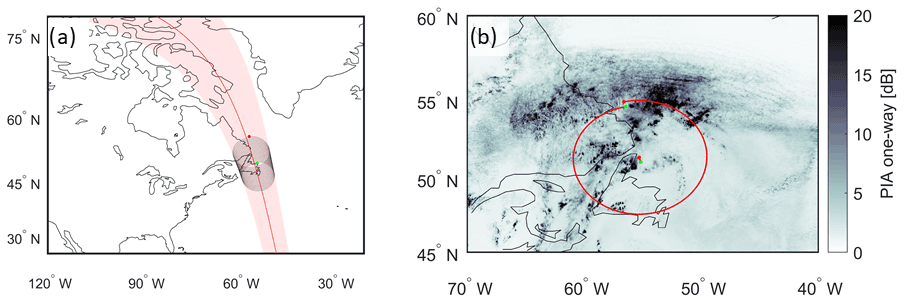
Figure 9 (a) WIVERN satellite track off the Labrador coast with the satellite ground track (red line), the scanning swath (shaded red region), and the radar footprints (black line) for 20 full revolutions of the conically scanning antenna corresponding to a flight time of 100 s. (b) Details of a single revolution of the WIVERN antenna with the one-way path integrated attenuation due to the hydrometeors shown in the background. This rotation sample will be examined in detail later (see Figs. 12–15).

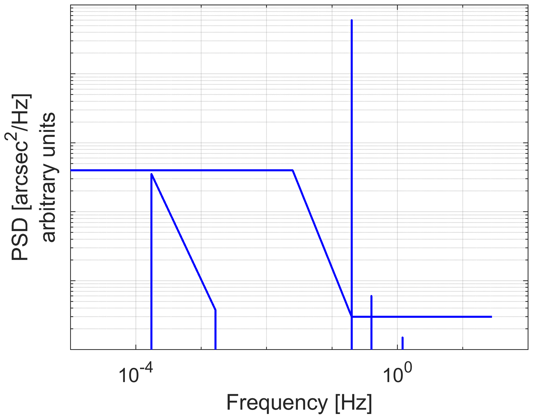
Figure 10 Conceptual model of the azimuth absolute knowledge error PSD. Contributions from different mechanisms are expected in different regions of the spectrum. For instance, sharp peaks are expected in correspondence to the scan harmonics.

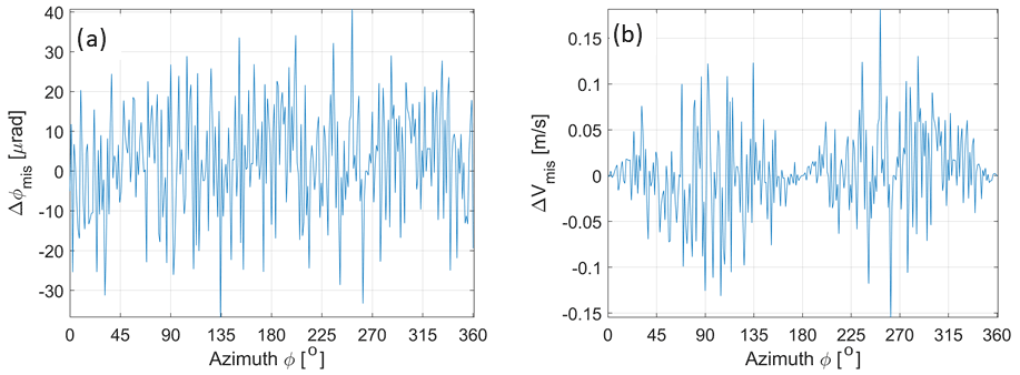
Figure 11 (a) One possible time series of the azimuthal scanning angle mispointing corresponding to a PSD, like in Fig. 10, as provided by preliminary industrial studies. (b) LOS velocity error corresponding to the mispointing shown in panel (a). Mispointing errors corresponding to the PSD in Fig. 10 are generally smaller than 0.1 m s⁻¹, far lower than the precision of the Doppler velocity observations.

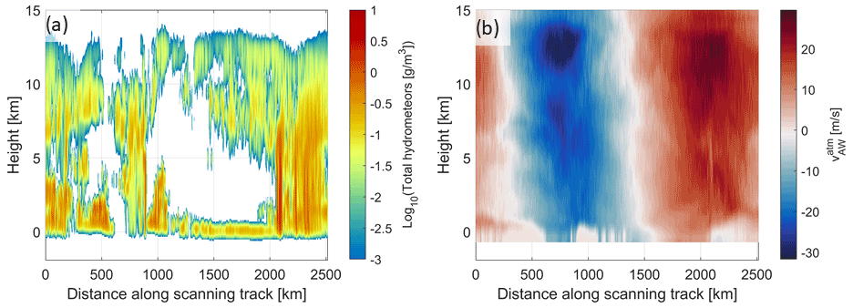
Figure 12 Antenna weighted hydrometeor content in grams per cubic meter (g m⁻³) expressed in base 10 logarithmic scale (a) and LOS winds (b) in correspondence to the revolution shown in Fig. 9b. Only hydrometeor contents above 1 mg m⁻³ are shown. The change in velocity reflects the different antenna viewing directions of the weather system.

Figure 13 Atmospheric (a) and surface (c) reflectivities and Doppler velocities (b, d) in correspondence to the revolution shown in Fig. 9b as a function of the distance along the scanning track. In order to facilitate the interpretation, we have added color bars above the top panels to indicate the surface type (green for land, blue for ocean, and brown for coasts) and above the bottom panels labels, indicating the azimuth position angle ϕ (measured clockwise and equal to zero when the antenna is looking forward along the traveling direction; see Fig. 5). For the velocity panels, we have used a yellow background in correspondence to low SNR regions for clarity of display. The reflectivity (a) clearly shows regions of high attenuation below the freezing level altitude (located at about 4.5 km), especially in correspondence to distances along the scanning track between 2200 and 2300 km. In that region, the attenuation is so high that the surface contribution is well below the radar sensitivity (c). In the lower panels, the surface contributions are shown in the ±1 km altitude region. Note that the ground clutter for the 500 m long pulse is higher over the land than over the sea and higher in regions with no attenuation (c).

Reflectivities and mean Doppler velocities for the atmospheric and surface targets computed, according to the methodology described in Sect. 2.3.1, are shown in Fig. 13. The atmospheric reflectivity mirrors the hydrometeor contents but with a region of strong attenuation corresponding to heavy rain from 2000 km onward. Only reflectivities above −30 dBZ are shown. The surface reflectivity and Doppler velocities are shown in the bottom panels. The reflectivity of the surface is clearly modulated by two effects, i.e., atmospheric attenuation (very strong, e.g., between 2050 and 2100 km in the along-track coordinate) and σ₀ variability with large discontinuities at sea–land transitions (e.g., at about 670, 805, and 1390 km in the along-track coordinate). Note that the clutter signal tends to decrease to very low levels ($<-\mathrm{30}$ dBZ) at a height of 1 km. This confirms previous findings (Illingworth et al., 2020). However, in future work, attention should be paid to antenna sidelobes that can effectively enhance clutter contamination on Doppler velocity signal, especially over land (see Illingworth et al., 2020, Fig. 8).

The surface Doppler velocities, sampled at very fine range resolution (Fig. 13d), show their characteristic behavior with zero velocity at the surface range (the satellite velocity along the antenna boresight is always subtracted out) and a pattern of positive and negative velocities at other ranges, with a strong dependence on the scanning azimuthal angle, which is used as an alternative x-axis coordinate in Fig. 13d. Note that the surface Doppler velocities are always zero at the surface ranges because the surface is assumed to be still. The azimuthal angle is measured clockwise from the forward-looking direction (where it is in the same direction as the satellite motion). When the radar is side-looking, the surface appears perfectly still at all altitudes, whereas, when the radar is looking in the forward or backward directions, there is a strong variability with altitude. As a result, the bias in Doppler velocities induced by clutter contamination will depend on the signal-to-clutter ratio, the altitude, and the azimuthal scanning direction. Overall, when averaging over heights and azimuthal angles, the clutter contamination will produce a bias towards zero Doppler velocities, i.e., the ground clutter will tend to mute the boundary layer winds.

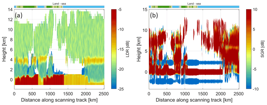
Figure 14 Linear depolarization ratio (LDR; a) and signal to ghost (SGR; b) in correspondence to the revolution shown in Fig. 9b as a function of height. The LDR clearly shows the significant depolarizations by the melting layer that is straddling the heights around 4 km and by the surfaces with clear transitions from strong depolarizing land to weaker depolarizing sea surfaces. At ranges where ghost but no real clouds are present, the SGR becomes −∞ in logarithmic units (zero in linear units); thus, the SGR is capped at −10 dB. This is the case for several instances at a height of ±2.3 (which corresponds to a slant range of 3 km) in coincidence with surface cross-talk.

The LDR values shown in Fig. 14a clearly have the highest values in the melting layer and the land surfaces. These two regions are the major sources of ghosts, as can be deduced by looking at the SGR (Fig. 14b), with strongly negative values associated with the ghosts generated by the surface at heights straddling ±2.3 km and with larger SGRs at about 6 km associated with the ghosts caused by the melting layer. Ghosts also tend to appear at cloud top (see strongly negative SGRs in such regions in Fig. 14b), a phenomenon which, if not accounted for, will tend to artificially thicken high clouds.

Figure 15 Reflectivity and Doppler velocity results corresponding to a full revolution of the WIVERN antenna, as shown in Fig. 13, for an integration length of 1.0 km (M=8). (a) Simulations of the WIVERN reflectivities (signal and noise) with ghost echoes at 2.3 km above and below the ground due to the depolarization by the surface, leading to ghost echoes where there is no real cloud. (b) WIVERN retrieved line-of-sight Doppler velocities after performing the polarization diversity pulse pair processing. Black solid and green dashed contour lines correspond to Doppler velocity precision computed, according to Eq. (16), of 3 and 1.5 m s⁻¹, respectively. Note that the echoes contaminated by ghosts have lower precision.

The two panels of Fig. 15 show simulations of WIVERN products, i.e., reflectivities (Fig. 15a) and LOS Doppler velocities (Fig. 15b) after 1 km along-track integration. The reflectivities ($Z\left(r\right)=\mathrm{0.5}\left[Z_{\mathrm{1}}\right(r)+Z_{\mathrm{2}}(r\left)\right]$) are the averages of M=8 pairs and include signal and noise. At such an integration length, the sensitivity (after noise subtraction) is expected to be −22.5 dBZ, i.e., 5log ₁₀(8)=4.5 dB better than the single-pulse sensitivity. Only regions with signals exceeding this level are plotted in Fig. 15.

The presence of ghosts arising from surface cross-talk is obvious around an altitude of ±2.3 km. Because of the considerably higher ${\mathit{\sigma }}_{\mathrm{0}}^{HV}$ over land, the signal-to-ghost ratios defined as the minimum values between SGR₁ and SGR₂, as defined in Eq. (17), are significantly smaller over ocean than over land, where they almost disappear below the noise level (Fig. 14b). The ghosts only marginally affect the LOS velocities (Fig. 15b); they only cause an increase in the standard deviation of the Doppler velocities according to Eq. (16) in the regions with detectable signal. Velocities are limited to the Nyquist interval (−40, +40) m s⁻¹, which is broad enough to capture the maximum amplitude of the LOS winds in this scene (Fig. 12b). In regions with very low SNR or SGR (e.g., around −2.3 km below the surface), the estimated velocities practically become random numbers within the Nyquist interval (hence the grainy texture in the graph). Otherwise, the estimated LOS Doppler velocities resemble the LOS winds depicted in Fig. 12b well, which is confirmed by the good precision of the winds always being better than 3 m s⁻¹ in regions of high SNR and by small biases introduced by NUBF and wind shear errors (see Sect. 3.2).

Another WIVERN product is the H- and V-polarized brightness temperatures (Fig. 16). Due to the difference in emissivities, there is a clear separation of the vertical- and horizontal-polarized brightness temperatures (T_B) over the ocean. With increasing optical thicknesses, the two T_B tend to become closer and closer. This T_B enhancement due to emission over cold backgrounds is expected to be useful for rain retrievals. In fact, because of the reduced and more variable ocean NRCS, surface-reference-technique-based path integrated attenuation (PIA; Meneghini et al., 2021) estimates will be more challenging and more sparse in the WIVERN configuration than for nadir-looking radars. In addition, T_B are known to have a better sensitivity than PIAs (Battaglia et al., 2020a), i.e., they will produce a detectable signal at smaller optical thicknesses (compare blue and red line variability). The coincident sampling of reflectivity profiles and T_B will be unique and provide insights into supercooled cloud liquid water coexisting with snow over the ice-free ocean (Battaglia and Panegrossi, 2020) and the evolution of large ice particles in deep convection.

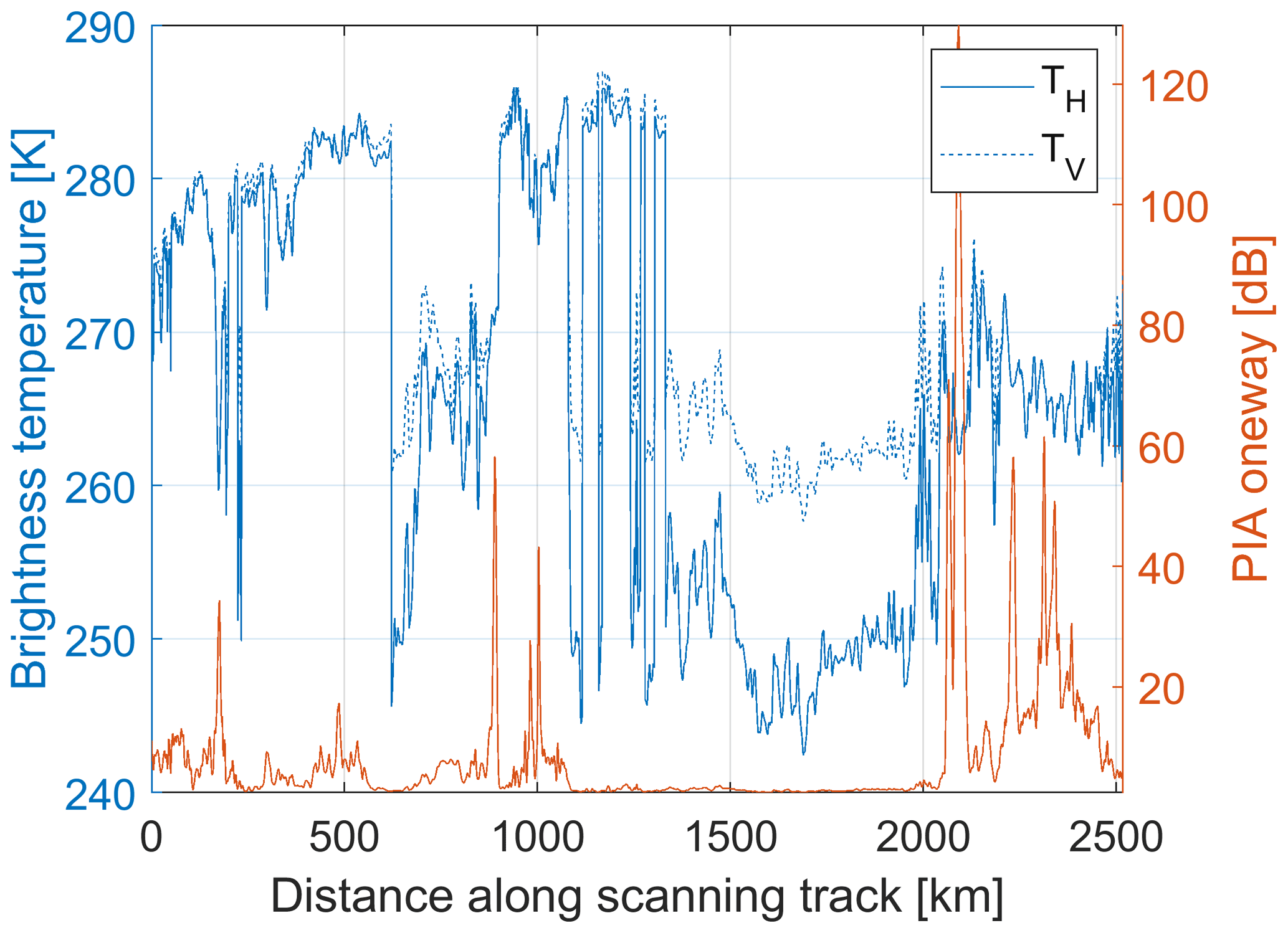
Figure 16 Simulated brightness temperatures for V (continuous blue) and H (dashed blue) polarization. For clarity of presentation, we have not added the expected measurement noise. The total one-way PIA (red line) is also given for reference. Results correspond to a full revolution of the WIVERN antenna, as shown in Fig. 13.

3.2 WIVERN performance assessment

The E2E simulator represents a useful tool for studying the performances of the WIVERN mission. Apart from the errors related to the Doppler estimators in the pulse pair processing (Eq. 16) and the mispointing (Tanelli et al., 2005), there are other sources of uncertainties in polarization diversity Doppler radar measurements, such as errors linked to wind shear either associated with the platform motion (Tanelli et al., 2002; Kollias et al., 2014) or the atmospheric winds (Battaglia et al., 2018), to clutter contamination (Illingworth et al., 2020), and to aliasing (Battaglia et al., 2013; Sy et al., 2014). The contribution of each of these errors can be quantified unambiguously by running two simulations where the effect is turned on and off.

3.2.1 Wind shear errors

The wind shear errors which tend to occur when reflectivity and velocity gradients are present at the same time within the backscattering volume, as can happen at the boundaries of clouds, can be computed from the difference between v_AW in Eq. (19) and the expression of $v_{\mathrm{D}}^{\mathrm{atm}}$ in Eq. (14) with v_sat set to 0. Results are shown in Fig. 17a in correspondence to the revolution shown in Fig. 9b. Strong wind shears appear in this case at near-surface altitudes (see Fig. 12b). This results in significant wind shear errors exceeding ±1 m s⁻¹, affecting the measurements at the low altitudes, but Fig. 17 shows that these errors impact only limited regions and are close to zero for most areas within the observed scene.

Figure 17 Errors induced by wind shear (a) and NUBF (b) in correspondence to the revolution shown in Fig. 9b. After corrections for beam filling using the vertical gradient of Z derived from the WIVERN data itself, these errors are expected to reduce to less than 1 m s⁻¹.

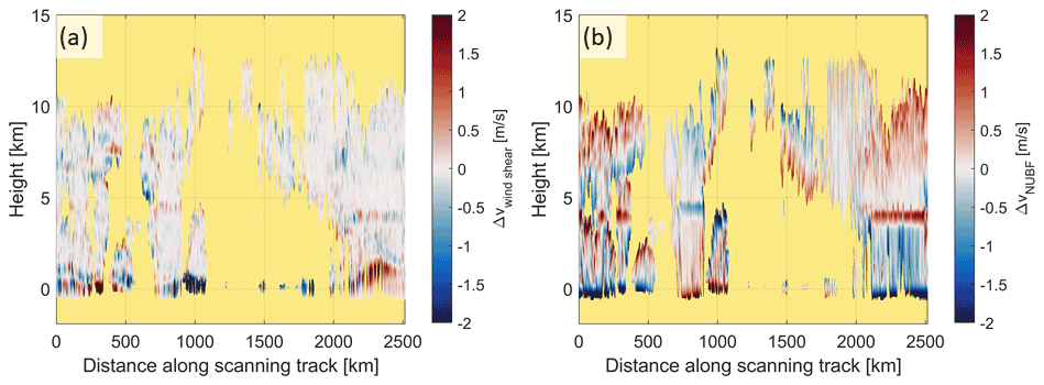
3.2.2 Non-uniform beam filling: satellite-motion-induced biases

Estimates of the NUBF errors can be obtained by comparing the expression of $v_{\mathrm{D}}^{\mathrm{atm}}$ in Eq. (14) with and without v_sat set to 0. Because of the different directions of the satellite velocity with respect to the antenna boresight when changing the scanning position, the NUBF errors depend on the azimuth scanning angle. The satellite velocity produces an apparent wind shear across the backscattering volume, with velocities ranging from −3.4 (−4.4) to +3.4 (4.4) m s⁻¹ at forward-/backward-(side-)looking configurations across the 3 dB WIVERN footprint. When coupled with a reflectivity gradient (computed along the direction orthogonal to the boresight and lying in the plane generated by the satellite velocity and by the antenna boresight; Battaglia et al., 2013), this satellite-motion-induced velocity shear will produce a NUBF bias. Figure 17b shows NUBF errors for the revolution of Fig. 9b and clearly demonstrates that the effect can be of several meters per second (m s⁻¹), is strongly azimuth angle dependent (typically minimized at side view, e.g., for a distance along the scanning track of about 625 and 1250 km), and is driven by vertical gradients (e.g., strongly enhanced at the cloud top and in the melting layer). We have computed NUBF statistics for 20 full revolutions (i.e., a distance along the scanning track exceeding 50 000 km) over the Labrador scene depicted in Fig. 9a. The distribution of the NUBF Doppler velocity biases as a function of the azimuthal scanning angle is shown in Fig. 18. In general, the effect is maximum in the forward and backward directions (ϕ=0^∘, 180^∘) because in these directions the error is partly coupled with the vertical gradients of reflectivity. As a result, opposite biases are generally present in the upper troposphere and in the bright band (where Z is sharply decreasing with height) and in the lower troposphere where, due to attenuation, reflectivities are increasing with height. At the side view (ϕ=90^∘, 270^∘), the error is coupled only with the horizontal gradients of reflectivity, which may not be well captured by the model due to its coarse horizontal resolution. Thus, NUBF errors may be underestimated by our simulations at the side view. Overall, NUBF errors are within the requirements with the 10th and 90th percentiles, exceeding 2 m s⁻¹ only at backward and forward viewing. Due to the conically scanning symmetry, NUBF errors are equal and opposite when considering corresponding scanning directions in the forward and backward segment of the scan. When averaging winds over spatial scales of the order of 20 km or more (see Table 1), this will practically eliminate the NUBF bias and only worsen the precision of the LOS winds.

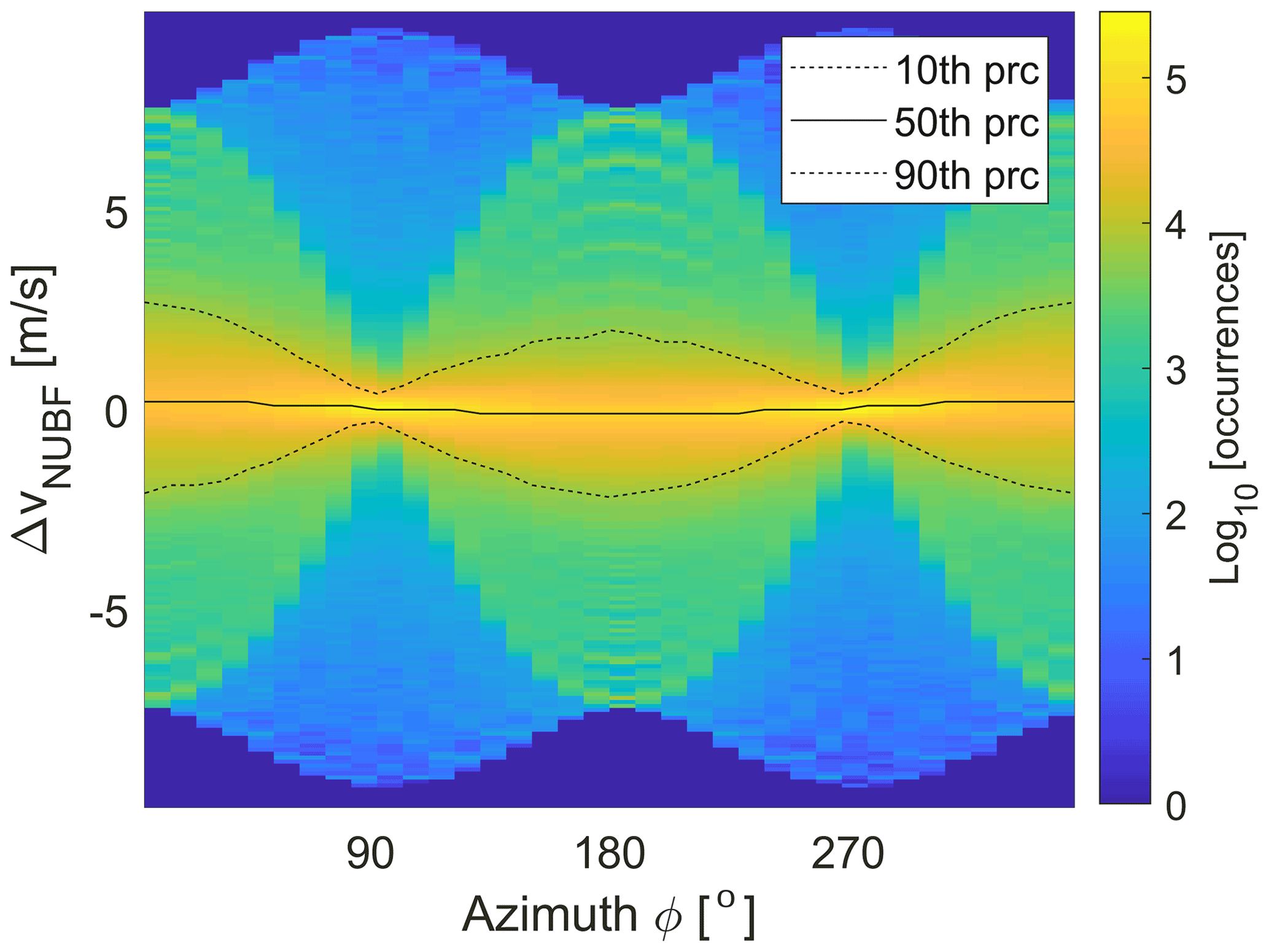
Figure 18 Histogram of NUBF-induced error as a function of the azimuthal scanning angle. The color indicates the log ₁₀ of the number of occurrences. The statistics are computed for 20 full rotations over the scene depicted in Figs. 12–15. The dotted lines represent the 10th and 90th percentile (typically with absolute value lower than 2.0 m s⁻¹), whereas the continuous line corresponds to the median value (always very close to zero because many NUBF errors are equal in magnitude and opposite in sign so will tend to cancel out).

4 Conclusions and future work

This study introduces a state-of-the-art E2E simulator tailored to simulating space-borne conically scanning Doppler radars adopting polarization diversity with the inclusion of a radiometric mode. The WIVERN configuration, as proposed to the ESA Earth Explorer 11 call (see specifics in Table 3), has been implemented in this study. The simulator reproduces the satellite orbit, the radar scanning geometry, and the illumination of an atmospheric scene extracted from a global atmospheric circulation model providing fine-resolution vertical profiles of winds and clouds. The coupling between the orbit and the atmospheric model allows global-scale simulations of mission observables, i.e., reflectivities and Doppler velocities of atmospheric targets. In addition, surface modeling accounts for the clutter returns from land and sea surfaces. The simulator also outputs estimates of Doppler measurement errors, such as those due to intrinsic noise, to cross-talk noise between the two diversely polarized channels, and to those introduced in presence of reflectivity gradients (wind shear and non-uniform beam-filling errors). Additional disturbances originate from the antenna azimuthal mispointing errors, which are represented in terms of an absolute knowledge error power spectrum.

Preliminary findings show that mispointing errors associated with the antenna azimuthal mispointing are expected to be lower than 0.3 m s⁻¹ (and strongly dependent on the antenna azimuthal scanning angle), wind shear and non-uniform beam-filling errors generally have negligible biases when full antenna revolutions are considered, NUBF causes random errors strongly dependent on the antenna azimuthal scanning angle but typically lower than 1 m s⁻¹, and cross-talk effects are easily predictable so that areas affected by strong cross-talk noise can be flagged. The noise random errors are dependent on the SNR and the possible presence of ghosts and can be reduced by averaging over a higher number of pulses (i.e., by using a longer integration time). In summary, our results show that the quality of the Doppler velocities appears to strongly depend on several factors, such as the strength of the cloud reflectivity, the antenna-pointing direction relative to the satellite motion, the presence of strong reflectivity and/or wind gradients, and the strength of the surface clutter. Overall, the E2E simulations suggest that total wind errors meet the mission requirements in a good portion to the clouds detected by the WIVERN radar, which is a very encouraging finding at the beginning of the Phase 0 studies.

The characterization of the errors and the isolation of each single error source makes the E2E simulator a useful tool to verify mission performances and compliance with requirements, which will be part of the Phase 0 studies that started in December 2021 and due to end in October 2023. Different problematic areas will be investigated with the introduction of new features (see Table 2).

1. By changing the antenna gain (Eq. 1), it will be possible to study the impact of antenna side lobes in affecting the minimum height close to the surface at which winds can be observed by the WIVERN radar without suffering significant biases from the clutter return.

2. More sophisticated surface modeling could be introduced by including the dependence on the surface winds over the ocean and different surface types over land.

3. Cloud scenes at finer horizontal resolution (≲1 km) that resolve convection could be used in the simulator at a regional (if not global) scale; this will enable us to evaluate WIVERN performances in the presence of convective motions.

4. A multiple scattering module, based on the two-stream approximation (Hogan and Battaglia, 2008), could be applied to the 1D WIVERN slant column and used to flag multiple scattering contaminated profiles in regions of deep convection.

5. Additional polarimetric variables like specific differential phase (K_DP), specific differential attenuation (A_DP), and cross-correlation (ρ_hv) could be simulated. This requires fundamental changes in the scattering look-up tables and in introducing polarization dependency in all variables.

6. Further studies on mispointing effects will be performed once power spectral densities of azimuth and elevation knowledge error are better specified by industrial studies. In particular, the E2E simulator will be able to assess how frequently and with which accuracy the surface return could be used to check the elevation pointing.

7. The E2E simulator will also serve as the basis to develop mitigation algorithms for NUBF, wind shear, mispointing, and vertical wind corrections that will be needed in order to produce horizontal line of sight winds, which will be the product directly assimilated by numerical weather prediction models.

Thanks to its modular structure, the simulator can be easily adapted to different orbits, a gamut of scanning geometries (e.g., cross-track), and various frequencies (by simply changing the look-up tables). Therefore, the simulator could be applied to simulate other space-borne Doppler atmospheric radars as well.