the Creative Commons Attribution 4.0 License.
the Creative Commons Attribution 4.0 License.
 | 18 May 2022
Homogenization of the Observatoire de Haute Provence electrochemical concentration cell (ECC) ozonesonde data record: comparison with lidar and satellite observations
Gérard Ancellet
Sophie Godin-Beekmann
Herman G. J. Smit
Ryan M. Stauffer
Roeland Van Malderen
Renaud Bodichon
Andrea Pazmiño
The Observatoire de Haute Provence (OHP) weekly electrochemical concentration cell (ECC) ozonesonde data have been homogenized for the period 1991–2021 according to the recommendations of the Ozonesonde Data Quality Assessment (O3S-DQA) panel. The assessment of the ECC homogenization benefit has been carried out using comparisons with other ozone-measuring ground-based instruments at the same station (lidar, surface measurements) and with colocated satellite observations of the O3 vertical profile by Microwave Limb Sounder (MLS). The major differences between uncorrected and homogenized ECC data are related to a change of ozonesonde type in 1997, removal of the pressure dependency of the ECC background current and correction of internal pump temperature. The original 3–4 ppbv positive bias between ECC and lidar in the troposphere is corrected with the homogenization. The ECC 30-year trends of the seasonally adjusted ozone concentrations are also significantly improved in both the troposphere and the stratosphere after the ECC homogenization, as shown by the ECC/lidar or ECC/surface ozone trend comparisons. A −0.19 % yr−1 negative trend of the normalization factor (NT) calculated using independent measurements of the total ozone column (TOC) at OHP disappears after homogenization of the ECC data. There is, however, a remaining −3.7 % negative bias in the TOC which is likely related to an underestimate of the ECC concentrations in the stratosphere above 50 hPa. Differences between TOC measured by homogenized ECC and satellite observations show a smaller bias of −1 %. Comparisons between homogenized ECC and OHP stratospheric lidar and MLS observations below 26 km are slightly negative (−2 %) or positive (+2 %), respectively. The comparisons with both lidar and satellite observations suggest that homogenization increases the negative bias of the ECC to values lower than −6 % above 28 km. The reason for this bias is still unclear, but a possible explanation might be related to freezing or evaporation of the sonde solution in the stratosphere.
- Article
(2730 KB) - Full-text XML
- BibTeX
- EndNote


Stratospheric ozone recovery is expected due to decreasing atmospheric amounts of ozone-depleting substances. Trends of ozone in the upper troposphere and lower and mid stratosphere, however, show latitudinal and seasonal variabilities which depend on (i) dynamical variability of the atmosphere, (ii) the temperature dependence of stratospheric ozone photochemistry and (iii) the increase of tropospheric ozone precursors in the upper troposphere (Szelag et al., 2020; Cohen et al., 2018; Thompson et al., 2021). A large number of validation and intercomparison studies of free tropospheric and lower stratospheric ozone use balloon-borne electrochemical concentration cells (ECCs) as reference (Tarasick et al., 2021). At Observatoire de Haute Provence (OHP), stratospheric and free tropospheric ozone monitoring is carried out since the mid-1980s with ozonesonde and lidar observations. The OHP station, located at 44∘ N, 6∘ E, is one of the few long-term measuring stations for vertical ozone profiles in southern Europe. This station allows for the characterization of (i) the impact of ozone sources observed in one of the hot spots of high tropospheric ozone column amounts observed by satellite (Richards et al., 2013) and (ii) the effects of climate variability on midlatitude total column ozone (Zhang et al., 2015; Petkov et al., 2014). Improvement and homogenization of the OHP ozone ECC observations have been achieved from 1991 to 2021 using the recent Ozonesonde Data Quality Assessment (O3S-DQA) panel recommendations (Smit et al., 2012; Smit and Thompson, 2021). An extensive use of lidar measurements both at tropospheric and stratospheric altitudes together with colocated satellite observations obtained during the OHP ECC soundings has allowed for the quantification of the ozone measurement improvement achieved with this homogenization of the ECC ozonesondes. Sections 2 and 3 summarize the corrections made to the ozonesonde measurements and the methodology for assessing its benefit. Section 4 presents and discusses the results of the different instrumental comparisons and the changes obtained in terms of interannual ozone variation at different altitudes between 0.7 and 30
A total number of 1412 ECC ozonesondes (Ancellet, 2021) have been launched at OHP since 1991 when Brewer–Mast regular soundings have been replaced by ECC sondes following the preparation instructions of Komhyr (1986) just after a lidar/ozonesonde intercomparison campaign held at OHP in 1989 (Beekmann et al., 1994). Ozonesondes are launched once a week generally around 09:00 UT, but 40 soundings have been made during the night either for lidar/ozonesonde comparison or for detection of long-range transport of polar ozone streamers forecasted by chemical transport models. The ozone partial pressure (measured in mPa) by the ECC can be obtained from the electrochemical current I (measured in µA), the background current Ib measured in the preparation laboratory with an ozone removal filter after the sonde was exposed to ozone, the internal temperature of the air sample Ti (in K), the capture efficiency of the O3 in the liquid phase α, the stoichiometry S of the O3 to I2 conversion, and the ECC pump flow rate ϕp (in cm3 s−1) (Smit and Thompson, 2021).
A major change in the sounding procedure occurred in 1997 when the Science Pump Corporation (SPC) ozonesonde was replaced by an EnSci ozonesonde while using a sensing solution type (SST) of 1 % (1 % KI concentration and a full buffer concentration; Smit and Thompson, 2021). Using the instructions given by the O3S-DQA, the following corrections have been implemented in Eq. (1):
-
Change of α and its pressure dependency before 1996 when 2.5 cm3 of KI solution was used in the cell instead of the recommended 3 cm3.
-
Scaling of measured by the EnSci-SST 1 % ozonesondes after March 1997 to from SPC-SST 1 % ozonesonde observations made before March 1997, assuming that SPC-SST 1 % is a better reference than EnSci-SST 1 % (Deshler et al., 2017). This correction is larger than −10 % at altitudes above 30 km and on the order of −4 % in the troposphere.
-
When Ib> 0.1 µA (less than 6 % of the dataset), Ib is replaced by 0.05 µA, the average of the measured background current for our dataset, while the uncertainty of Ib becomes 0.1 µA.
-
The pressure dependency of the background current was removed for the homogenized version since the O2 concentration does not play a significant role in the residual current when ozone is removed (Thornton and Niazy, 1983; Vömel and Diaz, 2010).
-
No vertical smoothing of the ozone partial pressure. Smoothing over 100 m was applied in the uncorrected data, i.e., before homogenization.
-
Correction of measured Ti to account for changes in the position of the thermistor and for differences with the true air sample temperature (the thermistor was taped to the pump before July 2007 and inserted in the pump hole since that time).
-
Correction of the pump flow rate to account for the humidification effect when using the bubble flowmeter to determine the flow rate in the laboratory as part of the pre-flight preparation of the sonde.
-
Two different correction tables of the pump flow rate efficiency at pressures below 100 hPa are now applied for EnSci (Komhyr95) and SPC (Komhyr86) ozonesonde. Komhyr86 was applied for the current to conversion of all the uncorrected data.
As the background current uncertainty is a significant contribution to the uncertainty in the upper troposphere (Van Malderen et al., 2016), the comparison of Ib used before and after homogenization is shown in Fig. 1. The standard deviation of the background current between 1991 and 2021 remains on the order of ±0.05, and only 17 % of the Ib values are greater than the mean of the uncorrected Ib after homogenization. The removal of the pressure dependency of the background current leads to significant relative differences (>5 %) in the upper troposphere where the ECC current is smallest. In February 2004, the UHF receiver and ground calibration tools were changed, and a new processing software, STRATO, developed by Holger Vömel at NOAA (https://cires1.colorado.edu/~voemel/strato/strato.html, last access: 9 May 2022) was implemented for the O3 partial pressure retrieval. The raw ECC current data files for between February 2004 and July 2007 no longer exist, and the ECC currents have been retrieved from the uncorrected ozone partial pressure using Eq. (1). The recorded lab temperature and relative humidity are used for the pump flow rate correction of ozonesondes launched after June 1999 (except in 2002 and 2003); for the other dates, the monthly means of the lab temperature and relative humidity terms in the pump flow rate equation (Smit et al., 2012) are used.
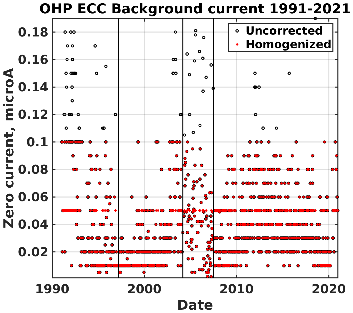
Figure 1Time evolution of the OHP ECC background current from 1991 to 2021. The red crosses are the currents after homogenization and the black circle before. The black lines correspond to the major ozonesonde changes in 1997, 2004 and 2007 (see Fig. 2).
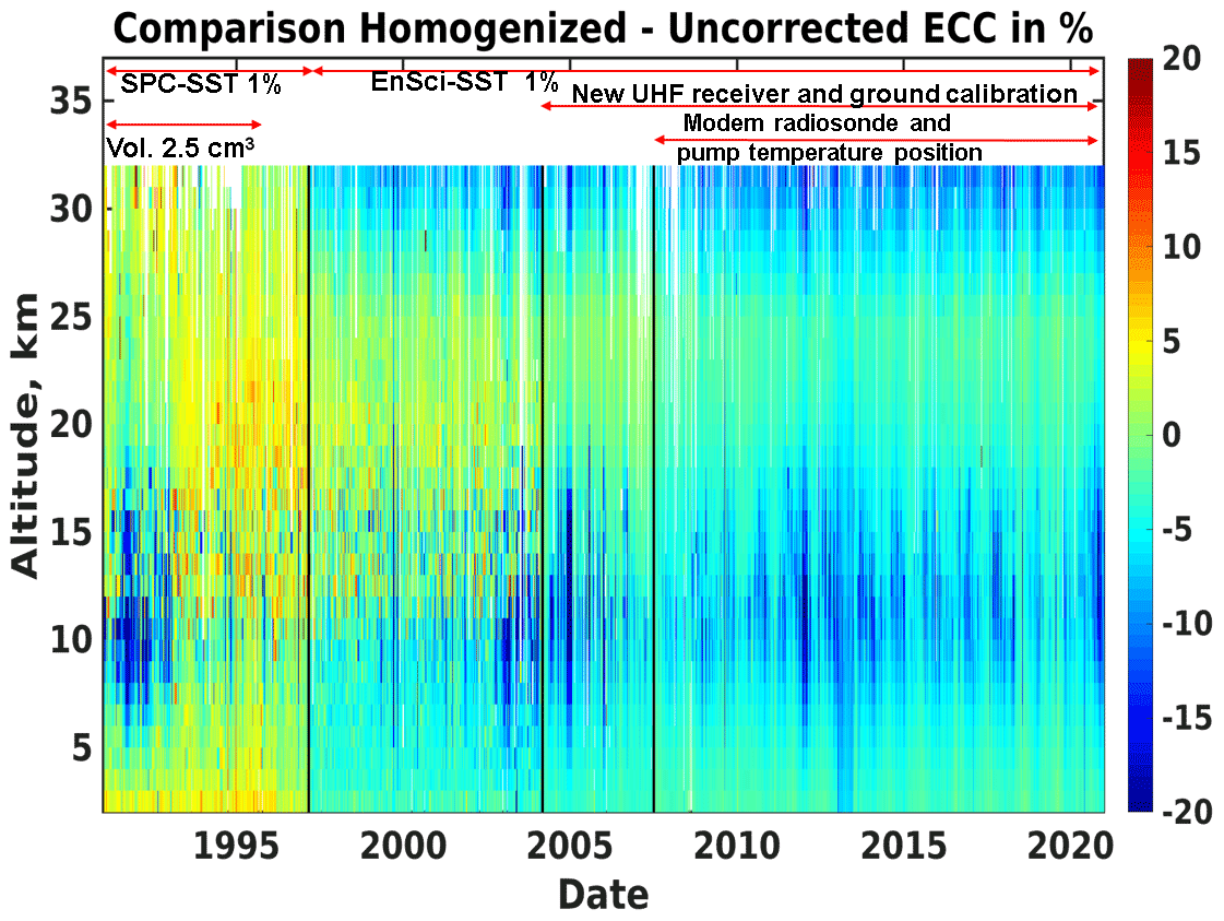
Figure 2Time evolution of the relative difference between homogenized and uncorrected ozone concentrations as a function of altitude. Color scale is in percent (%). Major changes in the sounding procedure or processing are shown in the top part of the figure. Pump flow rate corrections and removal of Ib pressure dependency are applied to the entire dataset.
In July 2007, the radiosonde type switched from Vaisala RS80 to MODEM M10. The MODEM M10 measures the true GPS altitude with the pressure altitude retrieved from this measurement. No correction is applied to the RS80 pressure measurements, and an offset of 0.5–1 hPa may exist in the stratospheric pressures above 20 km before 2007 (Tarasick et al., 2021; Stauffer et al., 2014).
The homogenized minus uncorrected ECC partial pressures normalized to the homogenized ECC ozone partial pressure are shown in Fig. 2. Significant overall negative differences ( %) are obtained (i) in the upper troposphere (8–12 km) because of the removal of Ib pressure dependency and (ii) above 28 km after 1997 when taking into account the change to EnSci. Positive differences reaching 5 % in the stratosphere are also observed for the SPC period before 1997 because of the positive corrections for the pump flow rate (+2 %) and the ECC pump temperature (+3 %) without any negative corrections in the stratosphere.
The UV–visible SAOZ (Système d'Analyse par Observation Zénithale) and the UV Dobson spectrophotometer total ozone column (TOC) measurements are available at OHP . The Dobson spectrophotometer was used from 1991 to 2004, and SAOZ data were used from 2004 up to now. The so-called normalization factor (NT) is calculated as the ratio of the spectrophotometer TOC and the ECC TOC. Following the methodology used in Smit and Thompson (2021) or Stauffer et al. (2020), the TOC corresponding to the ECC soundings is calculated using the integration of the ozone concentrations up to 10 hPa or the burst altitude, provided it is higher than 25 km. The residual ozone above 10 hPa or the burst altitude has been calculated using the monthly mean climatology of McPeters and Labow (2012) at pressures smaller than 10 hPa. The homogenized data are not normalized with this normalization factor, which is only used as a quality flag.
The homogenization procedure also includes a retrieval of the uncertainty in the ozone partial pressure at each vertical level. The detailed description of the uncertainty calculation is given in Smit and Thompson (2021). All the error terms have been included in our calculation except the bias due to the sensor time response and the pressure uncertainty. The median value of the relative uncertainty in the ozone concentration measured by the ECC is on the order of 6 %–7 % in the stratosphere and 7 %–9 % in the troposphere (see Sect. 4.2 showing the vertical distribution of the relative uncertainty of the ECC ozone concentrations used for the lidar–ECC comparisons).
In this work, the benefit from homogenization of the ECC ozonesonde time series is assessed by comparison of homogenized and non-homogenized ECC ozone concentrations with other ozone measurements carried out at OHP. First, these comparisons are made as a function of altitude using either Ultraviolet DIfferential Absorption Lidar (UV-DIAL) or Microwave Limb Sounder (MLS) satellite observations in the stratosphere (Froidevaux et al., 2008). Two UV-DIAL instruments have been operating at OHP. The first one, LiO3St, is optimized for stratospheric O3 profiling between 10 and 50 using an absorbed wavelength at 308 nm and a reference wavelength at 355 nm (Godin-Beekmann et al., 2002). The second one, LiO3Tr, is optimized for tropospheric ozone monitoring between 2.5 and 14 using the 289 and 316 nm wavelength pair (Ancellet and Beekmann, 1997). Regular nighttime measurements (2–4 per week) have been made with LiO3St since 1985 and with LiO3Tr since 1990. The LiO3Tr is most accurate in the 6–10 km altitude range with the smallest lidar systematic uncertainty (<8 %) due to the mismatch of the overlap function between the two wavelengths at ranges below 4 km and due to the background signal correction of the photomultipliers (PMT) nonlinear response above 10 km (Ancellet and Ravetta, 2003). The LiO3St best accuracy (≤5 %) is generally in the 15–40 km altitude range when ozone concentrations are large enough to minimize lidar systematic errors and when signal-to-noise ratio (SNR) is maximum (Nair et al., 2011). The uncertainty of the retrieved ozone concentration at each vertical level for LiO3Tr takes into account the statistical uncertainty due to the detection noise and the accuracy of the systematic error corrections. The following systematic errors have been taken into account: (i) the estimation of the time-dependent background signal and (ii) the residual error when correcting the effect of a differential overlap function at altitudes lower than 4 km. The retrieved ozone concentration accuracy for LiO3Str is calculated using the recommendations of Leblanc et al. (2016) not including a possible systematic error lower than 2 % due to the O3 absorption cross-section accuracy. To minimize the impact of spatiotemporal variability of ozone concentrations on the analysis of lidar–ozonesonde comparisons (Liu et al., 2013), nighttime soundings with a time lag of less than 2 or 6 h were considered in the troposphere or the stratosphere, respectively. We end up with a set of about 40 profiles for each lidar between 1994 and 2021. The time distribution of the number of lidar profiles per year for optimal comparison with ECC is shown for LiO3Tr and LiO3St in Fig. 3.
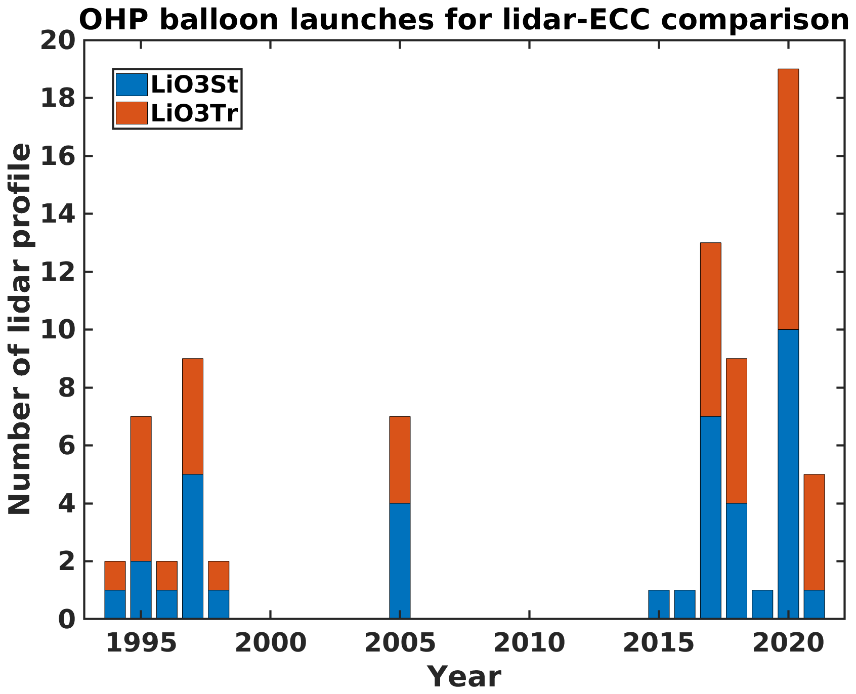
Figure 3Time distribution of the number of OHP lidar observations per year with a time lag between ECC launches and lidar measurement <2 h (LiO3Tr) or <6 h (LiO3St). These observations are used for the lidar–ECC comparison of Figs. 5 and 6. The blue bars correspond to LiO3St measurements and red bars to LiO3Tr.
The 2005–2021 stratospheric O3 profiles from AURA MLS v5 level-2 files have been also retrieved from 56.23 to 6.81 hPa with a vertical resolution on the order of 2 km at these levels (Schwartz et al., 2020). The overpass criteria are ±5∘ latitude and ±8∘ longitude, and all MLS profiles meeting this distance criteria within 1 d of the sonde are averaged to make the comparison with the ozonesonde. Although the spatiotemporal differences between ECC soundings and satellite overpasses will be greater using these criteria, we obtain many more comparisons than by restricting ourselves to nighttime soundings. For the sake of a more complete discussion of the two types of comparisons made in the stratosphere, we also considered a lidar dataset of 366 profiles from 2005 to 2021 with less restrictive measurement time difference with the ECC launches (<12 h). Such a criterion is valid as long as the rapid O3 variations typically encountered below 18 km are not present.
Secondly, comparisons of total ozone column (TOC) are also useful to check the benefit of the homogenization in the stratosphere. In addition to the TOC provided by the OHP spectrophotometer (Hendrick et al., 2011; Van Roozendael et al., 1998), satellite TOC level-2 (L2) overpass measurements by AURA Ozone Monitoring Instrument (OMI) (Bhartia, 2012), Suomi-NPP Ozone Mapping and Profiler Suite (OMPS) (Jaross, 2017), and Global Ozone Monitoring Experiment (GOME) 2A and B have been selected when they are within 12 h of the ozonesonde and selecting the closest pixel in time and space to the ozonesonde station. The vast majority of L2 TOC data are within 100 km of OHP. The corresponding ECC sounding TOC used for the satellite comparison is calculated using the integration of the ozone concentrations up to 10 hPa and the McPeters and Labow (2012) climatology above 10 hPa.
Thirdly, the benefit of homogenization on long-term ozone trends for several altitude ranges in the troposphere and the stratosphere has been studied using all the lidar and ECC measurements made at OHP. The lidar monitoring period is indeed as long as the ozonesonde dataset and includes the major ozonesonde preparation or ozonesonde type changes in 1997, 2004 and 2007. Only simple linear trends of the ozone concentrations corrected for the mean seasonal variation at OHP will be considered in this study. The trend uncertainties are calculated using the 95 % confidence limit of the slope of the linear regression, assuming that the residuals are not correlated for weekly (ECC) or per week (lidar) observations. A more comprehensive trend analysis for the OHP would need either a multiple linear regression model as described in Nair et al. (2013) or Thompson et al. (2021) for the stratosphere or a statistical regularization method as described in Chang et al. (2020) for the troposphere when data sampling is sparse. For the stratospheric trend, the period 1990–1995 is removed to minimize interferences by the eruption of Mt. Pinatubo. Lidar and satellite ozone observations cannot be retrieved in the lowest atmospheric layer below 2 ; O3 surface observations are then included using measurements of a TEI-49C instrument with an air intake on the roof of the lidar building. Data are recorded continuously since December 1997, except between June 2010 and August 2012 when the responsibility for surface ozone measurements was entrusted to the ATMOS-SUD air quality network at the same location. Data between July 2002 and July 2003 have also been removed because of a contamination problem in the air intake. The trend of O3 surface observations is compared to ECC trends using either all the daily mean O3 surface data available since 1998 or the hourly-mean O3 concentration measured on the day and time of the ECC launch. The correction of the corresponding mean seasonal variation is applied to both datasets. A significant difference between the two surface concentration trends might point towards a strong sensitivity of the trend sign to the limited number of observations by the ECC.
4.1 Normalization factor trend
The time evolution of the normalization factor NT is plotted in Fig. 4 for the uncorrected and homogenized OHP ECC sondes. The major changes in the ozonesonde supplier or the ozonesonde preparation procedure shown in Fig. 2 are also reported in Fig. 4. The uncorrected NT time evolution shows that the dispersion of points is larger before the switch to MODEM ozonesonde in 2007, but more striking is the significant negative trend of % yr−1 which is not negligible compared to the reported O3 trends in the troposphere (Gaudel et al., 2018). The homogenized NT does not exhibit a significant trend (0.02±0.03 % yr−1), indicating the strong benefit of the homogenization. However, the average normalization factor for the whole record increases from 1.019 to 1.037, corresponding to a −3.7 % bias of the ECC TOC compared to the OHP spectrophotometer. This may be partly due to the calculation of residual ozone above the burst altitude and partly to a possible bias in the stratosphere. The calculation of the residual ozone which accounts for 7 %–10 % of the ECC TOC leads to an uncertainty of about 1 % of the TOC according to Witte et al. (2018). A negative bias of about 3 % in the stratosphere is still necessary to explain an average normalization factor of 1.037.

Figure 4Time evolution of the OHP ECC normalization factor (NT) from 1991 to 2021 before (a) and after homogenization (b). The black lines correspond to the major ozonesonde changes in 1997, 2004 and 2007 (see Fig. 2). The thick blue lines are the 100-point, centered, moving averages. NT linear trends are shown in red, and the slope and its uncertainty with a 95 % confidence are given in percent per year (% yr−1).
4.2 Nighttime ozonesonde and lidar comparison
The ozone concentration vertical profiles of ECC ozonesondes launched within 2 h of the LiO3Tr observations have been divided into six 1.5 km vertical layers between 3 and 12 km. The relative differences between the ECC and lidar O3 concentration are calculated for each 1.5 km vertical bin. The means of the relative difference and its uncertainty are then calculated for the 40 profiles, and the time distribution of which is shown in Fig. 3. The uncertainty of the mean difference in a 1.5 km vertical interval for a single O3 profile is based on mean absolute uncertainties (systematic and statistical) of both lidar and ECC measurements (see Sects. 2 and 3) at each recorded altitude in the corresponding 1.5 km vertical interval. The statistical standard uncertainty of the overall, mean difference is then retrieved by assuming that the 40 comparisons are independent with uncorrelated uncertainties. The mean relative differences between the homogenized ECC and LiO3tr show an insignificant bias on the order of 1 % for the altitude range 4.5 to 9 km, considering the statistical standard uncertainty in this difference, which is on the order of ±2 % (Fig. 5a). The mean relative differences between the uncorrected ECC concentration and LiO3tr, however, show a significant bias on the order of +4 % in the same altitude range. They may be explained by differences introduced by not correcting the O3 partial pressure for EnSci-SST 1 % and by using a pressure-dependent background current subtraction. The comparison between the altitude dependence of the uncertainty of the lidar measurement and that of the ECC measurement in the troposphere (Fig. 5b) shows that the ECC uncertainty remains in the range 7 %–9 %, while the lidar is less accurate (uncertainty >9 %) below 4.5 km and above 11 km. Below 4 km the significant bias of −4 % between the homogenized ECC and the LiO3tr can then be explained by the large uncertainty in the O3 retrieval by the LiO3tr (>10 %) because of the sensitivity to the overlap function correction in this altitude range. Above 10 km, the large difference between lidar and ECC (≈10 %) is due to different spatial resolutions for the two measurements in a region with strong O3 vertical gradients and due to the increasing uncertainty of the LiO3tr measurements in the lowermost stratosphere.
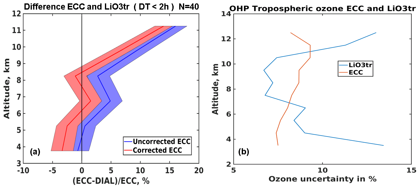
Figure 5(a) Mean relative ECC minus LiO3Tr ozone concentration differences (in %) between 3 and 12 km for uncorrected (blue) and homogenized (red) ozonesonde. Shaded areas represent the statistical standard uncertainty in the mean difference. (b) Vertical profiles of the median of the relative ozone concentration uncertainty in the troposphere for the homogenized ECC (red) and LiO3Tr (blue).
For the comparison with LiO3St, two time differences between ECC launch and lidar profiling period are considered: (i) 6 h for the 40 soundings shown in Fig. 3 and (ii) 12 h for 366 soundings made between 2005–2021 during the time period of the satellite measurements shown in Sect. 4.3. The means of the relative difference between ECC and LiO3St are then calculated for eight vertical layers between 14 and 30 km using the geometric altitude for the ECC sondes, as the geopotential altitudes become significantly larger than lidar geometrical altitudes above 25 km. As for the previous comparison with LiO3tr, the uncertainty of the mean difference between the two instruments is retrieved by assuming an independent error for the 40 or 366 comparisons taken into account. For the shorter time difference, the mean relative differences between the homogenized ECC and LiO3St still show a significant bias on the order of −3 % to −5 % between the ECC and LiO3St at altitudes between 18 and 28 km with an error on the mean difference which is on the order of ±1.5 % (Fig. 6a). Near 15 km, this difference decreases to less than 1 %. In contrast to the LiO3Tr comparison, the mean difference between the homogenized and uncorrected ECC measurements is small (≈2 %), except above 28 km where the homogenized ECC concentrations are even lower than the lidar concentrations by −8 % (Fig. 6a). For the period 2005–2021 and using a time difference less than 12 h, the negative bias between the homogenized ECC and the lidar decreases down to −2 % between 22 and 24 km but remains as large as −7 % above 28 km (Fig. 6b). Note also that the mean uncorrected ECC and lidar difference is now slightly positive (+1 %) for the 2005–2021 period in good agreement with the NT negative trend shown in Fig. 4. Below 18 km, the −4 % negative bias between homogenized ECC and lidar (Fig. 6b) should be interpreted by possible significant O3 concentration changes within 12 h in this altitude range. The time evolution of the relative difference of ECC and LiO3st ozone concentrations is shown in Fig. 6c and d for uncorrected and homogenized ECC, respectively. Many of the differences between uncorrected ECC and LiO3St are greater than +6 % between 2007 and 2016, while there are some negative differences approaching −6 % in 2006. Homogenization improves the relative differences, now remaining between −5 % and +5 %, except in 2006 when the negative bias decreases down to values smaller than −6 %. The comparison between the altitude dependence of the error of the lidar measurement and that of the ECC measurement in the stratosphere (Fig. 7) shows that the ECC error remains in the range 5.5 %–6.5 %, while the lidar is very accurate (error <2 %) between 18 and 30 km.
Considering that stratospheric lidar observations are highly accurate above 28 km, frequent freezing or evaporation of the ozonesonde sensing solution may explain the ECC low bias relative to the lidar above 28 km at OHP. The O3 partial pressure error related to a pressure offset for the Vaisala RS80 period may be another reason for the large difference with LiO3St ozone values, but this error will be limited as it exists for only one-third of the ECC sondes used for this comparison (25 MODEM and 15 RS80 radiosondes). When examining differences above 26 km between homogenized ECC and LiO3St for the MODEM and the RS80 subsets separately, there is indeed a larger negative bias of −4 % to −10 % for the RS80 compared to −6 % to −7 % for the MODEM. We have also considered two subsets with ECC pump temperature Ti at 30 km either higher or lower than 290 K. The negative bias between the homogenized ECC and LiO3St O3 concentrations above 26 km decreases down to −3 % for the high-Ti subset, while it ranges from −5 % to −7 % for the low-Ti subset. More investigations are needed to conclude that freezing or evaporation of the solution is indeed the major contributor to the negative bias of the ECC concentration measurements above 26 km.
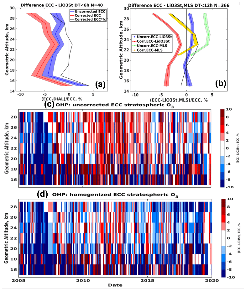
Figure 6Mean relative ECC minus LiO3St O3 concentration differences (in %) between 14 and 30 km for uncorrected (blue) and homogenized (red) ECC for (a) the 40 coincident (<6 h) profiles (see Fig. 3) and (b) the 366 profiles within 12 h during the MLS measurement period. Shaded areas represent the standard uncertainty in the mean difference. The solid black line shows the mean relative differences if the homogenized ECC concentrations are multiplied by NT. The mean relative ECC minus MLS O3 concentration differences are shown in (b) for uncorrected (green) and homogenized (yellow) ozonesonde. The time evolution of the relative ECC minus LiO3St O3 concentration differences (in %) are shown in (c) for uncorrected and (d) for homogenized ECC using the 366 profiles with a 12 h time difference.
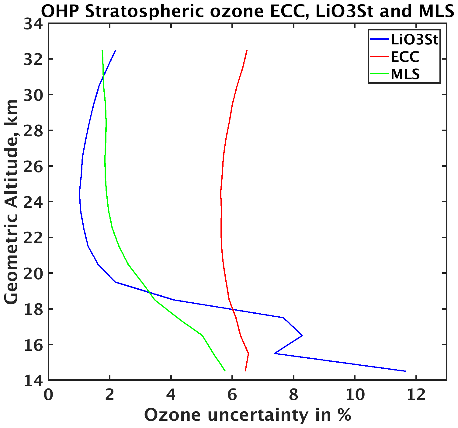
Figure 7Vertical profiles of the median of the relative ozone concentration overall uncertainty in the stratosphere for the homogenized ECC (red), LiO3St (blue) and MLS (green).
The −2 % to −4 % difference between LiO3St and the homogenized ECC in the altitude range 19–27 km even after homogenization is consistent with the mean normalization factor of 1.037 shown in Fig. 4. Indeed, the means of the relative difference between LiO3St and ECC are no longer significant below 28 km when the ECC concentrations are multiplied by the normalization factor (black curve in Fig. 6a). Note, however, that such a correction is not recommended for the ECC ozonesonde measurements (Smit and Thompson, 2021).
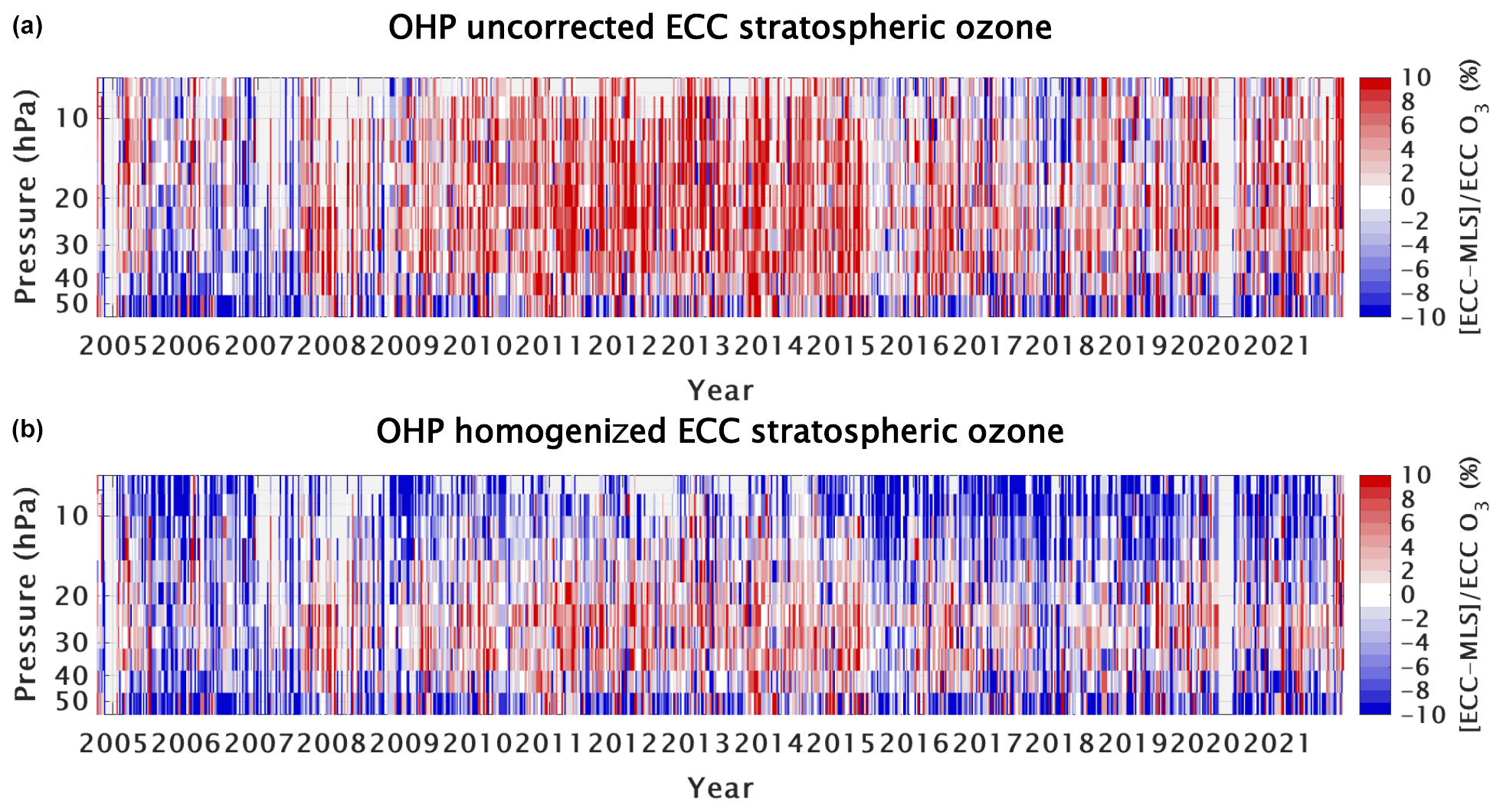
Figure 8Relative O3 concentration differences ECC minus MLS (in %) as a function of pressure between 50 and 7 hPa before (a) and after (b) homogenization.
4.3 Comparison of ozonesonde and satellite
The comparison of satellite and ECC measurements covers a period from 2005 to 2021. The vertical profiles of the relative differences of O3 concentrations between ECC and MLS are shown in Fig. 8 in the stratosphere from 20 km (50 hPa) to 31 km (10 hPa). The ozonesonde data are first averaged to 100 m vertical resolution and then interpolated onto the MLS pressure levels. While many differences exceed 5 % when the ECC data are uncorrected, especially between 2010 and 2015, the relative differences for the homogenized ECC data remain within the ±5 % interval. Above 28 km (15 hPa), we find a negative bias with values lower than −6 % when the ECC data are homogenized. An interesting feature of this MLS/ECC comparison is the interannual variability of the differences. It can be observed that differences using homogenized ECC data are more evenly distributed around zero. The same conclusion could be drawn from the time evolution of the relative differences between homogenized ECC and LiO3St presented in Fig. 6c and d. The fact that the average ECC-MLS difference shown in Fig. 6b is slightly positive (+2 %) in the 22–26 km altitude range while the average ECC–LiO3St difference is slightly negative (−2 %) means that homogenization is a good compromise for intercomparability with other techniques measuring O3 in the stratosphere below 26 km. Above 26 km, both comparisons indicate a negative bias in homogenized ECC O3 concentrations with values lower than −6 %.
The time distributions of differences between the ECC TOC and the satellite TOC are shown in Fig. 9. No filtering for clouds or distance is applied to have more comparisons available. The 100-point, centered, moving averages are superimposed on the set of data points corresponding to each single comparison. As expected, the results are consistent with comparison between ECC and stratospheric MLS profiles with the largest positive relative differences between uncorrected ECC and satellite TOC between 2010 and 2015. A small post-2013 drop-off in TOC measurement of −2 % by the ECC at OHP might be present, but this is considerably less prominent than the drop-off observed at other measurement sites in Stauffer et al. (2020). The uncorrected ECC and OMI/OMPS biases range between −1 % and +5 %, while it is between 0 and +3 % for GOME. Those differences are mostly negative and between −3 % and 1 % after homogenization. The ECC minus satellite TOC temporal evolution is consistent with the time distribution of the normalization factor shown in Fig. 4. However, TOC differences are close to zero between 2010 and 2016 using the satellite data, while a −3 % bias is present using the OHP total ozone measurement. In this context, we mention that the expected bias between GOME and SAOZ is between −3 % and +1 % (Hendrick et al., 2011).

Figure 9Relative differences ECC minus satellite total ozone column (in %) before (a) and after (b) homogenization. The thick lines are 100-point, centered, moving averages. No moving averages are plotted for less than 100 points.
4.4 Comparison of trend analysis
4.4.1 Surface trend
First, the interannual variation of homogenized and uncorrected ECC O3 concentrations have been retrieved in the lowermost troposphere (200 m layer above ground level) using the average ECC ozone concentrations in this layer. Such an interannual variation can be compared with the one deduced from the surface ozone measurements made since 1998. To quantify the 22-year trend of ozone mixing ratio associated with this interannual variation, the latter is deseasonalized by subtracting from the surface mixing ratios the monthly averages calculated over the 22 years of data. This removes a major source of O3 mixing ratio intra-annual variability which is on the order of 20 ppbv. The trends of the ozone mixing ratio and their 95 % confidence interval estimates are calculated using the regression lines across all the available deseasonalized mixing ratios. A weak negative trend on the order of ppbv per decade is obtained for the uncorrected ECC deseasonalized mixing ratio (called ozone anomalies hereafter), and this trend changes very little ( ppbv per decade) after homogenization of the ECC (Fig. 10). The ECC negative ozone trends compare very well with those obtained from surface measurements using either all the O3 daily means between 1998 and 2021 ( ppbv per decade) or only the hourly means for ECC launching times ( ppbv per decade). The small difference between the trend calculated for all the surface daily means available and the trend using only the ECC launching times shows that the sensitivity of the trend magnitude to the sampling by ECC is not so large. The negligible difference between the uncorrected ECC trend and the homogenized ECC trend near the surface is mainly due to the fact that identical corrections are applied for all the data in the 1998–2021 period, namely, (i) the scaling of EnSci-SST 1 % response to the SPC-SST 1 %, (ii) the pump flow rate correction and (iii) the removal of Ib pressure dependency. However, the difference of 11.2 ppbv between the 2003 positive yearly average of ozone anomalies and the 2005–2008 negative yearly anomalies for the uncorrected ECC (Fig. 10) is slightly reduced to 7.8 ppbv for the homogenized ECC (Fig. 10). The difference between the positive 2003 yearly average of ozone anomalies and the negative one for 2008 does not exceed 8 ppbv for the surface measurements (Fig. 10) and are, therefore, in better agreement with the homogenized ECC interannual variations.
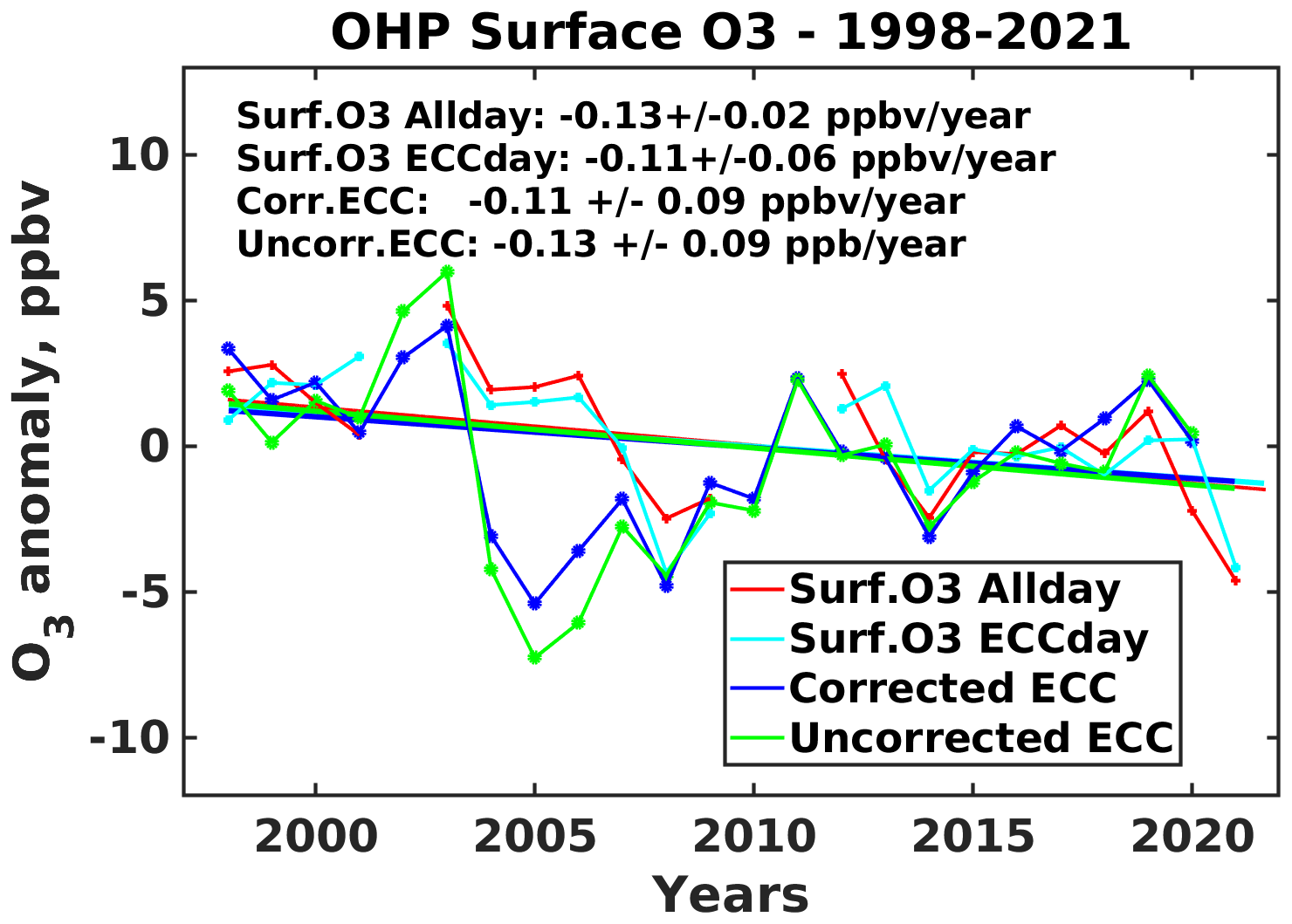
Figure 10Interannual variation of deseasonalized O3 mixing ratios (in ppbv) for the uncorrected ECC (green), homogenized ECC (blue) and daily mean observations of the OHP surface O3 analyzer. The ECC mixing ratios are averaged in the 0.2 km layer above the surface. The surface daily-mean observations are calculated when available (red) or for ECC launching days only (cyan). The corresponding regression lines through all the O3 anomalies between 1998 and 2021, O3 trends (in ppbv yr−1) and their uncertainties with a 95 % confidence are also shown.
4.4.2 Tropospheric trend
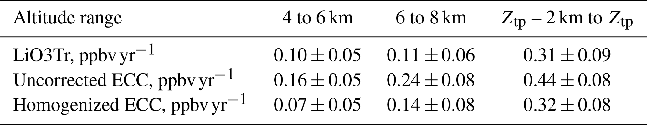
In this section, the interannual variation of homogenized and uncorrected ECC ozone data is compared in the free troposphere for three layers of 2 km thickness at 5 and 7 km and just below the dynamical tropopause taken at 2 Potential Vorticity units (PVu) (Fig. 11). The three layers were selected in order to compare the ozone trends of the ECC sondes with those of the LiO3tr lidar. The altitude Ztp of the dynamical tropopause is calculated using ECMWF meteorological analysis with 1∘ horizontal resolution and 137 vertical levels. The mean value of Ztp is 10.5 km at OHP (10 km in winter and 11.5 km in summer), so the upper layer approximately corresponds to the 8–10 km altitude range. As for the surface trend retrieval, the mean ozone concentrations of the layers are deseasonalized before calculating the trends of mixing ratios from the regression lines across all the 2 km ozone mixing ratio averages available in the 30-year database. The uncorrected ECC trends are always positive and significant, and they increase with altitude, with the largest value (4.4±0.8 ppbv per decade) in the layer below the tropopause (Table 1). The lidar measurements also show significant positive trends for the three layers but with smaller values, e.g., 3.1±0.9 ppbv per decade below the tropopause. The lidar trends are in better agreement with the trends calculated using the homogenized values, e.g., 3.2±0.8 ppbv per decade below the tropopause. Although the lidar and homogenized ECC yearly average of ozone anomalies are not similar from year to year considering the sampling differences, the main decennial changes are seen by both instruments above 6 km, namely, the sign change of the anomalies between the period 2000–2010 (positive) and 2010–2020 (negative) (Fig. 11). Overall, the homogenization greatly improved the ECC tropospheric trend retrieval with smaller and more realistic values.

Figure 11Interannual variation of deseasonalized O3 mixing ratios (in ppbv) for the uncorrected ECC (green), homogenized ECC (blue) and LiO3Tr (red) for three altitude ranges in the troposphere: 4–6 km (a), 6–8 km (b) and the 2 km range below the 2 PVu dynamical tropopause (c). The regression lines through all the O3 anomalies between 1991 and 2020, O3 trends in ppbv yr−1 and their uncertainties with a 95 % confidence are also shown in each panel.
Table 1Tropospheric trends and their confidence limits for lidar, uncorrected ECC and homogenized ECC. The last column corresponds to the 2 km layer just below the altitude of the dynamical tropopause (Ztp).
4.4.3 Stratospheric trend
Here the interannual variation of homogenized and uncorrected ECC ozone data is compared in the stratosphere for three layers of 2 km thickness: 19, 25 and 29 km (Fig. 12). The three layers were selected to be able to compare the ozone trends of the ECC sondes with those of the LiO3St lidar. The methodology developed for the surface and tropospheric ozone trends has been applied to the ozone concentrations given in molecules per cubic centimeter (), which is the primary unit used by LiO3St for the ozone retrieval (Leblanc et al., 2016). The uncorrected ECC trends shown in Table 2 are always positive and significant (1.8±0.4 to 0.7±0.2 molec. cm−3 per decade), while the trends retrieved from the lidar observations are negligible and not significant ( molec. cm−3 per decade at 19 km to 0.0±0.2 molec. cm−3 per decade at 29 km). The ECC trends using the homogenized ECC data are also very small within the range 0.7±0.4 molec. cm−3 per decade at 19 km to 0.3±0.2 molec. cm−3 per decade at 29 km. Although the trends are similar, the year-to-year variation of the homogenized ECC yearly average of ozone anomalies is generally smaller than the corresponding lidar yearly average at 19 and 29 km (Fig. 12). Such differences in the range of the yearly ozone anomalies are related to a different sampling for ECC and lidar profiling, with the lidar providing more than twice as many ozone profiles than the sondes. The homogenization nevertheless greatly improved the stratospheric 30-year trend assessment with a better agreement with the lidar trend analysis, with the latter being recognized as very accurate in the stratosphere above 18 km (Nair et al., 2011).
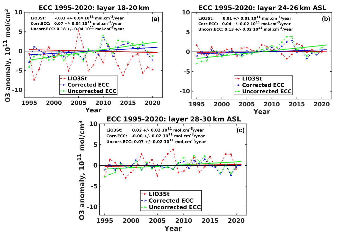
Figure 12Interannual variation of deseasonalized O3 concentrations in for the uncorrected ECC (green), homogenized ECC (blue) and LiO3St (red) for 3 altitude ranges in the stratosphere: 18–20 km (a), 24–26 km (b) and 28–30 km (c). The regression lines through all the O3 anomalies between 1995 and 2020, O3 trends (in ) and their uncertainties with a 95 % confidence are shown in each panel.
Table 2Stratospheric trends and their confidence limit for lidar, uncorrected ECC and homogenized ECC.

The 30-year ozone dataset from weekly ECC ozone soundings has been homogenized according to the recommendations of Smit et al. (2012). The major changes are related to the change of ECC manufacturer in 1997 (SPC-SST 1 % to EnSci-SST 1 %), the background current and internal sonde temperature corrections. The assessment of the OHP ECC homogenization benefit has been carried out using comparisons with ground-based instruments located at the same station (lidar, surface measurements) and satellite overpass observations (MLS in the stratosphere and GOME/OMI/OMPS for the total ozone column, TOC). The major findings are the following:
-
The 3–4 ppb positive bias of the ECC in the troposphere due to the use of uncorrected EnSci-SST 1 % and a pressure-dependent Ib is corrected with the homogenization, leading to a better agreement between the LiO3Tr lidar and ECC data in the mid-troposphere.
-
The ECC trends of the seasonally adjusted ozone concentrations are significantly improved both in the troposphere and the stratosphere when the ECC concentrations are homogenized, as shown by the ECC/lidar or ECC/TEI trend comparisons.
-
The negative trend of the normalization factor (NT) calculated using the OHP Dobson and SAOZ total column disappears thanks to the homogenization of the ECC. There is, however, a remaining −3.7 % negative bias which is likely related to an underestimate of the ECC concentrations in the stratosphere above 50 hPa as shown by comparison with the OHP LiO3St lidar. The reason for this bias is still unclear and must be better understood.
-
Differences between TOC measured by ECC and by GOME or OMI/OMPS switch from 2±2 % for uncorrected ECC to % for homogenized ECC. The negative bias is then smaller than the −3.7 % obtained with the OHP TOC measurements, even though the time evolution is consistent with the NT time distribution.
-
Direct comparisons of homogenized and uncorrected ECC concentrations in the stratosphere between 18 and 26 km show limited changes using a subset of 40 d, with LiO3St and ECC measurement time difference less than 6 h. The mean differences between 2005 and 2021 ECC and MLS or LIO3St ozone observations using a less restrictive time coincidence of <12 h are either slightly positive (+2 %) for MLS or slightly negative (−2 %) for LiO3St, meaning that the homogenization is a good compromise for intercomparability of ECC with other stratospheric O3 measurements below 26 km.
-
The comparisons with both lidar and satellite observations suggest that homogenization increases the negative bias of the ECC to values lower than −6 % above 26 km.
While the objective of this paper is to discuss the impact of homogenization on the OHP dataset using lidar and satellite measurements, it is worth checking how such corrections have improved data quality at other sites. The impact of the homogenization is dependent on the site, because different homogenization steps have to be applied at different stations. In general, the additional corrections for the pump temperature will give higher ozone partial pressure amounts in the stratosphere. On the other hand, applying a constant background current subtraction instead of a pressure-dependent background current and applying the transfer functions from EnSci-SST 1 % will lead to lower ozone partial pressure values above 10 km. Witte et al. (2017) performed an extensive analysis of seven Southern Hemisphere Additional Ozonesondes (SHADOZ) network stations in the tropics, showing that the mean differences between ECC and MLS are reduced from % to % at 40 hPa (22 km) and from % to % at 17 hPa (28 km). In Europe, Van Malderen et al. (2016) observed that the O3S-DQA corrections actually give higher (+1 %) and lower (−2 %) ozone concentrations in the stratosphere with respect to standard processing for the Uccle 1997–2014 and De Bilt 1993–2014 ECC observations, respectively. This is mainly due to the fact that the pump temperature correction was a major correction for Uccle, while changing the background current correction has a major effect for De Bilt. O3S-DQA corrections reduce the relative O3 difference between Uccle and De Bilt in the lower stratosphere. The analysis of homogenized ECC at OHP using LiO3St or MLS show similar improvements in the stratosphere below 26 km. The remaining bias of −2 % to −3.7 % between homogenized ECC and other techniques measuring O3 in the stratosphere at OHP is also in the range of the remaining differences between homogenized ECC and MLS observed in the 22 to 28 km altitude range by four stations of the SHADOZ network (Witte et al., 2017).
OHP ECC data are available at https://doi.org/10.25326/293 (Ancellet, 2021). LiO3Tr data are in ohto*.anl files available at https://ftp.cpc.ncep.noaa.gov/ndacc/station/ohp/ames/lidar (last access: 27 January 2022; NOAA/NDACC, 2022b) and LiO3St data are in oho*.gol files available at https://ftp.cpc.ncep.noaa.gov/ndacc/station/ohp/ames/lidar (last access: 27 January 2022; NOAA/NDACC, 2022a). MLS/Aura Level 2 Ozone (O3) Mixing Ratio V005 data are available at https://doi.org/10.5067/Aura/MLS/DATA2516 (Schwartz et al., 2020). OMI/Aura Ozone (O3) Total Column Daily L2 data are available at https://doi.org/10.5067/Aura/OMI/DATA2025 (Bhartia, 2012). OMPS-NPP L2 NM Ozone (O3) Total Column L2 data are available at https://doi.org/10.5067/0WF4HAAZ0VHK (Jaross, 2017). GOME 2A and B data are available at http://www.eumetsat.int (last access: 27 January 2022; EUTMETSAT, 2022). Meteorological analysis data are available at ECMWF (http://www.ecmwf.int, last access: 27 January 2022; ECMWF, 2022). The OHP ECC homogenization code is available on request (Renaud Bodichon, rboipsl@ipsl.jussieu.fr).
GA, SGB and HGJS proposed the study. HGJS and RVM provided the guidelines for the homogenization of the OHP ECC data. RB wrote the homogenization software for the OHP ECC data. GA, SGB and AP provided the OHP lidar and SAOZ data. GA carried out the analysis and wrote the paper. RMS carried out the comparison of ECC and satellite data. All the authors contributed to discussion and feedback essential to the study.
At least one of the (co-)authors is a member of the editorial board of Atmospheric Measurement Techniques. The peer-review process was guided by an independent editor, and the authors also have no other competing interests to declare.
Publisher's note: Copernicus Publications remains neutral with regard to jurisdictional claims in published maps and institutional affiliations.
This article is part of the special issue “Atmospheric ozone and related species in the early 2020s: latest results and trends (ACP/AMT inter-journal SI)”. It is not associated with a conference.
The technical staff of Observatoire de Haute Provence are gratefully acknowledged for carrying out the lidar measurements and ECC ozone soundings. We acknowledge the European Centre for Medium-Range Weather Forecasts (ECMWF) for providing meteorological reanalysis for lidar data processing and dynamical tropopause altitude calculations. The authors acknowledge the NASA/GSFC AURA Validation Data Center and EUMETSAT for providing the satellite data used in this paper (MLS, GOME, OMI, OMPS).
This research has been supported by the Centre National de la Recherche Scientifique/INSU (project NDACC-France and ACTRIS).
This paper was edited by Ja-Ho Koo and reviewed by two anonymous referees.
Ancellet, G.: Tropospheric O3 profiles data using ECC ozonesonde measurements at the OHP, Aeris [data set], https://doi.org/10.25326/293, 2021. a, b
Ancellet, G. and Beekmann, M.: Evidence for changes in the ozone concentrations in the free troposphere over southern france from 1976 to 1995, Atmos. Environ., 31, 2835–2851, https://doi.org/10.1016/S1352-2310(97)00032-0, 1997. a
Ancellet, G. and Ravetta, F.: On the usefulness of an airborne lidar for O3 layer analysis in the free troposphere and the planetary boundary layer, J. Environ. Monitor., 5, 47–56, https://doi.org/10.1039/B205727A, 2003. a
Bhartia, P. K.: OMI/Aura Ozone (O3) Total Column Daily L2 Global Gridded 0.25 degree x 0.25 degree V3, Goddard Earth Sciences Data and Information Services Center (GES DISC) [data set], https://doi.org/10.5067/Aura/OMI/DATA2025, 2012. a, b
Beekmann, M., Ancellet, G., Megie, G., Smit, H., and Kley, D.: Intercomparison campaign for vertical ozone profiling in the troposphere at the Observatoire de Haute Provence, 1989: electrochemical sondes of ECC and Brewer–Mast type and a ground-based UV-DIAL lidar, J. Atmos. Chem., 19, 259–288, https://doi.org/10.1007/BF00694614, 1994. a
Chang, K.-L., Cooper, O. R., Gaudel, A., Petropavlovskikh, I., and Thouret, V.: Statistical regularization for trend detection: an integrated approach for detecting long-term trends from sparse tropospheric ozone profiles, Atmos. Chem. Phys., 20, 9915–9938, https://doi.org/10.5194/acp-20-9915-2020, 2020. a
Cohen, Y., Petetin, H., Thouret, V., Marécal, V., Josse, B., Clark, H., Sauvage, B., Fontaine, A., Athier, G., Blot, R., Boulanger, D., Cousin, J.-M., and Nédélec, P.: Climatology and long-term evolution of ozone and carbon monoxide in the upper troposphere–lower stratosphere (UTLS) at northern midlatitudes, as seen by IAGOS from 1995 to 2013, Atmos. Chem. Phys., 18, 5415–5453, https://doi.org/10.5194/acp-18-5415-2018, 2018. a
Deshler, T., Stübi, R., Schmidlin, F. J., Mercer, J. L., Smit, H. G. J., Johnson, B. J., Kivi, R., and Nardi, B.: Methods to homogenize electrochemical concentration cell (ECC) ozonesonde measurements across changes in sensing solution concentration or ozonesonde manufacturer, Atmos. Meas. Tech., 10, 2021–2043, https://doi.org/10.5194/amt-10-2021-2017, 2017. a
EUTMETSAT: GOME 2A and B, EUTMETSAT, http://www.eumetsat.int, last access: 27 January 2022. a
ECMWF: Meteorological analysis data, ECMWF, http://www.ecmwf.int, last access: 27 January 2022. a
Froidevaux, L., Jiang, Y. B., Lambert, A., Livesey, N. J., Read, W. G., Waters, J. W., Browell, E. V., Hair, J. W., Avery, M. A., McGee, T. J., Twigg, L. W., Sumnicht, G. K., Jucks, K. W., Margitan, J. J., Sen, B., Stachnik, R. A., Toon, G. C., Bernath, P. F., Boone, C. D., Walker, K. A., Filipiak, M. J., Harwood, R. S., Fuller, R. A., Manney, G. L., Schwartz, M. J., Daffer, W. H., Drouin, B. J., Cofield, R. E., Cuddy, D. T., Jarnot, R. F., Knosp, B. W., Perun, V. S., Snyder, W. V., Stek, P. C., Thurstans, R. P., and Wagner, P. A.: Validation of Aura Microwave Limb Sounder stratospheric ozone measurements, J. Geophys. Res., 113, D15S20, https://doi.org/10.1029/2007JD008771, 2008. a
Gaudel, A., Cooper, O., Ancellet, G., Barret, B., Boynard, A., Burrows, J., Clerbaux, C., Coheur, P.-F., Cuesta, J., Cuevas, E., Doniki, S., Dufour, G., Ebojie, F., Foret, G., Garcia, O., Granados Muños, M., Hannigan, J., Hase, F., Huang, G., Hassler, B., Hurtmans, D., Jaffe, D., Jones, N., Kalabokas, P., Kerridge, B., Kulawik, S., Latter, B., Leblanc, T., Le Flochmoën, E., Lin, W., Liu, J., Liu, X., Mahieu, E., McClure-Begley, A., Neu, J., Osman, M., Palm, M., Petetin, H., Petropavlovskikh, I., Querel, R., Rahpoe, N., Rozanov, A., Schultz, M., Schwab, J., Siddans, R., Smale, D., Steinbacher, M., Tanimoto, H., Tarasick, D., Thouret, V., Thompson, A., Trickl, T., Weatherhead, E., Wespes, C., Worden, H., Vigouroux, C., Xu, X., Zeng, G., and Ziemke, J.: Tropospheric Ozone Assessment Report: Present-day distribution and trends of tropospheric ozone relevant to climate and global atmospheric chemistry model evaluation, Elem. Sci. Anth., 6, 39–96, https://doi.org/10.1525/elementa.291, 2018. a
Godin-Beekmann, S., Porteneuve, J., and Garnier, A.: Systematic DIAL lidar monitoring of the stratospheric ozone vertical distribution at Observatoire de Haute-Provence (43.9∘ N, 5.71∘ E), J. Environ. Monitor., 5, 57–67, https://doi.org/10.1039/B205880D, 2002. a
Hendrick, F., Pommereau, J.-P., Goutail, F., Evans, R. D., Ionov, D., Pazmino, A., Kyrö, E., Held, G., Eriksen, P., Dorokhov, V., Gil, M., and Van Roozendael, M.: NDACC/SAOZ UV-visible total ozone measurements: improved retrieval and comparison with correlative ground-based and satellite observations, Atmos. Chem. Phys., 11, 5975–5995, https://doi.org/10.5194/acp-11-5975-2011, 2011. a, b
Jaross, G.: (2017), OMPS-NPP L2 NM Ozone (O3) Total Column swath orbital V2, Goddard Earth Sciences Data and Information Services Center (GES DISC) [data set], Greenbelt, MD, USA, https://doi.org/10.5067/0WF4HAAZ0VHK, 2017. a, b
Komhyr, W. D.: Operations Handbook–Ozone Measurements to 40 km Altitude with Model 4A Electrochemical Concentration Cell (ECC) Ozonesondes (Used with 1680 MHz Radiosondes), NOAA Technical Memorandum ERL ARL-149, Air Resources Laboratory, Silver Spring, Maryland, 49 pp., 1986. a
Leblanc, T., Sica, R. J., van Gijsel, J. A. E., Godin-Beekmann, S., Haefele, A., Trickl, T., Payen, G., and Liberti, G.: Proposed standardized definitions for vertical resolution and uncertainty in the NDACC lidar ozone and temperature algorithms – Part 2: Ozone DIAL uncertainty budget, Atmos. Meas. Tech., 9, 4051–4078, https://doi.org/10.5194/amt-9-4051-2016, 2016. a, b
Liu, G., Liu, J., Tarasick, D. W., Fioletov, V. E., Jin, J. J., Moeini, O., Liu, X., Sioris, C. E., and Osman, M.: A global tropospheric ozone climatology from trajectory-mapped ozone soundings, Atmos. Chem. Phys., 13, 10659–10675, https://doi.org/10.5194/acp-13-10659-2013, 2013. a
McPeters, R. D. and Labow, G. J.: Climatology 2011: An MLS and sonde derived ozone climatology for satellite retrieval algorithms, J. Geophys. Res., 117, D10303, https://doi.org/10.1029/2011JD017006, 2012. a, b
Nair, P. J., Godin-Beekmann, S., Pazmiño, A., Hauchecorne, A., Ancellet, G., Petropavlovskikh, I., Flynn, L. E., and Froidevaux, L.: Coherence of long-term stratospheric ozone vertical distribution time series used for the study of ozone recovery at a northern mid-latitude station, Atmos. Chem. Phys., 11, 4957–4975, https://doi.org/10.5194/acp-11-4957-2011, 2011. a, b
Nair, P. J., Godin-Beekmann, S., Kuttippurath, J., Ancellet, G., Goutail, F., Pazmiño, A., Froidevaux, L., Zawodny, J. M., Evans, R. D., Wang, H. J., Anderson, J., and Pastel, M.: Ozone trends derived from the total column and vertical profiles at a northern mid-latitude station, Atmos. Chem. Phys., 13, 10373–10384, https://doi.org/10.5194/acp-13-10373-2013, 2013. a
NOAA/NDACC: LiO3St data, NOAA/NDACC, https://ftp.cpc.ncep.noaa.gov/ndacc/station/ohp/ames/lidar/oho*.gol, last access: 27 January 2022a. a
NOAA/NDACC: LiO3Tr data, NOAA/NDACC, https://ftp.cpc.ncep.noaa.gov/ndacc/station/ohp/ames/lidar/ohto*.anl, last access: 27 January 2022b. a
Petkov, B. H., Vitale, V., Tomasi, C., Siani, A. M., Seckmeyer, G., Webb, A., Smedley, A. R. D., Rocco Casale, G., Werner, R., Lanconelli, C., Mazzola, M., Lupi, A., Busetto, M., Diémoz, H., Goutail, F., Köhler, U., Mendeva, B. T., Josefsson, W., Moore, D., López Bartolomé, M., Moret González, J. R., Mišaga, O., Dahlback, A., Tóth, Z., Varghese, S., De Backer, H., Stübi, R., and Vaníček, K.: Response of the ozone column over Europe to the 2011 Arctic ozone depletion event according to ground-based observations and assessment of the consequent variations in surface UV irradiance, Atmos. Environ., 85, 169–178, https://doi.org/10.1016/j.atmosenv.2013.12.005, 2014. a
Richards, N. A. D., Arnold, S. R., Chipperfield, M. P., Miles, G., Rap, A., Siddans, R., Monks, S. A., and Hollaway, M. J.: The Mediterranean summertime ozone maximum: global emission sensitivities and radiative impacts, Atmos. Chem. Phys., 13, 2331–2345, https://doi.org/10.5194/acp-13-2331-2013, 2013. a
Schwartz, M., Froidevaux, L., Livesey, N., and Read, W.: MLS/Aura Level 2 Ozone (O3) Mixing Ratio V005, Goddard Earth Sciences Data and Information Services Center (GES DISC) [data set], Greenbelt, MD, USA, https://doi.org/10.5067/Aura/MLS/DATA2516, 2020. a, b
Smit, H. and Thompson, A.: Ozonesonde Measurement Principles and Best Operational Practices: ASOPOS 2.0 (Assessment of Standard Operating Procedures for Ozonesondes), WMO, GAW Report No. 268, https://library.wmo.int/doc_num.php?explnum_id=10884 (last access: 9 May 2022), 2021. a, b, c, d, e, f
Smit, H., Oltmans, S., Deshler, T., Tarasick, D., Johnson, B., Schmidlin, F., Stuebi, R., and Davies, J.: SI2N/O3S-DQA activity: Guidelines for homogenization of ozone sonde data, Activity as part of SPARC-IGACO-IOC Assessment (SI2N) “Past Changes In The Vertical Distribution Of Ozone Assessment”, WCRP/SPARC Publications, http://www-das.uwyo.edu/~deshler/NDACC_O3Sondes/O3s_DQA/O3S-DQA-Guidelines%20Homogenization-V2-19November2012.pdf (last access: 9 May 2022), 2012. a, b, c
Stauffer, R. M., Morris, G. A., Thompson, A. M., Joseph, E., Coetzee, G. J. R., and Nalli, N. R.: Propagation of radiosonde pressure sensor errors to ozonesonde measurements, Atmos. Meas. Tech., 7, 65–79, https://doi.org/10.5194/amt-7-65-2014, 2014. a
Stauffer, R. M., Thompson, A. M., Kollonige, D. E., Witte, J. C., Tarasick, D. W., Davies, J., Vömel, H., Morris, G. A., Van Malderen, R., Johnson, B. J., Querel, R. R., Selkirk, H. B., Stübi, R., and Smit, H. G. J.: A Post-2013 Dropoff in Total Ozone at a Third of Global Ozonesonde Stations: Electrochemical Concentration Cell Instrument Artifacts ?, Geophys. Res. Lett., 47, e2019GL086791, https://doi.org/10.1029/2019GL086791, 2020. a, b
Szela̧g, M. E., Sofieva, V. F., Degenstein, D., Roth, C., Davis, S., and Froidevaux, L.: Seasonal stratospheric ozone trends over 2000–2018 derived from several merged data sets, Atmos. Chem. Phys., 20, 7035–7047, https://doi.org/10.5194/acp-20-7035-2020, 2020. a
Tarasick, D. W., Smit, H. G. J., Thompson, A. M., Morris, G. A., Witte, J. C., Davies, J., Nakano, T., Van Malderen, R., Stauffer, R. M., Johnson, B. J., Stübi, R., Oltmans, S. J., and Vömel, H.: Improving ECC Ozonesonde Data Quality: Assessment of Current Methods and Outstanding Issues, Earth Space Sci., 8, e2019EA000914, https://doi.org/10.1029/2019EA000914, 2021. a, b
Thompson, A. M., Stauffer, R. M., Wargan, K., Witte, J. C., Kollonige, D. E., and Ziemke, J. R.: Regional and Seasonal Trends in Tropical Ozone From SHADOZ Profiles: Reference for Models and Satellite Products, J. Geophys. Res.-Atmos., 126, e2021JD034691, https://doi.org/10.1029/2021JD034691, 2021. a, b
Thornton, D. C. and Niazy, N.: Effects of solution mass transport on the ECC ozonesonde background current, Geophys. Res. Lett., 10, 97–100, https://doi.org/10.1029/GL010i001p00097, 1983. a
Van Malderen, R., Allaart, M. A. F., De Backer, H., Smit, H. G. J., and De Muer, D.: On instrumental errors and related correction strategies of ozonesondes: possible effect on calculated ozone trends for the nearby sites Uccle and De Bilt, Atmos. Meas. Tech., 9, 3793–3816, https://doi.org/10.5194/amt-9-3793-2016, 2016. a, b
Van Roozendael, M., Peeters, P., Roscoe, H. K., De Backer, H., Jones, A. E., Bartlett, L., Vaughan, G., Goutail, F., Pommereau, J.-P., Kyro, E., Wahlstrom, C., Braathen, G., and Simon, P. C.: Validation of Ground-Based Visible Measurements of Total Ozone by Comparison with Dobson and Brewer Spectrophotometers, J. Atmos. Chem., 29, 55–83, https://doi.org/10.1023/A:1005815902581, 1998. a
Vömel, H. and Diaz, K.: Ozone sonde cell current measurements and implications for observations of near-zero ozone concentrations in the tropical upper troposphere, Atmos. Meas. Tech., 3, 495–505, https://doi.org/10.5194/amt-3-495-2010, 2010. a
Witte, J. C., Thompson, A. M., Smit, H. G. J., Fujiwara, M., Posny, F., Coetzee, G. J. R., Northam, E. T., Johnson, B. J., Sterling, C. W., Mohamad, M., Ogino, S.-Y., Jordan, A., and da Silva, F. R.: First reprocessing of Southern Hemisphere ADditional OZonesondes (SHADOZ) profile records (1998–2015): 1. Methodology and evaluation, J. Geophys. Res.-Atmos., 122, 6611–6636, https://doi.org/10.1002/2016JD026403, 2017. a, b
Witte, J. C., Thompson, A. M., Smit, H. G. J., Vömel, H., Posny, F., and Stübi, R.: First Reprocessing of Southern Hemisphere ADditional OZonesondes Profile Records: 3. Uncertainty in Ozone Profile and Total Column, J. Geophys. Res.-Atmos., 123, 3243–3268, https://doi.org/10.1002/2017JD027791, 2018. a
Zhang, J., Tian, W., Wang, Z., Xie, F., and Wang, F.: The Influence of ENSO on Northern Midlatitude Ozone during the Winter to Spring Transition, J. Climate, 28, 4774–4793, https://doi.org/10.1175/JCLI-D-14-00615.1, 2015. a
- Abstract
- Introduction
- Description of the ozonesonde homogenization
- Data and homogenization assessment
- Results and discussion
- Conclusions
- Code and data availability
- Author contributions
- Competing interests
- Disclaimer
- Special issue statement
- Acknowledgements
- Financial support
- Review statement
- References