the Creative Commons Attribution 4.0 License.
the Creative Commons Attribution 4.0 License.
 | 21 Jan 2022
Evaluating uncertainty in sensor networks for urban air pollution insights
Olalekan A. M. Popoola
Roderic L. Jones
Nicholas A. Martin
Jim Mills
Elizabeth R. Fonseca
Amy Stidworthy
Ella Forsyth
David Carruthers
Megan Dupuy-Todd
Felicia Douglas
Katie Moore
Rishabh U. Shah
Lauren E. Padilla
Ramón A. Alvarez
Ambient air pollution poses a major global public health risk. Lower-cost air quality sensors (LCSs) are increasingly being explored as a tool to understand local air pollution problems and develop effective solutions. A barrier to LCS adoption is potentially larger measurement uncertainty compared to reference measurement technology. The technical performance of various LCSs has been tested in laboratory and field environments, and a growing body of literature on uses of LCSs primarily focuses on proof-of-concept deployments. However, few studies have demonstrated the implications of LCS measurement uncertainties on a sensor network's ability to assess spatiotemporal patterns of local air pollution. Here, we present results from a 2-year deployment of 100 stationary electrochemical nitrogen dioxide (NO2) LCSs across Greater London as part of the Breathe London pilot project (BL). We evaluated sensor performance using collocations with reference instruments, estimating ∼ 35 % average uncertainty (root mean square error) in the calibrated LCSs, and identified infrequent, multi-week periods of poorer performance and high bias during summer months. We analyzed BL data to generate insights about London's air pollution, including long-term concentration trends, diurnal and day-of-week patterns, and profiles of elevated concentrations during regional pollution episodes. These findings were validated against measurements from an extensive reference network, demonstrating the BL network's ability to generate robust information about London's air pollution. In cases where the BL network did not effectively capture features that the reference network measured, ongoing collocations of representative sensors often provided evidence of irregularities in sensor performance, demonstrating how, in the absence of an extensive reference network, project-long collocations could enable characterization and mitigation of network-wide sensor uncertainties. The conclusions are restricted to the specific sensors used for this study, but the results give direction to LCS users by demonstrating the kinds of air pollution insights possible from LCS networks and provide a blueprint for future LCS projects to manage and evaluate uncertainties when collecting, analyzing, and interpreting data.
- Article
(3996 KB) - Full-text XML
-
Supplement
(2081 KB) - BibTeX
- EndNote


Ambient (outdoor) air pollution is a leading contributor to human disease and mortality around the world, causing more than 4 million premature deaths annually, with the greatest health burden in low- and middle-income countries (WHO, 2018; HEI, 2020). Within cities, the burden of air pollution is not distributed equally, with significant spatial heterogeneity in sources, concentrations, and exposures (e.g., Apte et al., 2017; Clark et al., 2014; Miller et al., 2020; Shah et al., 2020). Many of the world's most populous and polluted regions are also those with limited air quality monitoring infrastructure, restricting the potential for data-driven air quality management or public awareness campaigns (Pinder et al., 2019). Even in many high-income countries, ambient air pollution monitoring is relatively sparse (e.g., Apte et al., 2017; US GAO, 2020). Reference monitoring stations are state of the art in terms of accuracy and reliability and are required for regulatory reporting (EU, 2008). However, they are costly (∼ 104–105 USD).
Lower-cost air quality sensors (LCSs) are increasingly being explored as an alternative or supplement to reference monitors. LCSs are orders of magnitude less expensive (∼ 102–104 USD) and are therefore more suitable for dense deployments. They are commercially available from numerous manufacturers, and the market is expanding rapidly. The literature on LCSs has primarily focused on technical evaluations of sensor performance in laboratory or field settings (Castell et al., 2017; Duvall et al., 2016; Jiao et al., 2016; Karagulian et al., 2019; Kelly et al., 2017; Lewis et al., 2016; Mead et al., 2013). Comprehensive reviews of sensor technology have identified common performance issues including drifting baselines and cross-interference from other pollutants as well as sensitivity to environmental conditions such as temperature and relative humidity (WMO, 2021). The literature also presents a variety of approaches for improving the accuracy of unprocessed sensor data, including calibrations using collocations with reference instruments, in-field calibrations without collocations, and machine learning techniques, among others (Kim et al., 2018; Munir et al., 2019; Sahu et al., 2021; Spinelle et al., 2015; Zimmerman et al., 2018).
A growing body of literature on uses of LCSs primarily focuses on scientific applications and proof-of-concept deployments. Case studies have demonstrated the potential for LCS networks to provide data insights about a local air pollution environment, including characterizing spatiotemporal trends in ambient air quality (Castell et al., 2018; Caubel et al., 2019; Mead et al., 2013; Pope et al., 2018; Popoola et al., 2018) and improving air quality models through data fusion or assimilation (Bi et al., 2020; Carruthers et al., 2019; Gupta et al., 2018; Lopez-Restrepo et al., 2021). While previous LCS deployments often consider uncertainty of individual sensors relative to a reference instrument, we are unaware of network deployments where the spatiotemporal observations have been directly compared to results from a reference network.
As LCS technology becomes more ubiquitous, there is growing interest from governments and civil society to use data from LCS monitoring networks in air quality assessment and urban planning. To manage the inherent uncertainties in LCSs, guidance is needed on how users can evaluate sensor performance and decide on the most appropriate and robust uses of their data. In this work, we evaluate a sensor network's ability to characterize spatiotemporal air pollution patterns in the megacity of Greater London by using data from an LCS monitoring network deployed as part of the Breathe London pilot project (BL).
London was an ideal study area for LCS evaluation due to the city's extensive network of reference air pollution monitors as well as a range of additional tools, including a detailed emissions inventory and high-resolution modeling, all of which contribute to an advanced understanding of historical and current air pollution (GLA, 2021). Further, while air pollution has improved in recent years, in 2019 an estimated 3600 to 4100 premature deaths were attributable to anthropogenic fine particulate matter (PM2.5) and nitrogen dioxide (NO2) in London alone (Dajnak et al., 2021), and pollutant concentrations remain above UK and WHO guideline levels in many areas of the city (GLA, 2020a). In 2021, the Court of Justice of the European Union ruled that the UK has been exceeding legal limits of NO2 since 2010 and that the government failed against its legal duties to put timely mitigation plans in place (The Guardian, 2021). This work focuses on NO2 data, which were a key measurand of the project based on the local regulatory priorities.
We first evaluated the performance of a subset of NO2 sensors that were collocated with reference instruments. The uncertainties determined from these evaluations were then considered in the context of specific analysis applications, or “use cases”, of LCS data, including long-term concentration trends, temporal concentration patterns (i.e., diurnal and day-of-week), and quantification of regional episodes of elevated air pollution. LCS network results were compared to results from an extensive network of London reference monitors, demonstrating the extent to which the BL network produced accurate spatiotemporal insights about air pollution and illuminating how sensor uncertainties identified during collocations affected the network's ability to characterize local air pollution.
While the BL LCS results show many areas of agreement with reference network data, with some areas of discrepancy, the comparisons are only representative of a selected sensor technology (electrochemical NO2 sensors of a specific vintage from a specific supplier) deployed in a specific environment type; care should be taken in extrapolating results to other sensors and environments (i.e., differing pollution levels and weather conditions). Nevertheless, the methods and lessons presented here can aid the design and operation of future LCS deployments by providing a blueprint for users to quantify and manage uncertainty in their own LCS datasets and explicitly consider the implications when investigating locally relevant air pollution questions.
2.1 Monitoring devices
The BL NO2 dataset includes data from 100 AQMesh units (Environmental Instruments Ltd., Firmware V 3.24), commercially available devices which have been previously tested and utilized by researchers and air quality managers (Fig. 1b) (AQMesh, 2021; AQ-SPEC, 2015; Castell et al., 2017). A detailed description of the AQMesh units can be found elsewhere (e.g., Castell et al., 2017). AQMesh measurements of nitrogen dioxide (NO2), the focus of this paper, relied on an Alphasense Ltd. O3-filtered electrochemical sensor. The AQMesh devices in BL also measured nitric oxide (NO), particulates (PM2.5 and PM10), and carbon dioxide (CO2), and 10 devices additionally measured ozone (O3).
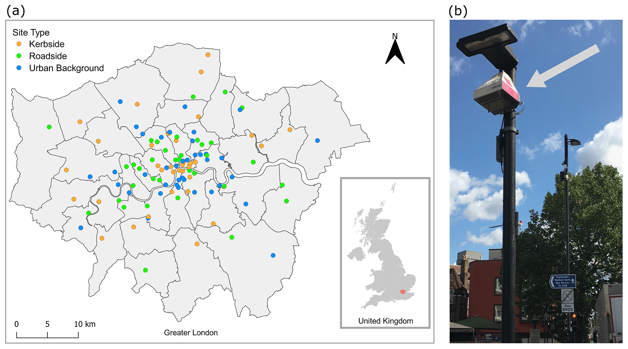
Figure 1(a) BL network locations across Greater London. (b) Picture of BL AQMesh unit (indicated by arrow) installed at Kew Road, Richmond.
2.2 Network design and deployment
We deployed AQMesh units across Greater London (Fig. 1) in areas identified in consultation with the Greater London Authority (GLA), though final locations depended on obtaining permissions from site owners. We sought locations across a range of traffic levels and at varying distances from major roads and intersections, parks, residential areas, high-traffic streets, and other commercial areas. In addition, we included monitoring at sensitive receptors, including some primary schools and medical facilities.
Each BL location was classified by site type (kerbside, roadside, or urban background) based on the local characteristics in accordance with GLA guidance for London air quality monitoring (GLA, 2018). Kerbside locations were usually within 1 m of a road and were expected to have high pollutant concentrations where traffic was the dominant source. Roadside locations were also situated near roads (usually <5 m) but were expected to be more representative of pedestrian exposure. Urban background locations were mostly sited within school yards away from dominant emissions sources such as busy roads. BL AQMesh devices were often installed marginally higher (∼ 3–4 m) than London reference monitors (∼ 2 m) to avoid physical tampering. Some monitors that were within 1 m of the road were still classified as urban background or roadside based on judgment of local features, including device height, positioning, and proximity to sources. While prevailing guidance recommends devices be placed away from structures, with 270∘ unobstructed flow, this goal was not achieved at many sites where the only option for installation and power supply was on a building façade (EU, 2008). Thus, classifications are informative but somewhat imperfect.
Of the 112 AQMesh locations in the NO2 dataset (number exceeds 100 because some sensors were relocated during the project), 36 sites were classified as kerbside, 36 as roadside, and 40 as urban background. The locations and site types are shown in Fig. 1a.
2.3 Data collection, processing, and QA/QC
We evaluated AQMesh measurements of NO2 collected during the Breathe London pilot project from September 2018 through November 2020 (Breathe London, 2021a). The devices were set to take a measurement every 10 s and delivered averaged readings every minute (i.e., an average of six readings). These 1 min data were transferred using a built-in GPRS modem to the manufacturer's (Environmental Instruments Ltd.) server in near real time, where they were processed by the manufacturer using proprietary algorithms based on their factory testing, and are termed here as prescaled data. Individual data points were accompanied by flags regarding sensor status. Data were then ingested into a data platform hosted by ACOEM Air Monitors Ltd., who also managed the monitor deployment, maintenance, and manual QA/QC process (Breathe London, 2020). Cambridge Environmental Research Consultants (CERC) applied a sensor-specific calibration gain and offset (see Sect. 2.3.1) to each device's 1 min prescaled data to produce a calibrated dataset. CERC then filtered data for valid flags and high and low limits that screened out physically unrealistic concentration measurements and averaged measurements to hourly time resolution using an 85 % data capture threshold per hour. Manual inspection of sensor data was performed weekly to identify anomalous measurements. If a sensor malfunction was identified through QA/QC protocols, ACOEM Air Monitors Ltd. technicians intervened to mitigate the issue, usually through replacement of faulty sensors.
2.3.1 Sensor calibration
NO2 sensors in the field (termed “candidate sensors” here) were calibrated using one of three methods: reference site collocation, transfer standard collocation, or remote network calibration method. For reference site collocations, a candidate AQMesh unit was installed alongside a reference monitor from the London Air Quality Network (LAQN) or UK Automatic Urban and Rural Network (AURN) (Fig. S1 shows a picture of an example reference site collocation). Transfer standard collocations relied on nine AQMesh devices that were periodically (every 2–4 months) collocated and calibrated against reference monitors; these calibrated AQMesh units were then used as transfer standards and were collocated with so-called candidate AQMesh units in the field to determine the latter's calibration parameters. The duration of typical calibration collocations was 7–14 d (for both reference and transfer standard methods), though long-term collocations were also conducted for further performance evaluation purposes. Calibration gain and offset parameters were obtained by performing a linear regression on the hourly averaged collocation time series after excluding the 1st and 99th percentile of hours during the collocation based on the ratio of reference candidate values. Calibration parameters were deemed valid and applied to the candidate sensor if the scaled collocation time series met statistical criteria of normalized root mean square error (nRMSE) <50 % (Eq. 3) and R2>0.7 (Eq. 4), which ensured that sensor performance was sufficient to calculate robust calibration parameters and effectively excluded periods where the NO2 variability was too low to provide a meaningful test of sensor gain and offset.
The remote network calibration method is a novel approach, developed and applied by the University of Cambridge project team, that remotely derives unit-by-unit calibration parameters for the entire sensor network in lieu of physical collocations. The algorithm uses a spatial scale separation methodology described in previous work (Heimann et al., 2015; Popoola et al., 2018) to calibrate sensors in relation to each other when pollution levels are consistent across the network and obtains traceability (connection to reference standard with known uncertainties) from a single calibrated reference monitor (Popoola et al., 2022; Popoola and Jones, 2020). For BL, a single (site-dependent) calibration was performed using the period May–December 2019 and applied to the entire dataset. This paper does not intend to evaluate the network calibration method compared to other approaches. The method and its performance will be addressed in more detail in a separate study (Popoola et al., 2022). However, we describe the method here because it was used to scale a subset of BL sensors which had no physical (reference or transfer) calibration available, and we include data from this subset of sensors to maximize the number of sensor locations in our analysis and comparisons to the reference network.
When multiple valid calibration options were available for a specific AQMesh sensor in the network, a decision tree was used which prioritized (i) reference site collocation (n=11), (ii) transfer standard collocation (n=73), and (iii) network calibration (n=38); the total number of calibrations applied exceeded the number of devices because failed sensors were replaced and re-calibrated.
2.3.2 Ozone cross-interference correction
A long-term upward drift in BL NO2 sensor measurements was observed (Fig. S2), which we hypothesized to be caused by an ozone cross-interference. A correction was applied to the hourly NO2 dataset that subtracted a fraction of the derived site-specific O3 concentration from the scaled NO2 readings. Site-specific O3 was deduced using upwind background reference O3 measurements; under low-NOx conditions (<10 ppb) the site-specific O3 was assumed to be the upwind background O3 concentration; otherwise it was assumed to be the difference between background O3 and the site-specific NO concentration. Because the effect appeared to increase as a sensor aged, the cross-sensitivity correction for ozone was assumed to start at 0 % upon initial sensor deployment and exponentially increase to a maximum of +18 % of estimated site-specific ozone concentrations 6 months later. Figure S2 illustrates the effect of the correction on BL network mean NO2 concentrations throughout the campaign. Figures S3 and S4 show evidence supporting the ozone cross-interference hypothesis and an evaluation of the correction method for an individual sensor. Note that due to a complex set of factors including the combination of factory (AQMesh) and field calibration methods, we could not exclude other possible causes of observed irregularities in sensor measurements. Except for the short-term collocation analysis results (Fig. 2), the results presented throughout this paper use the scaled hourly average ozone-corrected dataset.
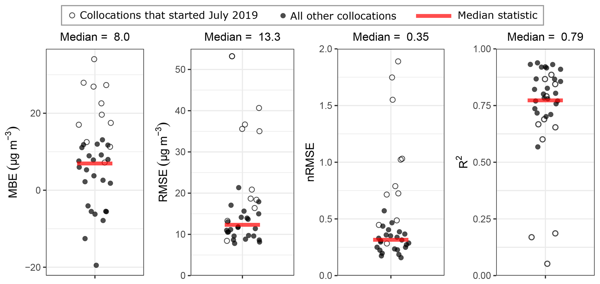
Figure 2Performance of calibrated sensors during short-term (typically 7–14 d) collocations with reference instruments. Unfilled circles are collocations that started in July 2019 during periods of elevated temperatures. Statistics calculated from hourly measurements (Eqs. 1–4).
Detailed documentation of the static network QA/QC procedures is available in the project QA/QC manual in the Breathe London Technical Report (Breathe London, 2020).
2.4 Reference and meteorological data
Hourly NO2 and O3 concentration data were downloaded for 105 reference monitors within Greater London that were classified as kerbside (n=12), roadside (n=62), or urban background (n=31) using the R openair package (Carslaw and Ropkins, 2012). These monitors, which we refer to collectively as the “reference” network, include sites from multiple overlapping UK networks including the London Air Quality Network (LAQN), Air Quality England (AQE) network, and Automatic Urban and Rural Network (AURN). At the time of download (9 June 2021) reference data were fully ratified for 69 sites. At 36 sites, some 2020 data were categorized as provisional and are thus subject to change during the ratification process. Hourly ambient air temperature observations at London Heathrow Airport, located within the Greater London study region and ∼ 25 km west of Central London, were accessed from the National Oceanic and Atmospheric Administration (NOAA) Integrated Surface Database (ISD) via the R worldmet package (NOAA, 2021; Carslaw, 2020).
2.5 Sensor performance statistics
The reference site collocations described in Sect. 2.3.1 were also used to evaluate sensor performance. A total of 98 collocations were performed between a lower-cost (LC) sensor and a reference monitor, including 10 sensors that were collocated more than once and 2 sensors that were collocated for long-term periods of >80 weeks. The statistics in Eq. (1)–(4) were used to evaluate sensor performance during reference site collocations (a representative example of collocation results is shown in Fig. S5). The following statistics were calculated from hourly time series data for each individual collocation of n h duration:
where Sen represents the BL sensor measurement, and Ref represents the observed reference measurement.
2.6 ADMS-Urban modeling data
The ADMS-Urban air pollution dispersion model was used to simulate 2019 hourly NO2 concentrations at BL and reference network monitoring locations in order to estimate the expected difference in NO2 pollution levels between the two networks (McHugh et al., 1997). The model used traffic flows and speeds and 1 km gridded emissions of NO2 from the London Atmospheric Emissions Inventory (LAEI) 2013 dataset (published in 2016), interpolated to 2019 from the 2013 base year and 2020 future predictions, combined with road traffic emissions factors from the Emission Factor Toolkit (EFT) v8 for 2019 and real-world adjustment factors to calculate road source emissions. The model includes atmospheric chemistry as well as complex urban effects including street canyons and urban canopy. Individual monitoring sites were modeled as discrete receptors with the appropriate position and height. NO2 sources from outside the modeled domain were represented using hourly background concentrations at one of four rural AURN (Automatic Rural and Urban Network) stations located outside Greater London, based on which station was upwind at that hour, and hourly meteorological data were used from London Heathrow Airport. The modeling scenario (“Hotspot 2019”) includes weekday diurnal emissions patterns to represent variations in traffic flow and improvements to LAEI traffic flow. Additional details on the ADMS-Urban model and Hotspot 2019 scenario are available in the Breathe London Technical Report (CERC, 2021). To calculate the modeled difference between BL and reference network means for the year 2019 (Sect. 3.2.1), we selected all monitor hours with valid model–observation pairs (i.e., a valid modeled and observed concentration existed at that hour) for all reference and BL sites analyzed in this paper. The modeled 2019 means were calculated for each network from the pooled monitor hours.
3.1 Network performance
3.1.1 Data capture
The BL network generated nearly 1.5 million hourly calibrated NO2 measurements from 100 devices at 112 locations over the course of the 26-month pilot campaign. The number of sensor locations producing valid, calibrated data gradually increased over the first 7 months (Fig. S6). The initial delay in network data capture was caused by logistical challenges faced at the outset of the project, including obtaining permissions for monitor deployment and conducting calibrations for each sensor. By the spring of 2019 the majority of the network was operational and generated valid data for the remainder of the project, though the total number of NO2 sensors producing valid data fluctuated due to redaction of flagged data and the downtime of sensors that failed during the project before replacement and re-calibration were performed. In total, 35 NO2 sensors were replaced due to failure, with most failures occurring during the winter. Additional considerations and lessons learned for stationary sensor network setup and maintenance are discussed in the Breathe London Blueprint (Breathe London, 2021b).
3.1.2 Measurement uncertainty of calibrated sensors
Figures 2 and 3 present measurement uncertainty statistics for calibrated BL LCSs based on short-term (typically 7–14 d) and long-term (>80 weeks) reference collocations. Both analyses quantify uncertainty of sensor measurements that were calibrated based on results of a prior reference site collocation (Sect. 2.3.1). These results allow us to evaluate the effectiveness of the project's QA/QC procedures (including calibration) since each repeat collocation serves as an independent test of the project-long uncertainties in sensors that were calibrated during a discrete time period.
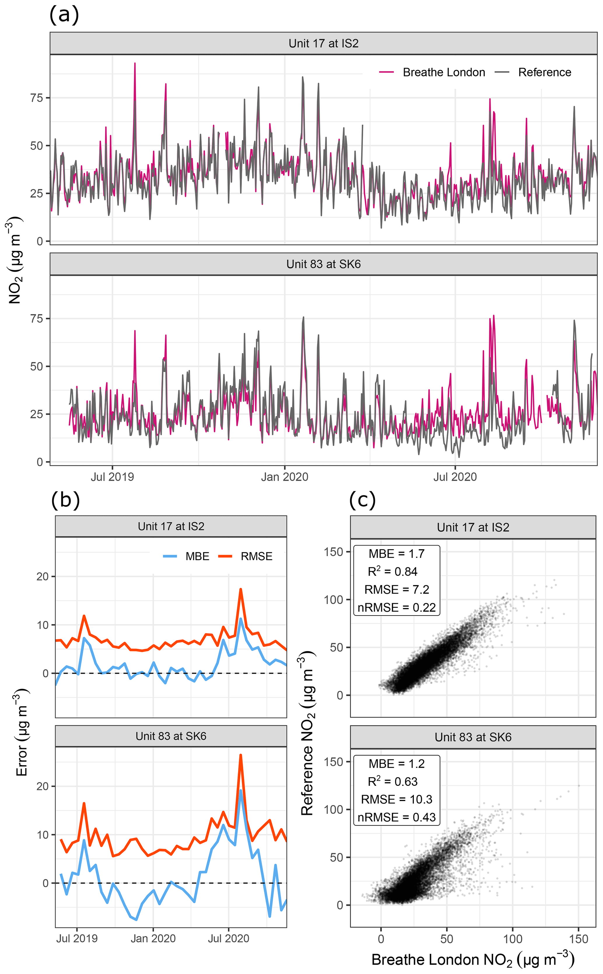
Figure 3Performance of two calibrated sensors during long-term reference collocations. Sensors were calibrated using linear regression against the reference instrument during a 2-week collocation directly preceding the evaluation period (calibration period not shown). (a) Daily mean NO2 concentration time series comparison of BL sensor and reference monitor measurements. (b) MBE (Eq. 1) and RMSE (Eq. 2) statistics of hourly BL sensor measurements compared to reference measurements during 14 d periods. (c) Scatterplot and statistics (Eqs. 1–4) comparing hourly BL sensor (x axis) and reference monitor (y axis) measurements for entire evaluation period.
Figure 2 shows evaluation results for 10 calibrated sensors that were collocated for subsequent short-term periods (typically 7–14 d) that began 1–84 weeks after an initial reference site calibration period. These subsequent collocation periods (n=35) were used to estimate calibrated sensor uncertainty compared to reference measurements (e.g., unit 99 was calibrated based on the first reference site collocation in October 2018; uncertainty statistics in Fig. 2 were calculated from the second and third reference collocations, which occurred in April and July of 2019).
A median R2 of 0.79 indicates that calibrated sensors effectively captured changes in NO2 concentrations that were measured by reference instruments. The median MBE was 8.0 µg m−3 (23 % of mean concentration) with a range of −19 to 34 µg m−3 (−37 % to 121 % of mean concentration), and the median normalized RMSE was 35 % (range of 16 % to 189 %). The large range of biases exhibited by individual sensors and the systematically high median bias of the collocated sensors reveal variability in the consistency of sensor response over time (and under different meteorological conditions) and serve to assess the robustness of initial sensor calibrations when applied to a longer time series. However, we note that uncertainty statistics in Fig. 2 are calculated from sensor data that were not corrected using the ozone cross-interference correction (Sect. 2.3.2) and thus represent an upper bound of the BL network uncertainty.
The Fig. 2 results and summary statistics are affected by a group of outlier collocations (unfilled circles in Fig. 2) that started in July 2019, during which most sensors exhibited higher measurement error and poorer correlation to reference measurements. The eight collocations with the highest normalized RMSE (>70 %) all occurred during July 2019 (Fig. S7). Additionally, seven of these July 2019 collocations had R2 values below 0.7, meaning they would have failed the statistical screening criteria used for determining valid collocation calibrations (Sect. 2.3.1). During this month, we observed high-biased sensor measurements when local air temperatures were above 20–25 ∘C, which we discuss further below. With the July 2019 collocations (n=11) excluded, the median nRMSE and MBE of the remaining collocations (n=24) improve to 30 % and 4.5 µg m−3, respectively, and the median R2 increases slightly to 0.81.
Figure 3 presents the collocation time series and monthly error statistics between calibrated BL sensor and reference monitor measurements during two long-term (>18 month) collocations, where the sensor measurements are calibrated based on the collocation results during the 2-week period directly preceding the extended evaluation period. While the aggregate MBE of both collocations is small (<2 µg m−3), BL sensors exhibit biases that vary seasonally relative to reference measurements; MBE of sensors during 14 d periods (Fig. 3b) ranges from −3 to +11 µg m−3 for unit 17 (−8 % to +34 % of the 14 d mean concentration) and from −8 to +19 µg m−3 for unit 83 (−20 % to +91 % of the 14 d mean concentration). The drifting sensor response follows the same seasonal pattern for both long-term collocations, with the highest bias occurring during summer months and peaking during August 2020. Variations in RMSE error are largely driven by sensor bias; nRMSE is highest during summer months, corresponding to peak BL sensor bias. Figure S8 further illustrates the occurrence of high-biased BL sensor measurements during hours when the local air temperature exceeded 20–25 ∘C. While the results presented above quantify uncertainty of sensors calibrated using reference collocations, the data use cases in the following sections also include sensor data calibrated using two additional approaches when sensors could not be collocated at reference sites, as described in the “Methods” section (Sect. 2.3.1): transfer standard calibration and network calibration method. The transfer standard method is more difficult to validate because collocations occur at BL sites in the field instead of at reference sites. The uncertainty of this method is expected to be marginally higher than the direct reference site collocations in Fig. 2 due to the additional step where the calibration is transferred between BL AQMesh units. A high level of precision and consistency in response across BL NO2 sensors (R2=0.94, nRMSE = 0.1; Fig. S9) gives confidence that calibrations would transfer effectively between units. Preliminary evaluations have shown that the estimated uncertainty of BL sensor measurements scaled with the network calibration method is broadly similar to the uncertainty of reference collocation-calibrated sensors (Popoola et al., 2022; Popoola and Jones, 2020). The results in Figs. 2 and 3 demonstrate that the long-term measurement uncertainty of sensors calibrated during a brief, discrete period is influenced by the changes in sensor response during different seasons and environmental conditions. Enhanced QA/QC such as calibration on a near-continuous basis or seasonal bias corrections such as the one shown in Fig. S10 (see Sect. 3.2.1) could minimize variations in measurement uncertainty due to sensor performance.
For a long-term measurement campaign using sensors, evaluation against reference measurements should be performed throughout the course of the project. The evaluation results above point to the ability of BL sensors to accurately reproduce changes in NO2 concentrations captured by the reference monitors (high R2 values) with average uncertainty (nRMSE) of ∼ 35 %. However, our results also show that seasonal biases due to time-varying effects of environmental interferences can lead to larger uncertainties (>100 % nRMSE) during periods when local air temperatures reached above 20–25 ∘C. This characterization of sensor uncertainties can inform how results from the BL LC sensor network are interpreted, ensuring derived insights are robust (e.g., differentiating between high-biased sensor artifacts and elevated NO2 concentrations).
We next present a series of analytical use cases to evaluate the applicability of BL NO2 LCS network results for deriving insights about the local air pollution environment. Results from each use case using BL data are compared against results generated from reference network data. In addition, the collocation sensor evaluations presented above are used to assess BL network uncertainty and interpret differences between BL and reference network results.
3.2 Use case validation
3.2.1 Regional pollution load and time trends
We first examine the ability of the BL sensor network to characterize trends in the regional (Greater London) pollution load by comparing monthly mean NO2 concentrations of the BL network with the reference network results (Fig. 4). We compare monthly values here to assess the sensor network's ability to reproduce long-term patterns observed by the reference network on timescales that would be sensitive to effects of seasonal variations in pollutant concentrations or sensor performance as well as long-term ambient pollution changes resulting from major interventions. We note two major events during the measurement campaign which are expected to impact NO2 concentrations: (i) introduction of the Ultra Low Emission Zone (ULEZ), which became effective on 8 April 2019, imposed tolls to discourage entry of older, higher-emitting vehicles into Central London, with increasing fractions of compliant vehicles and fewer vehicles overall observed in the zone through calendar year 2019 (GLA, 2020b), and (ii) Covid-19 pandemic restrictions beginning March 2020, including social distancing measures and stay-at-home orders, disrupted activity patterns throughout Greater London.
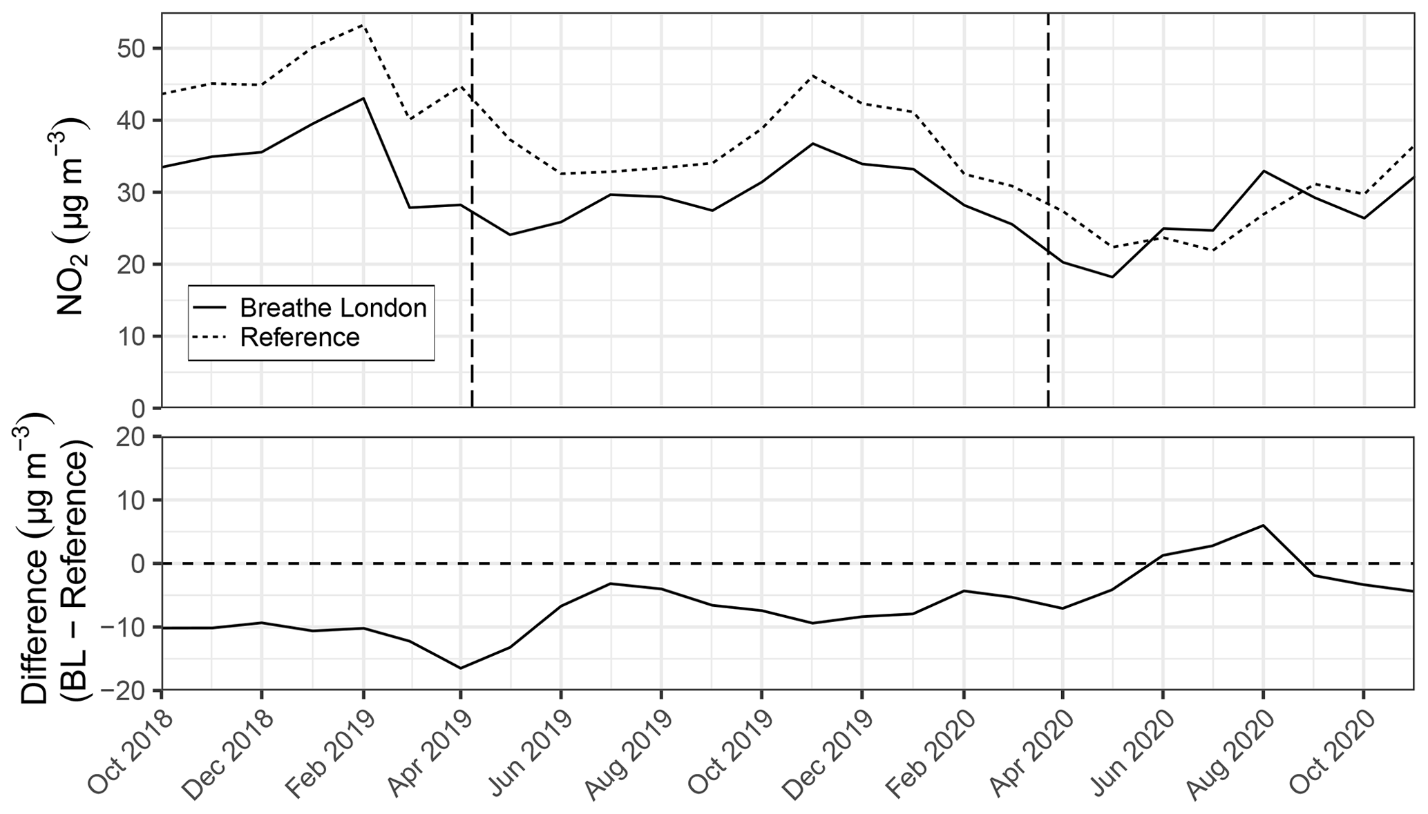
Figure 4Comparison of monthly mean NO2 concentrations for the BL (n=100) and London reference (n=105) networks. Bottom panel shows difference between networks. Vertical lines denote Ultra Low Emission Zone (ULEZ) start date (8 April 2019) and the start of the first Covid-19 lockdowns (23 March 2020).
The BL network tracked the reference network trend while exhibiting lower mean concentrations for most of the campaign (on average 7 µg m−3 lower throughout campaign; 9 µg m−3 during 2019). We attribute this partially to differences in location, site types, and sampling points (height, distance to road, road traffic volume, etc.) between the networks, and this is confirmed through comparisons of measured and modeled concentrations using the ADMS-Urban air pollution dispersion model (described in Sect. 2.6). Modeled network mean NO2 concentrations for 2019 at reference network monitoring site receptors were 5 µg m−3 higher (∼ 15 %) than the modeled mean concentrations at BL receptor locations. Because the model only predicts 55 % of the difference between the two networks, we examined the model–network comparisons more closely. The model exhibits little systematic bias at reference sites (<1 µg m−3; see Fig. S11). By contrast, the mean of modeled concentrations was higher than that observed at the BL sites by 6 µg m−3, with the difference driven by BL sites with the lowest observed concentrations (Fig. S11). We note that 16 BL sites exhibited lower concentrations than the 20 µg m−3 minimum observed by the reference network, so we cannot rule out the possibility of low sensor bias in a portion of the BL network. In sum, we are unable to fully resolve the cause of the systematic difference between modeled and observed BL concentrations, although it may have contributions from uncertainty in sensor network measurements (and underlying QA/QC) and model uncertainty.
Both networks show a downward year-on-year trend in NO2 concentrations and seasonal variability with peak concentrations in the winter. However, BL NO2 means exhibit local maxima in July and August, when reference network measurements are lowest. This effect is the most pronounced in summer 2020, which is the only time when the BL network average exceeds that of the reference network. This bias of the BL network compared to reference network trends during summer months is likely due in part to a systematic high bias in the BL network's NO2 sensors coinciding with local air temperatures above 20–25 ∘C, an effect which was evident during collocations with reference monitors (Figs. 3, S7, and S8). However, spatially varying NO2 pollution trends (e.g., Covid-19 restrictions having a larger impact on emissions at specific monitoring sites or city neighborhoods) may have also affected the two networks differently and contributed to the converging network means towards the end of the BL campaign.
The long-term collocations (Sect. 3.1.2) were used to quantify seasonal changes in sensor bias and could serve as a basis for an empirical correction to the Fig. 4 BL network time series to improve the accuracy of the LCS results. This correction relies on the performance results being consistent across the network; the high precision between AQMesh units in our transfer standard collocations (median R2=0.94; Fig. S9) supports this assumption for the BL project. In Fig. S10 we show the Fig. 4 BL time series with a monthly bias correction based on the long-term collocations that would largely mitigate the seasonal irregularities in the BL time series compared to the reference network.
3.2.2 Temporal pollution patterns
We next compare the recurring temporal patterns in NO2 concentrations measured by the BL and reference networks (Fig. 5).
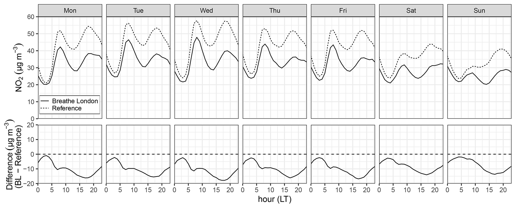
Figure 5Network mean diurnal and day-of-week NO2 concentration patterns in Greater London, as measured by the BL (n=99) and reference (n=105) networks during the pre-Covid-19 period of the BL project (1 October 2018 through 29 February 2020). Bottom panel shows difference between networks.
The BL network captures diurnal and day-of-week patterns with three key differences from the reference network. First, BL network mean concentrations are ∼ 10 µg m−3 (23 %) lower than the reference network result. Most of this difference was predicted in the modeling exercise discussed in Sect. 3.2.1, with additional contribution from uncertainty in sensor measurements. Second, BL network mean concentrations show a reduced diurnal range compared to the regulatory network (i.e., though daytime average BL concentrations are lower, nighttime values are similar to the reference network). This behavior may be due to previously discussed differences in site characteristics (e.g., higher sensor placement and lower traffic volume at near-road sites) yielding reduced heterogeneity in site types across the BL network, which as a whole appears to be measuring diurnal pollution patterns that are more in line with urban background reference sites (Fig. 6). A similar effect is observed in a comparison of near-road (kerbside and roadside) and urban background reference sites, where the concentration difference was smallest during late-night/early-morning hours (Fig. S12). A third key difference in diurnal day-of-week concentration patterns is the magnitude of the evening peak, which is consistently lower than the morning peak in the BL network. On Wednesdays, for example, the reference network evening peak reached 57 µg m−3 at 18:00 LT, while the BL network reached 40 µg m−3 at the same time; other weekdays similarly have the largest difference in network mean concentrations during the evening rush hour peak. We have not identified a mechanism to explain this difference, which is evident, to a varying degree, throughout the year (Fig. S13).
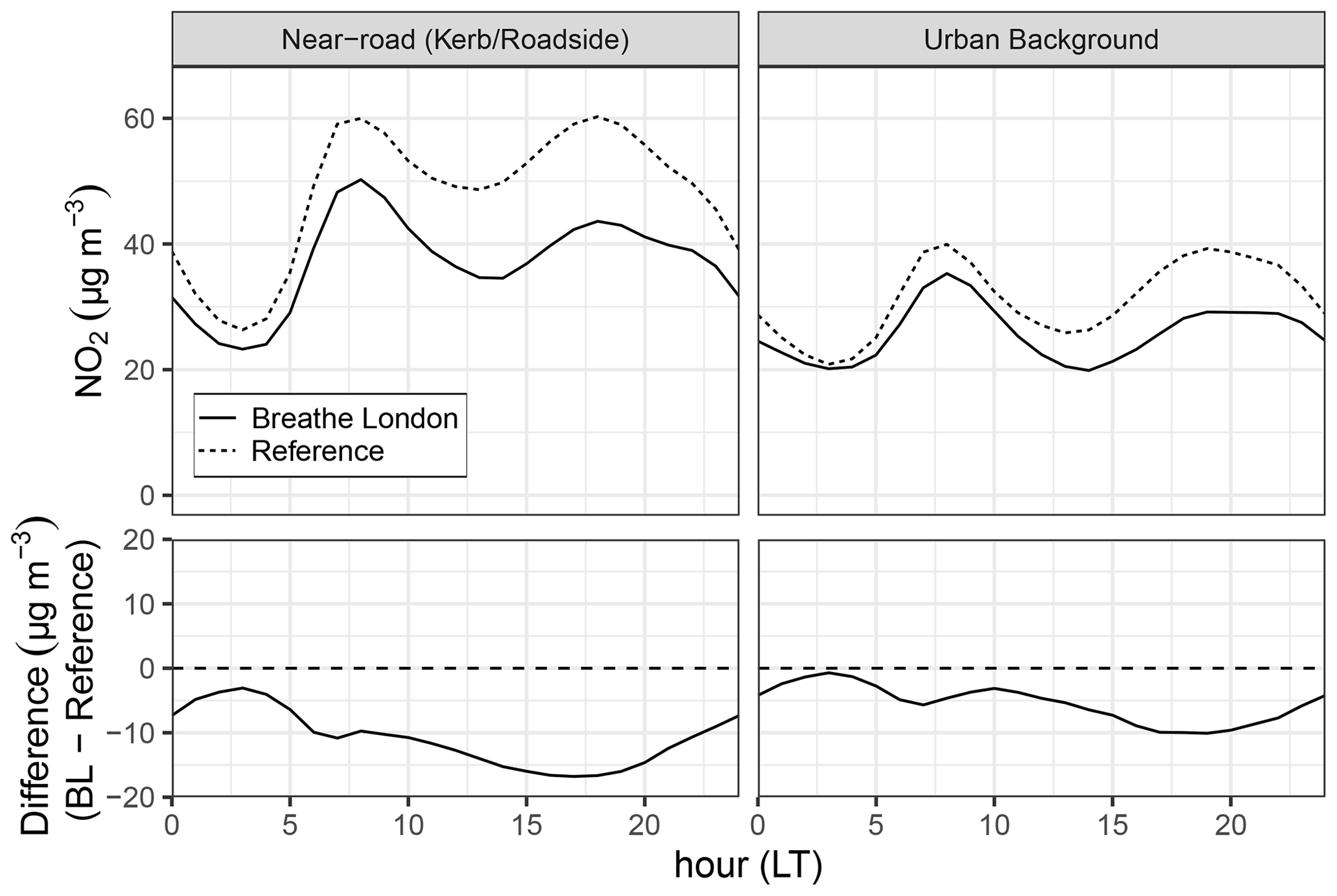
Figure 6Weekday diurnal mean NO2 concentrations in Greater London as measured by the BL (n=70 near-road, n=40 urban background; number of locations exceeds 100 because some devices were placed at multiple locations during the campaign) and reference (n=72 near-road, n=31 urban background) networks during the pre-Covid-19 period of the BL project (1 October 2018 through 29 February 2020) at two different site classification groups: near-road (left; includes sites classified as kerbside and roadside) and urban background (right). Bottom panel shows difference between networks.
The BL network was able to accurately characterize timing of peaks and troughs in diurnal variability as well as capture differences in weekday and weekend pollution levels. Uncertainties in the precise magnitudes of some features remain, with the evening peak registering relatively lower in the BL network.
3.2.3 Site type differences in diurnal pollution patterns
We next examine the ability of the BL network to detect differences in diurnal NO2 concentration patterns at different monitoring site types. Figure 6 shows the weekday diurnal averages for the BL and reference network at near-road (kerbside and roadside) sites compared to urban background sites.
In the morning, near-road concentrations peaked at 08:00–09:00 LT in both the BL and reference networks, reaching 60 µg m−3 in the reference network and 50 µg m−3 in the BL network. The time of the evening peak was also consistent between networks, occurring at 18:00–19:00 LT and reaching 60 µg m−3 in the reference network compared to a lower peak of 44 µg m−3 in the BL network at the same time. In both networks, the evening peak in concentrations occurred 1 h later (19:00–20:00 LT) at background sites than near-road sites. The greatest difference between BL and reference means at both near-road and urban background sites occurred during the evening peak in NO2 concentrations; this feature is identified in the network-wide trends in the prior section.
At this aggregate level, the lower-cost network captures similar diurnal features and effectively differentiates between pollution levels and time-of-day trends at urban background and near-road sites.
3.2.4 Hotspots and spatial heterogeneity
Here we discuss the application of BL LCS data for identifying hotspots and characterizing spatial heterogeneity in NO2 concentrations, using a case study where BL sensor measurements led to identification of an air pollution hotspot. During the first winter of the project (December 2018 through February 2019), a BL sensor deployed at Holloway Bus Garage measured mean weekday NO2 concentrations of 77 µg m−3, 89 % higher than the BL network weekday mean of 41 µg m−3 (Fig. S14). Though the concentration gradient (between Holloway Bus Garage and the BL network mean) was larger than the typical sensor uncertainties (∼ 35 % nRMSE) and occurred during winter months when large positive biases were not observed during collocation evaluations, additional steps were taken to establish confidence that the local pollution levels were accurately characterized and not sensor artifacts. Two additional BL sensors were deployed in the area, and a follow-up transfer standard collocation was performed which verified the accuracy of the deployed pod's calibration factors.
The BL monitoring at Holloway Bus Garage ultimately led to corrective action by local authorities, and this successful example demonstrates the potential value of LCSs for identifying air pollution hotspots. The case study also emphasizes the need for rigorous verification of measurements from an individual sensor. The collocation analyses quantified a wide range in the bias of BL sensors over the course of the project as well as uncertainty in the consistency of sensor performance over time (Figs. 2 and 3). Therefore, especially for concentration gradients of similar magnitude to the estimated uncertainty of the sensors, there is a need for caution when analyzing site-specific data; we established confidence in the LC sensor hotspot characterization through the deployment of additional LC sensors to verify results.
3.2.5 High-pollution episodes
Here we test the viability of the BL network to detect short- to medium-term (hours to days) episodes of elevated NO2 concentrations using a well-characterized historical air pollution event in December 2019 (LAQN, 2019). Weather conditions in Greater London resulted in the formation of a strong temperature inversion that caused a build-up of primary pollutants, including NO2, in the layer of colder air close to the ground, with pollution peaking at morning rush hour on 4 December (LAQN, 2019). Figure 7 compares the hourly mean NO2 concentrations as measured by the BL and reference networks for the week of the pollution episode.
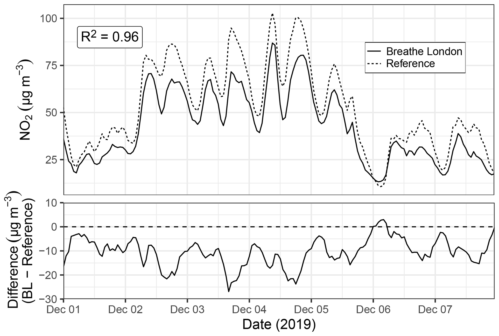
Figure 7Hourly network mean NO2 concentrations for the BL (n=85) and reference (n=105) networks during a high-pollution episode in December 2019. Bottom panel shows difference between networks.
The BL network detected a short-term regional build-up of pollution with a temporal profile that provides excellent comparability with the reference network result (R2=0.96) and corresponds to the London Air Quality Network's published report about the event. The highest peak occurred during late rush hour (09:00–10:00 LT) on the morning of 4 December, with the BL network registering a peak of 87 µg m−3 compared to 103 µg m−3 for the reference network during the same time period. Another smaller peak occurred when evening emissions were trapped on 4 December, and the event subsided when the inversion broke near midnight on 4 December. The BL lower-cost network captures the basic features of the event, although there is a low bias compared to the reference sites (nRMSE = 23 %, MBE = −11 µg m−3), partially explained by the different site types (see Sect. 3.2.1).
However, we note that the network was less effective in characterizing pollution events during periods of poorer sensor performance. In Fig. S15 we present a more cautionary case study during July 2019. We demonstrated in Sect. 3.1.2 that collocated BL sensors produced high-biased measurements during periods when local air temperatures reached above 20–25 ∘C, with worst-case nRMSE exceeding 100 % (dominated by positive bias). Figure S15 shows an instance where this effect leads to an overestimation of regional NO2 pollution levels using the BL network (for example, the BL network mean during daytime hours on 25 July 2019 is 91 µg m−3 compared to the reference network mean of 65 µg m−3, a 40 % positive bias across the network). Due to the extensive reference network in London and frequent short-term as well as ongoing long-term BL sensor collocations, we were able to identify the apparently anomalous BL sensor behavior under these environmental conditions which resulted in a systematic positive bias across the network. However, in cases with limited reference monitoring infrastructure, the BL measurements could have led to an overestimation of the magnitude of the pollution event in question. While technological and methodological solutions to address this sensor issue are viable, another project with different technologies or environmental characteristics may experience different effects, illustrating the importance of rigorous data validation and uncertainty evaluation in the context of each new application of LCS technology.
In a LCS deployment, careful evaluation of sensor performance (which may vary between projects due to, for example, specific sensor technology, firmware, local meteorology and pollution characteristics, among others) maximizes the value of the data by informing how they should be processed, analyzed, and interpreted. Robust uncertainty characterization and validation against reference instruments equips the user to take full advantage of data, including (i) developing corrections (see Fig. S10 presenting the BL network time series with a potential correction derived from collocation evaluation results), (ii) excluding measurements during conditions where sensor performance might be compromised, or (iii) ensuring analyses are appropriate based on the data quality. By contrast, we have shown that without a detailed understanding of variations in sensor performance across a campaign (see Fig. 3b illustrating temperature-related drift), biased sensor measurements at some moments during the project could have led users to overestimate pollution levels or, over longer timeframes, miss trends in concentration patterns. Our findings emphasize the importance of monitoring sensor performance for the duration of a measurement campaign as even pre- and post-campaign sensor evaluations may not have detected the seasonal changes in sensor performance that our repeat (Fig. 2) and long-term (Fig. 3) collocations allowed us to quantify. A near-real-time calibration approach may also be valuable for tracking and improving sensor performance over time by providing continuous calibrations and assessments of network performance, although a single point calibration was used here (Considine et al., 2021). Our results also demonstrate how LC sensors could be used in a city with more limited existing monitoring infrastructure than in London. The BL network generated a series of insights about air pollution in London that we compared to reference network results, and we found that the BL LCS network characterized many NO2 trends and patterns effectively, including year-over-year concentration trends, timing of diurnal peaks, weekday–weekend concentration gradients, and profiles of short- to medium-term periods of elevated pollution. We also showed how BL sensor uncertainties, which were evaluated using collocations at three London reference monitors, limited the LCS network's ability to capture precisely some features of air pollution trends, emphasizing that especially in a place without an extensive reference network, it is advisable to have at least one reliable reference instrument as a basis for ongoing LC sensor calibration and uncertainty evaluation. We also note that the use of representative reference collocations (i.e., keeping one or two units at reference sites throughout the project) to estimate network performance relies on the testable assumption that sensors are highly precise across the network.
The sensor uncertainties and data use cases that we have evaluated are specific to the sensor technology and firmware used as well as the local environmental characteristics in London. In London, environmental effects significantly impacted data quality, including frequent wintertime sensor failures and high measurement artifacts occurring when local ambient air temperatures exceeded 20–25 ∘C, indicating that sensor performance could vary in other cities with different source patterns and meteorology. Furthermore, in another environment with different air pollution levels, the same magnitude of sensor RMSE may represent a different proportion of the average concentration, reinforcing the need to evaluate sensor performance locally and consider the tolerable amount of measurement error for each application. Additionally, the current absence of a performance standard for LC sensors exposes the end user to risks in the sensor selection process, making it advisable for each implementation of LCS technology to perform its own performance evaluation. Our approach can provide a roadmap for future LCS deployments to maximize data quality and confidence in resulting insights by following robust QA/QC protocols, most notably the tracking of representative sensor performance for the duration of the project via direct traceability to reference measurements.
BL network data are available on the OpenAQ platform: https://openaq.org/#/project/28967 (Breathe London, 2022). London reference monitor data can be accessed using the R openair package (Carslaw and Ropkins, 2012). The corresponding data can also be accessed through https://www.londonair.org.uk/london/asp/datadownload.asp (LondonAir, 2022). Meteorological data are available from the NOAA Integrated Surface Database (https://www.ncdc.noaa.gov/isd; NOAA, 2021) and can be accessed via the R worldmet package (https://CRAN.R-project.org/package=worldmet; Carslaw, 2020). Collocation data are available upon request from the corresponding author.
The supplement related to this article is available online at: https://doi.org/10.5194/amt-15-321-2022-supplement.
ERF, MDT, FD, and KM managed the project, including coordinating sensor deployment and collocations. JM oversaw installation, operation, and maintenance of the sensor network. NAM hosted sensor system deployment. RLJ and OAMP developed and applied the remote network calibration method and ozone correction to the hourly NO2 dataset and were involved in data curation. AS, ERF, and DC applied the QA/QC procedure to the raw 1 min AQMesh measurements to produce a calibrated hourly dataset, curated datasets and metadata, and developed and ran model simulations. RAA, RLJ, DC, and NAM supervised research. RAA, DRP, and LEP formulated research goals for this paper. DRP prepared the manuscript, including formal analysis, visualization, and writing. All co-authors contributed to reviewing and editing.
During parts of the Breathe London pilot project, Katie Moore and Jim Mills were employed at commercial sensor providers (Clarity Movement Co. and ACOEM Air Monitors Ltd., respectively), and the University of Cambridge had a commercial arrangement with AQMesh; these relationships did not affect the work presented here. All other authors declare they have no competing interests.
Publisher’s note: Copernicus Publications remains neutral with regard to jurisdictional claims in published maps and institutional affiliations.
The Breathe London pilot project was convened by C40 Cities and the Mayor of London. The authors would like to thank the many hosts of Breathe London monitors, including local councils, schools, and residents, as well as the scientific and project advisors for their contributions. The authors are especially grateful to the local councils of Camden, Southwark, and Islington for continued access to reference monitors for collocations that were critical to this study. Thanks also to Greg Slater for his input on data visualization.
This work was supported by the Children's Investment Fund Foundation, with continued funding from the Clean Air Fund (grant numbers 1908-03995 and 341) and further funding support provided by Signe Ostby and Scott Cook (of the Valhalla Charitable Foundation) as well as funding by the Mayor of London for 10 additional AQMesh units.
This paper was edited by Dominik Brunner and reviewed by Laurent Spinelle and one anonymous referee.
Apte, J. S., Messier, K. P., Gani, S., Brauer, M., Kirchstetter, T. W., Lunden, M. M., Marshall, J. D., Portier, C. J., Vermeulen, R. C. H., and Hamburg, S. P.: High-resolution Air Pollution Mapping with Google Street View Cars: Exploiting Big Data, Environ. Sci. Technol., 51, 6999–7008, https://doi.org/10.1021/acs.est.7b00891, 2017.
AQMesh: https://www.aqmesh.com/products/aqmesh/, last access: 15 June 2021.
AQ-SPEC: AQMesh (v.4.0) – field evaluation, South Coast AQMD, available at: http://www.aqmd.gov/aq-spec/sensordetail/aqmesh-(v.4.0) (last access: 7 January 2022), Diamond Bar, CA, 2015.
Bi, J., Stowell, J., Seto, E. Y. W., English, P. B., Al-Hamdan, M. Z., Kinney, P. L., Freedman, F. R., and Liu, Y.: Contribution of low-cost sensor measurements to the prediction of PM2.5 levels: A case study in Imperial County, California, USA, Environ. Res., 180, 108810, https://doi.org/10.1016/j.envres.2019.108810, 2020.
Breathe London: AQMesh fixed sensor network data quality assurance and control procedures, available at: https://www.globalcleanair.org/files/2021/01/Breathe-London-Fixed-Sensor-Network-QAQC-Procedures.pdf (last access: 7 January 2022), 2020.
Breathe London: Breathe London archival website, available at: http://breathelondon.edf.org/, last access: 15 June 2021, 2021a.
Breathe London: The Breathe London Blueprint, available at: https://www.globalcleanair.org/files/2021/02/EDF-Europe-BreatheLondon_Blueprint-guide.pdf (last access: 7 January 2022), 2021b.
Breathe London: Breathe London Stationary, OpenAQ [data set], available at: https://openaq.org/#/project/28967, last access: 7 January 2022.
Carruthers, D., Stidworthy, A., Clarke, D., Dicks, J., Jones, R., Leslie, I., Popoola, O. A. M., and Seaton, M.: Urban emission inventory optimisation using sensor data, an urban air quality model and inversion techniques, Int. J. Environ. Pollut., 66, 252, https://doi.org/10.1504/IJEP.2019.104878, 2019.
Carslaw, D.: worldmet: Import Surface Meteorological Data from NOAA Integrated Surface Database (ISD), R package version 0.9.2, available at: https://CRAN.R-project.org/package=worldmet (last access: 7 January 2022), 2020.
Carslaw, D. and Ropkins, K.: openair – An R package for air quality data analysis, Environ. Model. Softw., 27–28, 52–61, https://doi.org/10.1016/j.envsoft.2011.09.008, 2012.
Castell, N., Dauge, F. R., Schneider, P., Vogt, M., Lerner, U., Fishbain, B., Broday, D., and Bartonova, A.: Can commercial low-cost sensor platforms contribute to air quality monitoring and exposure estimates?, Environ. Int., 99, 293–302, https://doi.org/10.1016/j.envint.2016.12.007, 2017.
Castell, N., Schneider, P., Grossberndt, S., Fredriksen, Mirjam. F., Sousa-Santos, G., Vogt, M., and Bartonova, A.: Localized real-time information on outdoor air quality at kindergartens in Oslo, Norway using low-cost sensor nodes, Environ. Res., 165, 410–419, https://doi.org/10.1016/j.envres.2017.10.019, 2018.
Caubel, J. J., Cados, T. E., Preble, C. V., and Kirchstetter, T. W.: A Distributed Network of 100 Black Carbon Sensors for 100 Days of Air Quality Monitoring in West Oakland, California, Environ. Sci. Technol., 53, 7564–7573, https://doi.org/10.1021/acs.est.9b00282, 2019.
CERC: Final report, Breathe London project, available at: https://www.globalcleanair.org/files/2021/02/BL-CERC-Final-Report.pdf (last access: 7 January 2022), 2021.
Clark, L. P., Millet, D. B., and Marshall, J. D.: National Patterns in Environmental Injustice and Inequality: Outdoor NO2 Air Pollution in the United States, PLOS ONE, 9, e94431, https://doi.org/10.1371/journal.pone.0094431, 2014.
Considine, E. M., Reid, C. E., Ogletree, M. R., and Dye, T.: Improving accuracy of air pollution exposure measurements: Statistical correction of a municipal low-cost airborne particulate matter sensor network, Environ. Pollut., 268, 115833, https://doi.org/10.1016/j.envpol.2020.115833, 2021.
Dajnak, D., Evangelopoulos, D., Kitwiroon, N., Beevers, S. D., and Walton, H.: London health burden of current air pollution and future health benefits of mayoral air quality policies, available at: http://erg.ic.ac.uk/research/home/resources/ERG_ImperialCollegeLondon_HIA_AQ_LDN_11012021.pdf (last access: 7 January 2022), 2021.
Duvall, R. M., Long, R. W., Beaver, M. R., Kronmiller, K. G., Wheeler, M. L., and Szykman, J. J.: Performance Evaluation and Community Application of Low-Cost Sensors for Ozone and Nitrogen Dioxide, Sensors, 16, 1698, https://doi.org/10.3390/s16101698, 2016.
EU: Directive 2008/50/EC of the European Parliament and of the Council of 21 May 2008 on ambient air quality and cleaner air for Europe, Off. J. Eur. Union, 152, 1–44, 2008.
Greater London Authority (GLA): Guide for monitoring air quality in London, available at: https://www.london.gov.uk/sites/default/files/air_quality_monitoring_guidance_january_2018.pdf (last access: 7 January 2022), 2018.
Greater London Authority (GLA): Air pollution monitoring data in London: 2016 to 2020, available at: https://www.london.gov.uk/sites/default/files/air_pollution_monitoring_data_in_london_2016_to_2020_feb2020.pdf (last access: 7 January 2022), 2020a.
Greater London Authority (GLA): Central London ultra low emission zone – ten month report, available at: https://www.london.gov.uk/sites/default/files/ulez_ten_month_evaluation_report_23_april_2020.pdf (last access: 7 January 2022), 2020b.
Greater London Authority (GLA): Monitoring and predicting air pollution, available at: https://www.london.gov.uk/what-we-do/environment/pollution-and-air-quality/monitoring-and-predicting-air-pollution (last access: 7 January 2022), 2021.
Gupta, P., Doraiswamy, P., Levy, R., Pikelnaya, O., Maibach, J., Feenstra, B., Polidori, A., Kiros, F., and Mills, K. C.: Impact of California Fires on Local and Regional Air Quality: The Role of a Low-Cost Sensor Network and Satellite Observations, GeoHealth, 2, 172–181, https://doi.org/10.1029/2018GH000136, 2018.
Health Effects Institute (HEI): State of Global Air 2020, Health Effects Institute, Boston, MA, 2020.
Heimann, I., Bright, V. B., McLeod, M. W., Mead, M. I., Popoola, O. A. M., Stewart, G. B., and Jones, R. L.: Source attribution of air pollution by spatial scale separation using high spatial density networks of low cost air quality sensors, Atmos. Environ., 113, 10–19, https://doi.org/10.1016/j.atmosenv.2015.04.057, 2015.
Jiao, W., Hagler, G., Williams, R., Sharpe, R., Brown, R., Garver, D., Judge, R., Caudill, M., Rickard, J., Davis, M., Weinstock, L., Zimmer-Dauphinee, S., and Buckley, K.: Community Air Sensor Network (CAIRSENSE) project: evaluation of low-cost sensor performance in a suburban environment in the southeastern United States, Atmos. Meas. Tech., 9, 5281–5292, https://doi.org/10.5194/amt-9-5281-2016, 2016.
Karagulian, F., Barbiere, M., Kotsev, A., Spinelle, L., Gerboles, M., Lagler, F., Redon, N., Crunaire, S., and Borowiak, A.: Review of the Performance of Low-Cost Sensors for Air Quality Monitoring, Atmosphere, 10, 506, https://doi.org/10.3390/atmos10090506, 2019.
Kelly, K. E., Whitaker, J., Petty, A., Widmer, C., Dybwad, A., Sleeth, D., Martin, R., and Butterfield, A.: Ambient and laboratory evaluation of a low-cost particulate matter sensor, Environ. Pollut., 221, 491–500, https://doi.org/10.1016/j.envpol.2016.12.039, 2017.
Kim, J., Shusterman, A. A., Lieschke, K. J., Newman, C., and Cohen, R. C.: The BErkeley Atmospheric CO2 Observation Network: field calibration and evaluation of low-cost air quality sensors, Atmos. Meas. Tech., 11, 1937–1946, https://doi.org/10.5194/amt-11-1937-2018, 2018.
LondonAir: Data Downloads, Imperial College London [data set], available at: https://www.londonair.org.uk/london/asp/datadownload.asp, last access: 7 January 2022.
London Air Quality Network (LAQN): LAQN Pollution Episodes, available at: https://londonair.org.uk/london/asp/publicepisodes.asp?region=0&site=&postcode=&la_id=&level=All&bulletindate=03%2F12%2F2019&MapType=Google&zoom=&lat=51.4750&lon=-0.119824&VenueCode=&bulletin=explanation&episodeID=pol3to4Dec2019&pageID=page1&cm-djitdk-djitdk= (last access 20 January 2021), 2019.
Lewis, A. C., Lee, J. D., Edwards, P. M., Shaw, M. D., Evans, M. J., Moller, S. J., Smith, K. R., Buckley, J. W., Ellis, M., Gillot, S. R., and White, A.: Evaluating the performance of low cost chemical sensors for air pollution research, Faraday Discuss., 189, 85–103, https://doi.org/10.1039/C5FD00201J, 2016.
Lopez-Restrepo, S., Yarce, A., Pinel, N., Quintero, O. L., Segers, A., and Heemink, A. W.: Urban Air Quality Modeling Using Low-Cost Sensor Network and Data Assimilation in the Aburrá Valley, Colombia, Atmosphere, 12, 91, https://doi.org/10.3390/atmos12010091, 2021.
McHugh, C. A., Carruthers, D. J., and Edmunds, H. A.: ADMS–Urban: an air quality management system for traffic, domestic and industrial pollution, Int. J. Environ. Pollut., 8, 666–674, 1997.
Mead, M. I., Popoola, O. A. M., Stewart, G. B., Landshoff, P., Calleja, M., Hayes, M., Baldovi, J. J., McLeod, M. W., Hodgson, T. F., Dicks, J., Lewis, A., Cohen, J., Baron, R., Saffell, J. R., and Jones, R. L.: The use of electrochemical sensors for monitoring urban air quality in low-cost, high-density networks, Atmos. Environ., 70, 186–203, https://doi.org/10.1016/j.atmosenv.2012.11.060, 2013.
Miller, D. J., Actkinson, B., Padilla, L., Griffin, R. J., Moore, K., Lewis, P. G. T., Gardner-Frolick, R., Craft, E., Portier, C. J., Hamburg, S. P., and Alvarez, R. A.: Characterizing Elevated Urban Air Pollutant Spatial Patterns with Mobile Monitoring in Houston, Texas, Environ. Sci. Technol., 54, 2133–2142, https://doi.org/10.1021/acs.est.9b05523, 2020.
Munir, S., Mayfield, M., Coca, D., Jubb, S. A., and Osammor, O.: Analysing the performance of low-cost air quality sensors, their drivers, relative benefits and calibration in cities-a case study in Sheffield, Environ. Monit. Assess., 191, 94, https://doi.org/10.1007/s10661-019-7231-8, 2019.
NOAA: Integrated surface database (ISD), available at: https://www.ncdc.noaa.gov/isd (last access: 7 January 2022), 2021.
Pinder, R. W., Klopp, J. M., Kleiman, G., Hagler, G. S. W., Awe, Y., and Terry, S.: Opportunities and challenges for filling the air quality data gap in low- and middle-income countries, Atmos. Environ., 215, 116794, https://doi.org/10.1016/j.atmosenv.2019.06.032, 2019.
Pope, F. D., Gatari, M., Ng'ang'a, D., Poynter, A., and Blake, R.: Airborne particulate matter monitoring in Kenya using calibrated low-cost sensors, Atmos. Chem. Phys., 18, 15403–15418, https://doi.org/10.5194/acp-18-15403-2018, 2018.
Popoola, O. A. M., Carruthers, D., Lad, C., Bright, V. B., Mead, M. I., Stettler, M. E. J., Saffell, J. R., and Jones, R. L.: Use of networks of low cost air quality sensors to quantify air quality in urban settings, Atmos. Environ., 194, 58–70, https://doi.org/10.1016/j.atmosenv.2018.09.030, 2018.
Popoola, O. A. M. and Jones, R. L.: A novel calibration method for hyperlocal measurements of air quality using a low-cost sensor network, Air Sensors International Conference (ASIC): Virtual Fall Series, October 2020, available at: https://www.youtube.com/watch?v=sPzwmLNiP1w&ab_channel=UCDavisAirQualityResearchCenter (last access: 7 January 2022), 2020.
Popoola, O. A. M., Fleming, J., Peters, D. R., Alvarez, R. A., Ma, G., Stidworthy, A., Forsyth, E., Martin, N. A., Mills, J., Carruthers, L. E., Fonseca, E. R., and Jones, R. L.: A cloud based calibration method for atmospheric measurement networks, in preparation, 2022.
Sahu, R., Nagal, A., Dixit, K. K., Unnibhavi, H., Mantravadi, S., Nair, S., Simmhan, Y., Mishra, B., Zele, R., Sutaria, R., Motghare, V. M., Kar, P., and Tripathi, S. N.: Robust statistical calibration and characterization of portable low-cost air quality monitoring sensors to quantify real-time O3 and NO2 concentrations in diverse environments, Atmos. Meas. Tech., 14, 37–52, https://doi.org/10.5194/amt-14-37-2021, 2021.
Shah, R. U., Robinson, E. S., Gu, P., Apte, J. S., Marshall, J. D., Robinson, A. L., and Presto, A. A.: Socio-economic disparities in exposure to urban restaurant emissions are larger than for traffic, Environ. Res. Lett., 15, 114039, https://doi.org/10.1088/1748-9326/abbc92, 2020.
Spinelle, L., Gerboles, M., Villani, M. G., Aleixandre, M., and Bonavitacola, F.: Field calibration of a cluster of low-cost available sensors for air quality monitoring. Part A: Ozone and nitrogen dioxide, Sensors and Actuators B: Chemical, 215, 249–257, https://doi.org/10.1016/j.snb.2015.03.031, 2015.
The Guardian: UK has broken air pollution limits for a decade, EU court finds, available at: https://www.theguardian.com/environment/2021/mar/04/uk-has-broken-air-pollution-limits-for-a-decade-eu-court-finds (last access: 7 January 2022), 2021.
US GAO: Air pollution: Opportunities to better sustain and modernize the national air quality monitoring system, Washington, D.C., GAO-21-38, 2020.
WHO: Ambient (outdoor) air pollution, available at: https://www.who.int/news-room/fact-sheets/detail/ambient-(outdoor)-air-quality-and-health (last access: 28 December 2020), 2018.
WMO: An Update on Low-cost Sensors for the Measurement of Atmospheric Composition, Geneva, Switzerland, WMO-No. 1215, 2021.
Zimmerman, N., Presto, A. A., Kumar, S. P. N., Gu, J., Hauryliuk, A., Robinson, E. S., Robinson, A. L., and R. Subramanian: A machine learning calibration model using random forests to improve sensor performance for lower-cost air quality monitoring, Atmos. Meas. Tech., 11, 291–313, https://doi.org/10.5194/amt-11-291-2018, 2018.