the Creative Commons Attribution 4.0 License.
the Creative Commons Attribution 4.0 License.
 | 03 Jun 2022
Sensitivity analysis of attenuation in convective rainfall at X-band frequency using the mountain reference technique
Guy Delrieu
Anil Kumar Khanal
Frédéric Cazenave
Brice Boudevillain
The RadAlp experiment aims at improving quantitative precipitation estimation (QPE) in the Alps thanks to X-band polarimetric radars and in situ measurements deployed in the region of Grenoble, France. In this article, we revisit the physics of propagation and attenuation of microwaves in rain. We first derive four attenuation–reflectivity (AZ) algorithms constrained, or not, by path-integrated attenuations (PIAs) estimated from the decrease in the return of selected mountain targets when it rains compared to their dry weather levels (the so-called mountain reference technique – MRT). We also consider one simple polarimetric algorithm based on the profile of the total differential phase shift between the radar and the mountain targets. The central idea of the work is to implement these five algorithms all together in the framework of a generalized sensitivity analysis in order to establish useful parameterizations for attenuation correction. The parameter structure and the inherent mathematical ambiguity of the system of equations makes it necessary to organize the optimization procedure in a nested way. The core of the procedure consists of (i) exploring with classical sampling techniques the space of the parameters allowed to be variable from one target to the other and from one time step to the next, (ii) computing a cost function (CF) quantifying the proximity of the simulated profiles and (iii) selecting parameters sets for which a given CF threshold is exceeded. This core is activated for a series of values of parameters supposed to be fixed, e.g., the radar calibration error for a given event. The sensitivity analysis is performed for a set of three convective events using the 0∘ elevation plan position indicator (PPI) measurements of the Météo-France weather radar located on top of the Moucherotte mountain (altitude of 1901 m a.s.l. – above sea level). It allows the estimation of critical parameters for radar QPE using radar data alone. In addition to the radar calibration error, this includes the time series of radome attenuation and estimations of the coefficients of the power law models relating the specific attenuation and the reflectivity (A–Z relationship) on the one hand and the specific attenuation and the specific differential phase shift (A–Kdp relationship) on the other hand. It is noteworthy that the A–Z and A–Kdp relationships obtained are consistent with those derived from concomitant drop size distribution measurements at ground level, in particular with a slightly non-linear A–Kdp relationship (A=0.28 . X-Band radome attenuations as high as 15 dB were estimated, leading to the recommendation of avoiding the use of radomes for remote sensing of precipitation at such a frequency.
- Article
(5202 KB) - Full-text XML
- BibTeX
- EndNote


Estimation of atmospheric precipitation is important in a high mountain region such as the Alps for the assessment and management of water and snow resources (drinking water, hydropower production, agriculture and tourism), as well as for the prediction of natural hazards associated with intense precipitation and snowpack melting. In complement with in situ rain gauge networks and snowpack monitoring systems, remote sensing, using ground-based weather radar systems, has a high potential that needs to be exploited but also several limitations that need to be surpassed. A first dilemma is related to the choice of the altitude of the radar set-up, with a compromise to be found between maximizing the visibility of the radar system(s) at the regional scale and increasing the representativeness of the measurements made in altitude compared to precipitation reaching the ground, especially during cold periods. A second dilemma is the well-known detection/resolution versus attenuation compromise, which is acute for weather radar frequencies. S-band and C-band frequencies (around 3 and 5 GHz, respectively) are traditionally preferred in continental-wide weather radar networks (Serafin and Wilson, 2000; Saxion et al., 2011; Saltikoff et al., 2019), for their appropriate precipitation detection capability and their moderate sensitivity to attenuation. In Europe, MeteoSwiss has the longest-standing experience in operating such a C-band weather radar network in high mountain regions (Joss and Lee, 1995; Germann et al., 2006; Sideris et al., 2014; Foresti et al., 2018). Implementation of radars operating at the X-band frequency (∼9–10 GHz) has also been proposed in the last few decades for research and operational applications at local scales, e.g., for precipitation monitoring in urban areas and/or in mountainous regions (Delrieu et al., 1997; McLaughlin et al., 2009; Scipion et al., 2013; Lengfeld et al., 2014, to name just a few). The renewed interest in the X-band frequency, known for a long time to be prone to attenuation (e.g. Hitschfeld and Bordan, 1954), is based on the promises of polarimetric techniques (e.g. Bringi and Chandrasekar, 2001; Ryzhkov et al., 2005) for attenuation correction (Testud et al., 2000; Matrosov and Clark, 2002; Matrosov et al., 2005, 2009; Koffi et al., 2014; Ryzhkov et al., 2014). Météo-France has chosen to complement the coverage of its operational radar network ARAMIS (Application Radar à la Météorologie Infra-Synoptique) in the Alps by means of X-band polarimetric radars. A first set of three radars was installed in southern Alps within the RHyTMME project (Risques Hydrométéorologiques en Territoires de Montagnes et Méditerranéens) in the period 2008–2013 (Westrelin et al., 2012; Yu et al., 2018). An additional radar (Mont Moucherotte radar; MOUC radar, hereinafter) was installed in 2014 on top of the Moucherotte mountain (1901 m) that oversees the valley of Grenoble. The RadAlp experiment (Khanal et al., 2019; Delrieu et al., 2020) is a contribution to research aimed at improving quantitative precipitation estimation (QPE) based on the Météo-France MOUC radar, complemented by a suite of sensors installed on the Grenoble valley floor at the Institute for Geosciences and Environmental research (IGE; 210 m a.s.l. – above sea level). This includes the IGE research X-band polarimetric radar named XPORT, a K-band micro rain radar (MRR) and in situ sensors (disdrometers and rain gauges).
The present article aims to show that mountain returns can be useful for the parameterization of QPE algorithms for weather radar systems operating at attenuating frequencies in mountainous regions. It is part of a series of contributions devoted to the surface reference technique proposed for spaceborne radar configuration (Meneghini et al., 1983; Marzoug and Amayenc, 1994; more recently, Meneghini et al., 2020) and its transposition to ground-based radar configurations with the mountain reference technique (Delrieu et al., 1997, 2020; Serrar et al., 2000). Figures 1 and 2 illustrate our point. Figure 1 shows a map of dry weather mountain returns of the MOUC radar. The configuration of the radars operated in the RadAlp experiment is recalled in the insert; note that only the MOUC radar data are used in the current study. The measurements are taken at an elevation angle of 0∘, which corresponds to the lowest plan position indicator (PPI) of the volume-scanning strategy of the MOUC radar. The reflectivity data are averaged over a 4 h period; one PPI is performed at the 0∘ elevation angle every 5 min. We have selected 22 mountain targets corresponding to compact groups of gates in successive radials (3–6 typically; the radial spacing is 0.5∘) and ranges (5–10 gates; the gate extent is 240 m), presenting a majority of dry weather reflectivity values greater than 45 dBZ. The paths between the radar and the targets are free of beam blockages and present as few noisy gates (due to side lobes) as possible. In addition to the reflectivity map, the top graphs of Fig. 2 display the co-polar correlation (ρhv) and the total differential phase shift (Ψdp) maps at 15:00 UTC on 21 July 2017, before the convective event that occurred on that day between 15:30 and 18:00 UTC. The Ψdp map is essentially noisy at that time, and the red colour in the ρhv map, corresponding to values close to 1, highlights some small rain cells, in particular one to the south of the radar domain close to target 22 (Grand Veymont mountain). The middle row maps correspond to the occurrence of intense precipitation over the city of Grenoble at 16:05 UTC. A peak of 40 mm h−1 in 10 min was recorded at that time by the rain gauge located on top of the IGE building. The Ψdp map displays marked increasing radial profiles in the northeasterly (NE) direction. The ρhv map allows a good delimitation of the whole rain pattern and clearly shows the dominance of the mountain returns over the rain returns for most of the Belledonne and Taillefer targets. The most striking observation on the reflectivity map is the dramatic decrease in the mountain returns of targets 1–10 in the NE sector, which results, without doubt, from the rain cell falling over the city of Grenoble at that time. This is a clear example of what will be termed as an along-path attenuation hereinafter. In the bottom row of Fig. 2, which corresponds to the measurements made at 17:00 UTC, one can observe a similar strong along-path attenuation in the NE direction in the Ψdp map, associated with a second 40 mm h−1 rain rate peak at the IGE site (see eventually the hyetograph in Delrieu et al., 2020; their Fig. 2). But more impressive is the general decrease in returns from all the mountain targets, associated with a rain cell occurring at the radar site. This is an example of so-called on-site attenuation, related to the formation of a water film on the radome, combined with along-path attenuation in the immediate vicinity of the radar site.
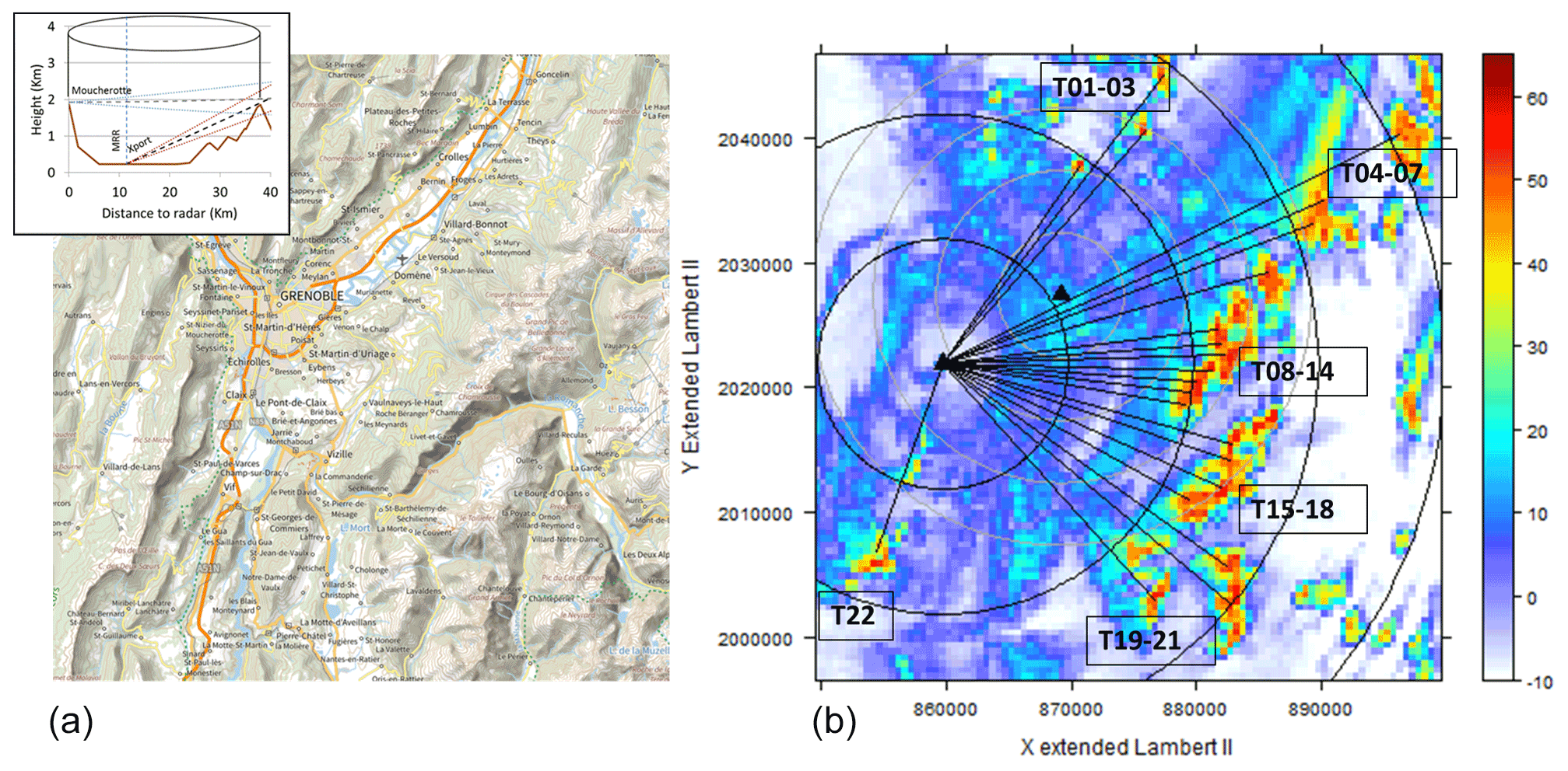
Figure 1(a) The 50×50 km2 map of the region of Grenoble, France (from Geoportail, Institut Géographique National). (b) Dry weather reflectivity map of the X-band weather radar located on top of the Moucherotte mountain (1901 m a.s.l.) in the Vercors Massif. The radar is marked with a black triangle, and circular range markers are spaced by 10 km. The Cartesian map has a resolution of 500 m. The measurements were taken at an elevation angle of 0∘ during dry weather conditions before the 21 July 2017 event. The radial lines indicate the azimuths and ranges of the 22 mountain targets used for the MRT implementation. Targets 1–3 are located in the Chartreuse Massif, targets 4–14 in the Belledonne Massif, targets 15–21 in the Taillefer Massif and target 22 in the Vercors Massif. In the background, the second black triangle indicates the IGE site at the bottom of the valley (210 m a.s.l.). The grey circles with 5 km spacing indicate the coverage of the XPORT X-band polarimetric radar, whose measurements were used in the present study only for the detection of the melting layer.
The article is organized as follows. In the theoretical part (Sect. 2), we find it useful to revisit in some detail the physics of propagation and attenuation of microwaves in rain. We derive (Sect. 2.2) four attenuation–reflectivity (AZ) algorithms constrained or not by path-integrated attenuations (PIAs) estimated from the decrease in the return of selected mountain targets when it rains, compared to their dry weather levels. We also consider a simple polarimetric algorithm based on the profile of the total differential phase shift between the radar and the mountain targets (Sect. 2.3). The structure and interdependencies of the parameters are discussed in Sect. 2.4. This leads to the description of the principles of the generalized sensitivity analysis proposed for studying the physical model at hand (Sect. 3.1). The results obtained are illustrated and discussed, item by item, in Sect. 3.2.1–3.2.5. Concluding remarks and future work are presented in Sect. 4.
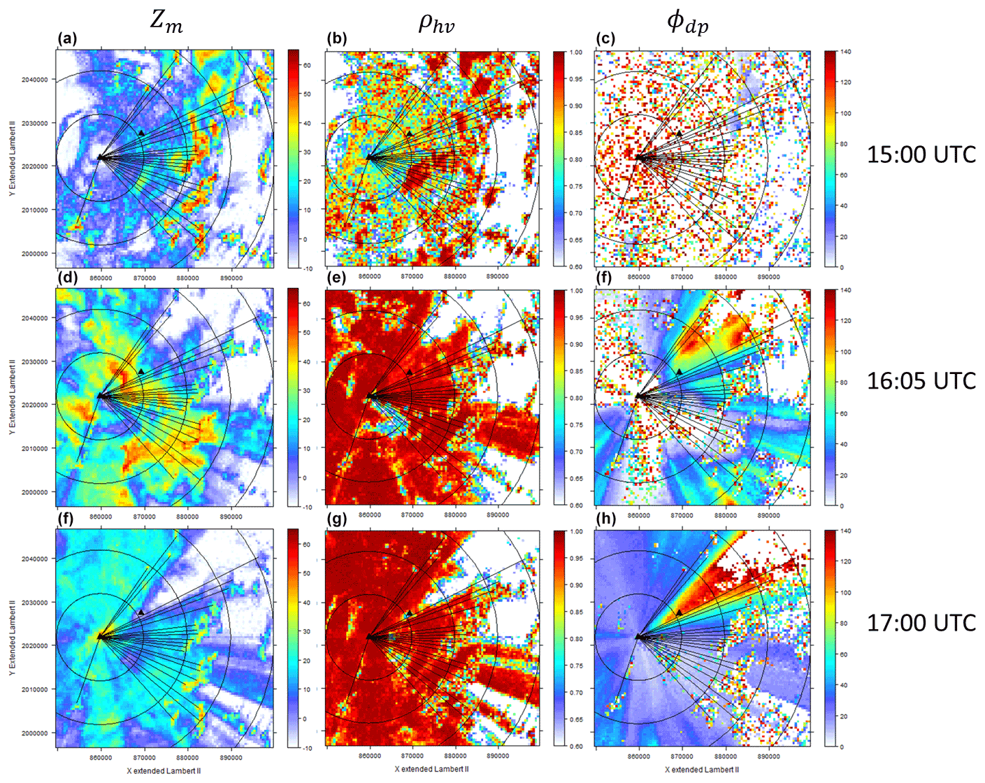
Figure 2Examples of 0∘ elevation PPIs of measured reflectivity (a, d, f), co-polar correlation coefficient (b, e, g) and total differential phase shift (c, f, h) taken before (a, b, c) and at two moments with intense precipitation (d–h) during the 21 July 2017 convective event. As in Fig. 1, the circular range markers of the Moucherotte mountain radar are spaced by 10 km.
2.1 Basic definitions and notations
Let us express the radar returned power profile P(r) (mW) as follows:
where Z(r) (mm6 m−3) is the true reflectivity profile, AF (r) (–) is the attenuation factor at range r (km), and C is the radar constant. We suppose the measured reflectivity profile Zm(r) to depend both on the attenuation and on a possible radar calibration error denoted dC as follows:
In addition to the running range r, let us consider the range r0 corresponding to the blind range of the radar system, which is eventually extended to the range where the reflectivity measurements start to be free of spurious detections due, e.g., to side lobes.
The attenuation factor AF(r) is expressed as the product of two terms in the following:
where AF(r0) is the on-site attenuation factor which, as discussed in the introduction, may result from two main sources, i.e. attenuation due to a water film on the radome and along-path attenuation due to precipitation falling between the radar site and range r0.
As a classical formulation (e.g. Marzoug and Amayenc, 1994), we express the two-way attenuation factor as a function of the specific attenuation profile A(r) (dB km−1) through the following equation:
Furthermore, we have to introduce relationships between the radar measurable variables (specific attenuation and reflectivity) and the variable of interest for QPE, i.e. the rain rate R (mm h−1), which are assumed to be of power type with the following notations:
The order used for the variables in Eqs. (2.5)–(2.7) is meaningful, since the specific attenuation profile is derived from the measured reflectivity profile, while the rain rate profile can be derived in a second step either from the specific attenuation profile or from the corrected reflectivity profile. Due to the well-known lower variability of the R–A relationship compared to the R–Z relationship, Eq. (2.6) is preferred to Eq. (2.7) for the estimation of the rain rate profiles (Ryzhkov et al., 2014).
Let us now consider another particular range, denoted as rm, where estimates of the attenuation factor may be available. We use the following notation:
where AF(rm) is the true attenuation factor at range rm, and the term dAFm represents a multiplicative error term. As illustrated in the introduction, such direct estimates of the attenuation factor can be obtained in mountainous regions using the mountain reference technique (MRT).
We frequently use hereinafter the notion of path-integrated attenuation (PIA), in units of decibels (hereafter dB), defined as follows:
Note that, since AF(r) is comprised between 1 (no attenuation) and 0 (full attenuation), the PIA subsequently takes values in the range of 0 (no attenuation) up to +∞ (full attenuation). The PIAs at ranges r0 and rm are denoted as PIA0 and PIAm, respectively, in the following.
2.2 Formulation of the attenuation–reflectivity algorithms
The following mathematical developments are inspired by the works on rain-profiling algorithms in satellite measurement configuration (e.g. Meneghini et al., 1983; Marzoug and Amayenc, 1994). The attenuation–reflectivity algorithms (AZ algorithms) proposed in this section rely on two basic equations. The first one is the analytical solution of Eq. (2.4), when the power law model (Eq. 2.5) is supposed to represent perfectly the A–Z relationship. By taking the derivative of with respect to range r, one obtains the following:
Substitution of the true reflectivity by the measured reflectivity through Eq. (2.2) and integration between r0 and r yields the following:
with
The second equation is obtained by integrating Eq. (2.10) up to range rm and by introducing the attenuation factor estimate available at this range, yielding the following:
We develop, in Appendix A, four formulations of attenuation corrections for a supposedly homogeneous precipitation type, i.e. we assume the aAZ and bAZ coefficients to be constant along the propagation path. Each formulation filters out one of the four parameters PIAm, dC, aAZ and PIA0, respectively. Note that, due to the mathematical expression of the intervening equations, there is no possibility to filter out the bAZ parameter, which will be assumed to be constant, close to a value of 0.8 at the X-band (Ryzhkov et al., 2014), and to present a low sensitivity in the system of equations. The resulting expressions of the reflectivity and specific attenuation corrected profiles are listed hereafter.
2.2.1 AZhb algorithm (independent of PIAm)
This formulation is equivalent to the solution proposed early by Hitschfeld and Bordan (1954), hence the proposed name AZhb. It can be termed as a forward algorithm since only the measured reflectivities between the range r0 and the running range r are used for the correction at range r. The minus sign between the two terms of the denominator indicates that the denominator is not prevented from tending towards 0 when the SZ cumulative term increases. This solution is subsequently known to be unstable and highly sensitive to calibration error, inadequate values of the A–Z relationship coefficients and on-site attenuation.
2.2.2 AZC algorithm (independent of dC)
In addition to its independence with respect to dC, it is interesting to note that the specific attenuation profile provided by the AZC algorithm does not depend on the aAZ parameter. This parameter is, however, present in the expression of the reflectivity profile.
2.2.3 AZα algorithm (independent of aAZ)
We note that the specific attenuation profiles provided by the AZC and AZα algorithms are identical. Moreover, they do not depend on the aAZ and dC parameters. This is a priori a very interesting property of these algorithms, exploited in particular by Testud et al. (2000) and Ryzhkov et al. (2014). However, the reflectivity profiles provided by the two algorithms are different, and in particular, the reflectivity profile of the AZα algorithm depends on dC, while the reflectivity profile of the AZC algorithm depends on aAZ.
2.2.4 AZ0 algorithm (independent of PIA0)
The AZ0 algorithm has the simplest mathematical expressions among the three algorithms using the PIA constraint. It looks like a backward algorithm, since the reflectivity and the specific attenuation profiles estimated at the running range r depend only on the measured reflectivities between ranges r and rm, while the AZC and AZα algorithms make use of the entire measured reflectivity profile between r0 and rm for the estimations at range r.
The plus (+) signs in the denominators of Eqs. (2.15)–(2.20) are indicators of the inherent stability of the three algorithms using the PIA constraint, unlike the AZhb algorithm.
2.3 Formulation of a polarimetric algorithm
In addition to the AZ algorithms, we consider a PIA profile, denoted as PIAΦdp(r0,r), derived from the profile of the total differential phase shift on propagation, denoted as Φdp(r0,r) (∘) in the following:
where Kdp is the specific differential phase shift on propagation (∘ km−1). Assuming a power law relationship between the specific attenuation and the specific differential phase shift on propagation, with the following:
We obtain the following:
This polarimetry-derived PIA profile can be compared to the PIA profiles obtained by integrating the AZ specific attenuation profiles given by Eqs. (2.14), (2.16), (2.18, which is identical to 2.16) and (2.20) between r0 and r.
2.4 Analysis of the parameters of the considered physical model
Equations (2.11), (2.12), (2.9) and (2.23) form a system of equations with seven parameters (or unknowns), namely the coefficients of the A–Z relationship (aAZ, bAZ), the coefficients of the A–Kdp relationship (aAK, bAK), the radar calibration error (dC), the on-site attenuation (PIA0) and the path-integrated attenuation at range rm (PIAm). We focus in this article on the idea of constraining this system of equations with the PIAs derived from the mountain reference technique. The question of the R–A transformation is beyond the scope of the present study.
From a physical point of view, the parameters dC, PIA0 and PIAm are mutually independent and a priori independent of the coefficients of the Z–A–Kdp power law models.
We will assume the radar calibration error to be constant for a given precipitation event, with possible variations from one event to the next.
Regarding on-site attenuation, Frasier et al. (2013) made a synthesis of previous theoretical and empirical studies and provided an empirical model based on the comparison of the measurements of two X-band radar systems in the French southern Alps, where one is equipped with a radome, and the other one is without a radome. From this article, we take into account a dependence of PIA0 on the measured reflectivity in the vicinity of the radar site, denoted as Z0. Based on Fig. 5 in Frasier et al. (2013), we have fitted a coarse power law model for X-band radome attenuation on their experimental data, yielding , with in decibels and Z0 in decibels relative to 1 mm6 m−3 (hereafter dBZ). Based on their Fig. 6, which shows important variations between the theoretical and empirical results proposed in the literature, we have defined a large range of lower and upper limits for the PIA0 draws conditioned on Z0 via the model (see Table 1). With n=5, the crude model proposed yields upper limits of the PIA0 sampling range of 4.8, 9.2, 14.6 and 20.8 dB for Z0 values of 20, 30, 40 and 50 dBZ, respectively. In the following simulations, PIA0 will be allowed to vary from one target to the next, i.e. in different directions, and from one time step to the next.
Table 1Values and ranges of the variation in the attenuation model parameters in the sensitivity analysis.
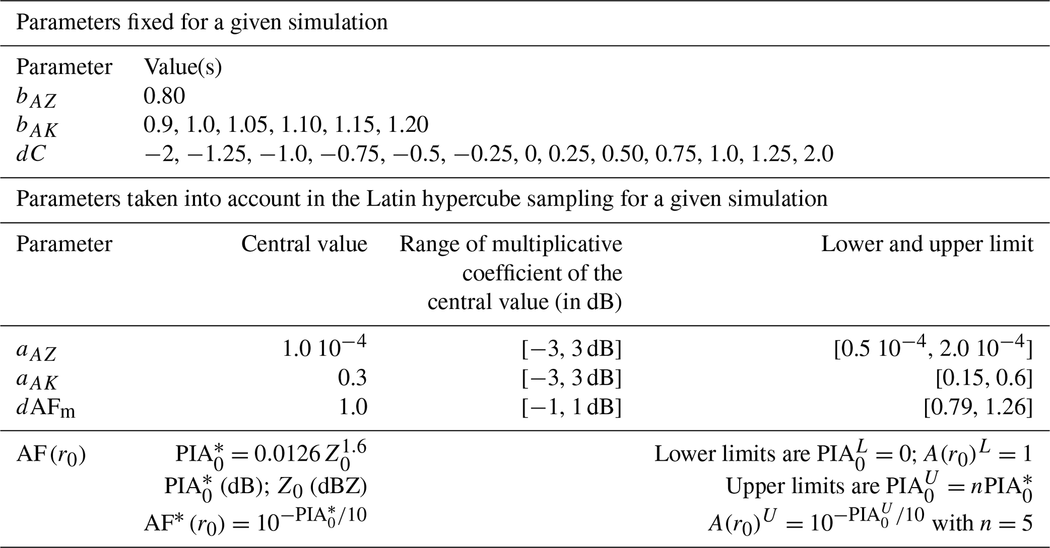
The accuracy of the MRT-derived PIAm was studied in Delrieu et al. (1999a) by comparing MRT estimates with direct measurements obtained with a receiving antenna set up in the mountain range. They showed (i) that selecting strong mountain returns (typically greater than 45–50 dBZ) allows one to mitigate the impact of precipitation falling over the target (negative bias), (ii) that a refined estimation of the so-called dry weather baseline is required to account for the possible modification of backscattering properties of the mountain surfaces before and after the event and (iii) that the time variability in the dry weather returns defines the minimum detectable PIA. These elements were accounted for in the present study by selecting strong mountain targets, studying their dry weather time variability (see also Delrieu et al., 2020) and subsequently defining the range of variation in the dAFm multiplicative error (Table 1).
The prefactors and exponents of the Z–A–Kdp power law models are mutually dependent, since they are determined by the shape, density and size distributions of the hydrometeors and their electromagnetic properties, which are largely driven by their solid versus liquid composition. These coefficients may vary considerably from one precipitation type to another. In addition, even for a given precipitation type, the actual Z–A–Kdp values present an inherent variability with respect to the power law models, associated with the greater or lesser proximity of the particle size distribution (PSD) moments associated to each particular variable. As a further complexity, when, for a given propagation path, various types of hydrometeors are successively encountered (e.g. rain, melting precipitation and snow), it would be desirable to apply the appropriate coefficients for the different precipitation types, provided one is able to determine them. As a major simplification in the present work, we will be considering a homogeneous precipitation type (convective rainfall). Because of the mathematical form of the equations at hand, and the likely mutual dependence of the exponent and prefactor of each power law model, we will assume the exponents of the A–Z and the A–Kdp relationships to be constant for all the considered events, while the prefactors will be allowed to vary for each single target and time step.
There have been several studies deriving A–Z and A–Kdp relationships at the X-band using different approaches, including model calculations and also the direct use of observational data (e.g. Bringi and Chandrasakar, 2001; Gorgucci and Chadrasakar, 2005; Park et al., 2005; Schneebeli and Berne, 2012; Matrosov et al. 2014; Yu et al., 2018). Estimations of these coefficients and their ranges in variation were obtained in our study by processing the drop size distribution (DSD) data collected with a Parsivel2 disdrometer located at the IGE site. The dataset includes 337 rainy days during the period April 2017–March 2020. The raw DSD measurements have a time resolution of 1 min. They are binned into 32 diameter classes with increasing sizes from 0.125 mm up to 6 mm. Various filters have been applied to discard anomalous data and, in particular, to detect non-liquid precipitation, thanks to the falling speed spectra. The volumetric concentration spectra have been computed at a 5 min resolution. DSD spectra with 5 min rain rate less than 0.1 mm h−1 were discarded from the analysis. A dataset of about 14 600 DSD spectra was thus obtained, corresponding to all types of precipitation occurring in liquid phase in the Grenoble valley. As for the scattering model, we used the CANTMAT version 1.2 software programme that was developed at Colorado State University by C. Tang and V. N. Bringi. The CANTMAT software uses the T-matrix formulation to compute radar observables such as horizontal reflectivity, vertical reflectivity, differential reflectivity, co-polar cross-correlation, specific attenuation, specific phase shift, etc., as a function of the DSD, the radar frequency, air temperature, oblateness models and canting models for the raindrops, as well as the incidence angle of the electromagnetic waves. The results presented herein were computed for the X-band frequency, a temperature of 10 ∘C, the Beard and Chung (1987) oblateness model, a standard deviation of the canting angle of 10∘ and an incidence angle of 0∘ (horizontal scanning, as for the MOUC radar data).
Figure 3 illustrates the fittings of the A–Z relationships that can be obtained from a classical logarithm of a base 10 transformation of the two variables. One can note that the scatterplot is well conditioned for deriving a power law model in the sense that it does not present any particular curvature. The least square regressions of A over Z and of Z over A, as well as the least rectangle regression, are displayed to illustrate the impact of the regression technique on the model coefficients. Note that the least rectangle fit should be preferred, since, for these calculations based on DSD data, the two variables can be considered to be on an equal footing. The determination coefficient is high, and the three regressions performed subsequently give parameter sets close to each other. From the fittings in Fig. 3, we have chosen bAZ=0.8 as a fixed value for this exponent and as the central value for the sampling of the prefactor in the following sensitivity analysis. Although the scatter of the points around the power law model suggests a possible range of variation of [−5, 5 dB] for the DSD-derived values, we have limited this range to [−3, 3 dB] in our simulations on the basis of the much bigger resolution volume of the radar and the assumption that the prefactor is constant throughout the reflectivity profile (Table 1).
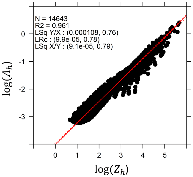
Figure 3Results of the fitting of DSD-derived power law models for the horizontal specific attenuation Ah (dB km−1) as a function of the horizontal reflectivity Zh (mm6 m−3), using a classical logarithmic of base 10 transformation of the two variables. In the insert, the number of points N, the square of the correlation coefficient (R2) of the logarithmic regression, the prefactors and exponents of the resulting least square regressions of the variable in ordinate versus the variable in abscissa (Lsq ) and vice versa (Lsq ), as well as the least rectangle regression (LRc), which considers the two variables on an equal footing, are shown.
Figure 4 gives the results obtained for the A–Kdp relationship. It can be seen that the scatterplot of the logarithmic of base 10 transformed variables (Fig. 4a) presents a significant curvature. Due to the important weight given to low and medium values in the regressions, the fitted power law models are clearly unsatisfactory for the highest values, which are of interest in the present study since they correspond to convective precipitation. We have therefore tested two other fitting techniques based on the natural values of the two variables (Fig. 4b). A linear fit with a zero-forced intercept yields Ah=0.32 Kdp, which is consistent with linear relationships proposed in the literature in similar climatological contexts; however, these are with a somewhat higher value of the multiplicative coefficient (e.g. 0.245 in Schneebeli and Berne (2012) and 0.276 in Yu et al. 2018). However, we note that this linear fit is not satisfactory with a significant underestimation of the Ah values for Kdp>3 ∘ km−1. The fitting of a non-linear power law model (NLPL) proves to be more satisfactory with . Since the exponents estimated with the log-transformed data are close to 0.9, we have decided to perform several simulations with fixed values of bAK in the range [0.9–1.2] (see Table 1). Regarding the prefactor aAK, we have considered a central value of 0.3 and a range of variation of [−3, 3 dB], with minimum and maximum values of 0.15 and 0.6, respectively.

Figure 4Fitting of DSD-derived power law models for the horizontal specific attenuation Ah (dB km−1) as a function of the specific differential phase shift on propagation Kdp (∘ km−1) (a) using a classical logarithmic of base 10 transformation of the two variables (same comments as in Fig. 3 for this graph) and (b) using natural values of the two variables. The red line in panel (b) is the zero-forced linear regression with a slope equal to 0.32, and the blue curve is the non-linear fit of a power law model with a prefactor of 0.30 and an exponent of 1.1.
Additional tests have been performed, including, for instance, the influence of the air/hydrometeor temperature, the precipitation type (e.g. stratiform versus convective rainfall) and the DSD integration time step. Concerning the last factor, we have compared the results obtained for the 2 and 5 min time steps, and we have found no significant influence on the coefficients of the power law models, while the R2 values were significantly downgraded for the 2 min time step (not shown here for the sake of conciseness). As for the precipitation type, we carried out a rough classification of the 337 events into stratiform and convective types by considering an event as convective if a rain rate threshold of 10 mm h−1 was exceeded for at least one 5 min time step during the event. As one would expect from the scatterplots in Figs. 3 and 4, significant differences appeared between the stratiform and convective A–Kdp relationships, whereas the A–Z relationships were almost identical. This is an argument for keeping the exponent bAZ constant in our simulation procedure. Regarding the sensitivity on temperature, one possible extension of the present work could be to consider the temperature time series available for each event at the IGE site in the scattering calculations. This would most likely result in an increase in the variability of the A–Z and A–Kdp relationships. As a classical concern, one may, however, wonder how the average temperature in the radar resolution volume could be estimated (Ryzhkov et al., 2014). We chose herein to rely on the ability of the simulation procedure to deviate from the central values of the parameters and their ranges of variation defined in Table 1 to be large enough.
3.1 Principle
The parameter structure analysed in Sect. 2.4 led us to organize the sensitivity analysis procedure in a nested way.
For all the considered rain events, we assume the exponents of the A–Z and A–Kdp relationships to be constant. For each event, we assume the radar calibration error to be constant. A simulation is performed for each combination of the bAZ, bAK and dC values listed in Table 1, i.e. simulations.
For each mountain target and each time step, the simulation core is implemented as follows.
The Zm(r) and Φdp(r) profiles between the radar and the mountain target are preprocessed. For each of the successive radials composing the target, this includes the determination of gates affected by clutter in the region of the mountain target and along the propagation path. This is done by considering both dry weather mean values exceeding various thresholds (25 dBZ for significant clutter; 45 dBZ for a gate belonging to the mountain target) and by using the profile of the co-polar correlation coefficient (ρhv) (Delrieu et al., 2020). The median Zm(r) and Φdp(r) profiles over the series of radials are then computed. The MRT PIAm is evaluated as being the difference in the Zm mean values between the dry weather baseline and the current time step, with the mean being taken over by all the gates composing the target. The r0 value is estimated as the range of the first gate for which four successive values (corresponding to a range extent of 960 m) exceed a ρhv value of 0.95. This last value is set as a threshold between precipitation and clutter/no precipitation (from the statistics presented in Khanal et al., 2019). The Z0 value is computed as the product of (correction for the radar calibration error) and the mean reflectivity of the selected four successive gates if they are located within the first 2 km range; otherwise, the Z0 value is set to 0. The reader is referred to Khanal et al. (2022) for the most recent description of the fairly sophisticated procedure used for the Φdp(r) regularization based on the total differential phase shift profiles Ψdp(r) for all the radials associated with a given target. Note that a target is selected at a given time step for the following steps of the simulation if PIAm> 1 dB and if a good quality index of the Φdp(r) regularization is obtained (Khanal et al., 2022).
The Latin hypercube sampling (LHS) technique (https://cran.r-project.org/web/packages/lhs/index.html, last access: 19 May 2022) is then used to generate N parameter sets (with N = 1000 in the following) filling uniformly the parameter space composed of the following four parameters: the prefactors aAZ and aAK, the on-site attenuation factor AF(r0) and the multiplicative error dAFm (Eq. 2.8) on the MRT attenuation factor. The central values and intervals of variation in these four parameters are listed in Table 1. It is noteworthy that the random draws are made on the decibel-transformed (db-transformed) ranges of parameters so that there are as many values below and above the central value, e.g., as many values between 0.15 and 0.3, on the one hand, and between 0.3 and 0.6, on the other hand, for the aAK parameter.
After discarding unphysical parameter sets (e.g. those for which PIA0>PIAm), the five algorithms are implemented for all the remaining sets. A cost function (CF) is evaluated in order to measure the convergence/proximity of the simulated profiles for each parameter set. Several formulations of the cost function were tested, and we propose the following one hereinafter, which was found to be appropriate:
where “Mean” stands for the mean value of something, and R2 is the determination coefficient between the two profiles indicated between parentheses. The profiles considered in this expression of the cost function are the PIA profiles between ranges r0 and r. Since the specific attenuation profiles are identical for the AZC and AZα formulations (Eqs. 2.16 and 2.18), only the PIA profile of the first is considered in Eq. (3.1). Due to the inherent instability of the AZhb algorithm, we consider the first three R2 terms in the computation of the CF value only if PIAm < 10 dB. Indeed, this 10 dB value proved to be about the maximum PIA that this algorithm is able to deal with, even with an almost perfect parameterization (Delrieu et al., 1999b). The last three terms of the CF are measuring the proximity of the three PIA-constrained algorithms. In the following, we have selected CFth=0.8 as the satisfaction threshold, i.e. the CF value to be exceeded to consider a given parameter set as being optimal.
The acronym OPS will be used to denote the optimal parameter set hereinafter. The number of optimal parameter sets (NOPSs) can be computed for a given target and time step and summed up for all the targets and time steps of an event and for a series of events to yield a measure of the overall quality of a simulation for given fixed parameters (bAZ, bAK and dC) and randomly drawn parameters (aAZ, aAK, AF(r0) and dAFm) for each single target/time step using the Latin hypercube sampling (LHS) technique. We recognize that the choice of the cost function (Eq. 3.1) and the satisfaction threshold CFth are essentially subjective. This choice relies on the experience gained in the implementation of the simulation framework. The following three elements can be mentioned on this subject: (i) accounting for the AZhb algorithm in the CF for low to moderate PIAs less than 10 dB proved to be a good option owing to the strong sensitivity of this algorithm on the calibration error; (ii) adding the polarimetric algorithm and the corresponding R2 terms in the CF allowed us to dramatically reduce the mathematical ambiguity (i.e. the fact that several combinations of parameters, including non-physical values, may lead to the convergence of the solutions of the different algorithms) of the physical model at hand; and (iii) several satisfaction thresholds were tested with low sensitivity on the results in terms of the quantiles of the statistical distributions of the estimated parameters.
3.2 Results
3.2.1 Illustration for a given target and time step
Figure 5 gives an example of result of the core procedure for target 13 (T13) on 21 July 2017 16:05 UTC. For this case, with a MRT PIA of 25.9 dB at a range of about 20 km, we obtain ∘ and Z0= 9.5 dBZ. The optimal set of fixed parameters for the considered event is dB, bAZ=0.8 and (see the next sub-sections). Since, for the best OPS, all the profiles overlap perfectly, the results presented in Fig. 5 correspond actually to a near-optimal set so that one can see some differences between the solutions of the different algorithms. The set of LHS parameters for this specific target/time step is dB, , and . The CF value is 0.925, while the one obtained with the best OPS is 0.981. Note that 55 parameter sets overpassed the CF threshold value of 0.8 for this example, i.e. NOPS = 55 for this target and time step. For this good (though not the best) OPS, the reflectivity profiles (Fig. 5a) call for the following comments. We have here a clear example of the inherent instability of the AZhb algorithm, which blows up at a range of about 7 km for this parameterization. One should remember that this algorithm is not accounted for in the CF computation for such high PIAs, as explained when commenting on Eq. (3.1). The three other AZ algorithms give rather similar results. As a general behaviour (and in particular whatever the value of the on-site attenuation), we note that the optimal parameterizations lead to the convergence of the AZC and AZ0 algorithms near the radar and to the convergence of the AZα and AZ0 algorithms at the other end of the profile. Figure 5b gives the solutions obtained in terms of specific attenuation profiles. The AZhb profile is not drawn in this figure. As shown in Sect. 2.2, the AZα and AZC solutions are identical (represented in red) and slightly different at a long range from the AZ0 solution. The comparison of the corrected and uncorrected profiles clearly shows in this example the dramatic impact of attenuation with regard to both the underestimation of the first precipitation cell and the non-detection of the second one. Figure 5c displays the raw and processed Φdp profiles. For such a strong attenuation case, one can see that the raw profile has little noise and no significant bumps that could signify a differential phase shift on backscattering (δhv) contamination (Trömel et al., 2013). Finally, Fig. 5d allows a comparison of the PIA profiles derived from the AZC–AZα algorithms (identical solutions), the AZ0 algorithm and from the Φdp profile. Although there are some differences, the overall consistency between the three profiles is good.
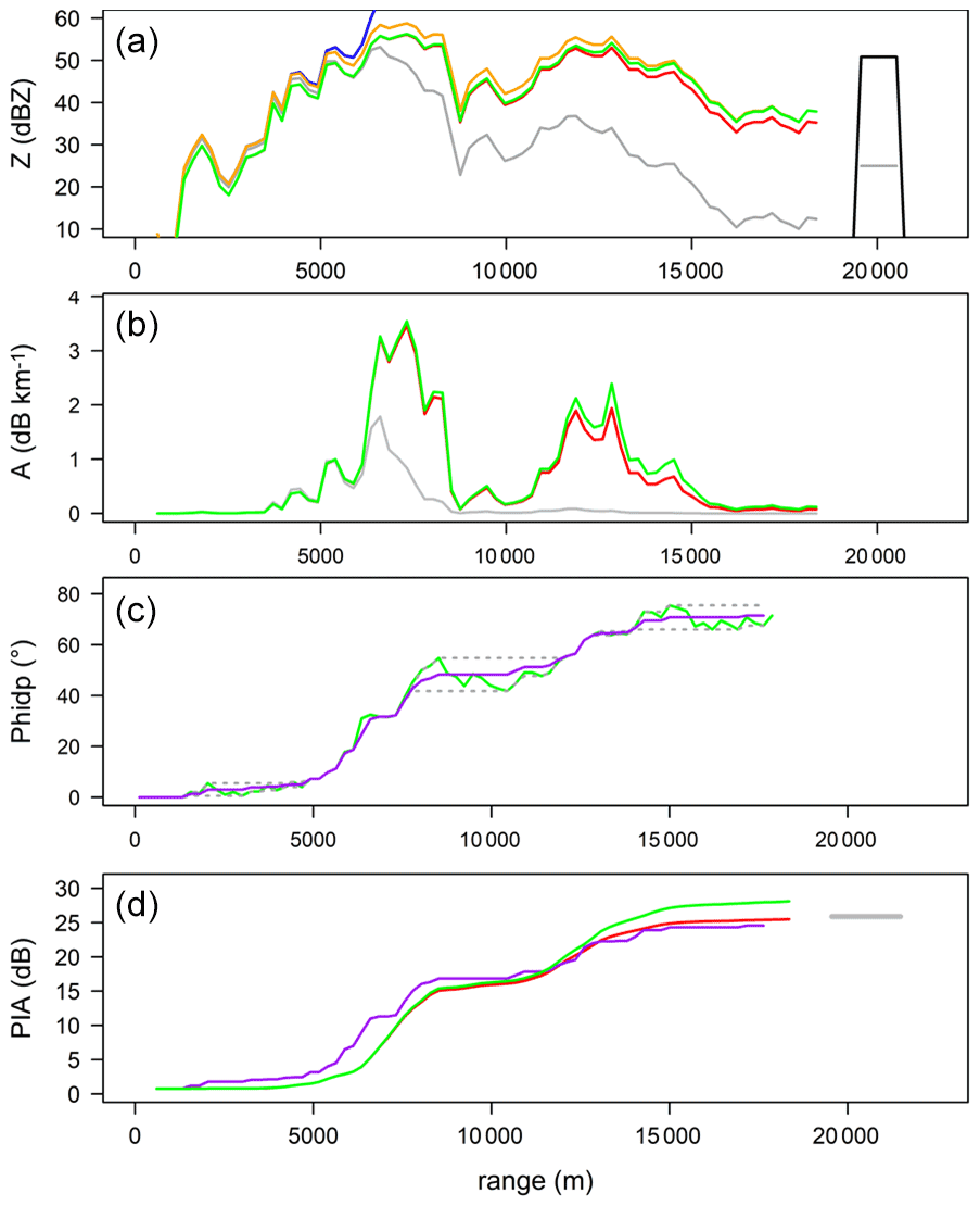
Figure 5Implementation of the five algorithms (blue – AZhb; red – AZC; orange – AZα; green – AZ0; purple – PIAϕdp) for mountain target T13 during the 21 July 2017 convective event at 16:00 UTC using a near-optimal parameter set (see text for details). The results are displayed in terms of profiles of (a) reflectivity, (b) specific attenuation, (c) differential phase shift on propagation and (d) path-integrated attenuation. The grey profile in panel (a) is the measured reflectivity profile; the black and grey horizontal lines at range 20 km represent the mean dry weather baseline and current reflectivities, respectively, of the mountain target. The resulting measured PIA value of 25.2 dB is reported in grey in panel (d). The grey profile in panel (b) is derived from the measured reflectivity profile by using Eq. (2.5). The purple line in panel (c) is the raw total differential phase shift profile, and the grey dotted curves are the envelope curves used in the regularization procedure (Delrieu et al., 2020; Khanal et al., 2022).
3.2.2 Time series of optimal parameter values
Figure 6 presents the time series of quantiles of the distributions of the input variables and the estimated optimal parameters obtained for the best simulation of the 21 July 2017 convective event. The sampling strategy making use of Z0 (see Table 1) is considered for PIA0. We will come back, in Sect. 3.2.5, to the relationship between PIA0 (Fig. 6c) and Z0 (Fig. 6a). The medians of PIAm and Φdp(r0,rm) (Fig. 6b) give an indication on the evolution of the storm which was intense between 15:30 and 17:00 UTC, with medians of about 20 dB and 60∘, respectively. The interquartile ranges of these two variables are quite large, as a result of both the variation in the radar target distances (from 15 up to 40 km) and the precipitation variability as a function of the azimuth, illustrated in Figs. 1 and 2. The time evolution of the storm intensity is also visible on the NOPS time series (Fig. 6f), with multiplicative factors in the range of 5 to 10 between the period 16:00–17:00 and the period 17:00–18:00 UTC. Although, for a given target, there is an increasing trend of NOPS when PIAm increases (not shown for the sake of conciseness); this is also related to the higher number of targets reached (i.e. targets with PIAm values greater than 1 dB) between 16:00 and 17:00 UTC. The time series of the prefactors aAK (Fig. 6d) and aAZ (Fig. 6e) have a similar behaviour with rather stable median values that are close to the central values of the sampling intervals derived from the analysis of the DSD data (Sect. 2.4; Table 1). This is reassuring as to the relevance for radar data processing of these DSD-derived relationships deduced from in situ microphysical measurements and scattering models. We note, however, that the interquartile ranges are quite large, especially those of the aAZ parameter. This is an indication that the mathematical ambiguity (Haddad et al., 1995) of the system of equations at hand remains important. It is noteworthy to mention that the ambiguity of the AZ algorithms alone is much larger (e.g. with larger interquartile ranges for the aAZ parameter). Introducing the polarimetric algorithm and the associated constraints on the coefficients of the A–Kdp relationship allowed it to reduce dramatically (not shown for the sake of conciseness).
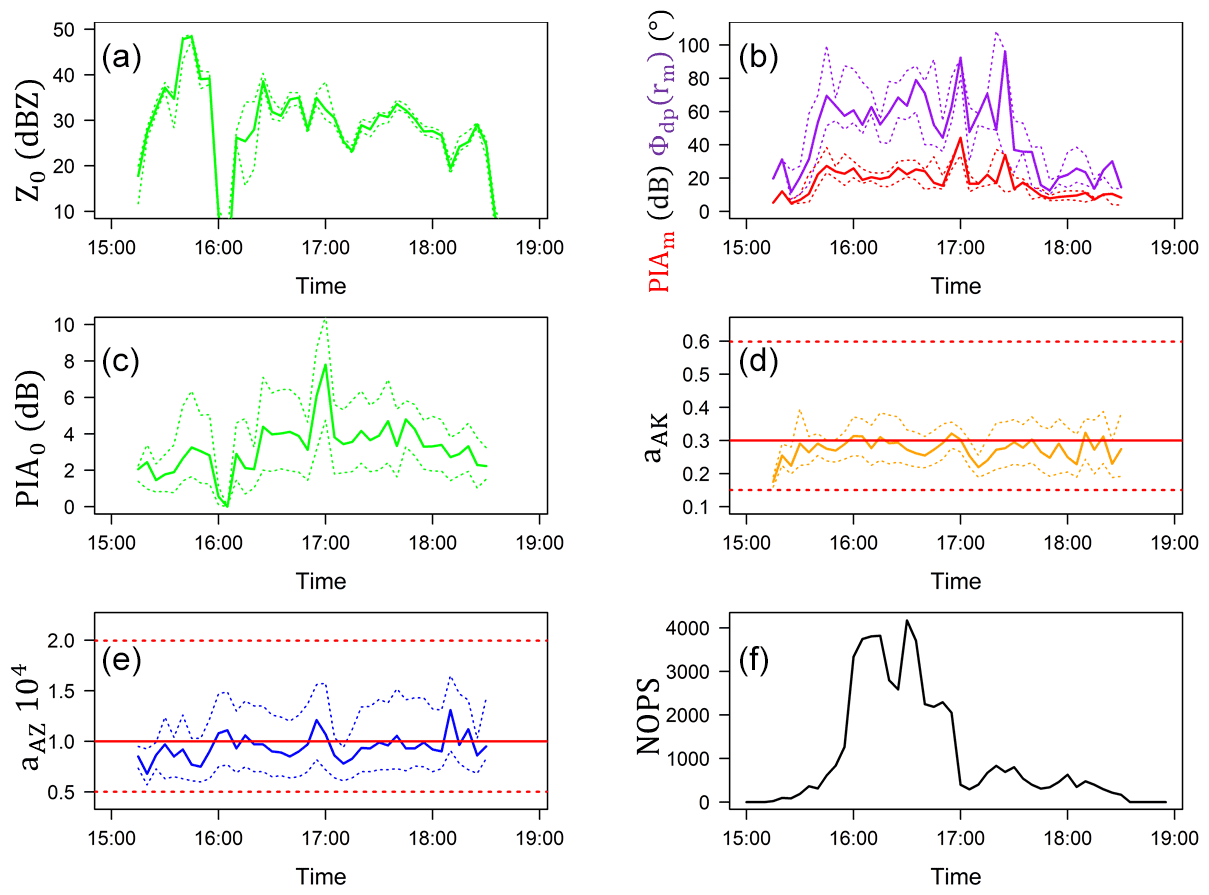
Figure 6Time series of the input variables and optimal parameters for the best simulation obtained for the 21 July 2017 convective event. The optimal set of fixed parameters for this event is dC = 0.5 dB, bAZ=0.80 and bAK=1.1. For each of the three considered input variables (a) Z0, (b) PIAm (red) and Φdp(r0rm) (purple) are displayed the median (continuous line) and the 25 % and 75 % quantiles (dotted lines) of their distributions over the 22 mountain targets. A similar representation is proposed for the LHS optimal parameters (c) PIA0, (d) aAK and (e) aAZ, except that the distributions are established over all optimal parameters of all targets. In panels (d) and (e), the dotted horizontal lines materialize the lower and upper limits consider in the LHS of the considered parameter. The time series of the number of optimal parameter sets (NOPSs) cumulated over all the 22 targets is displayed in panel (f).
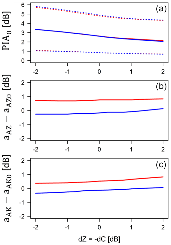
Figure 7Evolution of the medians of the distributions of on-site attenuation (a), prefactor of the A–Z relationship (b) and prefactor of the A–Kdp relationship (c) estimated for the 21 July 2017 event as a function of the calibration error. The variable dZ, equal to dC, is used to represent the dBZ value to be added to the measured reflectivities for correcting the calibration error. The prefactors, expressed in dB, are calculated with respect to the central values of their intervals of variation as follows: and aAK0=10 log(0.3) (Table 1). As in Fig. 4b, the red curves correspond to bAK=1, and the blue curves to bAK=1.1. The dotted red and blue curves in the top graphs represent the 25 % and 75 % quantiles of the distributions of PIA0.
Figure 7 presents additional results for the 21 July 2017 event with the evolution of the medians at the event timescale of estimated PIA0 (Fig. 7a), the prefactor of the A–Z relationship (Fig. 7b) and the prefactor of the A–Kdp relationship (Fig. 7c) as a function of the calibration error, for two values of the bAK exponent (1.0 and 1.1). For convenience, the variable dZ = − dC is used in Fig. 7 to represent the dBZ value to be added to the measured reflectivities for correcting the calibration error. We note that the calibration error has a significant impact on the median and interquartile range of PIA0, with, logically, stronger on-site attenuations for negative dZ values. The prefactors, expressed in dB relative to the central values in Fig. 7, show a slighter and opposite trend to increase as dZ increases. We also note the marked influence of the bAK exponent on the two prefactors, with an offset of about 0.9 and 0.65 dB on the medians of aAZ and aAK, respectively, for dZ = 0.

Figure 8Evolution of the total number of optimal parameter sets (NOPSs) as a function of the radar calibration error for three convective events separately (dotted blue curves) and all together (solid blue curve). The other fixed parameters for these simulations are bAZ=0.8 and bAK=1.1.
3.2.3 Estimating the radar calibration error
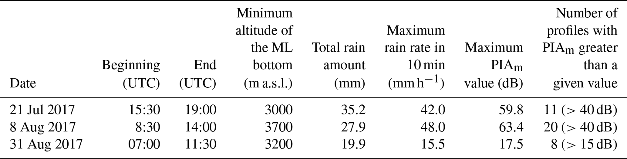
In order to increase the robustness of the results, the simulation procedure was performed for three convective events that occurred successively during summer 2017. Table 2 presents some characteristic features of these events. For all of them the melting layer (ML) altitude, determined with the 25∘ elevation XPORT radar data by using the procedure developed in Khanal et al. (2019), was situated well above the altitude of the Moucherotte mountain radar; hence, there is no ML contamination of the considered radar data. The first two events were rather intense and similar in terms of total rain amount and maximum rain rate at the IGE site and in terms of the PIAm statistics based on the 22 mountain targets. The third one was a bit less intense. To our knowledge, there was no occurrence of hail reported in the area of interest for these three events.
Table 2Some characteristics of the three convective events considered in this study. The melting layer (ML) detection was performed with the 25∘ elevation angle measurements of the XPORT radar, using the algorithm described in Khanal et al. (2019). The total rain amount and the maximum rain rate are recorded at the rain gauge available at the IGE site at the bottom of the Grenoble valley. The PIAm statistics are derived from the MRT by considering all the 22 mountain targets and the 0∘ elevation data of the Moucherotte mountain radar.
We propose to consider the total NOPSs obtained for a given simulation and for a given event as a quality criterion to judge the relevance of a set of fixed parameters (dC, bAZ and bAK). Figure 8 shows the NOPS evolution for the three events separately and all together as a function of the fixed values of dC, with the other fixed parameters being bAZ=0.8 and bAK=1.1 in this figure. We note that the various curves are rather flat near their optimum values. The overall sensitivity to the calibration error is clear, however, in the considered [−2, 2 dB] range, e.g., with a ratio of the maximum to the minimum NOPS values of 1.4 for the all-events curve. Although the global results tend to indicate an almost perfect calibration of the measured reflectivities (optimal dZ value in the following – of 0.25 dBZ), one can note that the dZ∗ values vary from one event to the next with −0.5 dBZ for the 21 July 2017 event, 1.0 dBZ for the 8 August 2018 event and 0.5 dBZ for the 31 August 2017 event. We find it difficult to know whether such variations in the electronic calibration of the radar from one event to the next are physically realistic. By eliminating the data from time steps with significant on-site attenuation, we checked that on-site attenuation could not be held responsible for these dZ∗ variations.
3.2.4 Linearity of the A–Kdp relationship
Similarly, Fig. 9 shows the evolution of the NOPS criterion computed for the three events all together as a function of the dZ and bAK (Table 1) values. We note a slight superiority of the simulations with bAK in the range [1.05–1.15] compared to the one with bAK=1.0 in terms of the NOPS maximum value. This observation is also valid for each of the three events separately (not shown for clarity in plotting). The simulation with bAK=0.9 is clearly below the other ones. For bAK=1.1 and for the optimal dZ value of each event, the log-transformed distribution of aAK computed over the three events is nearly symmetrical, with an average value of 0.28 and an interquartile range of about [−1, 1 dB]. Hence, we obtain in this study quite a remarkable agreement between the radar and DSD-derived A–Kdp relationships, with and , respectively. Similarly, the optimal A–Z relationship derived from the simulation exercise is very close to the one obtained by the DSD measurements (Fig. 3) with .
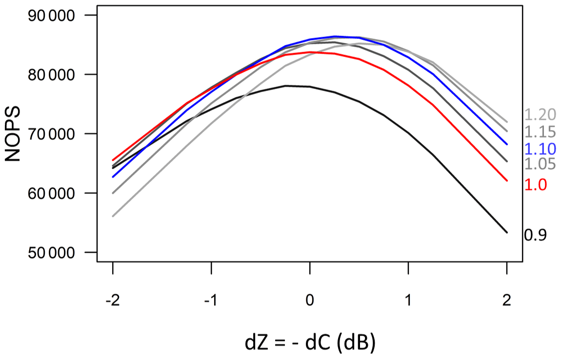
Figure 9Evolution of the total number of optimal parameter sets (NOPSs) computed for the three convective events all together as a function of dZ for various values of the exponent of the A–Kdp relationship listed on the right-hand side of the figure. As in Figs. 4b and 7, the red curve corresponds to bAK=1.0 and the blue curve to bAK=1.1.
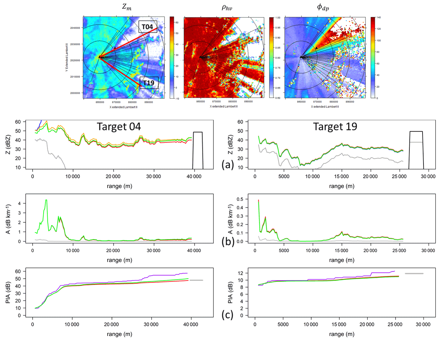
Figure 10Implementation of the five algorithms with sets of optimal parameters (blue – AZhb; red – AZC; orange – AZα; green – AZ0; purple – PIAϕdp) on 21 July 2017 at 17:00 UTC for mountain target T04, with both along-path and on-site attenuation (left), and for mountain target T19 with on-site attenuation mainly (right). The results are displayed in terms of profiles of (a) reflectivity, (b) specific attenuation and (c) path-integrated attenuation. In the upper images, the PPIs of the measured reflectivity (with the indication of the position of the two targets in red) are displayed together with the co-polar correlation coefficient and the raw total differential phase shift.
3.2.5 Radome attenuation
Coming back to Fig. 6, we remind the reader that the sampling strategy making use of Z0 was considered for the random drawing of PIA0 values in the simulation. One has to remark that such close-range reflectivity measurements are actually affected by radome attenuation. This may explain why estimated PIA0 values are higher for the time step at 17:00 UTC than for time steps between 15:30 and 15:55, while Z0 values are about 10 dBZ higher in the latter period. The relevance of the Z0 variable for detection and quantification of on-site attenuation remains limited for a radar equipped with a radome.
Figure 10 gives two examples of the core procedure implementation in the case of severe on-site attenuation that occurred on 21 July 2017 at 17:00 UTC (Fig. 2; bottom graphs). The constraint on the maximum value for the PIA0 sampling as a function of Z0 was relaxed in these calculations, with a maximum PIA0 limit set to 30 dB, whatever Z0. The mountain returns from target 04 (T04) allow us to quantify both on-site attenuation and along-path attenuation due to precipitation falling over the city of Grenoble (NE sector) at that time (left-hand side example). At this range of about 40 km, we obtain PIAm=47.9 dB and ∘. The mountain returns from target 19 (T19) located in the southeastern sector (right-hand side) seem to be essentially affected by the precipitation conditions at the radar site. At this range of about 27 km, we obtain PIAm=11.9 dB and ∘. This yields ratios of 0.37 and 0.97 dB ∘−1 for the two targets, respectively. These values are clearly (especially the second one) well above the range of expected values for the slope of a supposedly linear A–Kdp relationship. In addition to the generalized decrease in the mountain returns visible in Fig. 2, this is an indication of a large on-site attenuation effect. The dC-corrected Z0 values computed in the directions of the two targets are significantly different with 38.9 and 28.6 dBZ, respectively. One can observe the very good convergence of all the AZ algorithms in both cases. In particular for T19, all the AZ reflectivity profiles, including the AZhb one, are perfectly matched. The agreement is also very good between the PIA profiles of the AZ algorithms and the one of the polarimetric algorithm, except for a very slight stall of PIAΦdp(r) at a range of about 30 km for T04, likely due to disturbances associated with side-lobe effects (visible on the ρhv PPI on top of Fig. 10).
For the two OPS considered in Fig. 10, one obtains PIA0 values of 10.1 and 10.8 dB. By considering the PIA0 statistical distribution calculated over the optimal parameter sets of all the targets for the considered time step, one obtains a symmetrical distribution with a slightly higher mean value of 12.6 dB and a rather large interquartile range of 4.5 dB. The mean value increases somehow (13.5 dB) and the interquartile range decreases to 3.2 dB if the PIA0 distribution is computed for targets 9–22 only, i.e. for targets with reduced along-path attenuation. It is worth noting that such statistics are not improved (e.g. interquartile range reduced) if one considers a more stringent satisfaction criterion (e.g. CFth=0.9 instead of CFth=0.8).
In this article, we have started to implement a simulation framework to study the interactions between X-band microwaves and hydrometeors in a mountainous context. Emphasis was placed on the attenuation problem, which is known to be severe for the frequency under consideration and essentially impossible to correct unless estimates of total attenuation are available at a distance from the radar. The RadAlp experiment allows us to obtain direct PIA estimates from the mountain reference technique in some specific directions and indirect estimates from the processing of the profiles of total differential phase shift available for each radial. Although the polarimetric technique is a priori much more convenient to apply and has interesting characteristics (independence on radar calibration, on-site attenuation and partial beam blockages), it suffers from several limitations, including (i) the fact that the Ψdp profile is noisy for light precipitation, (ii) the possible contaminations by the differential phase shift on backscatter δhv, (iii) the possible impact of non-uniform beam filling and (iv) the need to specify the relationship between the specific attenuation and the specific differential phase shift which depends on hydrometeor types, temperature and so on. In a similar way to the satellite configuration (e.g. the possibility to use the surface reference technique in addition to the dual-frequency measurements at Ka and Ku bands for processing the radar data of the Global Precipitation Measurement (GPM) core platform; Meneghini et al., 2020), we have proposed taking advantage of all the MRT and polarimetric measurements available to perform a generalized sensitivity analysis of the physical model of interest. In the simple case of convective precipitation (i.e. without the contamination of the radar data by snow or melting precipitation), we have obtained interesting results regarding the estimation of radar calibration error, radome attenuation and the A–Z and A–Kdp relationships. We note that, for the estimated optimal radar calibration error, the A–Z and A–Kdp relationships derived from radar data are consistent with those derived from concomitant drop size distribution measurements at ground level, in particular with a slightly non-linear A–Kdp relationship (. This is reassuring regarding the relevance of the use of microphysical data and scattering models for the parameterization of radar data processing. We have deliberately left aside the question of the specific attenuation–rain rate conversion in this article. An interesting validation exercise to be performed consists of using the DSD-derived A–R relationship for the conversion of the estimated specific attenuation profiles. The resulting radar rain rate estimates will be compared with the rain gauge measurements available. Another outcome of the study is the quantification of X-band radome attenuation. Values as high as 15 dB were estimated, leading to the recommendation of avoiding the use of radomes for remote sensing of precipitation at such a frequency. As an alternative, it would be desirable to develop specific sensors to detect/quantify the presence of water on the radome wall (Mancini et al., 2018). As a next step, we plan to extend the procedure to stratiform events with MOUC radar measurements made at times within or above the melting layer. The multi-angle, multi-frequency, polarimetric measurements of the valley-based radars will be critical in this respect for the characterization of the ML from below (Khanal et al., 2019, 2022), the parameterization of Z–A–Kdp–R relationships for different hydrometeor types and the mitigation of the mathematical ambiguity of the physical model of interest.
A1 AZhb algorithm (independent of PIAm)
This formulation is based on Eq. (2.11) only. In other words, it does not make use of PIAm. By combining Eqs. (2.11), (2.2) and (2.3), one obtains a corrected reflectivity profile through the following equation:
The specific attenuation profile follows from the use of the A–Z power law model as follows (Eq. 2.5):
A2 AZC algorithm (independent of dC)
The attenuation constraint (Eq. 2.1.2.) is used to express dC as follows:
which is introduced in Eq. (2.11) to yield the following:
The corrected reflectivity profile is then derived from Eqs. (2.2), (2.3), (A.3) and (A.4) to read as follows:
Note that, in the previous derivations, the expression of dC given by Eq. (A.3) is used twice. It is used first in the expression of from Eq. (2.11) and then in the substitution of dC in Eq. (2.2).
The specific attenuation profile follows from the use of the A–Z relationship Eq. (2.5):
A3 AZα algorithm (independent of aAZ)
The attenuation constraint (Eq. 2.12) is used to express aAZ as follows:
which can be introduced in Eq. (2.11) to yield the following:
Equation (A.8) is actually identical to the expression (A.4). From Eqs. (A.8), (2.2) and (2.3), the resulting corrected reflectivity profile can be expressed as follows:
One can note that ZAZα(r) is different from ZAZC(r) (Eq. A.5) and that it depends on dC.
Next, it can be verified, by using Eqs. (A.9), (2.5) and (A.7) (a second time, for the necessary substitution of aAZ), that the AZα specific attenuation profile is identical to the AZC specific attenuation profile given by Eq. (A.6) with the following:
A4 AZ0 algorithm (independent of PIA0)
The attenuation constraint (Eq. 2.12) is used to express as follows:
which can be introduced in Eq. (2.11) to yield the following:
The resulting corrected reflectivity profile is as follows:
And the specific attenuation profile is as follows:
The code and data can be made available upon request to the authors.
GD is the main contributor for this article (concept, theoretical developments, calculations, article writing and corresponding author). AKK (doctoral student) and BB (assistant professor) are scientists contributing actively to the RadAlp experiment. They performed the internal review of the article. FC is a research engineer, who built and keeps improving the XPORT radar, a key instrument deployed in the RadAlp experiment. BB is also the Hydrométéorologie, Climat et Interactions avec les Sociétés (HMCIS) team leader and as such does a lot of work for all the team members.
The contact author has declared that neither they nor their co-authors have any competing interests.
Publisher’s note: Copernicus Publications remains neutral with regard to jurisdictional claims in published maps and institutional affiliations.
We thank the three anonymous reviewers, for their valuable comments, which helped us improving the article. We are grateful to P.N. Gatlin (NASA Marshall Space Flight Center, Huntsville, AL), for providing the CANTMAT version 1.2 software developed at Colorado State University by C. Tang and V.N. Bringi, who we also thank.
The RadAlp experiment is co-funded by the Labex osug@2020 of the Observatoire des Sciences de l'Univers de Grenoble, the Service Central Hydrométéorologique et d'Appui à la Prévision des Inondations (SCHAPI) and Electricité de France/Division Technique Générale (EDF/DTG).
This paper was edited by Gianfranco Vulpiani and reviewed by three anonymous referees.
Beard, K. V. and Chuang, C.: A new model for the equilibrium shape of raindrops, J. Atmos. Sci., 44, 1509–1524, https://doi.org/10.1175/1520-0469(1987)044<1509:ANMFTE>2.0.CO;2, 1987.
Bringi, V. N. and Chandrasekar, V.: Polarimetric Doppler weather radar, principles and applications, Cambridge University Press, 636 pp., ISBN 13 9780521623841, 2001.
Delrieu, G., Caoudal, S., and Creutin, J. D.: Feasibility of using mountain return for the correction of ground-based X-band weather radar data, J. Atmos. Ocean. Technol., 14, 368–385, https://doi.org/10.1175/1520-0426(1997)014<0368:FOUMRF>2.0.CO;2,1997.
Delrieu, G., Serrar, S., Guardo, E., and Creutin, J. D.: Rain Measurement in Hilly Terrain with X-Band Weather Radar Systems: Accuracy of Path-Integrated Attenuation Estimates Derived from Mountain Returns, J. Atmos. Ocean. Technol., 16, 405–416, https://doi.org/10.1175/1520-0426(1999)016<0405:RMIHTW>2.0.CO;2, 1999a.
Delrieu, G., Hucke, L., and Creutin, J. D.: Attenuation in rain for X- and C-band weather radar systems: Sensitivity with respect to the drop size distribution, J. Appl. Meteor., 38, 57–68, https://doi.org/10.1175/1520-0450(1999)038<0057:AIRFXA>2.0.CO;2, 1999b.
Delrieu, G., Khanal, A. K., Yu, N., Cazenave, F., Boudevillain, B., and Gaussiat, N.: Preliminary investigation of the relationship between differential phase shift and path-integrated attenuation at the X band frequency in an Alpine environment, Atmos. Meas. Tech., 13, 3731–3749, https://doi.org/10.5194/amt-13-3731-2020, 2020.
Foresti, L., Sideris, I. V., Panziera, L., Nerini, D., and Germann, U.: A 10-year radar-based analysis of orographic precipitation growth and decay patterns over the Swiss Alpine region, Q. J. Roy. Meteorol. Soc., 144, 2277–2301, https://doi.org/10.1002/qj.3364, 2018.
Frasier, S. J., Kabeche, F., Figueras i Ventura, J., Al-Sakka, H., Tabary, P., Beck, J., and Bousquet, O.: In-place estimation of wet radome attenuation at X band, J. Atmos. Ocean. Technol., 30, 917–928, https://doi.org/10.1002/qj.3366, 2013.
Germann, U., Galli, G., Boscacci, M., and Bolliger, M.: Radar precipitation measurement in a mountainous region, Q. J. Roy. Meteorol. Soc., 132, 1669–1692, https://doi.org/10.1256/qj.05.190, 2006.
Gorgucci, E. and Chandrasekar V.: Evaluation of attenuation correction methodology for dual-polarization radars: Application to X-band systems, J. Atmos. Ocean. Technol., 22, 1195–1206, https://doi.org/10.1175/JTECH1763.1, 2005.
Haddad, Z. S., Im, E., and Durden, S. L.: Intrinsic ambiguities in the retrieval of rain rates from radar returns at attenuating wavelengths, J. Appl. Meteor. Climatol., 34, 2667–2679, 1995.
Hitschfeld, W. and Bordan, J.: Errors inherent in the radar measurement of rainfall at attenuating wavelengths, J. Atmos. Sci., 11, 58–67, 1954.
Joss, J. and Lee, R.: The Application of Radar-Gauge Comparisons to Operational Precipitation Profile Corrections, J. Appl. Meteor., 34, 2612–2630, https://doi.org/10.1175/1520-0450(1995)034<2612:TAORCT>2.0.CO;2, 1995.
Khanal, A. K., Delrieu, G., Cazenave, F., and Boudevillain, B.: Radar remote sensing of precipitation in high mountains: detection and characterization of Melting Layer in French Alps, Atmosphere, 10, 784, https://doi.org/10.3390/atmos10120784, 2019.
Khanal, A. K., Delrieu, G., Cazenave, F., and Boudevillain, B.: Investigation of the relationship between path-integrated attenuation (PIA) and differential phase shift (Φdp) in the melting layer of precipitation at X-band frequency Atmospheric Measurement Techniques, in preparation, 2022.
Koffi, A. K., Gosset, M., Zahiri, E.-P., Ochou, A. D., Kacou, M., Cazenave, F., and Assamoi, P.: Evaluation of X-band polarimetric radar estimation of rainfall and rain drop size distribution parameters in West Africa, Atmos. Res., 143, 438–461, https://doi.org/10.1016/j.atmosres.2014.03.009, 2014.
Lengfeld, K., Clemens, M., Münster, H., and Ament, F.: Performance of high-resolution X-band weather radar networks – the PATTERN example, Atmos. Meas. Tech., 7, 4151–4166, https://doi.org/10.5194/amt-7-4151-2014, 2014.
Mancini, A., Salazar, J. L., Lebrón, R. M., and Cheong, B. L.: A novel instrument for real-time measurement of attenuation of weather radar radome including its outer surface. Part II: the concept, J. Atmos. Ocean. Technol., 35, 953–973, https://doi.org/10.1175/JTECH-D-17-0083.1, 2018.
Marzoug, M. and Amayenc, P.: A class of single and dual-frequency algorithms for rain-rate profiling from a spaceborne radar: Part 1 – Principle and tests from numerical simulations, J. Atmos. Ocean. Technol., 11, 1480–1506, https://doi.org/10.1175/1520-0426(1994)011<1480:ACOSAD>2.0.CO;2, 1994.
Matrosov, S. Y. and Clark, K. A.: X-Band Polarimetric Radar Measurements of Rainfall, J. Appl. Meteor., 41, 941–952, https://doi.org/10.1175/1520-0450(2002)041<0941:XBPRMO>2.0.CO;2, 2002.
Matrosov, S. Y., Kingsmill, D. E., Martner, B. E., and Ralph, F. M.: The Utility of X-Band Polarimetric Radar for Quantitative Estimates of Rainfall Parameters, J. Hydrometeor., 6, 248–262, https://doi.org/10.1175/JHM424.1, 2005.
Matrosov, S. Y., Campbell, C., Kingsmill, D. E., and Sukovich, E.: Assessing Snowfall Rates from X-Band Radar Reflectivity Measurements, J. Atmos. Ocean. Technol., 26, 2324–2339, https://doi.org/10.1175/2009JTECHA1238.1, 2009.
Matrosov, S. Y., Kennedy, P. C., and Cifelli, R.: Experimentally Based Estimates of Relations between X-Band Radar Signal Attenuation Characteristics and Differential Phase in Rain, J. Atmos. Ocean. Technol., 31, 2442–2450, https://doi.org/10.1175/JTECH-D-13-00231.1, 2014.
Meneghini, R., Eckermann, J., and Atlas, D.: Determination of rain rate from a space borne radar using measurements of total attenuation, IEEE Trans. Geosci. Remote Sens., GE-21, 34–43, 1983.
Meneghini, R., Kim, H., Liao, L., Kwiatkowski, J., and Iguchi, T.: Path attenuation estimates for the GPM Dual-frequency Precipitation Radar (DPR), J. Meteor. Soc. Japan, 99, 181–200, https://doi.org/10.2151/jmsj.2021-010, 2020.
McLaughlin, D., Pepyne, D., Chandrasekar, V., Philips, B., Kurose, J., Zink, M., Droegemeier, K., Cruz-Pol, S., Junyent, F., Brotzge, J., Westbrook, D., Bharadwaj, N., Wang, Y., Lyons, E., Hondl, K., Liu, Y., Knapp, E., Xue, M., Hopf, A., Kloesel, K., DeFonzo, A., Kollias, P., Brewster, K., Contreras, R., Dolan, B., Djaferis, T., Insanic, E., Frasier, S., and Carr, F.: Short-Wavelength Technology and the Potential For Distributed Networks of Small Radar Systems, B. Am. Meteorol. Soc., 90, 1797–1818, https://doi.org/10.1175/2009BAMS2507.1, 2009.
Park, S.-G., Maki, M., Iwanami, K., Bringi V. N., and Chandrasekar, V.: Correction of radar reflectivity and differential reflectivity for rain attenuation at X band. Part II: Evaluation and application, J. Atmos. Ocean. Technol., 22, 1633–1655, https://doi.org/10.1175/JTECH1804.1, 2005.
Ryzhkov, A. V., Giangrande, S. E., and Schuur, T. J.: Rainfall estimation with a polarimetric prototype of WSR-88D, J. Appl. Meteor., 44, 502–515, https://doi.org/10.1175/JAM2213.1, 2005.
Ryzhkov, A. V., Diederich, M., Zhang Pengfei, and Simmer, C.: Potential utilization of specific attenuation for rainfall estimation, mitigation of partial beam blockage and radar networking, J. Atmos. Ocean. Technol., 31, 599–619, https://doi.org/10.1175/JTECH-D-13-00038.1, 2014.
Saltikoff, E., Haase, G., Delobbe, L., Gaussiat, N., Martet, M., Idziorek, D., Leijnse, H., Novák, P., Lukach, M., and Stephan, K.: OPERA the Radar Project, Atmosphere, 10, 320, https://doi.org/10.3390/atmos10060320, 2019.
Saxion, D. S., Ice, R. L., Boydstun, O. E., Chrisman, J. N., Heck, A. K., Smith, S. D., Zittel, W. D., Free, A. D., Prather, M. J., Krause, J. C., Schlatter, P. T., Hall, R. W., and Rhoton, R. D.: New science for the WSR-88D: Validating the dual polarization upgrade, 27th International Conference on Interactive Information Systems Processing for Meteorology, Oceanography, and Hydrology, 22–27 January 2011, Seattle, WA, USA, 2011.
Schneebeli, M. and Berne, A.: An Extended Kalman Filter Framework for Polarimetric X-Band Weather Radar Data Processing, J. Atmos. Ocean. Technol., 29, 711–730, https://doi.org/10.1175/JTECH-D-10-05053.1, 2012.
Scipion, D. E., Mott, R., Lehning, M., Schneebeli, M., and Berne, A.: Seasonal small-scale spatial variability in alpine snowfall and snow accumulation, Water Resour. Res., 49, 1446–1457, https://doi.org/10.1002/wrcr.20135, 2013.
Serafin, R. J. and Wilson, J. W.: Operational weather radar in the United States: Progress and opportunity, B. Am. Meteor. Soc., 81, 501–518, 2000.
Serrar, S., Delrieu, G., Creutin, J. D., and Uijlenhoet, R.: Mountain Reference Technique: Use of mountain returns to calibrate weather radars operating at attenuating wavelengths, J. Geophys. Res.-Atmos., 105, 2281–2290, https://doi.org/10.1029/1999JD901025, 2000.
Sideris, I. V., Gabella, M., Erdin, R., and Germann, U.: Real-time radar–raingauge merging using spatio-temporal co-kriging with external drift in the alpine terrain of Switzerland, Q. J. Roy. Meteorol. Soc., 140, 1097–1111, https://doi.org/10.1002/qj.2188, 2014.
Testud, J., Le Bouar, E., Obligis, E., and Ali-Mehenni, M.: The Rain Profiling Algorithm Applied to Polarimetric Weather Radar, J. Atmos. Ocean. Technol., 17, 332–356, https://doi.org/10.1175/1520-0426(2000)017<0332:TRPAAT>2.0.CO;2, 2000.
Trömel, S., Kumjian, M. R., Ryzhkov, A. V., Simmer, C., and Diederich, M.: Backscatter differential phase – estimation and variability, J. Appl. Meteor. Climatol., 52, 2529–2548, https://doi.org/10.1175/JAMC-D-13-0124.1, 2013.
Westrelin, S., Meriaux, P., Tabary, P., and Aubert Y.: Hydrometeorological risks in Mediterranean mountainous areas – RHYTMME Project: Risk Management based on a Radar Network, ERAD 2012 7th European Conference on Radar in Meteorology and Hydrology, June 2012, Toulouse, France, 6 p., hal-01511157, 2012.
Yu, N., Gaussiat, N., and Tabary, P.: Polarimetric X-band weather radars for quantitative precipitation estimation in mountainous regions, Q. J. Roy. Meteorol. Soc., 144, 2603–2619, https://doi.org/10.1002/qj.3366, 2018.