Development and evaluation of correction models for a low-cost fine particulate matter monitor

Four correction models with differing forms were developed on a training dataset of 32 PurpleAir–Federal Equivalent Method (FEM) hourly fine particulate matter (PM_2.5) observation colocation sites across North America (NA). These were evaluated in comparison with four existing models from external sources using the data from 15 additional NA colocation sites. Colocation sites were determined automatically based on proximity and a novel quality control process. The Canadian Air Quality Health Index Plus (AQHI+) system was used to make comparisons across the range of concentrations common to NA, as well as to provide operational and health-related context to the evaluations. The model found to perform the best was our Model 2, ${\text{PM}}_{\mathrm{2.5}\text{-}\mathrm{corrected}}={\text{PM}}_{\mathrm{2.5}\text{-}\mathrm{cf}\text{-}\mathrm{1}}/(\mathrm{1}+\mathrm{0.24}/(\mathrm{100}/{\text{RH}}_{\mathit{\%}}-\mathrm{1}$)), where RH is limited to the range [30 %,70 %], which is based on the RH growth model developed by Crilley et al. (2018). Corrected concentrations from this model in the moderate to high range, the range most impactful to human health, outperformed all other models in most comparisons. Model 7 (Barkjohn et al., 2021) was a close runner-up and excelled in the low-concentration range (most common to NA). The correction models do not perform the same at different locations, and thus we recommend testing several models at nearby colocation sites and utilizing that which performs best if possible. If no nearby colocation site is available, we recommend using our Model 2. This study provides a robust framework for the evaluation of low-cost PM_2.5 sensor correction models and presents an optimized correction model for North American PurpleAir (PA) sensors.

1 Introduction

Fine particulate matter (PM_2.5) is a primary air pollutant of concern for human health in Canada and the USA (EPA, 2021b; Government of Canada, 2017), as well as worldwide. PM_2.5 consists of suspended aerosols with diameters ≤2.5 µm that when inhaled can enter the lower respiratory tract and potentially pass through into the blood (Feng et al., 2016). PM_2.5 can have high spatial and temporal variability and impact highly populated areas (Li et al., 2019). Globally, concentrations of PM_2.5 are highest in South Asia, Africa, and the Middle East, while North America has some of the lowest concentrations on average (Health Effects Institute, 2020). Smoke from wildfires is increasingly becoming an issue for PM_2.5 concentrations in North America and other parts of the world. Both chronic and acute exposure to PM_2.5 have been linked to a higher risk of mortality from cardiovascular and respiratory diseases (Lelieveld et al., 2015; Mcguinn et al., 2017; Bowe et al., 2019).

Near-real-time observations of PM_2.5 have historically been restricted by cost and access. As a result, many cities rely only on a single PM_2.5 monitor (or none at all) provided by governmental networks. These Federal Equivalent Method (FEM) monitors are expensive, require a large shelter, and require regular maintenance to provide accurate and reliable data. However, rigorous testing and standardization ensures FEM observations are equivalent to reference monitoring methods at 24 h averages. Recently, a growing interest in low-cost and small sensor technology has allowed for a rapid expansion of observation networks. However, these low-cost sensors are not as accurate as the FEM monitors, necessitating additional processing and testing before knowing how to interpret their data and understanding how they may be used (Datta et al., 2020; Zamora et al., 2019).

FEM monitors utilize one of multiple potential sensor types, each of which measures PM_2.5 using different techniques (such as beta attenuation, gravimetry, and/or broadband spectroscopy). These sensors are rigorously tested and compared with 24 h average reference measurements from federal reference monitors (FRMs) to ensure comparability. FEM monitors are in well-controlled shelters with incoming air being dried to minimize any humidity impacts.

The North American (NA) network of FEM monitors for PM_2.5 and other air pollutants contribute to the Canadian Air Quality Health Index (AQHI) system (for monitors in Canada) and the US Air Quality Index (AQI), which are both used to provide health advisories for periods of unhealthy levels of air pollution. The Canadian AQHI system is based on rolling 3 h averages of three pollutants: PM_2.5, NO₂, and O₃ (Stieb et al., 2008). The AQHI+ system is a simplification of AQHI that relies only on hourly averaged PM_2.5 and shares the index value and associated health messaging (BC Lung Association, 2019). In British Columbia, the AQHI+ overrides the regular AQHI formulation during events with high concentrations of PM_2.5, such as wildfire smoke conditions. The AQHI+ can consequently be used to facilitate direct health-related comparisons with low-cost monitors, which currently do not detect the other criteria air pollutants sufficiently (BC Lung Association, 2019). This system is based on the Canadian AQHI and was initially developed for British Columbia (but is now used across most of Canada) to provide more accurate health messaging during wildfire smoke conditions (for which PM_2.5 is a main concern). AQHI+ ranges from 1 to 11, with the last value represented as “10+” (Eq. 1).

$$\begin{array}{}\text{(1)}& \text{AQHI}+=\text{ceiling}\left({\displaystyle \frac{{\text{PM}}_{\mathrm{2.5}}}{\mathrm{10}}}\right)\text{domain}:[\mathrm{1},\mathrm{11}]\end{array}$$

Low-cost monitor technology has been developed in recent years that can be used to provide increased spatial and temporal resolution of PM_2.5 measurements. In this study, low-cost monitors from PurpleAir (2021), which use two nephelometer sensors to detect PM_2.5, were compared with colocated FEM monitors. A nephelometer estimates the particulate concentration by measuring light from a source that is scattered by particles; concentrations are derived by correlating this scattering amplitude with a mass-based monitor (Hagan and Kroll, 2020). The relationship between scattering and particulate concentration is affected by particle refractive index, shape, density, and size distribution: nephelometers are calibrated for a known particulate. Error is introduced when the actual particle characteristics are different from those used for nephelometer calibration. PM_2.5 measured by these sensors are impacted by humidity, as liquid water can condense on the particles that may be interpreted as larger or more particles by the sensor. FEM monitors handle this issue by using an internal humidity probe and either an inlet heater or dryer to control the relative humidity upstream of the sensor (British Columbia Ministry of Environment, 2020; Peters et al., 2008). These methods are not feasible for low-cost monitors, and therefore humidity effects and other biases that may exist need to be corrected. Multiple correction models are being produced by different groups to minimize these errors, many of which utilize RH in a correction formula (e.g., Ardon-Dryer et al., 2019; Barkjohn et al., 2021).

PurpleAir (PA) monitors are targeted at citizen scientists and air quality professionals alike as small, low-cost, and easy-to-install devices and as such have proliferated to form a global network of monitors with thousands of devices in NA alone. These monitors contain two Plantower PMS5003 nephelometer sensors, which each detect PM_2.5 (named “A” and “B”), as well as separate sensors for measuring RH and temperature. PM_2.5 concentration is reported by the monitor using two different proprietary correction factors (“PM_2.5 CF 1” and “PM_2.5 CF ATM”) that convert the measured particle scattering amplitudes into the reported concentrations. The “CF ATM” correction factor is derived from Beijing atmospheric conditions, whereas “CF 1” was derived from a lab study using symmetrical particles of a known size and is recommended for use in industrial settings (Zhou, 2016; Johnson Yang, personal communication, 2019). The CF 1 data were found to correlate better with FEM observations in our dataset. PM_2.5 concentrations from the PA monitors have shown promising results when a colocation-study-derived correction model is applied but tend to overestimate FEM readings otherwise (Kim et al., 2019; Malings et al., 2019; Li et al., 2020; Feenstra et al., 2020; Tryner et al., 2020).

Issues of comparability arise as these low-cost monitors typically rely on light-scattering-based detection alone. This method is inherently less reliable than most FEM monitoring methods (Mehadi et al., 2020). Humidity has a large impact on the accuracy of the PA observations since these low-cost monitors do not purposely dry the air (some lowering of RH likely occurs from the heat produced by the electronics). At RH levels around 50 % and higher, low-cost PM_2.5 monitors can start counting aerosol water as larger particles as water accumulates on the particles and impacts the accuracy of light-scattering-based methods (Jayaratne et al., 2018; Magi et al., 2019; Zamora et al., 2019). In addition, PA temperature observations tend to be biased high (and in turn RH is biased low) because of internal heat produced by the electronics and incoming solar radiation (which has varying impacts depending on the physical location and placement of each monitor). However, the PM_2.5 observations still correlate well with gravimetry (Tryner et al., 2020), broadband spectroscopy (Kim et al., 2019; Li et al., 2020), and beta attenuation monitors (Zheng et al., 2018; Kim et al., 2019; Magi et al., 2019; Mehadi et al., 2020; Si et al., 2020), allowing for a correction model to be developed and applied.

Many correction models have already been developed for PA monitors, several of which have been selected here for comparison. Caution is advised when utilizing generalized models such as these, as they will not provide the same degree of improvement at all locations given differences in aerosol properties that a nephelometer cannot detect or differentiate. The US Environmental Protection Agency (EPA) recently released a multiple linear regression correction model which includes a RH term and is derived from 24 h average data (Barkjohn et al., 2021). Several simple linear corrections are detailed on the PA mapping site (PurpleAir, 2021) including ones from LRAPA (2019) and Kelly et al. (2019). A recent study by Ardon-Dryer et al. (2019) produced multiple corrections at different colocation sites in the US. We selected their multiple linear model (including both temperature and RH) for the average of monitors at their Salt Lake City site. We found this correction to perform best for our dataset in comparison with the others provided in the study.

In this study, a novel method for detecting and preparing PA–FEM monitor colocation sites across Canada and the United States is developed and implemented. Using the resulting dataset, multiple PA PM_2.5 correction models are developed and evaluated in comparison with those from outside parties. The correction that best improves the moderate- to high-concentration range (30–100 µg m⁻³) across multiple sites is selected as performing best in relation to health interpretations for general use purposes. It is our objective to create a correction model for general application across multiple monitors and locations; however, a more specialized correction is recommended where nearby colocation data are available.

2 Methods

The R statistical software (R Core Team, 2020) was used for data collection and analyses in this study. The R packages dplyr (Wickham et al., 2021), lubridate (Grolemund and Wickham, 2011), and stringr (Wickham, 2019) were used for data manipulation. Figures and maps were built using the ggplot2 (Wickham, 2016), ggmap (Kahle and Wickham, 2013), and leaflet (Cheng et al., 2021) packages.

2.1 Colocation site selection and data retrieval

An automated algorithm to detect potential PA–FEM monitor colocation sites and apply quality control (QC) methods was developed to identify the sites that were colocated, defined as one or more outdoor PA monitors being within 50 m of a FEM (as of November 2020), and remove any periods of invalid data. Monitor coordinates were provided through the AirNow (for FEM monitors) and PA databases. Based on this, 86 sites were identified; however, further analysis was necessary to remove sites or periods of time where the PA monitors were likely not colocated or were located indoors. FEM monitor detector types were retrieved from the US AQS database (EPA, 2020) for the US stations; Canadian station information was collected through contact with the monitor operators.

FEM observation data were obtained from the AirNow database (EPA, 2021a), which provided hourly PM_2.5 concentration observations from sites across North America. PA data were retrieved from their ThingSpeak repository as hourly averages for comparison with the FEM monitors (PurpleAir, 2021). Sensor A and sensor B “CF = 1” data from each PA monitor were averaged together to produce a single record. Historically, the CF = 1 and “CF = ATM” were erroneously mislabelled in the PA data; this has since been resolved and it was ensured that the actual CF = 1 data were being used here.

2.2 Quality control

Once the sites were chosen, the observation data were flagged as invalid using both automated tests and manual inspection. Emphasis was placed on using the data available from the PA monitor only as much as possible in order to ensure these QC methods would still be applicable at sites without a colocated FEM monitor. However, the final step of the QC process used the FEM data and those from PA to calculate the overall PM_2.5 correlation; this was to ensure the automated collocation site detection did not inadvertently select a non-colocated monitor.

The first automated flagging did internal comparisons between the sensor A and sensor B in each PA monitor to identify failures from a particular sensor within the monitor (assuming both sensors have not failed in a similar way). Hours were flagged invalid where data from either A or B were missing or where the absolute error between A and B for that hour was both greater than 5 µg m⁻³ and greater than half of the mean of A and B (derived from similar methods released by Tryner et al., 2020, and Barkjohn et al., 2021).

An automated flag was also developed to identify when a monitor was indoors rather than outside based on the temperature and RH daily profiles. PA monitors measure relative humidity (RH) and temperature, we used these observations to flag entire months as invalid based on the variability of those data within each month. Individual months were flagged as invalid where the standard deviation in both temperature and RH for that month were less than 3 units (i.e., 3 ^∘C for temperature or 3 % for RH) or were identified as abnormally low using the Hampel Identifier with the standard cutoff of 3 median absolute deviations from the median, a commonly used outlier detection method for these data (Pearson, 2002). Any month with less than 72 h of data was also marked as invalid.

Manual inspections identified several individual hours for specific PA and FEM monitors that were marked invalid due to abnormally high concentrations reported. Data from AirNow have not been quality controlled by the responsible authorities, necessitating this check. In addition to this, any PA monitors with less than 2 months of valid data were dropped from the analysis; most of these had sporadic or very poorly correlated observations.

Sites with multiple colocated PA monitors were averaged together to produce a single data record for each site after flagging and removing any invalid data. Colocation sites with less than half a year of valid colocation data were then removed to ensure representative data coverage from each site. We further removed several sites after viewing scatter plots of their valid PA and FEM PM_2.5 observations and noticing a non-linear relationship quite different from other sites. These relationships were most likely the result of the PA not actually being colocated outdoors at the site. The final set of colocation sites (47 in total) were then selected as those with at least half a year (4380 h) of valid data from both PA and FEM and a minimum correlation of 50 % for all valid hourly observations over the period of record.

PA RH values were restricted to the range 30 %–70 % (any values above or below this were set to 30 % or 70 %, respectively) as these values are near the efflorescence and deliquescence points typical of fine particulate matter (Parsons et al., 2004; Davis et al., 2015). Corrections utilizing RH tended to overcorrect observations at these extreme RH values, and the observed bias becomes increasingly unpredictable (Fig. S3 in the Supplement). The RH data from the PA monitors were not corrected for the temperature bias resulting from the internal electronic heat produced near the sensor and direct solar radiation. Solar radiation impacts were too difficult to estimate given the variations in siting at each of the locations.

2.3 Correction development

Multiple model forms were tested, including simple linear (Eq. 2), piecewise linear models with up to three break points (Eq. 3) and polynomial models (Eq. 4), each with and without RH as an additional term. Truncating the RH data to 30 %–70 % consistently improved the performance of RH-based models. A temperature term was also tested; however, its impact was found to be minimal and given the high correlation between temp and RH, RH was selected as the more important term. Piecewise models which were built starting from the second segment (fitting the mid-range data first) tended to perform better in the mid-range PM_2.5 concentrations than those built starting from the first segment (fitting the low-range data first). Models that use RH-based corrections to account for particle growth prior to correcting were also tested (Eq. 5; Crilley et al., 2018). The k value in this equation represents the hygroscopicity parameter, derived from κ–Köhler theory (Petters and Kreidenweis, 2007). Multiple k values were determined for the Eq. (5) model using regression across three 30–40 µg m⁻³ bins (low: 0–30 µg m⁻³; moderate: 30–60 µg m⁻³; high: 60–100 µg m⁻³) and anything greater than 100 µg m⁻³ (very high). An “optimal” k value was then selected such that the moderate to high range of concentrations would be improved the most using our evaluation framework presented here. More complex models, such as neural-network-based corrections, were not tested due to the difficulty of transferability and useability for real time data.

$$\begin{array}{}\text{(2)}& {\displaystyle }\text{Corrected}=a\cdot {\text{PM}}_{\mathrm{2.5}}+b\text{(3)}& {\displaystyle }\begin{array}{rl}\text{Corrected}=& {\text{PM}}_{\mathrm{2.5}}<x:a\cdot {\text{PM}}_{\mathrm{2.5}}+b;\\ & x\le {\text{PM}}_{\mathrm{2.5}}<x_{\mathrm{2}}:c\cdot {\text{PM}}_{\mathrm{2.5}}+d\mathrm{\dots }\end{array}\text{(4)}& {\displaystyle }\text{Corrected}=a\cdot {\text{PM}}_{\mathrm{2.5}}+b\cdot {\text{PM}}_{\mathrm{2.5}}^{\mathrm{2}}+c\text{(5)}& {\displaystyle }\text{Corrected}={\displaystyle \frac{{\text{PM}}_{\mathrm{2.5}}}{\mathrm{1}+k/(\mathrm{100}/\text{RH}-\mathrm{1})}}\end{array}$$

Our correction development process was iterative and many model forms were tested. The current correction models commonly used are simple linear regressions (Kelly et al., 2019; Feenstra et al., 2019; LRAPA, 2019) or multiple regressions including an RH and/or a temperature term (Arden Dryer et al., 2019; Magi et al., 2019; Barkjohn et al., 2021). Segmented (or “piecewise”) linear regressions have also been developed (Malings et al., 2019), as have non-linear RH-based adjustments (Chakrabarti et al., 2004; Crilley et al., 2018; Tryner et al., 2020). The models which will be presented here are those that continually performed the best as our evaluations changed and improved. No correction model will work perfectly in every location, so it is important to test which correction works best at a given location.

2.4 Correction evaluation

The correction models were applied to the testing dataset, and a suite of statistical comparisons were made to evaluate how well the developed correction models perform. In addition, comparisons with corrections from other studies were made to compare with our results. Duvall et al. (2021) outline several key metrics to consider for low-cost monitor performance: precision, bias and error, linearity, effects of RH and temperature, sensor drift, and accuracy at high concentrations. Evaluating precision is not viable in this study given that many sites only had a single PA installed. We will evaluate bias, error, and linearity through our analysis, as well as the effects of RH. We found temperature impacts to be minimal for our dataset, especially when the impacts of RH were already considered. Sensor drift is outside of the scope of our study, and accuracy at high concentrations is less of a concern given our use of the AQHI+ scale and focusing on the moderate to high concentrations.

When evaluating correction models, it is important to use a suite of statistical evaluation techniques, as each technique will have its own interpretation. We feel that correlation, while commonly used, by itself is not a good comparative measure as simple linear models will not alter the correlation and more complex models tend to minimally change the correlation in our experience. Several comparative statistics (Eqs. 6–8) are used commonly (Feenstra et al., 2019; Datta et al., 2020; Zamora et al., 2019; Tryner et al., 2020), including root-mean-square error (RMSE) and mean error/mean bias (ME/MB). However, these measures are not normalized, making comparisons between sites difficult. Normalized statistical methods (Eqs. 9–12) such as normalized RMSE (NRMSE), normalized MB (NMB), and mean fractional error/mean fractional bias (MFE/MFB) allow for compatibility between sites and studies and reduce the locational context necessary to determine the significance of the reported improvement (Boylan and Russell, 2006). For this study “mod” and “obs” in Eqs. (6)–(12) represent the PA and FEM data, respectively.

$$\begin{array}{}\text{(6)}& {\displaystyle }\text{RMSE}=\sqrt{{\sum }_{i=\mathrm{1}}^n\left[{\left({\text{mod}}_i-{\text{obs}}_i\right)}^{\mathrm{2}}\right]\times {\displaystyle \frac{\mathrm{1}}{n}}}\text{(7)}& {\displaystyle }\text{ME}={\sum }_{i=\mathrm{1}}^n\left[\mathrm{|}{\text{mod}}_i-{\text{obs}}_i\mathrm{|}\right]\times {\displaystyle \frac{\mathrm{1}}{n}}\text{(8)}& {\displaystyle }\text{MB}={\sum }_{i=\mathrm{1}}^n\left[{\text{mod}}_i-{\text{obs}}_i\right]\times {\displaystyle \frac{\mathrm{1}}{n}}\text{(9)}& {\displaystyle }\text{NRMSE}={\displaystyle \frac{\text{RMSE}}{{\sum }_{i=\mathrm{1}}^n\left[{\text{obs}}_i\right]\times \frac{\mathrm{1}}{n}}}\text{(10)}& {\displaystyle }\text{NMB}={\sum }_{i=\mathrm{1}}^n\left[{\text{mod}}_i-{\text{obs}}_i\right]/{\sum }_{i=\mathrm{1}}^n{\text{obs}}_i\text{(11)}& {\displaystyle }\text{MFE}={\sum }_{i=\mathrm{1}}^n\left[{\displaystyle \frac{\mathrm{|}{\text{mod}}_i-{\text{obs}}_i\mathrm{|}}{\left({\text{mod}}_i+{\text{obs}}_i\right)\times \frac{\mathrm{1}}{\mathrm{2}}}}\right]\times {\displaystyle \frac{\mathrm{1}}{n}}\text{(12)}& {\displaystyle }\text{MFB}={\sum }_{i=\mathrm{1}}^n\left[{\displaystyle \frac{{\text{mod}}_i-{\text{obs}}_i}{\left({\text{mod}}_i+{\text{obs}}_i\right)\times \frac{\mathrm{1}}{\mathrm{2}}}}\right]\times {\displaystyle \frac{\mathrm{1}}{n}}\end{array}$$

We used the AQHI+ scale to evaluate correction performance across a range of concentrations to make our evaluations relevant to health outcomes (Eq. 1; BC Lung Association, 2019). This helps reduce biasing comparison statistics, both with the majority of low AQHI+ observations and the (much less common) high concentrations that are much more important from a health perspective. As concentrations in the middle and high end of the AQHI+ scale have the greatest impact on human health and a person's decisions about changing their behaviour, performance at AQHI+ levels >3 (>30 µg m⁻³) should be given greater consideration when selecting a correction model. Conversely, the observations of AQHI+ ≤3 (≤30 µg m⁻³) represent most observations experienced in North American cities; better performance at these levels will ensure better day-to-day functionality of the correction but will have less impact from a health perspective.

3 Results and discussion

The colocation site selection metric we used detected 86 potential colocation sites during this period in Canada and the United States. All sites had missing data, 5 sites had PA monitors with manually flagged invalid data, 65 sites had months where the temperature or RH were deemed too invariable to be outdoors, 67 sites had hours flagged invalid from differences between the A and B sensors within the PA sensors, and 6 sites had monitors with less than 2 months of valid data. Across all of these sites, 40.1 % of the PM_2.5 observations were missing (either from the FEM or a PA), <0.0001 % were manually flagged as invalid, 3 % were flagged as months where the PA was likely indoors, 2.3 % were flagged by our PA A/B sensor comparison, and 1.3 % were removed from PA monitors with less than 2 months of valid data.

Following the quality assurance (QA) and QC process, 47 colocation sites were selected for developing and testing the corrections (Table 1; Fig. 1). Of these 47 sites, 32 were selected for the training dataset (for developing the correction models), and the remaining 15 were used for the testing dataset. Training and testing sites were randomly selected then adjusted (again randomly) to ensure representativeness across geographic areas and concentration ranges. The mean start date was 21 January 2019 for the training sites and 18 November 2018 for the testing sites; all sites had data until the end of the year 2020. The number of days with valid colocation data at each site ranged from 212.5 to 1258.5 (nearly 3.5 years); with an interquartile range (IQR) of 379 to 723 d. For the training sites the hourly valid data capture ranged from 42.4 % to 98.9 %, with an IQR of 77.1 % to 92.5 %. The testing sites were similar, with valid data captures ranging from 66.7 % to 98.6 % and an IQR of 80.4 % to 88.1 %. The mean PA PM_2.5 concentration was larger than that from the FEM monitor for all but five sites. Across all sites, 0.75 % of the RH observations were missing and replaced with a value of 50 %, 17 % of the observations had an RH less than 30 % (replaced with a value of 30 %), and 10.5 % had an RH greater than 70 % (replaced with a value of 70 %).

Table 1 Selected PurpleAir (PA)–FEM colocation sites (Tr. stands for training; Te. stands for testing). The Pearson's correlation (r) between valid PA–FEM PM_2.5 observations provided for each site. IDs corresponding to the map in Fig. 1 are provided. Detection methods are provided for the site where this information was available (Beta indicates beta attenuation, FDMS indicates FDMS gravimetry, Spec. indicates broadband spectroscopy).

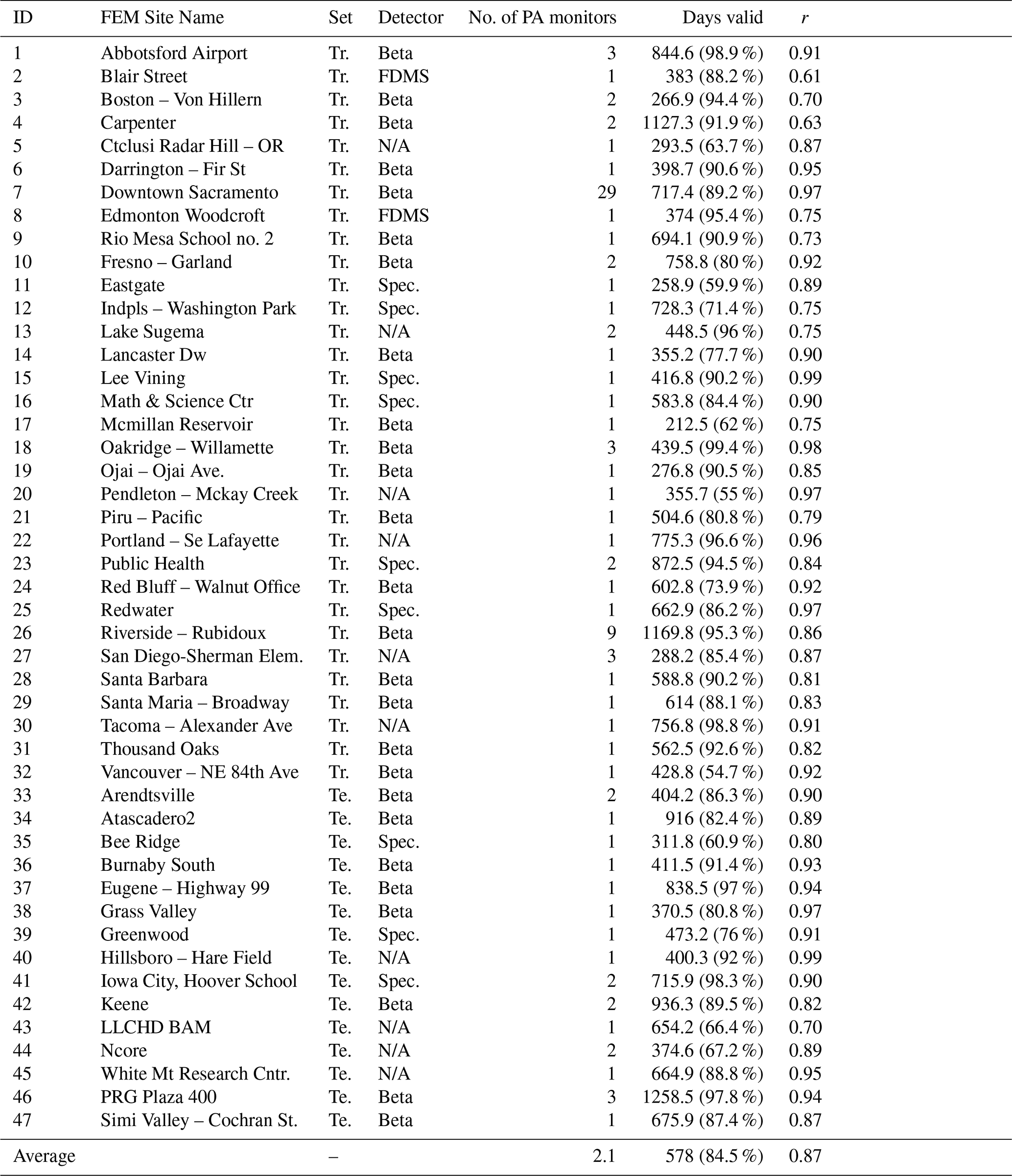
N/A stands for not available.

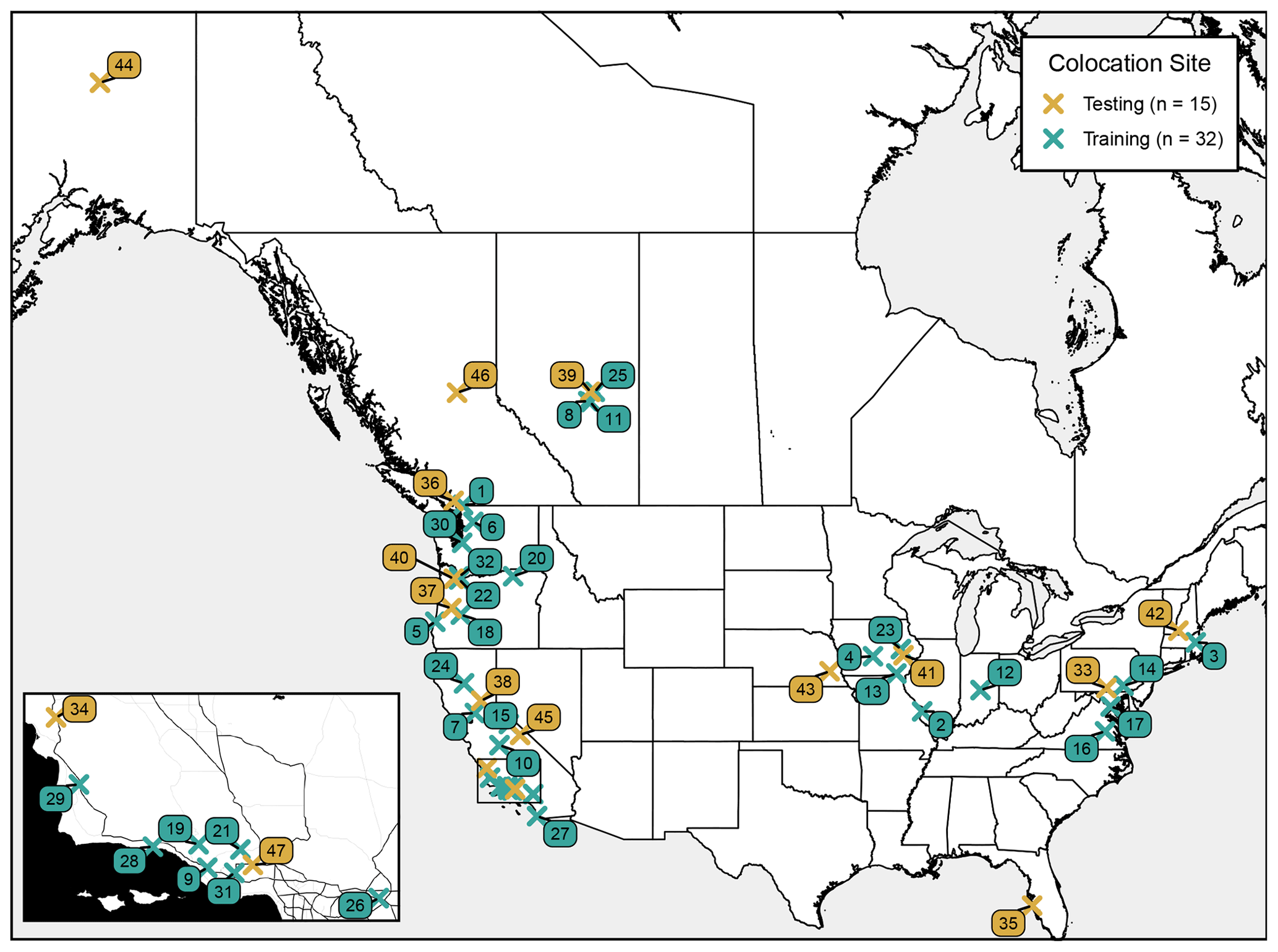
Figure 1 Locations of selected PurpleAir–FEM colocation sites, with numbers corresponding to the ID in Table 1. Of the 47 sites, 32 were used for training the correction models, and the remaining 15 were used for testing. Inset map tiles by Stamen Design, used under CC BY 3.0. © OpenStreetMap contributors 2021. Distributed under the Open Data Commons Open Database License (ODbL) v1.0.

Hourly concentrations of PM_2.5 ranged between 0–837 and 0–986 µg m⁻³ across all sites during this period for PA and FEM monitors, respectively (Fig. 2). PA monitors at most sites tended to be within a factor of 2 of FEM, typically biased higher. For most sites this bias appears to be linear as concentrations increase. PA PM_2.5 concentrations across all sites were categorized as “low AQHI+” (0–30 µg m⁻³) for 91.1 % of observations, “moderate AQHI+” (30–60 µg m⁻³) for 7.7 %, “high AQHI+” (60–100 µg m⁻³) for 0.7 %, and “very high AQHI+” (100+ µg m⁻³) for 0.6 % of observations. For the FEM monitors at all sites, following the order above, 97.5 %, 1.9 %, 0.3 %, and 0.4 % of observations were in the four AQHI+ categories.

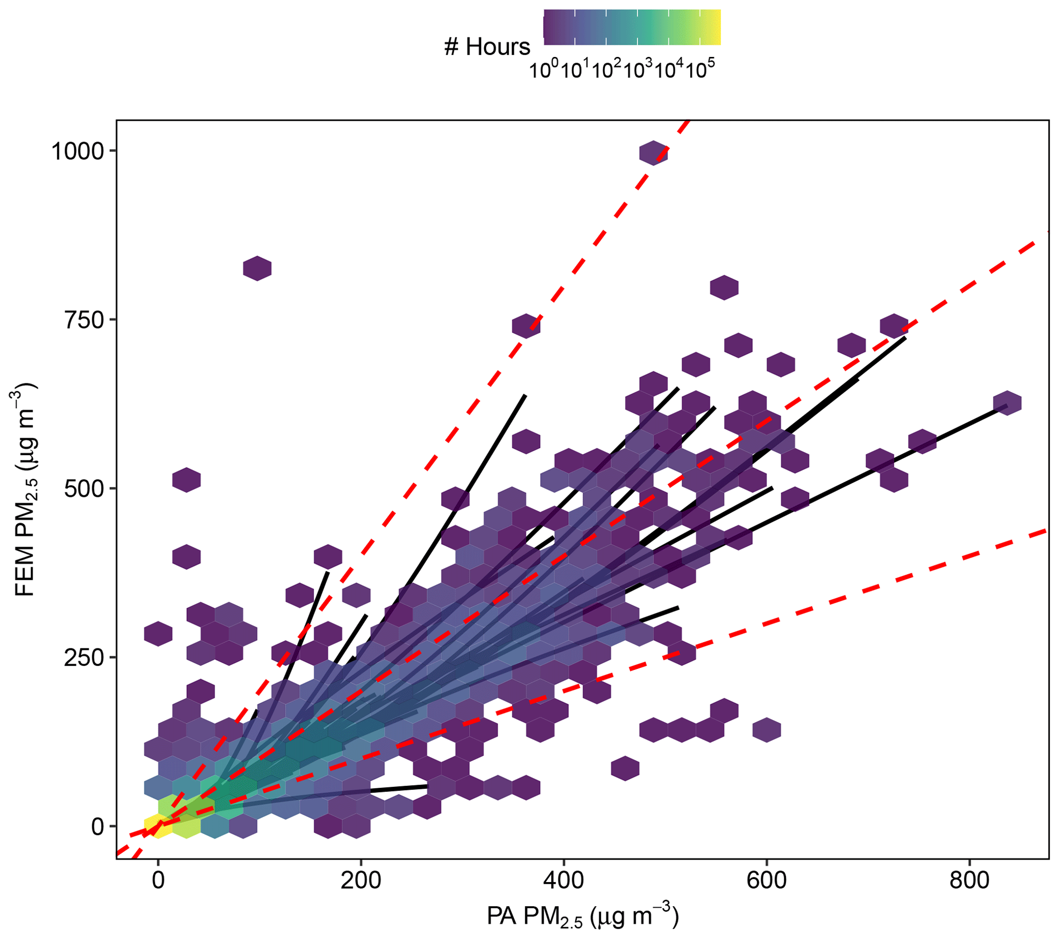
Figure 2 Hourly observation counts of quality-assured and quality-controlled FEM vs. PA PM_2.5 concentrations across all colocation sites in this study. The dashed lines are the 0.5:1, 1:1, and 2:1 lines. The solid lines are individual site general additive models (GAMs), which are chosen over a linear model to provide a general overview of site PA–FEM comparability.

The mean averages of the PA PM_2.5 concentrations at each site tended to be higher than their FEM counterparts in both datasets, except at the lowest humidity levels (Fig. 3). For the training data, 23 % of the hourly observations were classified as “dry” (RH ≤33 %), 56 % were classified as “moderate” (30 % < RH < 70 %), and 21 % were classified as “humid” (RH ≥70 %). The testing data were similar, with 25 %, 55 %, and 19 % of the hours classified as dry, moderate, and humid, respectively. On average, PA concentrations tended to be biased higher as humidity increased; this was not the same case for the FEM monitors which typically have their intake stream heated or dried to lower the RH impacts. Both the FEM and PA monitors had similar ranges of site-median concentrations between the testing and training datasets; however, many of the testing data sites tended to have lower concentrations on average than the training sites.

The FEM monitors in this study utilized one of three main PM_2.5 detection methods (Fig. 4): beta attenuation (26 locations), broadband spectroscopy (9 locations), and FDMS gravimetry (2 locations). There were 10 locations with unknown monitor types (all in the USA). It is most likely that these are beta attenuation monitors based on the high ratio of these detectors in the USA vs. others and the comparability between site mean AQHI+ error shown in Fig. 3; however, some may be broadband spectrometers or gravimetric monitors. There were no significant differences between the mean of the site mean PA AQHI+ errors for each of the FEM sensor types (Kruskal–Wallis p>0.05) when ignoring the FEM observations with an AQHI+ of 1, as these make up the bulk of the observations and are unimportant from a health and management perspective.

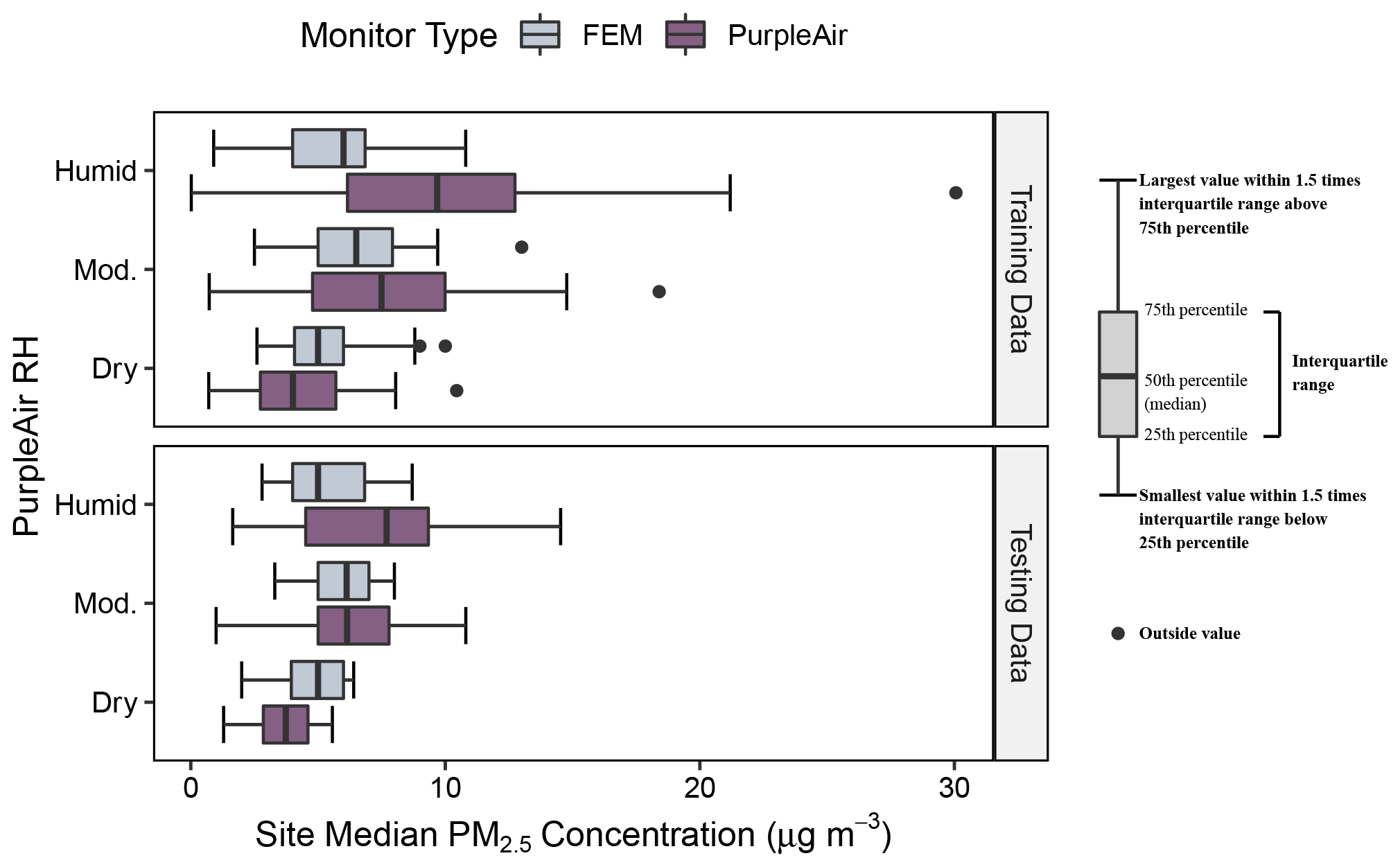
Figure 3 Distributions of the Federal Equivalent Method (FEM) and PurpleAir training and testing sites median PM_2.5 concentrations (µg m⁻³) at dry (0 %–33 %), moderate (34 %–66 %), and humid (67 %–100 %) relative humidity (RH) groupings. The boxplot format is indicated on the right.

Figure 4 Distributions of the site mean PurpleAir AQHI+ error for each of the known FEM detector types. Hours where the Federal Equivalent Method (FEM) AQHI+ was equal to 1 were removed as these make up the bulk of the observations and are unimportant from a health and management perspective. The Kruskal–Wallis global p value (>0.05) is provided in the bottom right, indicating no significant differences between the group means. The boxplot format is the same as in Fig. 3.

3.1 Correction development

Eight correction models were selected for evaluation (Table 2), including four developed in this study from regressing the training data (Models 1–4) and four others available from the literature (Models 5–8). Nearly all of these correction models utilize the “PM_2.5 CF 1” column provided by PA, except Models 6 and 8 which use “PM_2.5 CF ATM”. Model 1 is a multiple linear model including a RH term. Model 2 uses a RH growth adjustment (k=0.24) to reduce the PM_2.5 concentration as RH increases (see Eq. 5). Model 3 is a second-degree polynomial with a RH term included. Model 4 is a three-breakpoint piecewise model with breakpoints selected to visually fit the data best over multiple iterations. The last four equations are provided from studies by other parties and consist of two simple linear models (Models 5 and 6), a multiple linear model including RH (Model 7), and a multiple linear model including both RH and temperature (Model 8).

Table 2 PurpleAir correction models selected for evaluation; pm25_cf1 and pm25_atm are values from the “PM2.5_CF 1” and “PM2.5_CF ATM” columns provided by PA, respectively. The “min” column indicates the minimum corrected value at a RH of 70 %. ^* in the Min column indicates a temperature of 20 ^∘C for Model 8.

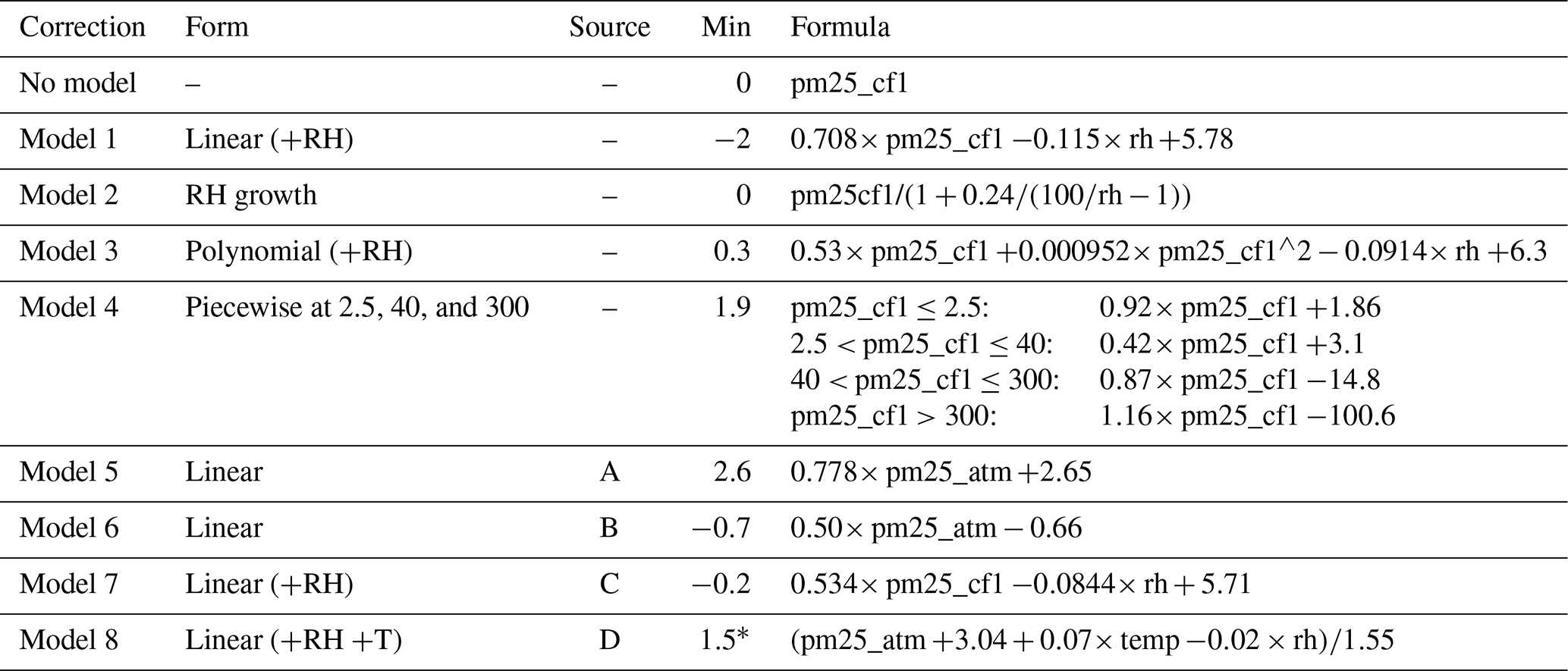
A: Kelly et al. (2017); B: LRAPA (2019); C: Barkjohn et al. (2021); D: Ardon-Dryer et al. (2019).

The corrected data from the models typically had a minimum value of at or just below 0 µg m⁻³, except for Models 4, 5, and 8 which had a higher minimum value (around 2 µg m⁻³). Models 1, 6 and 7 produced negative values during periods of low concentrations and high humidity (which need to be removed or replaced with 0 after correcting). A constant temperature of 20 ^∘C was assumed here for Model 8 to calculate the minimum corrected value.

3.2 Correction evaluation

Raw PA observations were biased positively at FEM AQHI+ levels between 1 and 9, peaking at an AQHI+ of 4 to 7, as shown in Fig. 5. An AQHI+ bias at or near zero is preferred, especially at the higher FEM AQHI+ levels most impactful to human health. Models 2, 5, and 7 minimized this bias the most on average. Model 2 was biased slightly high at AQHI+ of 6 or lower, and slightly high onwards with a minimum at 10 AQHI+. Models 5 and 7 performed similarly; however, they were biased slightly low throughout, except at an AQHI+ of 1, and had the worst performance at 8 and 10 AQHI+. Models 1 and 8 were the next best; however, they were both increasingly negatively biased at higher FEM AQHI+ levels. Model 6 had relatively large negative biases in the 3–10+ AQHI+ levels. A detailed breakdown for each testing site can be found in the Supplement (Fig. S4). Further comparisons were only made on Models 1, 2, 5, and 7 as they showed the best performance here. Comparisons for the remaining models are shown in Fig. S1, Table S1, and Fig. S2.

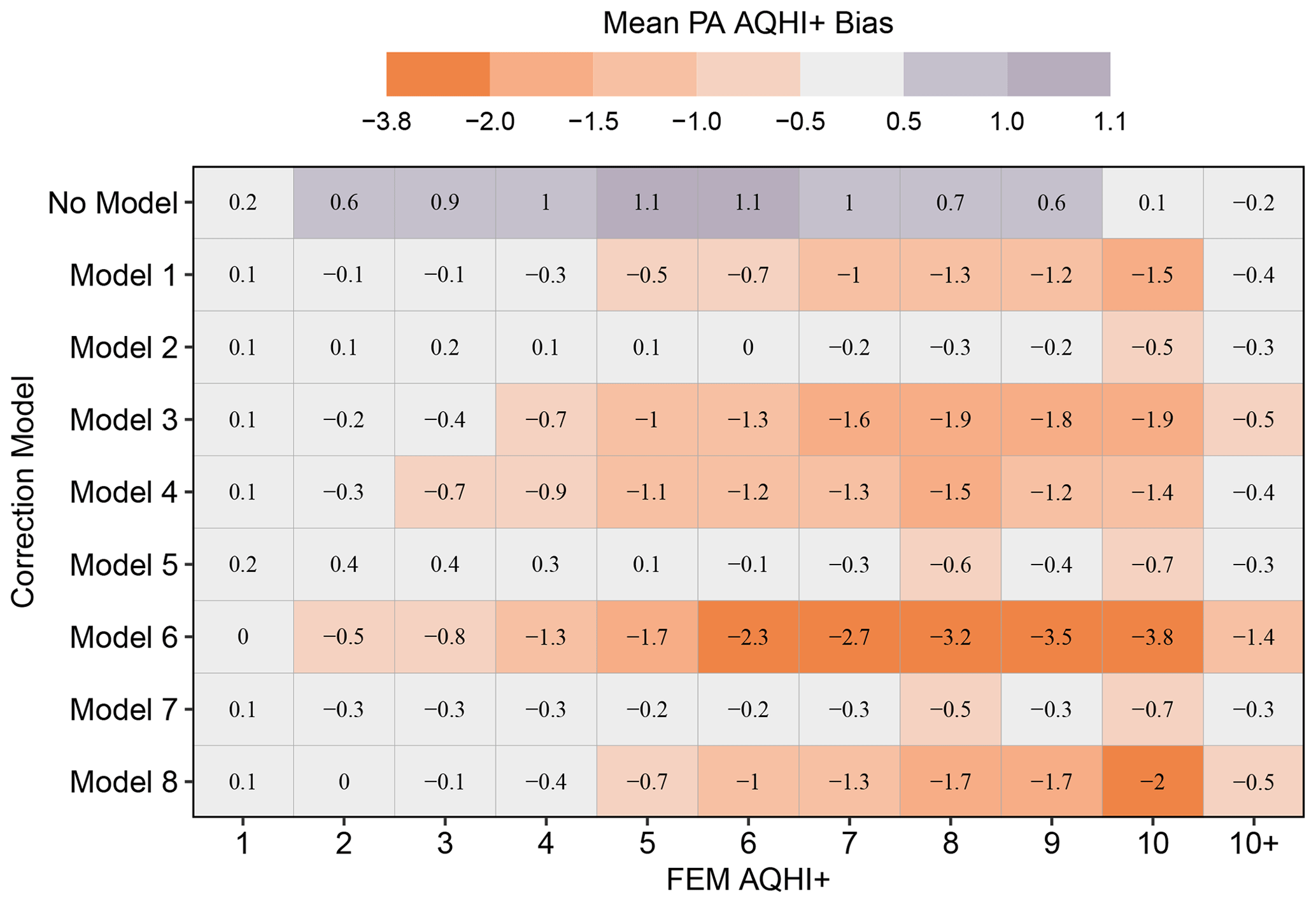
Figure 5 Mean PurpleAir AQHI+ bias for each correction model (including the raw data) at Federal Equivalent Method (FEM) AQHI+ levels. A value at or near 0 is preferred, especially for higher AQHI+.

The NRMSE, NMB, MFE, and MFB for the PA monitors were worse at lower concentrations and improved as concentrations increased (Fig. 6). We saw similar performance between models; all of which improved upon the raw PA observations at most concentrations. Model 1 worsened the MFE and bias measurements in the moderate to high range, Model 5 performed poorly below an AQHI+ of 5, and Models 2 and 7 had the best performance outside of the low-concentration range. Model 7 was best for the very low observations (AQHI+ of 1); however, Model 2 tended to perform better starting at 2–3 AQHI+.

Goal and acceptable levels for MFE and MFB are suggested in Boylan and Russell (2006). Raw PA data meet the goal level of 50 % for all but the lowest AQHI+ for MFE, where it still meets the acceptable level of 75 %. Only Models 7 and 8 bring these lowest concentrations into or near the goal level. Both uncorrected and corrected observations were within the goal range for MFB (±30 %). We assumed goal and acceptable levels for NRMSE of 50 % and 70 %, respectively, to align with the levels defined for MFE. Using these standards, the uncorrected PurpleAir data are unacceptable at AQHI+ equal to 1 and get increasingly better until they reaches the goal level in the high concentrations. Each correction model brings the data into the goal level, except at AQHI+ equal to 1 where it is only acceptable. A goal level of ±30 % was assumed for the NMB as with the MFB and the level defined for mean bias (MB) in Chang and Hanna (2004). Only the uncorrected data for AQHI+ values between 2 and 3 exceeded this goal level across our sites.

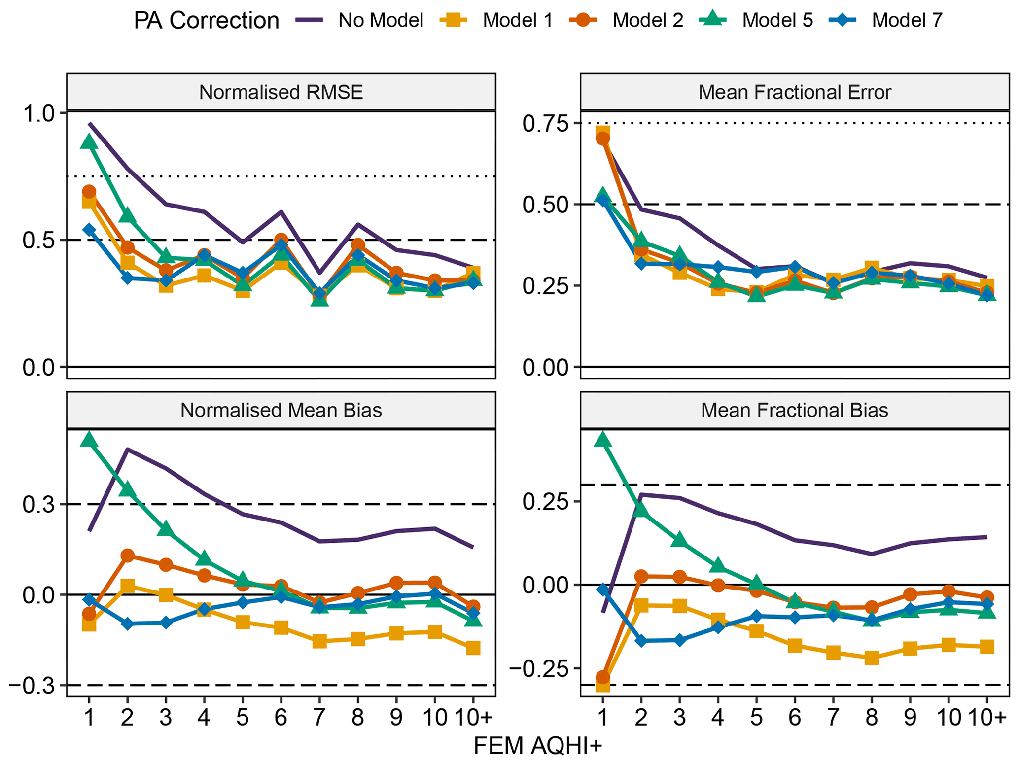
Figure 6 Comparison statistics across Federal Equivalent Method (FEM) AQHI+ levels for select correction models. Goal and acceptable levels are displayed where possible for RMSE (0.75 and 0.5), MFE (0.75 and 0.5), NMB (±0.3 and ±0.6), and MFB (±0.3 and ±0.6).

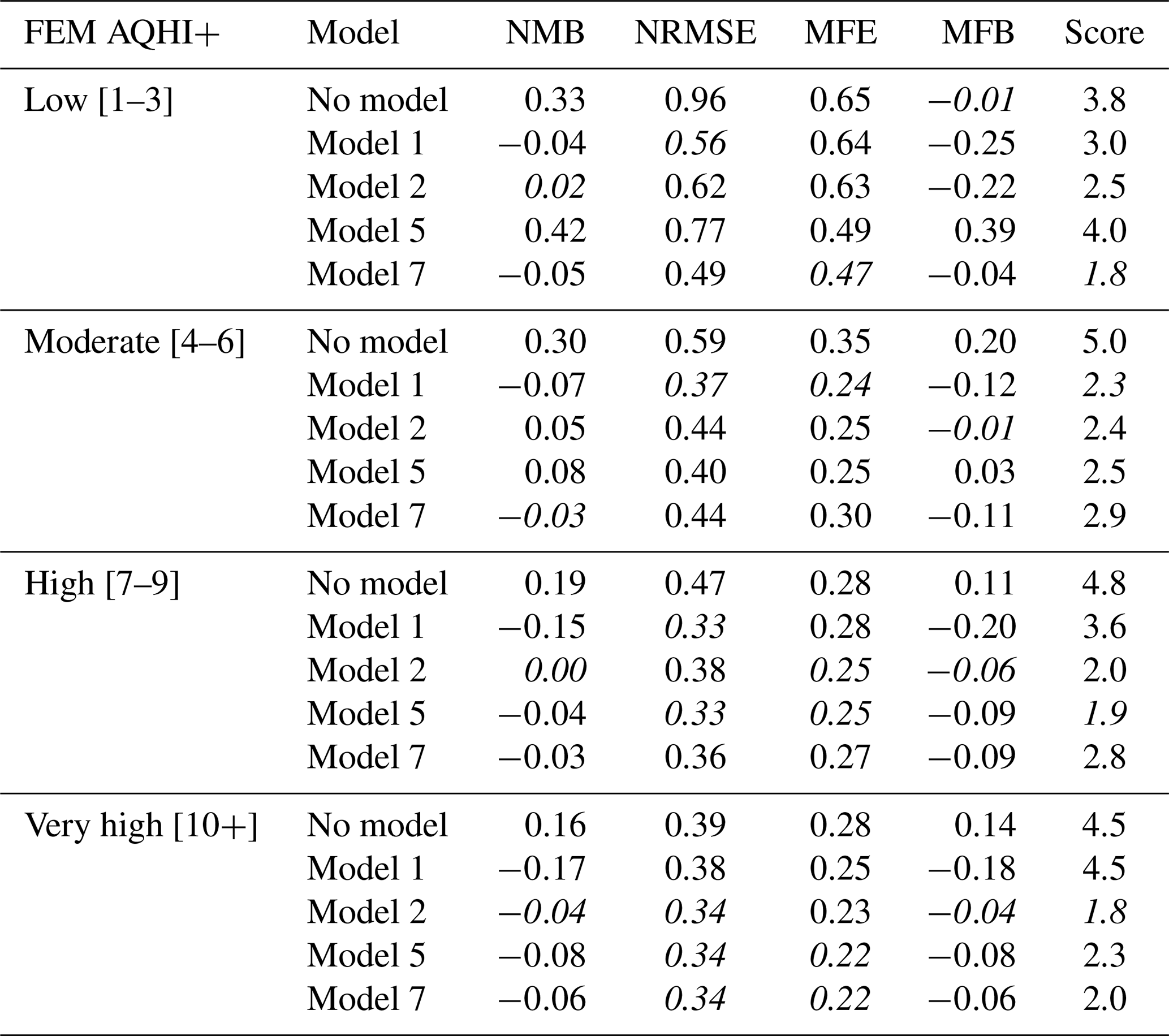
These statistical comparisons were also made on coarser AQHI+ groupings (Table 3). A ranking score was calculated for each model using the mean average of the ranks (from 1 to 5) for each statistic within an AQHI+ group. A lower score indicates better relative performance within that AQHI+ range. Models 2, 5, and 7 performed the best in the high and very high AQHI+ categories. However, the models did not perform as consistently well in the low and moderate ranges. Models 2 and 7 tended to be the best for the low range, while Models 1, 2, and 5 were better for the moderate range.

Table 3 PurpleAir (PA) normalized mean bias (NMB), normalized root-mean-square error (NRMSE), mean fractional error (MFE) and mean fractional bias (MFB) at low, moderate, high, and very high Federal Equivalent Method (FEM) AQHI+ levels for each PA correction model. A crude score is calculated by averaging each statistics integer rank (from 1 to 5) for the models within that AQHI+ group. The top performing models are shown in italics.

The error or bias in AQHI+ from the uncorrected PA monitors was greatest in the moderate to high range (Fig. 7). The selected corrections produced similar improvements to each other, all improving upon the PA's ability to correctly determine the hourly AQHI+ except for at the most extreme concentrations (>100 µg m⁻³). For AQHI+ bias, Model 1 improved upon Model 7, which has the same form, except at very high FEM concentrations. This was not the case for the mean AQHI+ bias; however, as Model 1 becomes increasingly negatively biased as FEM concentrations increase. Model 2 was the best overall performer for both AQHI+ error and bias, being marginally outperformed only in the low-concentration range. This was followed by Models 5 and 7, which performed well except for the mean AQHI+ error in the moderate-concentration range for Model 7.

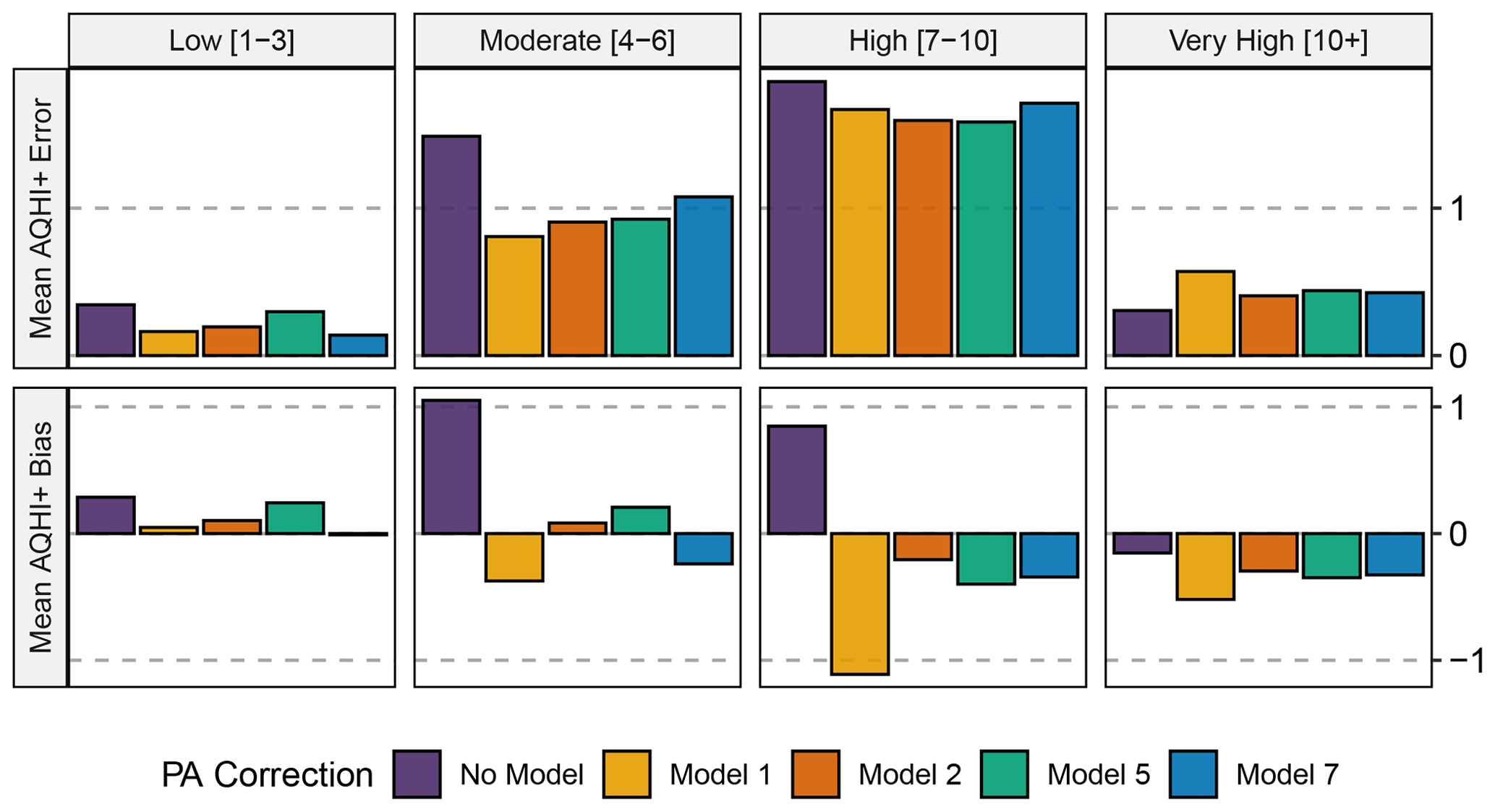
Figure 7 Mean PurpleAir (PA) AQHI+ error and bias for low, moderate, high, and very high Federal Equivalent Method (FEM) AQHI+ levels for selected correction models.

Model 2 produces a mean AQHI+ bias and error consistently closer to 0 than the other correction models (or no model at all) across the range of observed concentrations. Only at the lowest concentrations do the other models marginally outperform Model 2 across our testing sites for most of the comparisons made.

4 Conclusions

The concentrations of PM_2.5 reported from the PA monitors were biased high compared to the FEM monitors at most colocation sites, especially for the lower-concentration range. This bias is attributed to both the method of detection as well as hygroscopic growth from increased humidity. No significant differences were detected between FEM sensor methods, which are rigorously tested and evaluated to ensure this consistency. Based on our colocation method there is a risk that some sites are not true colocation sites; however, given the proximity of the monitors and good correlation (>60 %), we decided the potential impact would be minimal. The Canadian AQHI+ system was useful as a framework for evaluating correction models across a range of concentrations, as infrequent high values or numerous low values can skew performance statistics when evaluating the full range at once.

The selected corrections discussed here improve the performance of PA similarly; however, Model 2 (our “RH Growth” model) had consistently better performance, especially at moderate to high concentrations that are important to health. This was followed closely by Model 7, the multiple (RH) linear regression from Barkjohn et al. (2021), and Model 5, the simple linear regression from Kelly et al. (2017). Model 1, our multiple linear regression with the same form as Model 7, performed well in the low to moderate range; however, it did not perform as well at higher concentrations. It should be noted that the average performance across the testing sites and over time was evaluated here; performance at colocation sites and across time was not the same (see Fig. S4). In addition, while our correction model focuses on correcting the impacts of humidity, other characteristics like refractive index and particle shape, density, and size distribution may account for differences in PM_2.5 estimates.

Future studies should focus on developing and evaluating correction models as more data become available from the PA network, as well as installing and documenting additional colocation sites. Specifically, the k value utilized in our Model 2 should be adjusted and re-evaluated as more collocation data become available. Valid collocation data are imperative for both developing and evaluating low-cost monitor performance before and after applying a correction formula. These corrections should be evaluated in comparison with the others available to ensure comparable or improved performance.

We recommend testing the performance of several models at specific sites of interest and selecting the best-performing model for a given site (Fig. S4 provides a breakdown for the testing sites and models evaluated here). Models 1, 2, 5, and 7 presented here are good starting points. As more colocation data become available, seasonal and area-specific correction models should be examined. Performance in the moderate- to high-concentration range should be focused on as these are the most important from a health perspective; the low concentrations are less important, while also being the most observed levels in the US and Canada. Correlation is useful for evaluating overall monitor performance at a site, but not as useful for evaluating and comparing correction performance. Normalized methods such as NRMSE, MFB, or MFE are good measures, but we recommend evaluations across a range of PM_2.5 concentrations, such as using the AQHI+ framework as presented here. If one intends to develop a site-specific correction model, we recommend using the same form as our Model 2 while adjusting the k value. For scenarios where testing models on individual locations is not an option, such as applying a correction in an area without a nearby PA–FEM colocation site, we recommend using our Model 2.