Use of large-eddy simulations to design an adaptive sampling strategy to assess cumulus cloud heterogeneities by remotely piloted aircraft

Trade wind cumulus clouds have a significant impact on the Earth's radiative balance due to their ubiquitous presence and significant coverage in subtropical regions. Many numerical studies and field campaigns have focused on better understanding the thermodynamic, microphysical, and macroscopic properties of cumulus clouds with ground-based and satellite remote sensing as well as in situ observations. Aircraft flights have provided a significant contribution, but their resolution remains limited by rectilinear transects and fragmented temporal data for individual clouds. To provide a higher spatial and temporal resolution, remotely piloted aircraft (RPA) can now be employed for direct observations using numerous technological advances to map the microphysical cloud structure and to study entrainment mixing. In fact, the numerical representation of mixing processes between a cloud and the surrounding air has been a key issue in model parameterizations for decades. To better study these mixing processes as well as their impacts on cloud microphysical properties, the paper aims to improve exploration strategies that can be implemented by a fleet of RPA.

Here, we use a large-eddy simulation (LES) of shallow maritime cumulus clouds to design adaptive sampling strategies. An implementation of the RPA flight simulator within high-frequency LES outputs (every 5 s) allows tracking individual clouds. A rosette sampling strategy is used to explore clouds of different sizes that are static in time and space. The adaptive sampling carried out by these explorations is optimized using one or two RPA and with or without Gaussian process regression (GPR) mapping by comparing the results obtained with those of a reference simulation, in particular the total liquid water content (LWC) and the LWC distribution in a horizontal cross section. Also, a sensitivity test of length scale for GPR mapping is performed. The results of exploring a static cloud are then extended to a dynamic case of a cloud evolving with time to assess the application of this exploration strategy to study the evolution of cloud heterogeneities. While a single RPA coupled to GPR mapping remains insufficient to accurately reconstruct individual clouds, two RPA with GPR mapping adequately characterize cloud heterogeneities on scales small enough to quantify the variability of important parameters such as total LWC.

1 Introduction

Cumulus clouds are ubiquitous over the subtropical oceans and cover more than 20 % of the ocean surface on average (Eastman et al., 2011). They mainly interact with shortwave radiation and therefore exert a net cooling effect on the Earth system. They also modulate the water and energy cycles of the atmosphere through vertical transfer from the sub-cloud layer to the cloud layer. Cumulus clouds are therefore a key element of the climate system (Park et al., 2017). Their representation in global circulation models (GCMs) has been shown to be responsible for large uncertainties in the climate response (Andrews et al., 2012). Due to their grid scales between 10 and 100 km, GCMs cannot explicitly represent shallow clouds and use parameterizations to represent the impacts of such clouds on the climate radiation budget. One of the biggest uncertainties in understanding the impacts of cumulus clouds on the water and energy cycle is related to mixing processes (Sanchez et al., 2020). Mixing processes and entrainment impact cloud microphysical properties by creating heterogeneities of thermodynamical variables, diluting the liquid water content, and reducing the cloud albedo. Studies on these processes often rely on the analysis of large-eddy simulations (LESs) that reproduce average properties of shallow convection (Guichard and Couvreux, 2017; Siebesma and Jonker, 2000; Neggers et al., 2003; Heus and Jonker, 2008). However, such models, with a horizontal resolution of a few tens of meters, still use parameterizations to represent cloud microphysics and small-scale turbulence to correctly reproduce sub-grid heterogeneities inside cumulus clouds such as sub-grid-scale liquid water content (LWC) variability resulting from mixing processes at the cloud–air interface.

Observations of cumulus horizontal structures in the western Atlantic Ocean have been obtained from field campaigns such as BOMEX (Barbados Oceanographic and Meteorological EXperiment, Holland and Rasmusson, 1973), SCMS (Burnet and Brenguier, 2007), CARRIBA (Siebert et al., 2013), and RICO (Rauber et al., 2007), and cloud instrumentation continues to improve (e.g., the Fast-FSSP, Brenguier et al., 1998; and the HOLODEC – Holographic Detector for Clouds, Fugal and Shaw, 2009). However, a sampling strategy that relies on one or two transects through the same cloud only is not sufficient to reconstruct the cloud cross section or follow its evolution. Observations from research aircraft such as Burnet and Brenguier (2007) or with sensors suspended under a helicopter (Siebert et al., 2006; Katzwinkel et al., 2014) have conducted multiple transects through an individual cloud with a lower frequency (a maximum of five transects). It has been shown that airplane transects without cloud mapping induce a bias in cloud sampling by oversampling the cloud core (Hoffmann et al., 2014). In addition, this paper illustrates the importance of extending the transects with Gaussian process regression (GPR) mapping to capture the fractal nature of clouds.

The field campaigns serve as a basis for the construction of well-established case studies in which LESs have been used to develop and evaluate shallow cloud parameterization (Siebesma et al., 2003; vanZanten et al., 2011). The LESs reproduce the cloud field and allow the study of isolated clouds in detail, notably at high spatial and temporal resolution (Zhao and Austin, 2005a).

Over the past 2 decades, remotely piloted aircraft (RPA) have emerged as a viable tool for observing aerosols and clouds (Roberts et al., 2008; Sanchez et al., 2017; Calmer et al., 2019). Their ability to operate as a fleet and follow complex trajectories based on adaptive sampling is an asset which allows a detailed comparison with high-resolution simulations. Previous studies have developed tools to implement RPA in LESs to optimize trajectories within the cloud environment with the objective to maximize information gain while minimizing energy consumption (Reymann et al., 2018). In this study, we focus on obtaining relevant meteorological data to observe cloud heterogeneities and mixing. A powerful tool in RPA cloud tracking is Gaussian process regression (GPR) mapping during flights to best guide the RPA pattern and during post-processing to reconstruct the cumulus field (Renzaglia et al., 2016).

The objective of this study is to simulate RPA flights in LES output in order to optimize an adaptive sampling strategy to provide sufficient thermodynamic information within a maritime cumulus cloud to quantify the mixing processes. This study is part of the NEPHELAE project (Network for studying Entrainment and microPHysics of cLouds using Adaptive Exploration), which aims to design and develop an automated fleet of RPA to track a cloud from the beginning to the end of its life cycle. Section 2 presents the LES model, cloud identification methods, and the details of the RPA flight parameters. Section 3 highlights the results of the LES case study with a description of the cumulus field. We first classify individual simulated clouds into three categories based on their volume. We then select one cloud representative of each category and analyze the evolution of their macrophysical and thermodynamical properties where the adaptive exploration strategy is applied. Different parameters related to the number of RPA and the use of mapping are compared in a static case to reconstruct macrophysical and thermodynamic fields. The last section focuses on the application of the exploration in dynamics and the associated limitations.

This study highlights benefits of adaptive sampling and GPR mapping and illustrates the potential of RPA to address long-standing challenges in observing clouds.

2 Methodology

2.1 Cloud simulation

2.1.1 BOMEX: a case of marine convection

The numerical simulations focus on the period of 22–23 June 1969 of phase 3 of the BOMEX campaign. These days are characterized by the presence of a strong inversion at the top of the boundary layer (Siebesma and Cuijpers, 1995). This case has been chosen because it represents a typical undisturbed non-precipitating trade cumulus cloud field.

The BOMEX case was the subject of a model intercomparison exercise (Siebesma et al., 2003) with 10 LESs based on different models. The LESs all start with the same initial profiles of total mixing water ratio (q_t) and liquid potential temperature (θ_l) from sea level to the boundary layer top measured by radiosondes. These LES models use prescribed constant surface latent and sensible heat fluxes of 8×10³ K m s⁻¹ and $\mathrm{5.2}\times {\mathrm{10}}^{-\mathrm{5}}$ K m s⁻¹ as well as prescribed large-scale and radiative forcing (Siebesma and Cuijpers, 1995). These LESs also correctly reproduced the observed vertical thermodynamical structure and turbulent fluxes for this period (Nitta and Esbensen, 1974). The horizontal winds are initialized with U=8.75 m s⁻¹ and V=0 m s⁻¹ between sea level and 700 m a.s.l. (meters above sea level) and decrease linearly until $U=-\mathrm{4.61}$ m s⁻¹ at 3000 m a.s.l.

2.1.2 Meso-NH model and configuration

Meso-NH, a French non-hydrostatic mesoscale atmospheric model (Lac et al., 2018), is used in LES mode to simulate the BOMEX case and the results are compared to the LES intercomparison of Siebesma et al. (2003) in Sect. 3. The classical configuration for LES (detailed in Lac et al., 2018) is used here. Lateral boundary conditions are cyclic, and a damping layer is applied at the top of the domain to prevent the reflection of gravity waves. The three-dimensional turbulence scheme from Cuxart et al. (2000) is based on a prognostic equation for the sub-grid turbulence kinetic energy with a Deardorff mixing length (Deardorff, 1980). Trade cumuli contain only liquid water, and aerosol spectra are not available from the BOMEX campaign to initialize a two-moment microphysical scheme; therefore, only a warm bulk one-moment microphysical scheme is used. Longwave radiative cooling, corresponding to the effect of clear-sky emissions, is prescribed for each atmospheric column as a temperature tendency. A saturation adjustment scheme is used, so the grid is either entirely saturated (cloud) or entirely clear (no cloud).

The BOMEX case (Siebesma et al., 2003) was re-simulated for this study using Meso-NH LES with $\mathrm{\Delta }x=\mathrm{\Delta }y=\mathrm{\Delta }z=\mathrm{25}$ m – a higher horizontal resolution than used for the intercomparison study ($\mathrm{\Delta }x=\mathrm{\Delta }y=\mathrm{100}$ m, Δz=40 m; Siebesma and Cuijpers, 1995; Siebesma et al., 2003). The Meso-NH LES was conducted on two different horizontal domains: the same domain as the intercomparison study ($\mathrm{6.4}\mathrm{km}\times \mathrm{6.4}\mathrm{km}\times \mathrm{4}\mathrm{km}$ with $\mathrm{256}\times \mathrm{256}\times \mathrm{160}$ grid points) named 6.4 km_MNH and a domain 4 times larger ($\mathrm{12.8}\mathrm{km}\times \mathrm{12.8}\mathrm{km}\times \mathrm{4}\mathrm{km}$ with $\mathrm{512}\times \mathrm{512}\times \mathrm{160}$ grid points) named 12.8 km_MNH. The radiative tendency was prescribed for each hour following the values presented in Siebesma et al. (2003). The duration of these simulations is 6 h; the first 2 h of the simulation are discarded as spin-up. The 12.8 km_MNH run continued for 30 min longer during which 3D fields were stored every 5 s in order to have high-resolution data on cloud fields, named HFS for high-frequency sampling.

2.1.3 LES validation

To validate the high-resolution Meso-NH, the total cloud cover (TCC) is compared to results from the reference intercomparison study (Siebesma et al., 2003) as shown in Fig. 1. The TCC and liquid water path (LWP) stabilize after the spin-up (20 min delay in Meso-NH; however, convection results in a similar intensity) to ∼15 % and ∼5 g m⁻², respectively. From the second to the sixth hour, the TCC of both Meso-NH simulations remains within the standard deviation of the intercomparison study (Siebesma et al., 2003) with more fluctuations for the 6.4 km domain.

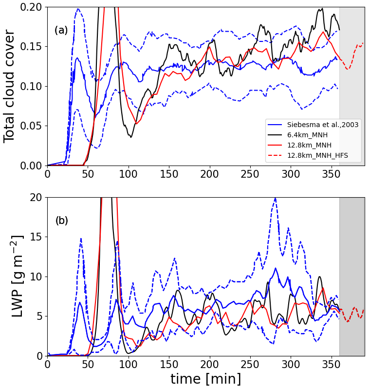
Figure 1 Temporal evolution of (a) total cloud cover and (b) liquid water path from the Siebesma et al. (2003) intercomparison (blue lines; solid line for the mean and dotted line for the ± standard deviation). The black line is for the 6.4 km_MNH domain and the red line for the 12.8 km_MNH domain. Gray shaded area corresponds to Meso-NH high-frequency outputs (HFS).

At the end of the simulation, TCC from 6.4 km_MNH is slightly higher (+5 %) than reported in Siebesma et al. (2003), while LWP remains nearly the same, confirming the study of Matheou et al. (2011), who argued that a better spatial resolution significantly increases the TCC.

The vertical profiles of turbulent flux of q_t, θ_l, wind, turbulent kinetic energy (TKE), and LWC are also near the mean and within the variability of the intercomparison ensemble presented in Siebesma et al. (2003) (not shown). The TCC in HFS (shaded area in Fig. 1) varies between 11.9 % and 15.3 % during the 30 min, while the mean LWP in the domain is between 4.30 and 6.07 g m⁻². In the following sections, the analysis focuses on the high-temporal-frequency outputs (HFS) in order to study the life cycle of individual clouds.

2.1.4 Cloud identification method

One of the main objectives is to be able to characterize an entire cloud life cycle, including the formation phase when updrafts dominate and the dissipation phase when downdrafts dominate. In order to do that, we need to track individual clouds as a function of time while exploiting the high spatial and temporal resolution of the LES.

We first define clouds as coherent 3D structures made of at least eight contiguous cells containing LWC $>\mathrm{1}\times {\mathrm{10}}^{-\mathrm{3}}$ g kg⁻¹ and overlapping for at least two vertical levels; i.e., clouds thinner than 50 m or smaller than $\mathrm{1.25}\times {\mathrm{10}}^{-\mathrm{4}}$ km³ are filtered out. In order to follow individual clouds, we apply a method of cloud identification (Brient et al., 2019) as a function of time, t. As shown in Fig. 2, the cloud identification method uses matrices of contiguity that isolate a cell and define it as belonging to cloud N. For each cloudy cell, the method identifies the neighboring cells connecting by their face, edge, or corner. If one of them is already tagged as a cloudy cell, it will get the same tag (Fig. 2, t₀). This method also uses contiguity in time, with the criterion that a face, an edge, or a corner of a cloudy cell at t_n touches a cloudy cell at t_n−1 (Fig. 2, t₁). However, the advection of the cloud must be within a spatial limit between two time steps defined by the Courant–Friedrichs–Lewy condition (CFL $=(U\mathrm{\Delta }t/\mathrm{\Delta }x)\le \mathrm{1}$). If the cloud moves two or more lengths during one time step, the cloud identification method can lead to errors. In this study, the advection wind U is between 5 and 8 m s⁻¹, the horizontal resolution is Δx=25 m, and outputs are produced every 5 s, which yields a CFL between 1 and 1.6 and does not meet the CFL condition. To solve this issue, only cumuli with an overall dimension at least 3 times larger than a mesh (cloud width ≥75 m) are identified. When filtering small clouds out, the TCC and LWP do not change significantly (less than −0.05 % and $-\mathrm{6}\times {\mathrm{10}}^{-\mathrm{3}}$ g m⁻³, respectively). A newly condensed cell can be added to the edge of the cloud, linked to a previous cloud cell (Fig. 2, t₂), or identified as a new cloud (Fig. 2, t₃). The strength of this cloud identification method is that it can identify individual clouds in the model domain quickly.

Figure 2 Scheme of temporal cloud identification method for following a cloud in a dynamic environment.

2.2 Description of observational strategy

To improve upon decades of cloud observations, there is a need to follow a cloud throughout its life cycle and determine, with high spatial and temporal resolution, its microphysical and thermodynamical properties. The goal of this study is to derive the best strategy to observe the evolution of an individual cloud. The flight strategy ultimately depends on how long it takes to sample the cloud, which is largely determined by the RPA air speed to transect the cloud and its turning radius to turn around and re-enter the cloud. In these simulations, the RPA samples every grid point along its transect. Simulations in this study were conducted using an RPA air speed of 15 m s⁻¹ and a turning radius of 100 m (Verdu et al., 2019). In order to optimize the sampling of clouds by the RPA, a rosette flight pattern is performed in the LES to create a horizontal cross section of the cloud. The flight simulation is controlled by the Paparazzi autopilot module (Hattenberger et al., 2014), which makes it possible to simulate the behavior of an RPA within the LES. The autopilot module and the LES are combined with the module CAMS (Cloud Adaptive Mapping System). The payload module, which simulates a cloud instrument, is embedded in the Paparazzi autopilot module to detect the presence of a cloud using a threshold of LWC $\ge {\mathrm{10}}^{-\mathrm{2}}$ g m⁻³. If the LWC threshold is exceeded, the RPA begins its rosette pattern by conducting a straight line until it exits the cloud. The geometric center (red point in Fig. 3, t₀) is calculated using a weighted sum of the LWC after each passage through a cloud. After exiting the cloud (LWC $\le {\mathrm{10}}^{-\mathrm{2}}$ g m⁻³), the RPA turns back toward the cloud center (Fig. 3, t₁), and the transects are repeated in the form of a rosette pattern until the cloud disappears.

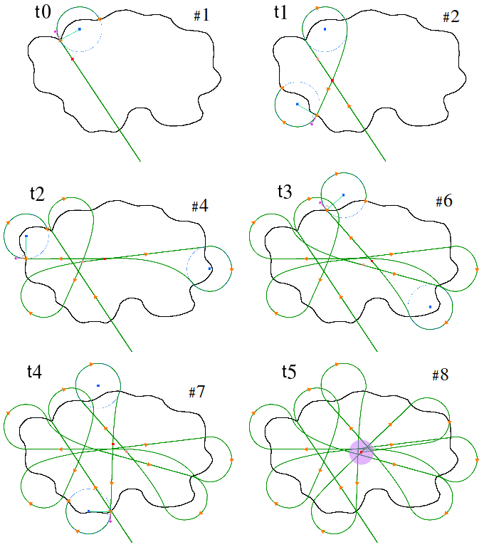
Figure 3 Rosette pattern for different times (and the number of transect associated) of exploration; adapted from Verdu et al. (2019). Green lines represent the RPA trajectories, red points the calculated geometric center at different times of exploration, and the purple point the last geometric center.

3 Results

This section exploits the high temporal and spatial resolution provided by the LES to optimize the adaptive sampling for static and dynamic cases. First, an overview of the different clouds sampled in the LES is provided before selecting three clouds representative of the cloud population. Then, an exploration of the selected clouds is carried out with RPA flying offline in the simulations – first in a static mode (i.e., without taking into account the displacement of the cloud) and then in a dynamic mode (i.e., including the wind advection and time evolution of the cloud).

3.1 Description of a simulated trade cumulus field

During the HFS (12.8 km_MNH domain), an average of 300 clouds per output are identified with a minimum of 270 clouds around the 18th minute and a maximum of 350 clouds at the 25th minute (Fig. 4). Individual cloud volumes have been separated into four classes. Class 0 corresponds to a volume between 10⁻⁴ and 10⁻³ km³, class 1 between 10⁻³ and 10⁻² km³, class 2 between 10⁻² and 10⁻¹ km³, and class 3 between 10⁻¹ and 1 km³ (Table 1). Figure 4 presents the evolution of the number of clouds detected at each time step (every 5 s). The volume distribution shows that one-third of the clouds are in class 0, another third in class 1, and another third in class 2 and 3 with just under 10 clouds exceeding 10⁻¹ km³ at any given time. The temporal evolution in Fig. 4 of the different classes shows a certain stability in the cloud field. Despite the small number of clouds classified in class 3, they have a disproportionate role in the transport of moisture and heat in the boundary layer since their mass flux is more than an order of magnitude larger than the clouds of classes 0 and 1.

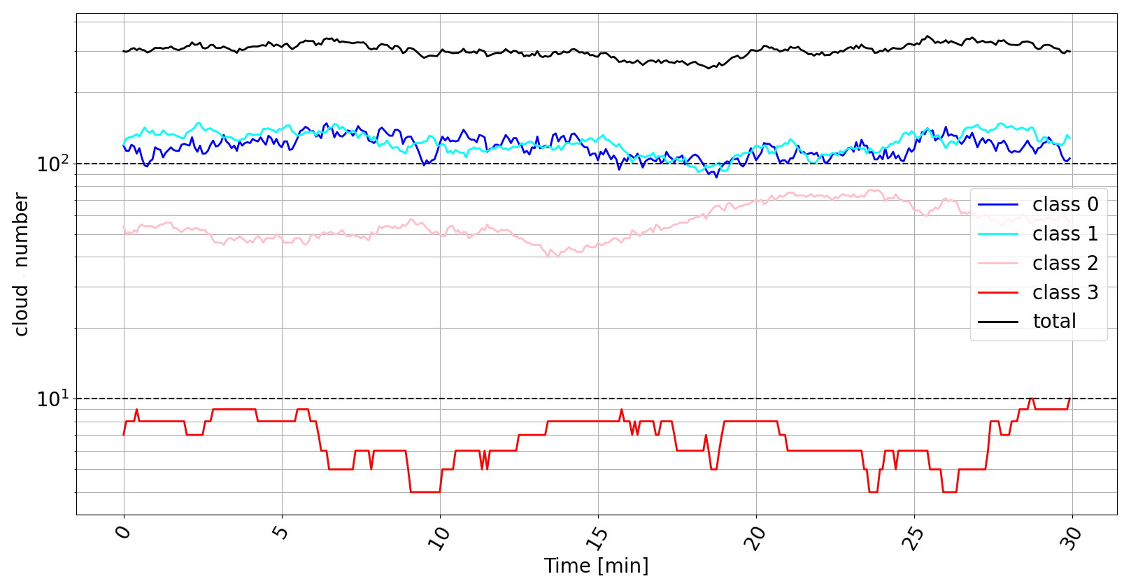
Figure 4 Temporal evolution of the number of clouds at each model output classified by their different volumes from Table 1.

Table 1 Min, max, mean, and standard deviation of macroscopic and dynamic characteristics of the 970 clouds that complete a full life cycle during HFS.

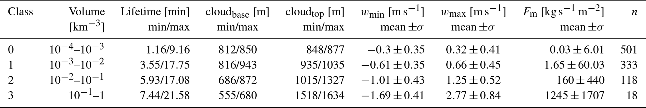
Some 2150 independent clouds have been identified, 970 of which complete a full life cycle within the 30 min HFS. For clouds with the life cycle fully described from formation to dissipation, statistics are calculated for thermodynamical and macrophysical properties for each of the four volume classes, as shown in Table 1. For each class, the minimum (maximum) lifetime is calculated by averaging the smallest (largest) 10th percentile, and the minimum cloud base height (cloud-top height) is calculated by averaging all the minimum cloud base heights (cloud-top heights) of each cloud during their lifetime. The cloud base of a newly formed cloud is always at the level of the lifting condensation level (LCL), which is around 550 m a.s.l. The larger the volume, the lower the average cloud base (which ranged between 550–680 m), and inversely, the smaller the volume, the higher the average cloud base (around 800 m). The cloud base also tends to increase when the cloud dissipates, which increases the average cloud base, particularly for small clouds. The lifetime of small clouds is notably less as they dissipate quickly. The height of the cloud top also increases with the volume, as vertical extension is larger than the horizontal extension for cumulus clouds (Neggers et al., 2003). The larger the volume, the greater the intensity of the downdrafts w_min and updrafts w_max. To calculate w_min and w_max, the highest downdraft and updraft are selected in each individual cloud during its lifetime and then averaged per class. The maximum downdrafts and updrafts in this study are observed in the biggest clouds (class 3; −1.69 and 2.77 m s⁻¹).

The average mass flux of the clouds (F_m) is positive, but the standard deviation is larger than the mean in all four classes. Standard deviations of mass flux indicate that variability is related to formation, dissipation, and width of the bin. A negative F_m represents the dissipation of the cloud and occurs more often for small clouds than large clouds. The difference in magnitude value of F_m between the size classes is significant, with an order of magnitude of difference in F_m for an order of magnitude change in cloud volume.

3.2 Individual cloud description

Inspired by the study of Zhao and Austin (2005a), who use an LES with a similar resolution ($\mathrm{\Delta }x=\mathrm{\Delta }y=\mathrm{\Delta }z=\mathrm{25}$ m) to study thermodynamical processes in individual clouds with volumes of 10⁻² and 10⁻¹ km³, this study focuses on three independent clouds representative of volumes of 10⁻² km³ (N1, class 1), $\mathrm{2}\times {\mathrm{10}}^{-\mathrm{2}}$ to $\mathrm{3}\times {\mathrm{10}}^{-\mathrm{2}}$ km³ (N2, class 2), and 10⁻¹ km³ (N3, class 3).

3.2.1 Macrophysical and microphysical properties

The evolution of the life cycle for the three clouds (N1, N2, N3) is followed for 12, 18, and 24 min, respectively. The growing phase, corresponding to an increase in volume, comprises 55 %–65 % of their life cycle. Each of the clouds has a similar cloud-base height (at 550 m), and their cloud-top increase follows a logarithmic growth rate, with a higher rate for large clouds. The maximum surface of the horizontal cross section at 150 m above cloud base occurs at t=14 min for cloud N1 with S_max=0.045 km², t=10 min for cloud N2 with S_max=0.28 km², and t=15 min for cloud N3 with S_max=1.06 km². In Fig. 5c, the maximum LWC for the three clouds is compared to their pseudo-adiabatic profile, computed by integrating the adiabatic vertical gradient, β, through the cloud depth (Korolev, 1993). The difference between pseudo-adiabatic and maximum LWC for each cloud level indicates the degree of entrainment mixing that has occurred. The maximum LWC in the HFS follows the pseudo-adiabatic profile to approximately a third of the height of the clouds. The LWC then remains more or less constant until decreasing near the top, suggesting higher entrainment rates in the upper part of the clouds.

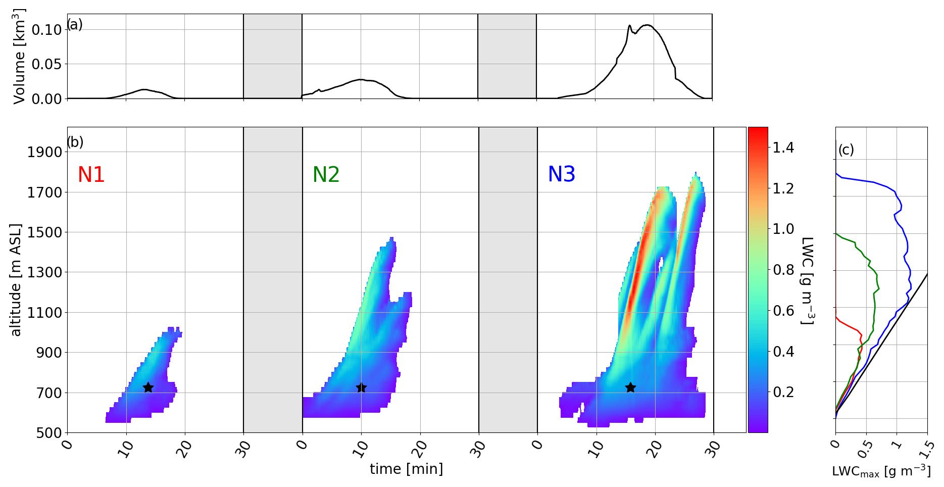
Figure 5 Life cycle of three clouds N1, N2, and N3 for (a) their volume and (b) their LWC. The black star represents altitude and time for static cloud exploration. (c) The comparison between the maximum LWC for each vertical level during each cloud life cycle and the limit of pseudo-adiabatic LWC (black line).

3.2.2 Thermodynamical properties

Consistent with Zhao and Austin (2005b) and Heus et al. (2009), the clouds in the HFS present single or several pulses. As shown in Figs. 5 and 6, cloud N1 can be described by a simple pulse growth, whereas clouds N2 and N3 show two and three pulses, with the first being the most important. The maximum updraft occurs at maximum volume and at the top of each pulse when the cloud has reached its mature phase, while maximum downdraft remains relatively constant (Fig. 6a). Similar features are seen for clouds N1, N2, and N3, for which the magnitude of the updrafts and downdrafts is related to the size of the cloud (Table 1). Figure 6b represents the time series of the mean vertical mass flux for each cross section. High values of vertical mass flux are located near cloud base and within the cloud core (studied for each cloud cross section), and they remain nearly constant up to half the height of the cloud, while negative vertical mass fluxes are always located near the cloud edge (also studied for each cloud cross section) and cloud top in the dissipation phase (Fig. 6c).

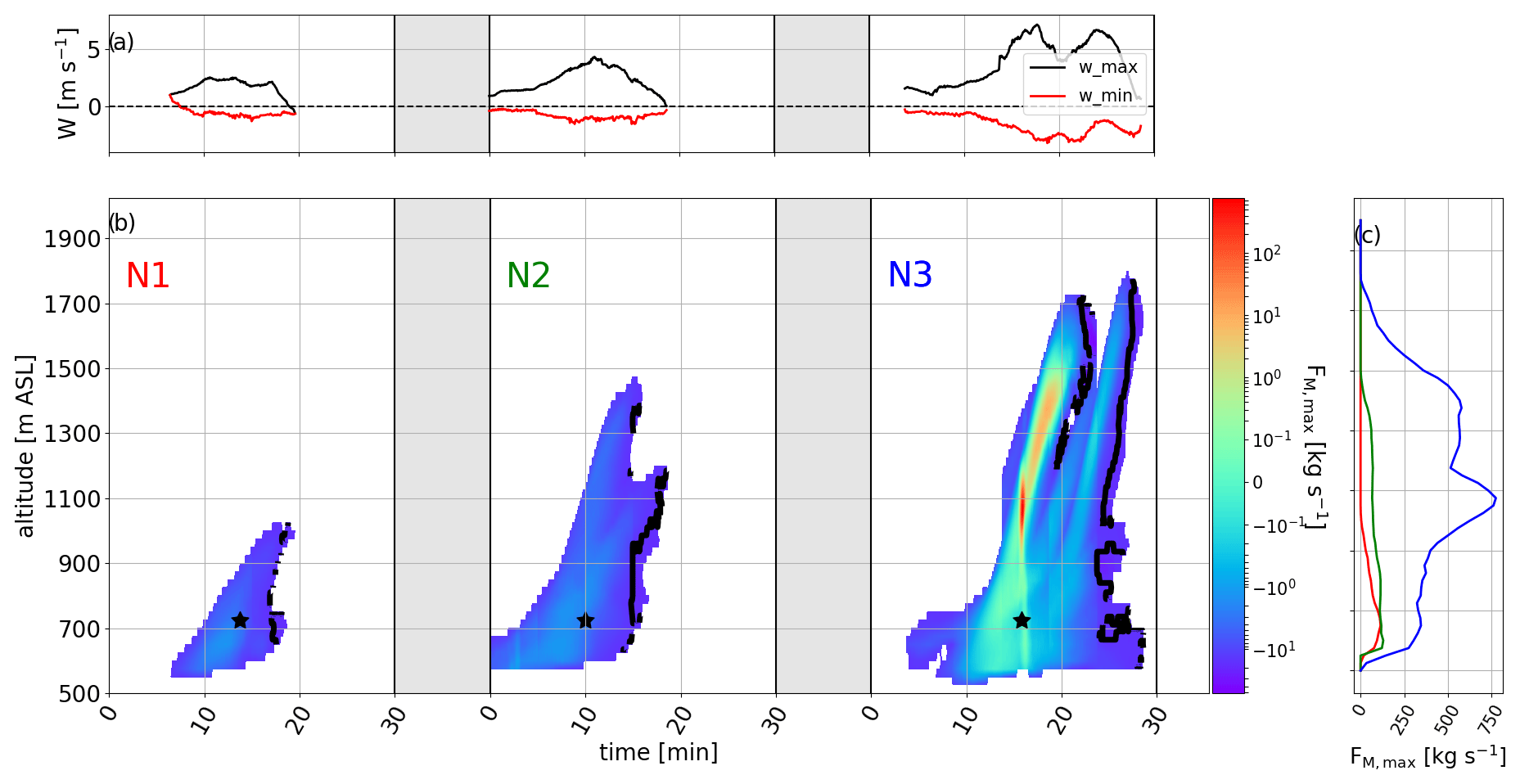
Figure 6 Life cycle of three clouds N1, N2, and N3 for (a) their minimum and maximum vertical wind, (b) their mass flux, and the (c) vertical profile of mass flux for each cloud. The black line in (b) corresponds to negative vertical flux. The black star represents altitude and time for static cloud exploration.

This individual study of clouds has permitted the description of heterogeneities in the horizontal and vertical structure of cumulus clouds, in particular with respect to LWC. An observational strategy with sufficiently high sampling resolution is necessary to capture these heterogeneities and is now conducted numerically by embedding the exploration of RPA in the HFS LES.

3.3 Exploration by RPA in LES

In this subsection, we simulate the capacity of RPA to explore the horizontal variabilities of the thermodynamic variables in a cloud. First, we demonstrate the concept using cloud N2 in a static state by neglecting its horizontal advection and time evolution. We then repeat for the same cloud N2 but taking into account its evolution with time (dynamic case). Also, the clouds N1 and N3 are explored in static mode.

3.3.1 Defining a pattern for a static cloud

For this subsection, the cloud is assumed to be static and the flight of the RPA is simulated by embedding the Meso-NH output in the Paparazzi autopilot module. The cloud shape and position as well as thermodynamical variables do not change during the exploration by the RPA. Horizontal wind is fixed to 0 m s⁻¹. To demonstrate the viability of the rosette pattern described in Sect. 2.2, a cross section at 150 m above cloud N2 base extracted at t=10 min is used (corresponding to the time when the cloud reaches its maximum volume) (Fig. 5). The location of the initial entrance in the cloud is random and is shown with a red arrow in Fig. 7a. In this case, the RPA conducts 11 transects at this altitude in the cloud.

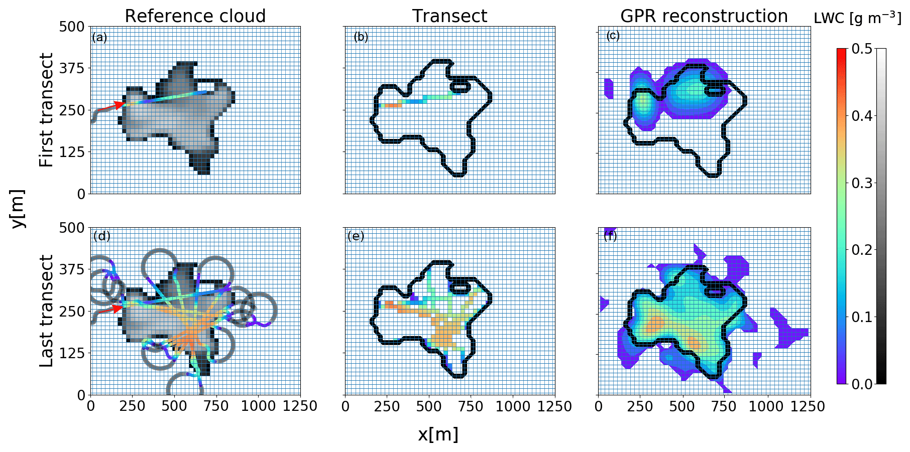
Figure 7 (a) Cross section of simulated cloud N2 at 150 m above cloud base in gray with the transect of the RPA; the color represents the LWC measured. (b) Reconstructed LWC in the cross section based on RPA transects. (c) Reconstructed LWC in the cross section with GPR mapping with λ_x=75 m. The first row corresponds to the end of the first transect, and the second row corresponds to all transects at the end of the exploration. The red arrow represents the first entrance in cloud N2 starting the rosette pattern (Sect. 2.2).

After each transect, the sampled horizontal distribution of LWC is reconstructed for the cross section (Fig. 7b). As the rosette pattern biases sampling of the geometric center, some regions in cloud N2 are oversampled, while regions toward the cloud edge are not measured at all. Nonetheless, to assess the ability of the rosette pattern to properly represent the horizontal cross section of the cloud, the probability density functions (PDFs) of reference LWC (Fig. 8a) and w (Fig. 8b) are compared with the PDFs of the reconstructed cloud cross section. The reference PDF of LWC (black line in Fig. 8a) has a main peak (15 % of cloudy grid cells) at 0.37 g m⁻³, corresponding to the cloud core, and 4 % of cloudy grid cells have an LWC that approaches the adiabatic value of 0.40 g m⁻³. The first transect results in an overestimation of high LWC values, while cloud edges (low LWC values) are underestimated, as also shown in Hoffmann et al. (2014). As the number of transects increases, the LWC biases decrease and the cumulative reconstructed PDF of the LWC approaches the reference distribution, but high values are still overestimated.

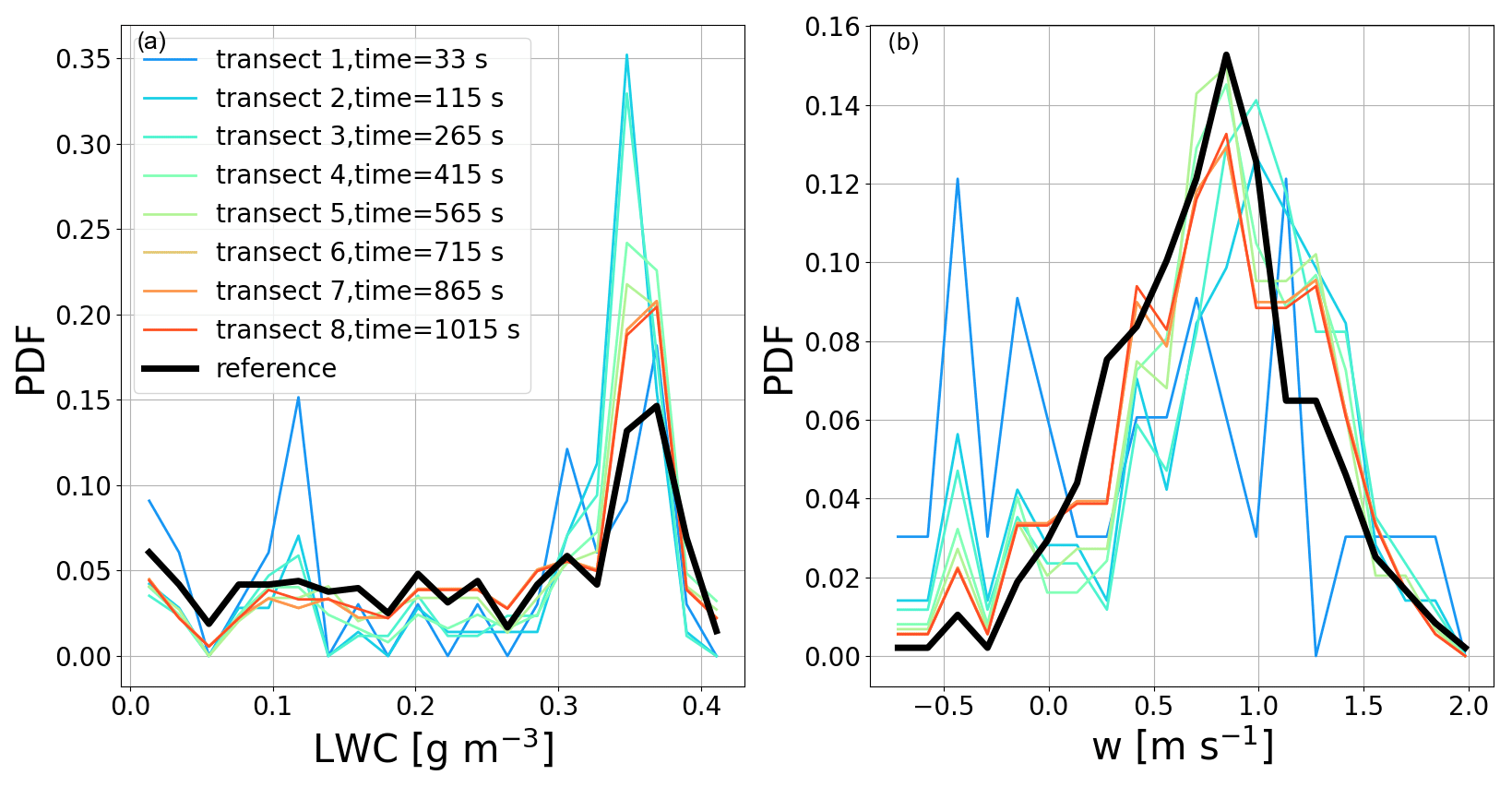
Figure 8 Reconstructed probability density function (PDF) of (a) LWC with time (color) compared to the reference of cloud N2 (black) at a height of 700 m a.s.l. (b) Same for vertical wind.

For vertical winds, the PDF (black line in Fig. 8b) represents a Gaussian distribution, and 15 % of model grids in the cloud cross section exhibit vertical wind between 0.7 and 0.9 m s⁻¹, corresponding to the peak of Gaussian distribution in the cloud. The cross-sectional area of downdrafts represents less than 10 % of total vertical wind. High values of updrafts are also overestimated with the first transects; however, the PDF converges to the reference PDF in less time than for LWC. In this study, the practice of only using the RPA observations to map the cloud is called the transect method. To compensate for the abovementioned biases of a single trajectory, simple forms such as a circle or ellipse provide a simple method to estimate the distribution of LWC and updrafts in the cross section. For example, an equivalent diameter (or the lengths of major and minor axes for an ellipse) can be estimated by an average transect length to retrieve a surface area for a circle or an ellipse. To derive a total LWC (LWC_tot) of the cross section, the volume of the reconstructed cloud section is multiplied by the average LWC, $\stackrel{\mathrm{‾}}{\text{LWC}}$. The transect method systematically underestimates the cloud volume section (area of the section multiplied by the 25 m thickness of the grid cell), while the cloud volumes reconstructed by circle and ellipse methods are more than twice the actual volume of the reference cross section, as shown in Fig. 9a. Clearly, none of these relatively simple methods are able to accurately reconstruct the cloud cross section (Fig. 9), particularly related to the fractal character of the borders of cloud cumulus. To address this deficiency in accurately reconstructing the cloud cross section using simple methods, we introduce a novel method that uses Gaussian process regression (GPR). Below, only the transect method (RPA observations) will be compared with GPR.

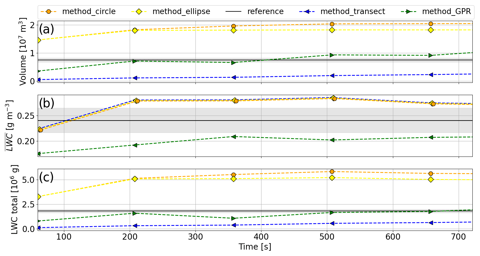
Figure 9 (a) Reconstructed cloud volume with circle method (orange line), ellipse method (yellow line), transect method (blue line), and GPR method (green line) compared to the reference volume (black line) for cloud N2 in static state at 700 m for one exploration. (b) The blue line corresponds to $\stackrel{\mathrm{‾}}{\text{LWC}}$ calculated by the transect method, the green line by the GPR method, and the dotted black line the reference $\stackrel{\mathrm{‾}}{\text{LWC}}$. (c) Same for integration of LWC in the section volume.

3.3.2 Gaussian process regression mapping

Gaussian process regression extends the spatial footprint of an observation by weighting its values with a Gaussian profile. It needs the definition of four length scales (${\mathit{\lambda }}_{t,z,y,x}$) representing spatial (z, y, x) and temporal (t) scales. For the static case, λ_t=∞ means that an earlier observation is considered to have the same weight as the last measurements (temporal variation is not taken into account).

To demonstrate the impact of length scales on GPR, sensitivity tests are carried out for cloud N2 using three different length scales corresponding to 2, 3, and 4 times the resolution of the simulation (50, 75, 100 m). The differences of the reconstructed map of LWC for the different length scales are shown in Fig. 10. For a horizontal length scale of 50 m, $\stackrel{\mathrm{‾}}{\text{LWC}}$ is underestimated in unsampled regions, consistent with a length scale that is too short (${\stackrel{\mathrm{‾}}{\text{LWC}}}_{\mathrm{reconstructed}}=\mathrm{0.20}$ g m⁻³ compared to ${\stackrel{\mathrm{‾}}{\text{LWC}}}_{\mathrm{reference}}=\mathrm{0.24}$ g m⁻³). To assess if the cross section of the cloud is correctly defined in its entirety, the root mean square error (RMSE) is also calculated and is equal to 8.92 g m⁻³. For a 75 m length scale, the reconstructed cross section represents the reference cloud with ${\stackrel{\mathrm{‾}}{\text{LWC}}}_{\mathrm{reconstructed}}=\mathrm{0.22}$ g m⁻³ and an RMSE of 5.71 g m⁻³. For the largest length scale, 100 m, the cross section of LWC extends beyond the edges of the reference cloud, also as expected for a length scale that is too large (${\stackrel{\mathrm{‾}}{\text{LWC}}}_{\mathrm{reconstructed}}=\mathrm{0.35}$ g m⁻³). The RMSE for a 100 m length scale increases significantly 14.89 g m⁻³. For the following analysis, the GPR mapping uses a 75 m length scale.

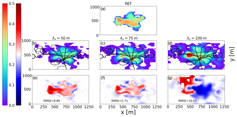
Figure 10 (a) The first row corresponds to a cross section of simulated cloud N2 at 150 m above the cloud base in color shade. The second row corresponds to a cross section of LWC reconstructed for cloud N2 with GPR for (b) λ_x=50 m, (c) λ_x=75 m, and (d) λ_x=100 m. The third row corresponds to the difference between the reference cross section and reconstructed cross section by GPR for the three length scales; RMSE is also shown.

3.3.3 Criteria for optimizing the exploration

In this section, different methods are applied to better characterize the heterogeneities of the thermodynamic variables and the total LWC. The exploration with a rosette pattern is repeated 10 times in the same cloud at the same altitude with different entrances. In each of these explorations, the reconstructed LWC_tot and $\stackrel{\mathrm{‾}}{\text{LWC}}$ are compared to the reference cloud every 60 s for 12 min. The reference LWC_tot and $\stackrel{\mathrm{‾}}{\text{LWC}}$ have values of 1.8×10³ g and 0.24 g m⁻³, respectively. Four sampling strategies are compared: a single RPA exploration just using observations along the trajectory (1-RPA) and with GPR mapping (1-RPA + GPR). A similar notation is used for the 2-RPA exploration.

The LWC_tot reconstructed for the four sampling strategies is shown in Fig. 11 with the standard deviation dispersion among the 10 flights shown as shading. For the first minute of exploration, the four methods underestimate the LWC_tot; however, after the second minute (about two to three transects), the 1-RPA and 2-RPA exploration with the GPR method calculates LWC_tot close to the reference LWC_tot, while with the two other methods without GPR, the LWC_tot stays significantly lower than the reference. After the third minute, the GPR method yields a stable $\stackrel{\mathrm{‾}}{\text{LWC}}$ within the reference $\stackrel{\mathrm{‾}}{\text{LWC}}\pm \mathrm{10}$ %, while 1-RPA and 2-RPA explorations without GPR never attain the reference LWC_tot. In addition, the standard deviation variability of LWC_tot is a factor of 3 less when using GPR.

Figure 11 Temporal evolution of reconstructed LWC total with the transect method with one RPA (blue line) or two RPA (red line) and with the GPR method with λ_x=75 m for a single RPA (green line) and two RPA (purple line). Colored shading areas represent LWC_tot± standard deviation for the 10 explorations for each 60 s. The black line corresponds to reference LWC_tot in the cloud N2 section in static state at 700 m, and the shaded gray area corresponds to ±10 % of LWC_tot.

It is possible to quantify the total LWC reliably around 180 s for exploration with two RPA + GPR mappings and 300 s for a single RPA + GPR mapping. Using Eq. (5) of Baker et al. (1984) allows relating the time needed for homogenization based on a turbulence kinetic energy dissipation rate of $\mathrm{0.89}\times {\mathrm{10}}^{-\mathrm{3}}$ m² s⁻³ at the level of 700 m (from the LES); these exploration times allow characterizing LWC heterogeneities caused by mixing having a characteristic length of 155 m with a single RPA and 72 m with two RPA. The simultaneous use of two RPA allows us to better characterize the thermodynamical changes in a cloud section in the case of a dynamic cloud.

Another stated objective of this study is to optimize the sampling strategy in order to best describe the thermodynamical heterogeneities in the cloud. To quantify this, the relative error is calculated as a sum of the difference between the reconstructed PDF and the reference PDF of LWC for each of the 20 bins of the distribution as

$$\begin{array}{}\text{(1)}& \text{relative error}={\displaystyle \frac{\mathrm{1}}{n_{\mathrm{bin}}}}\sum _i^{n_{\mathrm{bin}}}{\displaystyle \frac{\left|{\text{PDF}}_{\mathrm{ref},i}-{\text{PDF}}_{\mathrm{reconstructed},i}\right|}{{\text{PDF}}_{\mathrm{ref},i}}},\end{array}$$

where n_bin represents the number of bins, PDF_ref represents the reference PDF distribution of a variable noted i, and PDF_{reconstructed} represents the reconstructed PDF distribution with observations for the same variable i. Note that PDF_{reconstructed} is a cumulative PDF which takes into account previous transects.

The relative errors for the three methods are shown in Fig. 12. For the cloud N2, the time required for the single RPA without GPR to have a relative error below 0.5 is approximatively 350 s. With two RPA without GPR, the time required to have a relative error below 0.5 is reduced to 190 s. Figure 12 shows that the GPR provides a significant time saving, since an RPA associated with the GPR mapping takes only 120 s to have a relative error on the PDF below 0.5 and that two RPA operating simultaneously with a GPR mapping takes only 80 s.

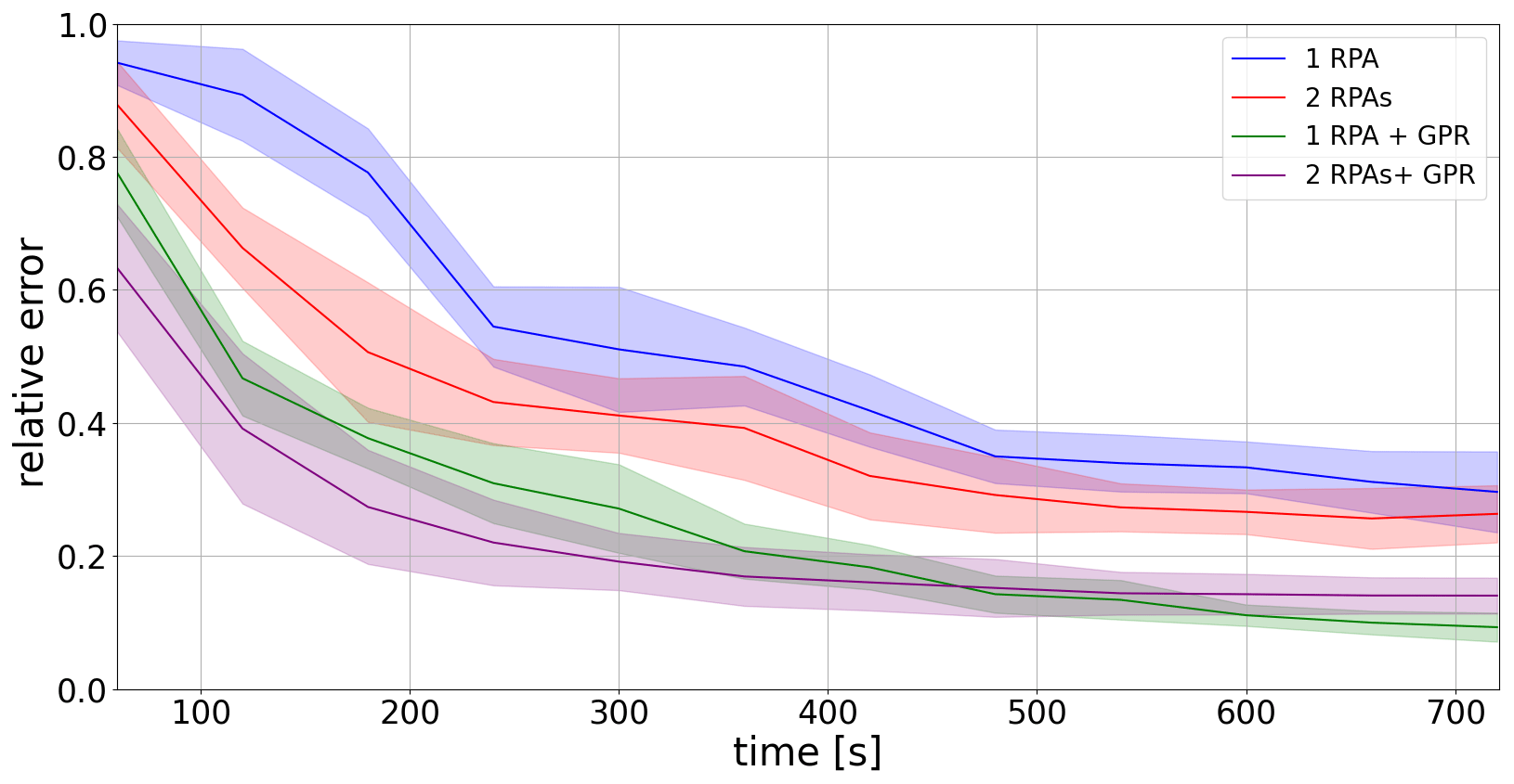
Figure 12 Temporal evolution of relative error in the PDF of the LWC distribution for a single RPA with the transect method (blue line) and GPR mapping (green line) as well as two RPA with the transect method (red line) and GPR mapping (purple line) during the exploration of cloud N2 in static state.

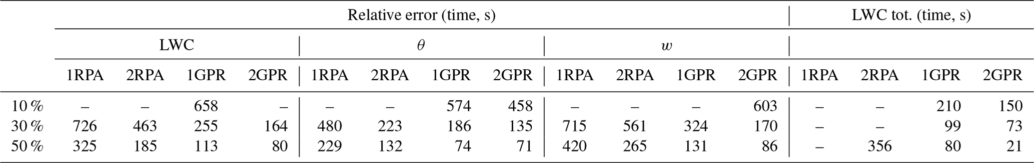
The time needed to reach different threshold relative errors of 10 %, 30 %, and 50 % for different variables (LWC, vertical wind, and potential temperature θ) is reported in Table 2, highlighting a significantly improved mapping of the cross section by using the GPR method.

Table 2 Time required to calculate relative error lower than 10 %, 30 %, and 50 % for the LWC, potential temperature, and vertical wind, W, of reference cloud and LWC_tot for the 1-RPA, 2-RPA, and 1-RPA + GPR exploration.

As described by Katzwinkel et al. (2014), the growth, maturity, and dissipation phases of a cloud life cycle have a timescale of minutes. Consequently, sampling of cloud cross section must also be completed within timescales of a few minutes. These results show that cloud cross sections are sufficiently well represented when using GPR methods.

3.3.4 Exploring clouds of different sizes

In this section, a generalization of the rosette pattern with the GPR method is applied to static clouds N1 and N3 at the time they reached their maximum cross-sectional area at 150 m above cloud base. Figure 13 shows the exploration with the rosette trajectories using GPR mapping.

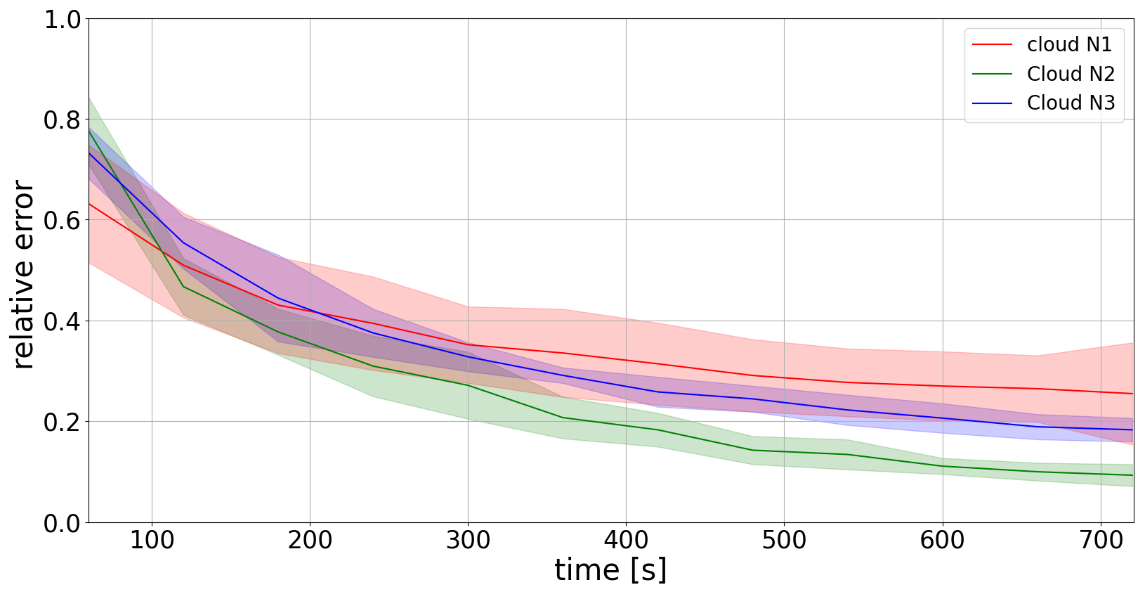
Figure 13 Temporal evolution of the relative error of LWC distribution for cloud N1 (red line), cloud N2 (green line), and cloud N3 (blue line) in static state. Shaded area corresponds to ± standard deviation for five explorations.

Length scales between 25 and 400 m were used to find an optimal length scale for clouds N1, N2, and N3. The sensitivity test was first applied to the cloud N2 (equivalent diameter 597 m), and the most efficient length scale was found to be 75 m. The same tests were performed for the other two clouds (cloud N1, equivalent diameter 240 m; cloud N3, equivalent diameter 1161 m), which resulted in similar length scales averaging 75±5 m for the three cases. The optimum length scale is independent of the cloud size (e.g., N1, N2, N3), suggesting that the length scale defined for GPR is related to the length scales of the strongest gradient of the parameter being explored (i.e., LWC in this case). The strongest gradient in LWC occurs in the cloud shell, which is generally two to three grid sizes (i.e., 50 to 75 m) of the LES. Length scales that are too small (i.e., 25 m) create “gaps” in the exploration, particularly for large clouds, while length scales that are too large blend the cloud shell and cloud core, which is relatively more important for small clouds.

When the dimension of the cloud is smaller than the turning radius (cloud N1), the exploration is pattern-limited in that the RPA cannot turn around and re-enter the cloud if the cloud itself is smaller than the RPA's turning radius. The relative error remains higher than 0.3 for the duration of the simulation. When the cloud radius is much larger than the turning radius there is simply more surface area to sample, which prolongs the exploration. For example, the relative error for cloud N3 only approaches 0.2 by the end of the exploration. Finally, Fig. 13 shows that when using GPR for a middle cloud (cloud N2), the relative error is below 0.2 midway through the exploration.

The results demonstrate that the rosette trajectory associated with a GPR mapping in a static environment is suitable for sampling thermodynamic and microphysical variables such as LWC or θ and w. We now assess the ability to measure thermodynamic and microphysical variables for a case in which the cloud evolves with time and in space (i.e., a dynamic case).

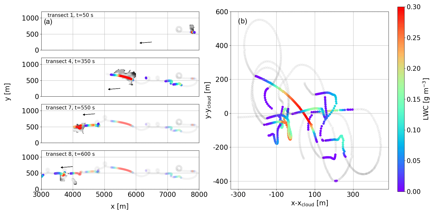
Figure 14 (a) Trajectories of exploration by following cloud N2 for four different transects. The colors represent the measured LWC, and the gray surface corresponds to the cross section of reference cloud N2 for the different times. The shading colors correspond to the past transects. The black arrow represents the direction of the advective wind. (b) Measured LWC in cloud frame during the exploration. The colored lines correspond to the values of measured LWC exceeding 10⁻² g m⁻³, and the gray lines correspond to the measured LWC below this threshold.

3.3.5 GPR reconstruction of a cloud evolving with time

In an evolving cloud, the RPA must constantly adjust its trajectory by taking into account the advection and spatial evolution of the cloud. In this subsection, an adaptive exploration follows the cloud in the cloud reference frame, which is redefined at each time step by accounting for the advective wind. To demonstrate the challenges in extending the analysis of a static environment (Sect. 3.3.1 to 3.3.4.) to a dynamic one, the adaptive exploration is applied here to cloud N2. For this case, the rosette pattern (Sect. 2.2) is also applied at 150 m above cloud base as for the static exploration. Cloud N2 vertical extent reaches 150 m above cloud base 4 min after its formation, and we start the exploration of cloud N2 at this time. The sampling strategy follows the rosette model in the cloud reference frame; the calculated center of the cloud moves relative to the advective wind. Observations of the cloud continue for 12 min (Fig. 14), corresponding to several transects in the cloud, until the moment of its dissipation (at the exploration level). The total horizontal distance covered is more than 5 km during this period. Figure 14 shows four periods of the dynamic exploration corresponding to the first, fourth, seventh, and eighth transects through the cloud N2. The first transect occurs during the growth phase of the cloud and does not traverse the region of maximum LWC, followed by the other transects in the maturity and dissipation phase of the cloud.

Figure 14b represents the RPA transects in a fixed frame where advection has been removed (in a Lagrangian reference frame). The cloud transects are 500–600 m long and map the evolution of the cloud's boundary.

Associated with these transects in the time-evolving cloud N2, the LWC measurements are shown in Fig. 15a. As expected, there is a clear underestimation of high LWC values when comparing LWC PDFs (Fig. 15b, transect 1). Between the fourth and seventh transects (300 to 550 s), the reference cloud is in a relatively stable mature phase. Once the center of the cloud is established, the exploration is efficient enough to reconstruct a PDF resembling that of the reference case with relative errors between 0.3 and 0.4. However, during the dissipation phase, the evolution of the cloud cross section is faster compared to the relatively stable mature phase and is not well represented by the PDF. These explorations are repeated several times, and the PDF descriptions are all more efficient in the mature phase (relative error around 0.3 to 0.4) than in the developing and dissipating phases. While GPR certainly improves the ability to reconstruct a cloud cross section, these results clearly show that to adequately observe the dissipation phase, the cross section must be reconstructed in less time. Averaging the multiple explorations (individual lines in Fig. 15b) yields similar results as a dynamic exploration with multiple uncoordinated RPA. These results show that the “noise” associated with the reconstructed probability function of LWC is greater during phases with more rapid evolution – therefore, to reduce the uncertainty, one needs to add RPA. In addition, Fig. 15b (50 and 600 s) shows that the RPA does not capture the higher LWC values associated with the core of the cloud when the cloud element is small, which is a result of a less efficient choice of exploration strategy.

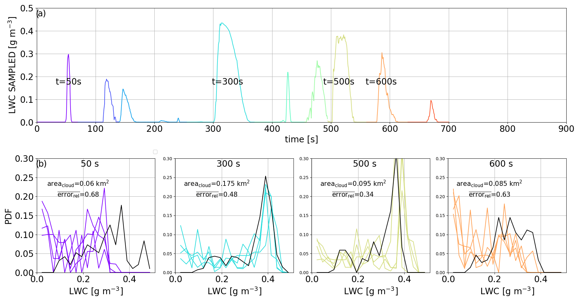
Figure 15 (a) Temporal evolution of LWC measured by RPA for different transects (colors). (b) Reconstructed probability function of LWC in color and by the reference in black for four transects of exploration (transects 1, 4, 7, 8).

4 Conclusions

The aim of this study is to determine an observational strategy for reconstructing thermodynamic properties of a cross section of a cumulus cloud without surface precipitation within a high-resolution large-eddy simulation (LES). We reproduce a high-resolution cumulus cloud field with the Meso-NH model in LES mode (with a 25 m spatial resolution), wherein the simulations are based on observations during the BOMEX field campaign. The high-resolution simulation serves as the basis for this study and compares well to an intercomparison LES study reported in Siebesma et al. (2003). By applying a novel cloud identification method to high-frequency 3D outputs, we isolated three clouds with different volumes (10⁻⁴ to 10⁻¹ km³) representative of the cumulus cloud population with varying lifetimes between 12 and 18 min. The goal of the sampling with a remotely piloted aircraft (RPA) is to reproduce a cloud cross section of liquid water content (LWC) and updraft velocity within a few minutes in order to follow the evolution of a cloud through its growth, maturity, and dissipation phases.

An autonomous RPA using a Paparazzi autopilot module is embedded into the LES to conduct an exploration of a cloud level using a rosette pattern. In a static environment (a cloud that does not evolve with time), the rosette pattern is applied to the cloud at the time and the level at which the surface area of its horizontal cross section is maximum. The rosette pattern is chosen for the adaptive trajectory since at each exit from the cloud, the RPA automatically conducts a half-turn to re-enter the cloud and conducts a subsequent transect through the geometric center of the cloud. The sampling of the cloud continues autonomously using a threshold LWC of 10⁻² g m⁻³ to determine if the RPA has entered or exited the cloud. The geometric center is calculated using a weighted sum of the LWC from the previous transects. The simulated observations serve to reconstruct different probability density function (PDF) distributions of LWC, vertical winds, volume, and total LWC.

Simple methods to derive a cross section using individual observations or assuming circular or elliptical forms of a cloud do not reproduce the LWC and its horizontal variability. Using only the observations from one or two RPA underestimates the amount and variability of LWC in the cloud cross-section. Assuming a circle or an ellipse yields a factor of 2 overestimation of total LWC in the cross section. We therefore explore another technique to expand the observational footprint using Gaussian process regression (GPR). GPR mapping extends individual measurements by applying a confidence level to the surrounding area and time related to a given length scale. The results show that GPR mapping significantly improves the reconstruction of the cloud cross section. A sensitivity test of the length scale used for GPR mapping indicates that the characteristic scale of 75 m is the best for reconstructing the horizontal LWC in a cloud. In fact, after three transects through the cloud, corresponding to a time of ≈200 s, the GPR mapping adequately reproduces total LWC (within a relative error of 10 %) and the PDF variability of the LWC (within 30 % relative error). The addition of a second RPA simultaneously with GPR mapping further improves the time of good restitution of the total LWC field and its distribution by reducing the time needed to obtain a correct LWC total value to 80 s.

To extend results of a static exploration to a realistic environment, the rosette pattern was applied to a cloud evolving in time and space in a dynamic environment. The GPR mapping method allows us to sample the thermodynamical distribution sufficiently well for a cloud during its maturity stage, which is the most stable phase of a cloud life cycle. However, during the growing and dissipating phases, a single RPA coupled with GPR is still insufficient to reproduce the temporal variability of the cloud life cycle.

In order to improve the observational capacity of airborne measurements, various methods are currently being explored, including the use of a camera system or radar to improve the cloud exploration, particularly for conditions when the cloud boundaries are broken or not well defined (e.g., a dissipating cloud).

To optimize the dynamic exploration of a cloud, at least two RPA are necessary. To improve our observations of the cloud life cycle, an improved coordination between the RPA is also necessary to avoid risk of collision and also to couple with different optimized adaptive trajectories.