the Creative Commons Attribution 4.0 License.
the Creative Commons Attribution 4.0 License.
 | 10 Jun 2022
Impact of 3D cloud structures on the atmospheric trace gas products from UV–Vis sounders – Part 3: Bias estimate using synthetic and observational data
Claudia Emde
Michel van Roozendael
Kerstin Stebel
Ben Veihelmann
Bernhard Mayer
Three-dimensional (3D) cloud structures may impact atmospheric trace gas products from ultraviolet–visible (UV–Vis) sounders. We used synthetic and observational data to identify and quantify possible cloud-related bias in NO2 tropospheric vertical column density (TVCD). The synthetic data were based on high-resolution large eddy simulations which were input to a 3D radiative transfer model. The simulated visible spectra for low-earth-orbiting and geostationary geometries were analysed with standard retrieval methods and cloud correction schemes that are employed in operational NO2 satellite products. For the observational data, the NO2 products from the TROPOspheric Monitoring Instrument (TROPOMI) were used, while the Visible Infrared Imaging Radiometer Suite (VIIRS) provided high-spatial-resolution cloud and radiance data. NO2 profile shape, cloud shadow fraction, cloud top height, cloud optical depth, and solar zenith and viewing angles were identified as the metrics being the most important in identifying 3D cloud impacts on NO2 TVCD retrievals. For a solar zenith angle less than about 40∘ the synthetic data show that the NO2 TVCD bias is typically below 10 %, while for larger solar zenith angles the NO2 TVCD is low-biased by tens of percent. The horizontal variability of NO2 and differences in TROPOMI and VIIRS overpass times make it challenging to identify a similar bias in the observational data. However, for optically thick clouds above 3000 m, a low bias appears to be present in the observational data.
- Article
(6977 KB) - Full-text XML
- Companion paper 1
- Companion paper 2
-
Supplement
(3781 KB) - BibTeX
- EndNote


Operational retrievals of tropospheric trace gases from space-borne spectrometers are based on the use of 1D radiative transfer models. To minimize cloud effects, generally only cloudless and partially cloudy pixels are analysed using simplified cloud contamination treatments based on radiometric cloud fraction estimates (e.g. Grzegorski et al., 2006; Stammes et al., 2008) and photon path length corrections based on oxygen collision pair (O2–O2) (Acarreta et al., 2004; Veefkind et al., 2016) or O2–A absorption band measurements (for example, the FRESCO and OCRA/ROCINN algorithms; see Koelemeijer et al., 2001; Wang et al., 2008; Loyola et al., 2018; Liu et al., 2021). In reality however, the impact of clouds can be much more complex, involving unresolved sub-pixel clouds, scattering of clouds in neighbouring pixels, and cloud shadow effects. In a model study, Merrelli et al. (2015) showed that 3D radiation scattering from unresolved boundary layer clouds may give significant biases in Orbiting Carbon Observatory-2 (OCO-2) retrievals of CO2 concentration. Massie et al. (2017, 2021) provided observational evidence of 3D cloud effects in OCO-2 CO2 retrievals and found them to be consistent with 3D radiative transfer simulations. For airborne and ground-based remote sensing, Schwaerzel et al. (2020, 2021) have shown the importance of accounting for 3D radiative transfer in air mass factor calculations when the atmosphere cannot be assumed to be horizontally homogeneous and when buildings are present.
In general, space-borne measurements of trace gases may be cloud-contaminated, and the presence of clouds may result in both positive and negative biases. It is thus vital to quantify the impact of clouds on trace gas retrievals and, if possible, envisage correction methods. Excluding cloud-contaminated pixels from analysis is not a viable option as this, for example, may give bias in long-term averages, as shown by Geddes et al. (2012) for NO2. Furthermore, the loss in data coverage when excluding partially cloudy scenes may become critical, especially for low-/medium-resolution sensors and for regions where the probability of cloud occurrence is high (e.g. Germany and other western European countries).
This paper is one of a series of three papers discussing the impact of 3D cloud structures on the atmospheric trace gas products from ultraviolet–visible (UV–Vis) sounders. The first paper by Emde et al. (2022) describes the synthetic data which is based on 3D radiative transfer model simulations utilizing realistic 3D clouds as input and is designed for validation of remote sensing trace gas retrievals. In the second paper, Yu et al. (2021) discuss trace gas retrieval and mitigation strategies in the presence of 3D cloud structures. In this paper, the bias due to 3D clouds is quantified using both synthetic and observational data.
We chose to study NO2, as it is an important measure of air quality and a key tropospheric trace gas measured by the atmospheric Sentinels (https://sentinel.esa.int, last access: 16 May 2022). The synthetic data, which ignore stratospheric NO2, were used to identify the cloud situations that give bias in tropospheric NO2 retrievals. The observational satellite data from the TROPOspheric Monitoring Instrument (TROPOMI) were used to investigate the presence of 3D cloud radiative transfer effects in real data. While the focus is on tropospheric NO2, the results are expected to be valid for other UV–Vis-derived trace gas products.
The paper first discusses the synthetic and observational data sets (Sect. 2). This is followed by a description of the various metrics used to identify cloud impacts (Sect. 3). In Sect. 4, the results are presented and discussed before the paper ends with some concluding remarks and an outlook in Sect. 5.
From the HD(CP)2 (https://hdcp2.eu/, last access: 16 May 2022) project, large eddy simulations (LESs) based on the ICOsahedral Non-hydrostatic atmosphere model (ICON; Dipankar et al., 2015; Zängl et al., 2015) are available for a region including Germany, the Netherlands, and parts of other surrounding countries. The model results were validated against ground- and satellite-based observational data by Heinze et al. (2017). This unique synthetic data set provides realistic input for 3D radiative transfer modelling. Hence, we adopted the study region to be the area covered by the LES. This region also covers part of the footprints of the upcoming Sentinel-4 and Sentinel-5 missions.
2.1 Synthetic satellite data
The synthetic satellite data comprise results from three sources: (1) high-resolution LES cloud data, (2) 3D radiative transfer modelling of satellite radiances with the LES cloud data as input, and (3) NO2 retrieval using the synthetic satellite radiances.
Within the HD(CP)2 project, the ICON model simulated realistic liquid and ice clouds with a horizontal spatial resolution of approximately 1.2×1.2 km2. Several weeks of simulations are available including all kinds of weather situations in Europe. We, however, utilize only one from 29 July 2014, 12:00 UTC, due to the computational burden of the radiative transfer simulations. The simulated scene includes all cloud types that are typical for Europe, such as shallow cumulus, cirrus, stratus, and also convective clouds. While focus is on Europe, the results/methods are expected to be general and thus applicable elsewhere.
The LES results were input to the 3D MYSTIC Monte Carlo radiative transfer model (Mayer, 2009; Emde et al., 2011) run within the libRadtran package (Mayer and Kylling, 2005; Emde et al., 2016) to generate synthetic observation spectra in the visible spectral range from 400 to 500 nm and in the O2–A band region from 755 to 775 nm (for further details see Emde et al., 2022; Yu et al., 2021). The spatial resolution of the simulated sensor was set to approximately 7×7 km2, corresponding to 98×104 pixels for the full LES domain. Note that each simulated sensor pixel includes 36 cloud pixels; hence the simulations include sub-pixel cloud inhomogeneity. The synthetic spectra were input to a NO2 retrieval algorithm which included two steps: first a differential optical absorption spectroscopy (DOAS) fit was performed using the QDOAS retrieval algorithm (Blond et al., 2007; De Smedt et al., 2008) to get the NO2 slant column densities; second the slant column densities were converted to vertical column densities using layer air mass factors (AMFs) based on the VLIDORT 1D radiative transport model (Spurr, 2006). The fitting window was between 425 and 495 nm, similar to the one used by Richter et al. (2011). The air mass factor was calculated at the middle of the fitting window, that is 460 nm. Cloud corrections were done using both O2–O2 and O2–A band (FRESCO, OCRA/ROCINN)-based methods (Yu et al., 2021). An example of retrieved NO2 tropospheric vertical column density (TVCD) for a synthetic case is shown in Fig. 1a. Note that the “true” NO2 is constant over the scene, with a column density of 1.6×10¹⁶ molec. cm−2, corresponding to a European tropospheric polluted NO2 profile from Levelt et al. (2009). Thus any differences between the retrieved and “true” NO2 TVCDs are due to the presence of clouds (Fig. 1b). The NO2 retrieval is further discussed by Yu et al. (2021).
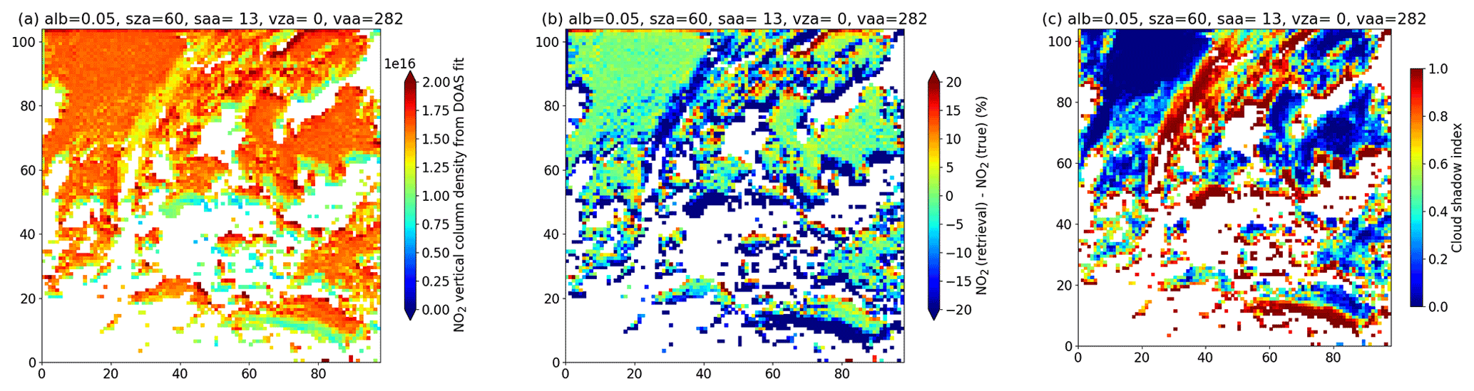
Figure 1(a) The retrieved NO2 TVCD for the low-earth-orbit geometry case, with albedo = 0.05, solar zenith angle = 60∘, solar azimuth angle = 13∘, satellite viewing angle = 0∘, and satellite azimuth angle = 282∘ (identical for all pixels). (b) The difference between the retrieved and the true NO2 TVCD. (c) The cloud shadow index; see Sect. 3.3 for details. The units on the axes are pixel numbers. White pixels are cloudy regions for which the retrieval was not performed.
While we discuss our synthetic results in connection with observational results from satellites in low-earth-orbit (LEO), simulations were also made for a geostationary orbit (GEO). Azimuth and zenith viewing and solar angles were chosen to resemble geometries for the study region when viewed by the TROPOspheric Monitoring Instrument (TROPOMI; Veefkind et al., 2012) and the future Ultra-violet Visible Near-infrared (UVN; https://sentinel.esa.int/web/sentinel/missions/sentinel-4, last access: 16 May 2022) instrument to be in geostationary orbit. In total 15 and 36 combinations of viewing and solar angles were simulated for the GEO case and LEO case, respectively (Emde et al., 2022). The surface was assumed to be snow-free and with constant albedo to simplify the interpretation of the results. In the visible (400–500 nm), simulations were done with albedos of 0, 0.05, and 0.2, while in the O2–A band region, an additional albedo of 0.5 was included to account for the potentially larger albedo in this part of the spectrum. Combining the sun-sensor geometries and visible albedo values, our simulated data set thus includes a total of 45 GEO cases and 108 LEO cases.
2.2 Observational satellite data
Both observational satellite spectrometer and imager data were utilized to investigate the presence of 3D cloud radiative transfer effects in real data. NO2 TVCD data were taken from the TROPOMI/S5P operational L2 NO2 tropospheric column product (van Geffen et al., 2021). TROPOMI/S5P was launched on 13 October 2017, and L2 NO2 data are available from 28 June 2018. It passes the Equator at 13:30 local time. S5P does not include an imager for cloud information. However, it flies in tandem with the Suomi National Polar-orbiting Partnership (S-NPP) satellite. The S-NPP payload includes the Visible Infrared Imaging Radiometer Suite (VIIRS) instrument, which may be used as an imager for TROPOMI. The difference in overpass time is slightly more than 4 min, and care must be taken with, for example, the movement of clouds when combining data from the two platforms (e.g. Trees et al., 2021). We used both VIIRS L1b and L2 data. The L1b reflectances were used for RGB plots and to produce various metrics; see Sect. 3. The L2 data include various cloud products of which we used the cloud mask, cloud shadow, cloud optical thickness, and cloud top height products. The TROPOMI data include the latitude and longitude of the corners of each TROPOMI pixel. This information was used to identify VIIRS pixels within each TROPOMI pixel.
Data within the study region roughly covering Germany and parts of neighbouring countries were collected for the periods 28 June 2018–15 October 2018 and 1 March 2019–30 June 2019 when the sun was sufficiently high on the horizon to avoid problems with NO2 retrievals for low sun (solar zenith angle (SZA) <60∘). The NO2 and cloud situations generally vary a lot for this region. In Fig. 2 an example of NO2 data from TROPOMI (Fig. 2b, c) and cloud optical depth (Fig. 2d), cloud top height (Fig. 2e) and cloud shadow fraction (Fig. 2f) from near-simultaneous VIIRS overpasses of Germany is shown. A distinct cloud shadow band is seen in Fig. 2a, d, and e, starting at about 50∘ N, 3∘ E and extending in the east/north-east direction.
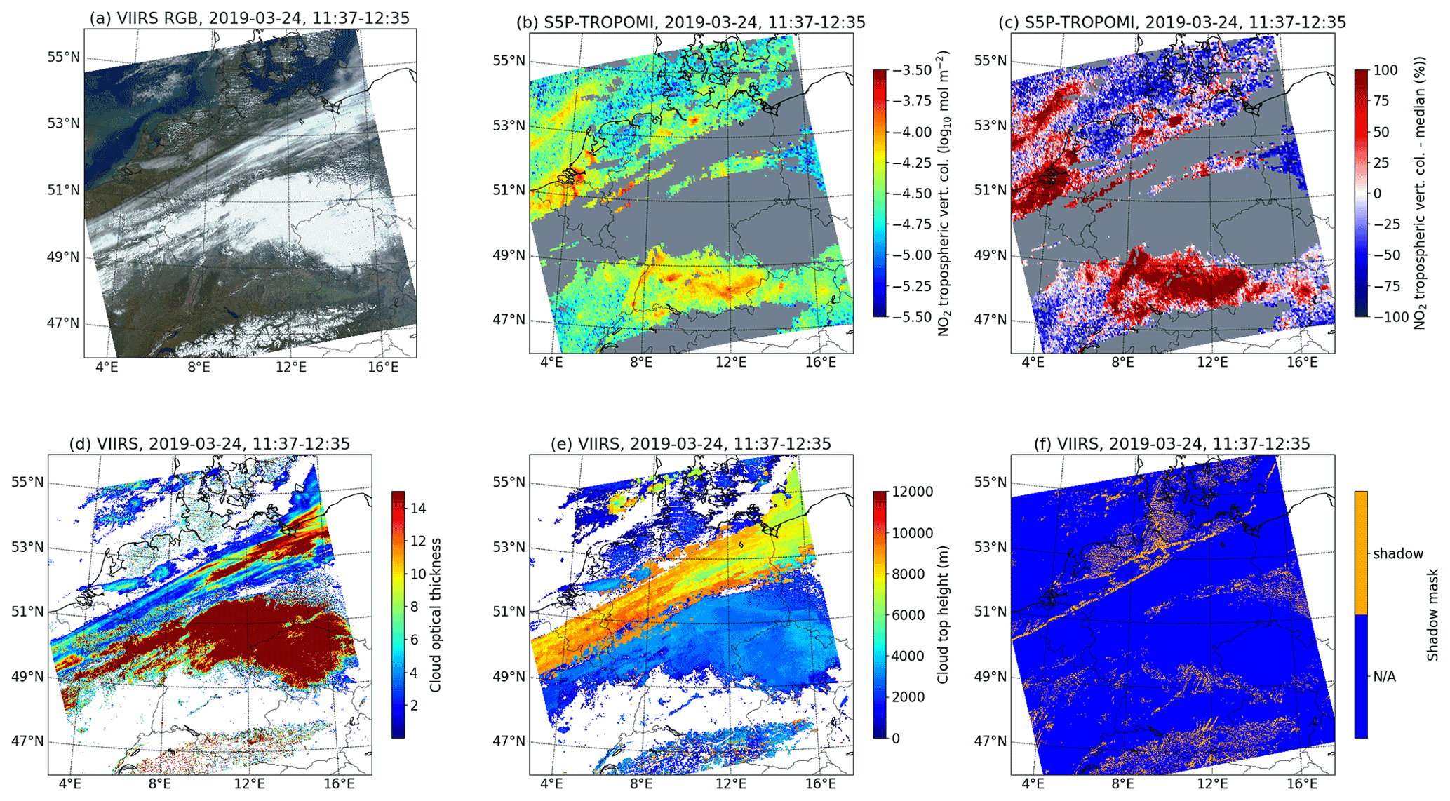
Figure 2(a) RGB composite of VIIRS bands M3, M4, and M5 (centred at 0.488, 0.555, and 0.672 µm). (b) The tropospheric NO2 vertical column density from TROPOMI. Only pixels with data quality value >0.95 are displayed. (c) The percentage difference of the NO2 column from the median over the study area. (d) The VIIRS cloud optical thickness. (e) The VIIRS cloud top height. (f) The VIIRS cloud shadow mask.
Several metrics were calculated to quantify cloud features and their possible connection with NO2 biases due to 3D cloud effects.
3.1 Cloud geometric and radiance fractions
Cloud fractions may be defined in several ways. We calculate the geometric cloud fraction, CFg, the radiometric cloud fraction, CFr, and the weighted radiometric cloud fraction, CFw.
The geometric cloud fraction for a TROPOMI pixel is defined as
where the sum is over all N VIIRS pixels within the TROPOMI pixel, and CMi is the VIIRS cloud mask, where CMi=1 for pixels identified as cloudy and CMi=0 otherwise.
The radiometric cloud fraction is the fraction of measured radiance reflected from clouds in a pixel (see also Grzegorski et al., 2006):
Here R is the observed reflectance, Rs the reflectance for a cloudless sky, and Rc the reflectance for an opaque cloud. For the O2–O2 cloud correction, CFr is calculated based on the reflectance at 460 nm, which is in the middle of the DOAS fitting window for NO2. For the FRESCO algorithm, CFr is determined by the reflectance in the 758–759 nm window band. Further details are described by Yu et al. (2021). We also define an average radiometric cloud fraction using the average of CFr calculated for each VIIRS M3 band pixel, centred at 0.488 µm, within a TROPOMI pixel:
where the sum is over all N VIIRS pixels within the TROPOMI pixel.
Finally, the weighted radiometric cloud fraction is defined as (Yu et al., 2021)
3.2 Cloud mask
No cloud mask was available for the LES-based synthetic data. In principle this may be calculated from the cloud optical thickness assuming some threshold. However, we chose to calculate a cloud mask similar to how it is done for several operational satellite products. We thus assume that pixels with reflectance larger than some threshold, R>Rt, are cloudy. The cloud mask was calculated from high-spatial-resolution radiance simulations at 0.55 µm of the synthetic cases described by Emde et al. (2022). A threshold of Rt=0.25, similar to Heinze et al. (2017), was adopted. It is noted that Barker et al. (2017) used Rt=0.15 for the GOES-13 0.65 µm band. Yang and Di Girolamo (2008) have shown that there may be overlap between clear and cloudy pixels, and hence some misclassification is unavoidable. Our slightly higher value of Rt potentially includes more cloud-contaminated pixels but also reflects that we are mainly working over land where surface albedo is higher than over ocean.
3.3 Cloud shadow fraction and cloud shadow index
The VIIRS cloud shadow mask algorithm is geometry-based and described by Hutchison et al. (2009). They compared the MODIS MOD35 product which uses spectral signatures to identify cloud shadows with geometry-based approaches and state that the latter “are far superior to those predicted with the spectral procedures”. A cloud shadow detection algorithm using only TROPOMI data has been described by Trees et al. (2021). It was, however, not available for this study.
The cloud shadow fraction, CSF, for a TROPOMI pixel is defined as
where the sum is over all N VIIRS pixels within the TROPOMI pixel, and CSMi is the VIIRS cloud shadow mask, where CSMi=1 for pixels identified as cloud shadow and CSMi=0 otherwise.
For the LES we define the cloud shadow index (CSI) as a surrogate for a cloud shadow product as follows:
Here E0=1 is the direct transmittance at the surface for an atmosphere with no molecular absorption nor clouds or aerosol. The direct transmittance, Eθ,ϕ, at the surface for a solar zenith angle of θ and solar azimuth angle ϕ was calculated with the MYSTIC model. It also does not include molecular absorption nor aerosol; however, it includes clouds, which are fully accounted for in 3D geometry and with the 3D cloud fields in higher spatial resolution than the TROPOMI pixel size. The CSI is zero for pixels with no cloud shadow and 1 if a pixel is fully in the cloud shadow. The CSI clearly and unambiguously identifies cloud shadow regions as it is based solely on sun, cloud, and surface geometry. An example of the CSI is given in Fig. 1c.
3.4 H metric
For a TROPOMI pixel the H metric is the standard deviation of VIIRS band reflectances divided by the mean of the VIIRS reflectances within the TROPOMI pixel. It is an estimate of the variation of radiance within the TROPOMI pixel and has been used earlier by, for example, Massie et al. (2017) as a metric for the impact of 3D clouds on CO2 retrievals. In the presence of sub-pixel clouds, the H metric is expected to increase as the horizontal cloud inhomogeneity increases. In the absence of clouds, the H metric is expected to be small. However, for cloud-free pixels with large variations in surface albedo, the H metric may still be large, and conversely, for a completely cloudy pixel the H metric may be small. Thus, it may not be used without care to unambiguously identify cloud inhomogeneity. From the VIIRS data we calculate the H metric for the M3, M4, and M5 bands centred at 0.488, 0.555, and 0.672 µm respectively.
3.5 Absorbing aerosol index
Clouds have an effect on the UV absorbing aerosol index (AAI). It is thus of interest to investigate possible relationships between the AAI and the cloud shadow fraction and the NO2 TVCD. The AAI is a measure of the UV colour of a cloud-, aerosol-, and shadow-free 1-D atmosphere–surface model with respect to the measured UV colour (de Graaf et al., 2005). When absorbing aerosols are present, the AAI tends to be positive, while the AAI is approximately zero or negative in the presence of clouds (see, for example, Kooreman et al., 2020; Penning de Vries et al., 2009). We use the TROPOMI AAI product to investigate relationships between the AAI and the NO2 TVCD.
For both the synthetic and observational data, the aim is to compare the NO2 TVCD for cloud-affected cases with the true NO2 TVCD and identify potential biases. This is straightforward for the synthetic data as the true NO2 TVCD is known. For the observational data, the true NO2 TVCD unaffected by clouds is in general not known and is difficult to estimate due to the horizontal variability of NO2. An attempt to estimate the true NO2 TVCD from the observational data is discussed in Sect. 4.2, which also includes the analysis of the observational data.
4.1 Synthetic satellite data
For the synthetic data, the fully cloudy pixels were not simulated due to the computational burden; see Emde et al. (2022) for details. To further filter for the presence of clouds, the NO2 TVCDs were retrieved for pixels where the radiometric cloud fraction CFr<0.3 for all LEO and GEO cases. The retrieval tries to correct for the presence of remaining clouds by including a standard photon path length correction based on absorption by the oxygen collision pair O2–O2 or the O2–A band as described by Yu et al. (2021). An example of the retrieved NO2 TVCD and the bias is shown in Fig. 1a and b, while the cloud shadow index is shown in Fig. 1c.
For three LEO cases, the difference between the retrieved and “true” NO2 TVCDs versus the cloud shadow index is shown in Fig. 3. The cloud shadow impact is seen to increase as the solar zenith angle increases. The number of pixels with NO2 TVCD differences % is 0.2 % for a solar zenith angle of 20∘ (Fig. 3a), 4.1 % for 40∘ (Fig. 3b), and 20.1 % for 60∘ (Fig. 3c). As the solar zenith angle increases, a linear relationship appears between the NO2 TVCD difference and the CSI, as indicated by the black lines and corresponding R2 values. The increase of the cloud shadow impact with increasing solar zenith angle is due to the increase in cloud shadow size for larger solar zenith angles for geometrical reasons; see Emde et al. (2022) for a detailed discussion.
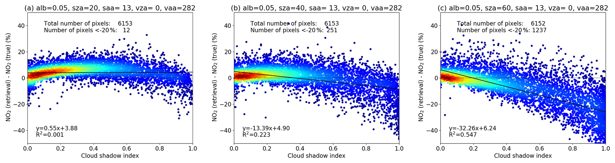
Figure 3The difference between the retrieved and “true” NO2 TVCDs versus the cloud shadow index for three low-earth-orbiting geometry cases. Results are shown for cloud-filtered pixels and solar zenith angles of (a) 20, (b) 40, and (c) 60∘, albedo = 0.05, solar azimuth angle = 13∘, satellite azimuth angle = 0∘, and satellite viewing angle = 282∘. The black lines are linear fits, and the fit parameters and R2 are given in the individual plots. The data in (c) are for the case presented in Fig. 1.
For the cloud correction of the AMF, the weighted radiometric cloud fraction, CFw, is used as described by Yu et al. (2021). The effect of increasing CFw is shown in Fig. 4, where the NO2 AMF bias (1D AMF–3D AMF) is plotted as a function of CFw for all GEO and LEO geometries. The retrieval bias is binned in CFw bins with 2 % steps, which gives more than 5000 pixels in each bin when the CFw<75 %. The bias may have several causes. The NO2 profile and surface albedo input give differences between the VLIDORT, used in the retrieval, and the MYSTIC radiative transfer model (RTM), used for the 3D simulations, on the order of 1 % (Emde et al., 2022; Yu et al., 2021). As discussed by Yu et al. (2021), the NO2 retrieval error due to the use of a simple cloud correction scheme is generally less than 20 % for nearly cloud-free cases (CFw<50 %). Therefore, pixels with a NO2 retrieval bias >20 % are likely to be affected by cloud shadow effects. For both geometries, the NO2 AMF bias is high (median of 20 %) and with a large range (0 %–65 %) for CFw<1 %. For these clear pixels, there is a significant number of pixels with the retrieval bias >20 %, and this is attributed to cloud shadow effects. The bias decreases to 0 % when the CFw is between 1 %–3 %. The bias range increases slightly with increasing CFw: about 75 % of the pixels have a positive bias for large CFw for GEO geometry, while there are comparatively more pixels with a negative bias for LEO geometry. The solar zenith angle is the same for the LEO and GEO cases. However, the solar azimuth angle and the sensor viewing zenith and azimuth angles are different. For the LEO and GEO geometries studied, see Emde et al. (2022) for details; the sun is to the south of the study region. This implies that a relatively large portion of cloud shadows are on the northern sides of the clouds. These cloud shadows are partly hidden from GEO satellites but may be visible from the LEO satellite instrument with a nadir view of Earth, thus giving different sensitivity to cloud shadows for LEO and GEO geometries. More than 15 % of the pixels have a bias larger than 20 % for CFw>50 % for both GEO and LEO geometries.
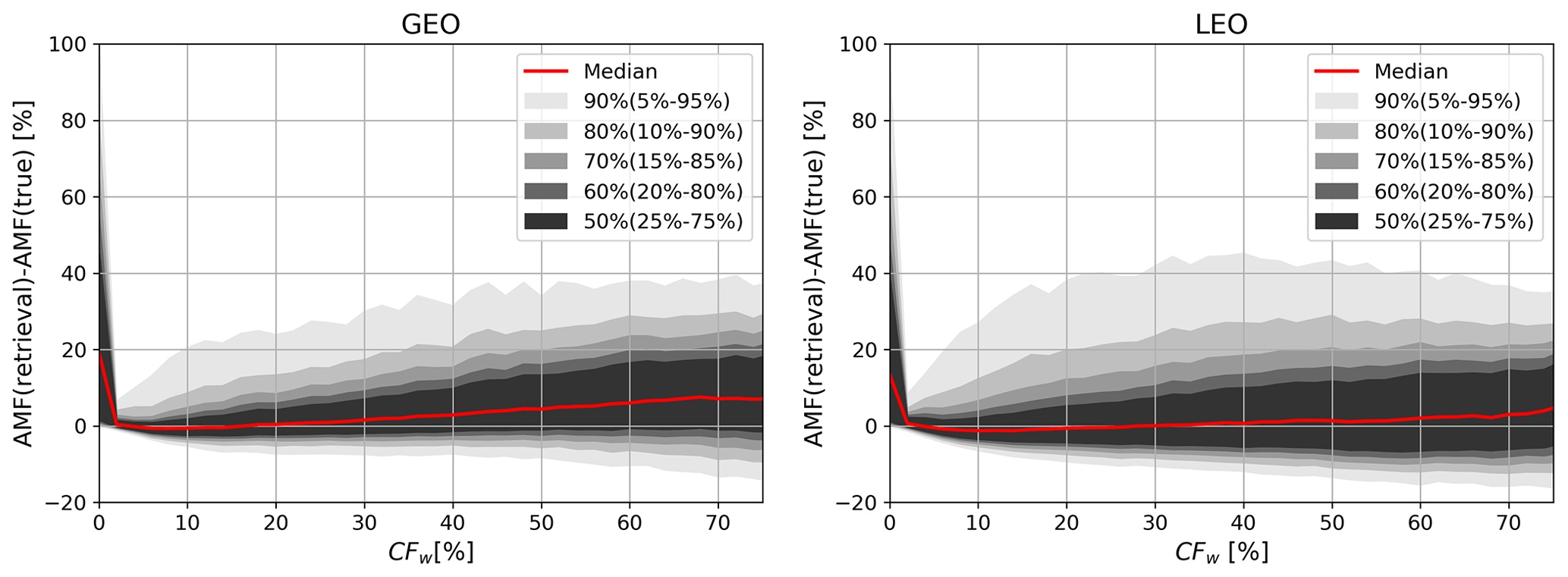
Figure 4Distribution of the NO2 AMF bias as a function of the weighted radiometric cloud fraction, CFw, for geostationary and low-earth-orbiting geometries. Results are shown for the retrieval using the O2–O2 cloud correction. Results are similar for the O2–A band-based cloud correction.
Figure 5 shows the number of pixels that satisfy these conditions for all the LEO and GEO geometries. For the geostationary geometry, the number of pixels with retrieval bias >20 % is up to about 1000 or 10.6 % (out of 9400 pixels for a single case). This number increases with surface albedo and SZA; the difference between surface albedos of 0.05 and 0.2 is about 150 to 400 pixels. As discussed above, the increase with solar zenith angle is due to larger cloud shadow for geometrical reasons. With respect to the albedo dependence, Emde et al. (2022) showed that the relative 3D–1D difference in reflectance increases with increasing surface albedo. Furthermore, Yu et al. (2021) showed that this gives increased differences in O2–O2 and FRESCO cloud-corrected AMFs with increasing surface albedo. This number also strongly depends on the solar azimuth angle (SAA), and the difference between SAAs of 315 and 45∘ is more than 25 %. For low-earth-orbiting geometry, the number of pixels with bias >20 % increases with surface albedo and SZA as well, and it is up to 1600 (17 %) for high surface albedo of 0.2 and SZA of 60∘.
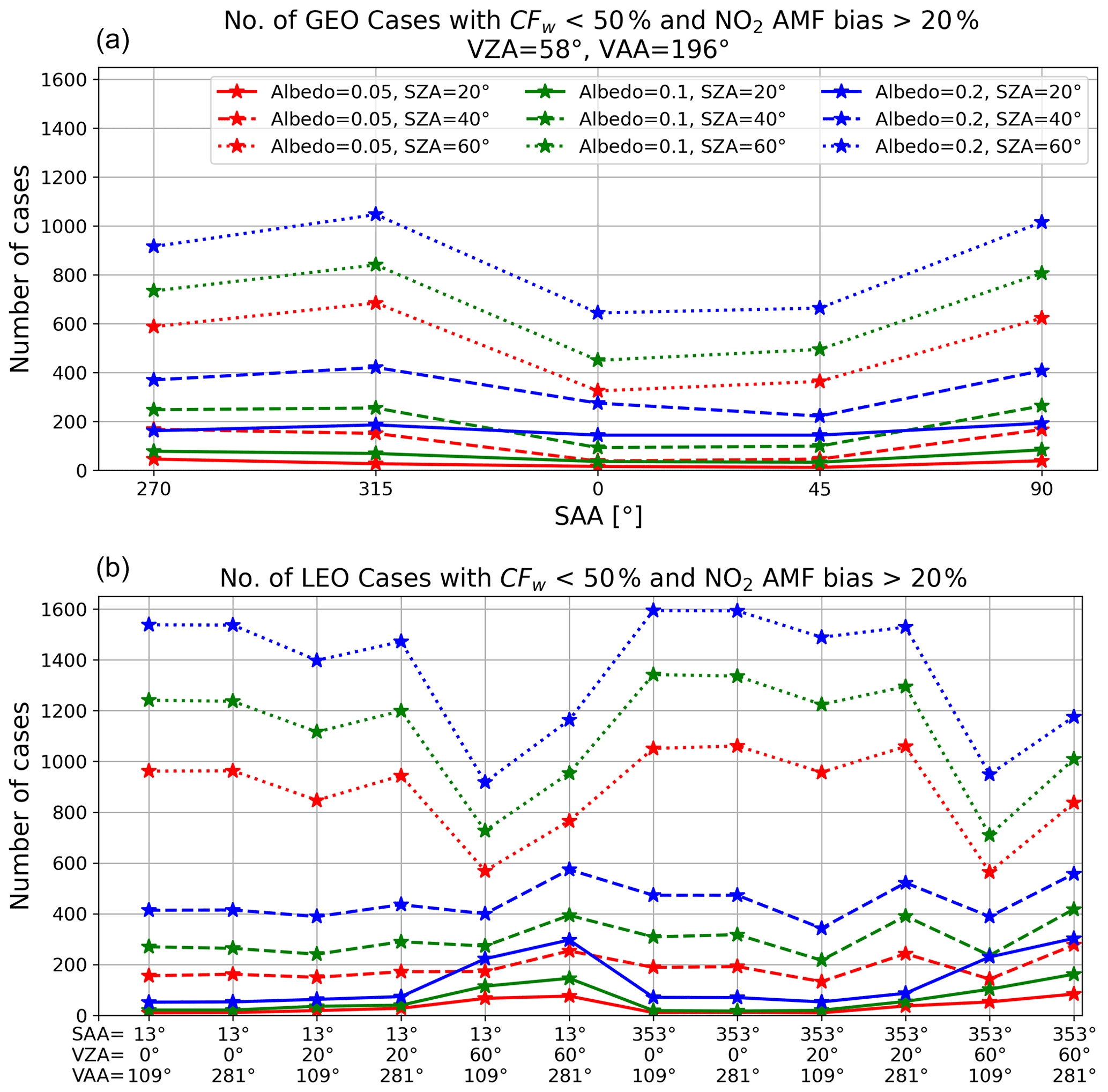
Figure 5Number of pixels with weighted radiometric cloud fraction CFw<50 % and NO2 AMF bias >20 % for geostationary (a) and low-earth-orbiting (b) geometries. The data points are connected by lines for increased readability. Different line styles indicate different SZAs, while line colours are used for the surface albedo as given in the annotation. For the geostationary geometry, the solar azimuth angle (SAA) for each case is given on the x-axis label, while for the low-earth-orbiting geometry, the viewing zenith angle (VZA) and viewing azimuth angle (VAA) are given in addition. The total number of pixels for a single case is 9400.
To identify the localization of the pixels with NO2 AMF bias >20 %, maps of the number of cases with NO2 AMF bias >20 % were made as shown in Fig. 6. Generally, the majority of pixels with large NO2 AMF bias are found in cloud-free regions close to cloud edges. For a solar zenith angle around 40∘, most pixels will have an AMF bias below 20 % if the distance to the cloud edge is more than about 10 km. For a solar zenith angle of 60∘, this distance increases to about 20 km. The distance depends on a number of factors such as cloud top height, cloud optical depth, and surface albedo. This is further discussed and quantified for box clouds in the accompanying paper by Yu et al. (2021). Figure 7 shows maps of the maximum retrieval bias for each pixel. As above, cloudy data (CFw>50 %) are excluded from the analysis. The maximum bias is usually less than 60 % over the northwest region (x= 30–50, y= 70–100) where there is an ice cloud with small optical thickness (<10). In the centre of the map, the bias is often higher than 100 %; the pixels around are covered by a convective cloud with large vertical extent and optical thickness >100. Figure 8 shows under which geometry the maximum bias is observed. Pixels with maximum biases <20 % are not shown. In general, the maximum bias is obtained at high SZA (60∘), and for GEO cases, the bias also depends on the solar azimuth angle. Maximum biases are found on the east/west side of the cloud when the sun is in the . Note that this dependency on GEO geometry is particular for the region, and thus solar and viewing conditions, studied. This dependency is not seen for the LEO geometry as for LEO geometry, the local daily revisit time is the same and thus also the solar azimuth. A further summary of the LEO and GEO cases is provided in Fig. S1.
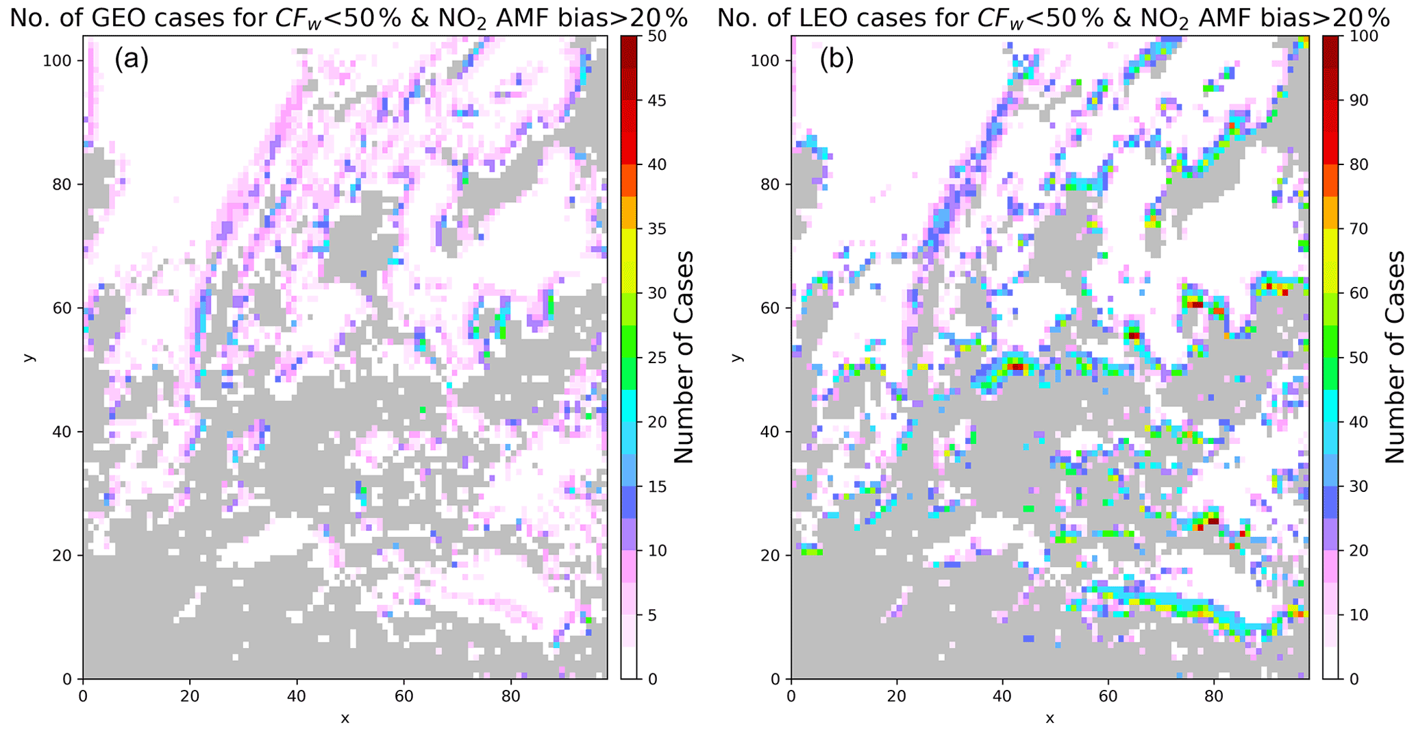
Figure 6The number of cases with CFw<50 % and NO2 AMF bias >20 % for each pixel for GEO (a) and LEO geometries (b). The x and y axes represent pixel number in the longitude and latitude direction. Grey shaded pixels indicate cloudy pixels.
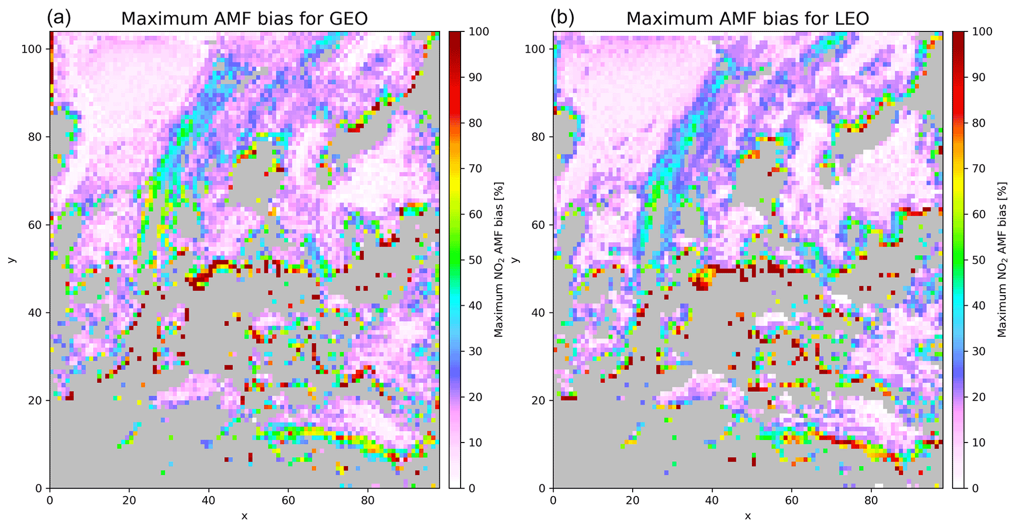
Figure 7Maximum NO2 AMF bias for each pixel for (a) geostationary geometry and (b) low-earth-orbiting geometry.
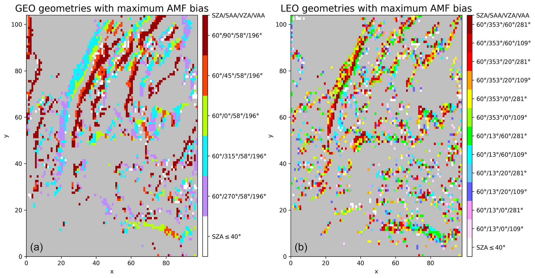
Figure 8Geometry for the largest AMF bias for each location for (a) geostationary geometry and (b) low-earth-orbiting geometry. Only the pixels with maximum bias >20 % are shown.
These results show that the solar zenith angle is of prime importance for 3D cloud impacts and that the impact increases with increasing solar zenith angle. This is for geometry reasons, which cause the cloud shadow to increase as the solar zenith angle increases. Also, as the viewing zenith angle increases, a larger, potentially cloud-shadow-impacted, horizontal surface area will be viewed for geometry reasons, and thus the cloud shadow effect increases with increased viewing zenith angle. Both under- and overestimates of the NO2 TVCD occur in pixels close to clouds. The underestimates are due to cloud shadows; thus the cloud shadow fraction is a cloud feature metric that may be used to identify affected pixels (Fig. 3). However, while for large solar zenith angles, pixels affected by cloud shadows are mostly underestimated, overestimates occur for all solar zenith angles and are mostly present for low cloud shadow fractions (Fig. 3) and increase for large surface albedo (dashed blue lines in Fig. S1). Thus, cloud features in neighbouring pixels, such as cloud top altitude and cloud optical thickness, are also of importance (Emde et al., 2022).
According to box cloud simulations presented by Emde et al. (2022) and Yu et al. (2021), the cloud enhancement effect is of similar magnitude as the cloud shadow effect. For the synthetic data, the enhancement effect is present but is smaller in magnitude than the cloud shadow effect; see blue lines in Fig. S1. This is most likely due to cloud-enhancement-affected pixels being identified as cloudy and thus not analysed. Also the synthetic data indicate that the smaller the solar zenith angle is, the larger the chances are for cloud enhancements between 5 % and 10 % for low-earth-orbit satellites (data not shown). The differences are largest for large satellite viewing angles (60∘) and may thus indicate enhancement due to the satellite partly viewing sun-illuminated cloud sides. For geostationary geometry, this effect is not present. This is due to differences in the solar azimuth angles for the two geometries. However, in magnitude, this effect has a much smaller impact than cloud shadows.
For large SZA (60∘) and low albedo, the number of pixels with NO2 TVCD underestimated by more than % is 12.0 % and 18.3 % for GEO and LEO geometries, respectively. For comparison, Lorente et al. (2017) estimated the structural uncertainty (differences in retrieval methodology) in the tropospheric NO2 AMF to be 42 % over polluted regions and 31 % over unpolluted regions. These differences are mostly driven by the uncertainty in the a priori NO2 profile, cloud properties, and surface albedo. Thus, while smaller than the structural uncertainty, 3D cloud impacts constitute an additional significant error source for polluted conditions and large SZA. Note that the different cloud correction schemes (O2–O2 and O2–A band) are normally within 10 % (not shown), and this number may be interpreted as the level of uncertainty introduced by these correction schemes.
4.2 Observational satellite data
As shown in Sect. 2.1 for the synthetic data, the NO2 bias may be on the order of tens of percent and are largest for large solar zenith angles. We thus searched TROPOMI and VIIRS data for cases with cloud shadows and large solar zenith angles.
While the true NO2 TVCD is known for the synthetic data, for the observational data, the true NO2 TVCD unaffected by clouds is not known. In order to have a reference or true NO2 TVCD to compare with, we look at neighbour pixels in a 3×3 pixel matrix, where the pixel of interest is in the centre. The true NO2 TVCD is then taken to be the average of cloud-free neighbours with NO2 retrieval quality value >0.95. Obviously this choice of true NO2 TVCD has its problems, including that neighbours may also be affected by clouds and that NO2 TVCDs may have large spatial gradients; see, for example, Fig. 2b, which shows the NO2 TVCD, and Fig. 2c, which shows the percentage difference of the NO2 TVCD to the area median NO2 TVCD.
For specific cloud band cases and associated cloud band shadows, the NO2 TVCD appears low-biased when the cloud is optically thick and the cloud shadow fraction >0.0 compared to when the cloud shadow fraction is zero; see Figs. S3 and S4.
For general cases, we looked for NO2 TVCD biases due to clouds for the months of October 2018 and March 2019 when the solar zenith angle is between 50 and 60∘ for the study region (covering approximately Germany, the Netherlands, and parts of other surrounding countries; see Sect. 2). A total of 1 023 081 TROPOMI pixels and 45 926 808 VIIRS pixels were collected for the study region and October 2018 and March 2019. To quantify possible cloud shadow effects and factors that impact it, TROPOMI pixels with NO2 retrieval data quality value >0.95 and cloud shadows were selected for further analysis. A NO2 retrieval with the data quality value >0.95 was reported for 367 584 (36 %) of the pixels. The VIIRS cloud mask identified 70.7 % of the VIIRS pixels to be cloudy, indicating that clouds were the main reason for reducing the NO2 retrieval quality for the majority of the TROPOMI pixels. Of the 367 584 pixels with high NO2 retrieval data quality, a total of 129 180 (35 %) were affected by cloud shadows according to the VIIRS cloud shadow product. Of the 45 926 808 VIIRS pixels, 13 438 968 (29.3 %) were cloud-free. Of these cloud-free VIIRS pixels, 17.8 % contained cloud shadows. This number is lower than the number of TROPOMI pixels affected by cloud shadows as is to be expected due to the higher spatial resolution of VIIRS. Note that this number pertains to months of the year for which we expect cloud shadow effects to be large due to the large solar zenith angles. For months of the year with smaller solar zenith angles, this number may well be smaller. The pixels affected by cloud shadows were further analysed to understand which parameters have the largest impact on the NO2 TVCD. In order to have a reference NO2 TVCD to compare the centre pixel value with, only centre pixels which have one or more cloud-free neighbours with NO2 retrieval quality value >0.95 were included. This restriction reduced the number of TROPOMI pixels to be analysed from 129 180 to 39 011. For these pixels, the difference between the centre pixel NO2 TVCD and the average of the NO2 TVCD in the cloud-free neighbours (ΔNO2) is shown as a function of cloud height maximum of neighbour pixels in Fig. 9. For this data subset, clouds are mostly found at high (about 10 000 m) and low (about 1900 m) altitudes, with relatively more clouds at the higher altitudes. This is qualitatively in agreement with Noel et al. (2018). They reported cloud fractions as estimated from a lidar on board the International Space Station. For Europe (their Fig. 5b), they report a similar cloud vertical behaviour, albeit for a different time of year (July, June, and August). The subset of TROPOMI pixels presented in Fig. 9 shows both high and low NO2 TVCD biases with a median NO2 TVCD bias of −1.4 % and maximum of the Gaussian kernel density probability density function estimate of −0.7 %. Thus, for this subset of TROPOMI pixels, no significant cloud shadow effect is visible in the NO2 TVCD. As stated above, no true observational NO2 TVCD is available as for the synthetic data. Furthermore, clouds and thus cloud shadows may have moved between VIIRS and TROPOMI overpasses. This may be a reason for the lack of a clear cloud shadow effect in this data subset.
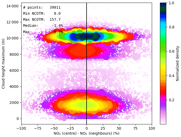
Figure 9The difference between the centre pixel NO2 TVCD and the average of the NO2 TVCD in the cloud-free neighbours as a function of cloud height maximum of neighbour pixels. The median of the difference is given in the legend together with the maximum of a Gaussian kernel-density probability density function estimate of the data points. The size of the data points illustrates the maximum cloud optical thickness in neighbour pixels (NCOTM). It varies between the minimum and maximum NCOTM values given in the legend.
This subset of data was further binned according to the maximum cloud height of neighbour pixels and the maximum slant cloud optical thickness , where COT is the VIIRS cloud optical thickness) of neighbour pixels as given in Table 1. Furthermore, only TROPOMI pixels where the maximum slant cloud optical thickness and maximum cloud top height are in the same neighbour pixel were included. This reduced the data set to 18 029 pixels.
Table 1Binning of parameters used to quantify the cloud shadow effect.

The NO2 TVCD bias density as a function of the cloud shadow fraction for the SCOT bins and maximum cloud heights is shown in Fig. 10. As the cloud height increases (from bottom row to top row in Fig. 10), the cloud shadow fraction increases because generally the cloud shadow within a pixel geometrically increases with cloud height when the cloud is larger than the pixel size. For the low clouds, the median NO2 TVCD bias varies between −1.2 % and 0.2 % for SCOT <15. For SCOT >15 the median NO2 TVCD bias is −2.9 %. For the medium-height clouds, the median NO2 TVCD bias for SCOT >15 increases in magnitude to −5.8 %. For smaller SCOT, the median NO2 TVCD bias is negative and varies between −0.8 % and −3.4 %. For the high clouds, the median NO2 TVCD bias is between −0.3 % and 1.6 % for SCOT <7. For larger SCOT, the median NO2 TVCD bias is −0.9 %, −8.7 %, and −15.1 % (7< SCOT <10, 10< SCOT <15, 15< SCOT <300).
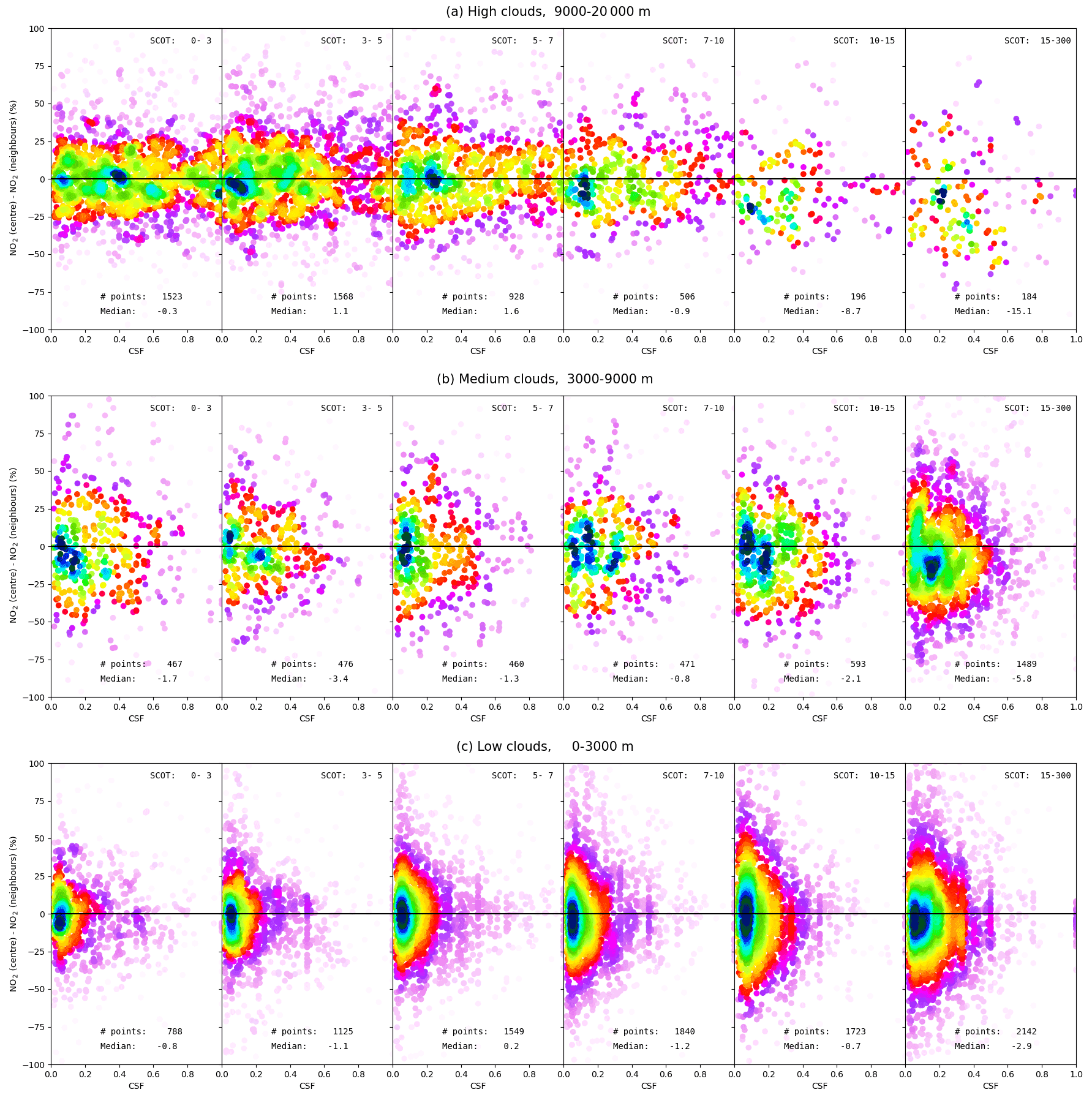
Figure 10The NO2 bias density as a function of the cloud shadow fraction. The data are binned into slant cloud optical thickness bins for high (a), medium (b) and low (c) clouds. See text for further details.
For all cloud heights, the median NO2 TVCD bias is negligible for SCOT <7. For low and medium clouds, there is a negative bias for the largest SCOT. For the high clouds the bias is pronounced for SCOT >10. Thus, the median NO2 TVCD bias increases with cloud height and with slant cloud optical thickness. It is noted that for individual pixels the bias may be larger and both positive and negative. We use a neighbour pixel as the true NO2 value. This assumes that only the cloud shadow effect is the reason for the NO2 TVCD bias. In reality there are horizontal gradients in the NO2 TVCD for numerous other causes as well, including local emissions and transport. Also, the difference in overpass time between VIIRS and TROPOMI may give differences in the clouds and cloud shadows viewed by the two instruments.
Finally it is noted that for the 129 180 pixels which were affected by cloud shadows, the number of pixels with cloud-free neighbours where % is 45.7 %. Under the assumption that this number is applicable to all TROPOMI pixels affected by cloud shadows, about 16 % of TROPOMI pixels for which NO2 TVCD retrievals were done with a high-quality value may be impacted by cloud effects larger than 20 % for solar zenith angles between 50 and 60∘. Of these, about half of the NO2 TVCDs are overestimated and half underestimated. The underestimate is clearly linked to cloud shadow effects. The overestimate may be due to in-scattering or horizontal gradients in NO2 concentrations and thus a wrong cloud-shadow-free NO2 TVCD true value. These two processes may, however, not be distinguished in the observed data set.
In this study we have investigated the impact of 3D clouds on NO2 TVCD retrievals from UV–Vis sounders. Both synthetic and observational data have been used to identify and quantify possible biases in NO2 TVCD retrievals. The synthetic data were based on high-resolution LES results which were input to the MYSTIC 3D radiative transfer model. The simulated visible spectra for low-earth-orbiting and geostationary geometries were analysed with standard NO2 retrieval methods, including operational cloud corrections. Profiles of NO2 for polluted conditions, with increased NO2 in the lower atmosphere below cloud tops, were considered as cloud shadow effects are not important for background NO2 conditions where the amount of NO2 below the cloud top is relatively small compared to the tropospheric column. For the observational data, the NO2 products from TROPOMI were used, while VIIRS provided high-spatial-resolution cloud data. Both single cases and overall statistics were calculated. The main findings are as follows:
-
The following metrics were identified as being the most important in identifying 3D cloud impacts on NO2 retrievals: NO2 profile shape, cloud shadow fraction, cloud top height, cloud optical thickness, and solar zenith and viewing angles.
-
Analysis of the synthetic data shows that for low-earth and geostationary orbit geometries, 89 % and 93 %, respectively, of the retrieved NO2 TVCDs are within 10 % of the actual column for small solar zenith angles. For large solar zenith angles, the numbers decrease to 53 % and 61 %.
-
The synthetic data show that in general the NO2 TVCD bias is slightly larger for low-earth-orbiting geometries than for geostationary geometries. This is due to differences in viewing geometry, where, for the mid-latitude targets studied here, the sun-target-detector geometry overall sees fewer cloud shadows for geostationary geometry.
-
For a solar zenith angle less than about 40∘, the synthetic data show that the NO2 TVCD bias is typically below 10 %, while for larger solar zenith angles the NO2 TVCD is low-biased by tens of percent. The horizontal variability of NO2 and differences in TROPOMI and VIIRS overpass times makes it challenging to identify a similar bias in the observational data. However, for optically thick clouds above 3000 m, a low bias appears to be present in the observational data.
-
For clearly identified cloud shadow bands from optically thick clouds in the observational data, the NO2 TVCD appears low-biased when the cloud shadow fraction >0.0 compared to when the cloud shadow fraction is zero. If it is assumed that the clouds are the main reason for the variations in the NO2 TVCD over the cloud shadow band, i.e. the NO2 field is assumed to be horizontally homogeneous, then these cloud shadow band cases are examples of how cloud shadows give underestimates of NO2 TVCD, in agreement with the theoretical findings.
The above conclusions suggest that further work is required on 3D cloud radiative impacts. For this future work the following topics may be considered:
-
As shown in this study, 3D radiative simulation of high-resolution satellite instrument spectra with realistic 3D cloud input is fully achievable. However, to cover all possible atmospheric situations on Earth, more high-spatial-resolution LES results may be needed. Furthermore, 3D RT modelling is demanding on computer resources and requires careful interpretation and analysis of the output. It is expected that such modelling efforts may prove useful, not only for trace gas retrieval algorithm studies, but also for cloud detection and cloud microphysics retrievals and more.
-
For future missions, including the Meteosat Third Generation (MTG) Flexible Combined Imager (FCI) and the Meteorological Operational Satellite Second Generation METimage (formerly known as VII-Visible and Infrared Imager), a cloud shadow product is needed for assessing and mitigating 3D cloud impacts. Experience with the VIIRS cloud shadow product (large changes between versions1) suggests that independent verification with ground measurements may be of use. Such validation is non-trivial and possibly requires new experimental approaches for measurements of both cloud shape and trace gas spatial variation at sub-pixel resolution.
The libRadtran software used for the radiative transfer simulations is available from http://www.libradtran.org (last access: 16 May 2022; Mayer et al., 2022). The QDOAS software for DOAS retrieval of trace gases is available from https://uv-vis.aeronomie.be/software/QDOAS/ (last access: 16 May 2022; Danckaert et al., 2022).
VIIRS data were accessed through the NOAA Comprehensive Large Array-Data Stewardship System (CLASS; https://www.avl.class.noaa.gov, last access: 16 May 2022; NOAA, 2022). TROPOMI data were downloaded from https://s5phub.copernicus.eu/ (last access: 16 May 2022; Copernicus Open Access Hub, 2022).
The supplement related to this article is available online at: https://doi.org/10.5194/amt-15-3481-2022-supplement.
AK collected and analysed the satellite data. CE constructed the synthetic data set. HY performed the NO2 retrieval. AK, CE, and HY analysed the synthetic data and defined the paper structure and content. MvR, KS, BV, and BM contributed to conceptualization and methodology.
At least one of the (co-)authors is a member of the editorial board of Atmospheric Measurement Techniques. The peer-review process was guided by an independent editor, and the authors also have no other competing interests to declare.
Publisher’s note: Copernicus Publications remains neutral with regard to jurisdictional claims in published maps and institutional affiliations.
We thank Nikolaos Evangeliou for helping with ERA5 data. We would also like to thank the two anonymous referees for their comments.
This research has been supported by the European Space Agency (contract no. 4000124890/18/NL/FF/gp).
This paper was edited by Folkert Boersma and reviewed by two anonymous referees.
Acarreta, J. R., De Haan, J. F., and Stammes, P.: Cloud pressure retrieval using the O2–O2 absorption band at 477 nm, J. Geophys. Res., 109, D05204, https://doi.org/10.1029/2003JD003915, 2004. a
Barker, H. W., Qu, Z., Bélair, S., Leroyer, S., Milbrandt, J. A., and Vaillancourt, P. A.: Scaling properties of observed and simulated satellite visible radiances, J. Geophys. Res. Atmos., 122, 9413–9429, https://doi.org/10.1002/2017JD027146, 2017. a
Blond, N., Boersma, K. F., Eskes, H. J., van der A, R. J., Van Roozendael, M., De Smedt, I., Bergametti, G., and Vautard, R.: Intercomparison of SCIAMACHY nitrogen dioxide observations, in situ measurements and air quality modeling results over Western Europe, J. Geophys. Res., 112, D10311, https://doi.org/10.1029/2006JD007277, 2007. a
de Graaf, M., Stammes, P., Torres, O., and Koelemeijer, R. B. A.: Absorbing Aerosol Index: Sensitivity analysis, application to GOME and comparison with TOMS, J. Geophys. Res., 110, D01201, https://doi.org/10.1029/2004JD005178, 2005. a
Copernicus Open Access Hub: S5P, https://s5phub.copernicus.eu/, last access: 16 May 2022. a
Danckaert, T., Fayt, C., Van Roozendael, M., De Smedt, I., Letocart, V., Merlaud, A., and Pinardi, G.: QDOAS [code], https://uv-vis.aeronomie.be/software/QDOAS/, last access: 16 May 2022. a
De Smedt, I., Müller, J.-F., Stavrakou, T., van der A, R., Eskes, H., and Van Roozendael, M.: Twelve years of global observations of formaldehyde in the troposphere using GOME and SCIAMACHY sensors, Atmos. Chem. Phys., 8, 4947–4963, https://doi.org/10.5194/acp-8-4947-2008, 2008. a
Dipankar, A., Stevens, B., Heinze, R., Moseley, C., Zängl, G., Giorgetta, M. A., and Brdar, S.: Large eddy simulation using the general circulation model ICON, J. Adv. Model. Earth Sy., 7, 963–986, https://doi.org/10.1002/2015MS000431, 2015. a
Emde, C., Buras, R., and Mayer, B.: ALIS: An efficient method to compute high spectral resolution polarized solar radiances using the Monte Carlo approach, J. Quant. Spectrosc. Ra., 112, 1622–1631, 2011. a
Emde, C., Buras-Schnell, R., Kylling, A., Mayer, B., Gasteiger, J., Hamann, U., Kylling, J., Richter, B., Pause, C., Dowling, T., and Bugliaro, L.: The libRadtran software package for radiative transfer calculations (version 2.0.1), Geosci. Model Dev., 9, 1647–1672, https://doi.org/10.5194/gmd-9-1647-2016, 2016. a
Emde, C., Yu, H., Kylling, A., van Roozendael, M., Stebel, K., Veihelmann, B., and Mayer, B.: Impact of 3D cloud structures on the atmospheric trace gas products from UV–Vis sounders – Part 1: Synthetic dataset for validation of trace gas retrieval algorithms, Atmos. Meas. Tech., 15, 1587–1608, https://doi.org/10.5194/amt-15-1587-2022, 2022. a, b, c, d, e, f, g, h, i, j, k
Geddes, J. A., Murphy, J. G., O'Brien, J. M., and Celarier, E. A.: Biases in long-term NO2 averages inferred from satellite observations due to cloud selection criteria, Remote Sens. Environ., 124, 210–216, https://doi.org/10.1016/j.rse.2012.05.008, 2012. a
Grzegorski, M., Wenig, M., Platt, U., Stammes, P., Fournier, N., and Wagner, T.: The Heidelberg iterative cloud retrieval utilities (HICRU) and its application to GOME data, Atmos. Chem. Phys., 6, 4461–4476, https://doi.org/10.5194/acp-6-4461-2006, 2006. a, b
Heinze, R., Dipankar, A., Henken, C. C., Moseley, C., Sourdeval, O., Trömel, S., Xie, X., Adamidis, P., Ament, F., Baars, H., Barthlott, C., Behrendt, A., Blahak, U., Bley, S., Brdar, S., Brueck, M., Crewell, S., Deneke, H., Girolamo, P. D., Evaristo, R., Fischer, J., Frank, C., Friederichs, P., Göcke, T., Gorges, K., Hande, L., Hanke, M., Hansen, A., Hege, H.-C., Hoose, C., Jahns, T., Kalthoff, N., Klocke, D., Kneifel, S., Knippertz, P., Kuhn, A., van Laar, T., Macke, A., Maurer, V., Mayer, B., Meyer, C. I., Muppa, S. K., Neggers, R. A. J., Orlandi, E., Pantillon, F., Pospichal, B., Röber, N., Scheck, L., Seifert, A., Seifert, P., Senf, F., Siligam, P., Simmer, C., Steinke, S., Stevens, B., Wapler, K., Weniger, M., Wulfmeyer, V., Zängl, G., Zhang, D., and Quaas, J.: Large-eddy simulations over Germany using ICON: a comprehensive evaluation, Q. J. Roy. Meteor. Soc., 143, 69–100, https://doi.org/10.1002/qj.2947, 2017. a, b
Hutchison, K. D., Mahoney, R. L., Vermote, E. F., Kopp, T. J., Jackson, J. M., Sei, A., and Iisager, B. D.: A Geometry-Based Approach to Identifying Cloud Shadows in the VIIRS Cloud Mask Algorithm for NPOESS, J. Atmos. Ocean. Tech., 26, 1388–1397, https://doi.org/10.1175/2009JTECHA1198.1, 2009. a
Koelemeijer, R. B. A., Stammes, P., Hovenier, J. W., and de Haan, J. F.: A fast method for retrieval of cloud parameters using oxygen A band measurements from the Global Ozone Monitoring Experiment, J. Geophys. Res., 106, 3475–3490, 2001. a
Kooreman, M. L., Stammes, P., Trees, V., Sneep, M., Tilstra, L. G., de Graaf, M., Stein Zweers, D. C., Wang, P., Tuinder, O. N. E., and Veefkind, J. P.: Effects of clouds on the UV Absorbing Aerosol Index from TROPOMI, Atmos. Meas. Tech., 13, 6407–6426, https://doi.org/10.5194/amt-13-6407-2020, 2020. a
Levelt, P., Veefkind, J., Kerridge, B., Siddans, R., de Leeuw, G., Remedios, J., and Coheur, P.: Observation Techniques and Mission Concepts for Atmospheric Chemistry (CAMELOT), European Space Agency, Noordwijk, the Netherlands, Report RP-CAM-KNMI-050, 2009. a
Liu, S., Valks, P., Pinardi, G., Xu, J., Chan, K. L., Argyrouli, A., Lutz, R., Beirle, S., Khorsandi, E., Baier, F., Huijnen, V., Bais, A., Donner, S., Dörner, S., Gratsea, M., Hendrick, F., Karagkiozidis, D., Lange, K., Piters, A. J. M., Remmers, J., Richter, A., Van Roozendael, M., Wagner, T., Wenig, M., and Loyola, D. G.: An improved TROPOMI tropospheric NO2 research product over Europe, Atmos. Meas. Tech., 14, 7297–7327, https://doi.org/10.5194/amt-14-7297-2021, 2021. a
Lorente, A., Folkert Boersma, K., Yu, H., Dörner, S., Hilboll, A., Richter, A., Liu, M., Lamsal, L. N., Barkley, M., De Smedt, I., Van Roozendael, M., Wang, Y., Wagner, T., Beirle, S., Lin, J.-T., Krotkov, N., Stammes, P., Wang, P., Eskes, H. J., and Krol, M.: Structural uncertainty in air mass factor calculation for NO2 and HCHO satellite retrievals, Atmos. Meas. Tech., 10, 759–782, https://doi.org/10.5194/amt-10-759-2017, 2017. a
Loyola, D. G., Gimeno García, S., Lutz, R., Argyrouli, A., Romahn, F., Spurr, R. J. D., Pedergnana, M., Doicu, A., Molina García, V., and Schüssler, O.: The operational cloud retrieval algorithms from TROPOMI on board Sentinel-5 Precursor, Atmos. Meas. Tech., 11, 409–427, https://doi.org/10.5194/amt-11-409-2018, 2018. a
Massie, S. T., Schmidt, K. S., Eldering, A., and Crisp, D.: Observational evidence of 3-D cloud effects in OCO-2 CO2 retrievals, J. Geophys. Res.-Atmos., 122, 7064–7085, https://doi.org/10.1002/2016JD026111, 2017. a, b
Massie, S. T., Cronk, H., Merrelli, A., O'Dell, C., Schmidt, K. S., Chen, H., and Baker, D.: Analysis of 3D cloud effects in OCO-2 XCO2 retrievals, Atmos. Meas. Tech., 14, 1475–1499, https://doi.org/10.5194/amt-14-1475-2021, 2021. a
Mayer, B.: Radiative transfer in the cloudy atmosphere, Eur. Phys. J. Conferences, 1, 75–99, 2009. a
Mayer, B. and Kylling, A.: Technical note: The libRadtran software package for radiative transfer calculations - description and examples of use, Atmos. Chem. Phys., 5, 1855–1877, https://doi.org/10.5194/acp-5-1855-2005, 2005. a
Mayer, B., Emde, C., Gasteiger, J., and Kylling, A.: libRadtran [code], http://www.libradtran.org, last access: 16 May 2022. a
Merrelli, A., Bennartz, R., O'Dell, C. W., and Taylor, T. E.: Estimating bias in the OCO-2 retrieval algorithm caused by 3-D radiation scattering from unresolved boundary layer clouds, Atmos. Meas. Tech., 8, 1641–1656, https://doi.org/10.5194/amt-8-1641-2015, 2015. a
NOAA (National Oceanic and Atmospheric Administration): Comprehensive Large Array-data Stewardship System (CLASS), NOAA [data set], https://www.avl.class.noaa.gov, last access: 16 May 2022. a
Noel, V., Chepfer, H., Chiriaco, M., and Yorks, J.: The diurnal cycle of cloud profiles over land and ocean between 51∘ S and 51∘ N, seen by the CATS spaceborne lidar from the International Space Station, Atmos. Chem. Phys., 18, 9457–9473, https://doi.org/10.5194/acp-18-9457-2018, 2018. a
Penning de Vries, M. J. M., Beirle, S., and Wagner, T.: UV Aerosol Indices from SCIAMACHY: introducing the SCattering Index (SCI), Atmos. Chem. Phys., 9, 9555–9567, https://doi.org/10.5194/acp-9-9555-2009, 2009. a
Richter, A., Begoin, M., Hilboll, A., and Burrows, J. P.: An improved NO2 retrieval for the GOME-2 satellite instrument, Atmos. Meas. Tech., 4, 1147–1159, https://doi.org/10.5194/amt-4-1147-2011, 2011. a
Schwaerzel, M., Emde, C., Brunner, D., Morales, R., Wagner, T., Berne, A., Buchmann, B., and Kuhlmann, G.: Three-dimensional radiative transfer effects on airborne and ground-based trace gas remote sensing, Atmos. Meas. Tech., 13, 4277–4293, https://doi.org/10.5194/amt-13-4277-2020, 2020. a
Schwaerzel, M., Brunner, D., Jakub, F., Emde, C., Buchmann, B., Berne, A., and Kuhlmann, G.: Impact of 3D radiative transfer on airborne NO2 imaging remote sensing over cities with buildings, Atmos. Meas. Tech., 14, 6469–6482, https://doi.org/10.5194/amt-14-6469-2021, 2021. a
Spurr, R. J.: VLIDORT: A linearized pseudo-spherical vector discrete ordinate radiative transfer code for forward model and retrieval studies in multilayer multiple scattering media, J. Quant. Spectrosc. Ra., 102, 316–342, https://doi.org/10.1016/j.jqsrt.2006.05.005, 2006. a
Stammes, P., Sneep, M., de Haan, J. F., Veefkind, J. P., Wang, P., and Levelt, P. F.: Effective cloud fractions from the Ozone Monitoring Instrument: Theoretical framework and validation, J. Geophys. Res., 113, D16S38, https://doi.org/10.1029/2007JD008820, 2008. a
Trees, V., Wang, P., Stammes, P., Tilstra, L. G., Donovan, D. P., and Siebesma, A. P.: DARCLOS: a cloud shadow detection algorithm for TROPOMI, Atmos. Meas. Tech. Discuss. [preprint], https://doi.org/10.5194/amt-2021-377, in review, 2021. a, b
van Geffen, J., Eskes, H., Boersma, K., and Veefkind, J.: TROPOMI ATBD of the total and tropospheric NO2 data products, Report S5P-KNMI-L2-0005, KNMI, De Bilt, The Netherlands, https://sentinel.esa.int/documents/247904/2476257/Sentinel-5P-TROPOMI-ATBD-NO2-data-products (last access: 21 March, 2022), 2021. a
Veefkind, J., Aben, I., McMullan, K., Förster, H., de Vries, J., Otter, G., Claas, J., Eskes, H., de Haan, J., Kleipool, Q., van Weele, M., Hasekamp, O., Hoogeveen, R., Landgraf, J., Snel, R., Tol, P., Ingmann, P., Voors, R., Kruizinga, B., Vink, R., Visser, H., and Levelt, P.: TROPOMI on the ESA Sentinel-5 Precursor: A GMES mission for global observations of the atmospheric composition for climate, air quality and ozone layer applications, Remote Sens. Environ., 120, 70–83, https://doi.org/10.1016/j.rse.2011.09.027, 2012. a
Veefkind, J. P., de Haan, J. F., Sneep, M., and Levelt, P. F.: Improvements to the OMI O2–O2 operational cloud algorithm and comparisons with ground-based radar–lidar observations, Atmos. Meas. Tech., 9, 6035–6049, https://doi.org/10.5194/amt-9-6035-2016, 2016. a
Wang, P., Stammes, P., van der A, R., Pinardi, G., and van Roozendael, M.: FRESCO+: an improved O2 A-band cloud retrieval algorithm for tropospheric trace gas retrievals, Atmos. Chem. Phys., 8, 6565–6576, https://doi.org/10.5194/acp-8-6565-2008, 2008. a
Yang, Y. and Di Girolamo, L.: Impacts of 3-D radiative effects on satellite cloud detection and their consequences on cloud fraction and aerosol optical depth retrievals, J. Geophys. Res., 113, D04213, https://doi.org/10.1029/2007JD009095, 2008. a
Yu, H., Emde, C., Kylling, A., Veihelmann, B., Mayer, B., Stebel, K., and Van Roozendael, M.: Impact of 3D Cloud Structures on the Atmospheric Trace Gas Products from UV-VIS Sounders – Part II: impact on NO2 retrieval and mitigation strategies, Atmos. Meas. Tech. Discuss. [preprint], https://doi.org/10.5194/amt-2021-338, in review, 2021. a, b, c, d, e, f, g, h, i, j, k, l, m
Zängl, G., Reinert, D., Rípodas, P. and Baldauf, M.: The ICON (ICOsahedral Non-hydrostatic) modelling framework of DWD and MPI-M: Description of the non-hydrostatic dynamical core, Q. J. Roy. Meteor. Soc., 141, 563–579, https://doi.org/10.1002/qj.2378, 2015. a
The VIIRS L2 product changed version from v1r1 to v1r2 between 13 and 14 August 2018; see https://www.star.nesdis.noaa.gov/jpss/documents/AMM/N20/Cloud_CBH_Provisional.pdf (last access: 16 May 2022). Large changes in the cloud shadow product were seen between versions with v1r1 given the unrealistically large number of pixels with cloud shadow. Realistic numbers were found with v1r2.
- Article
(6977 KB) - Full-text XML