Determination of atmospheric column condensate using active and passive remote sensing technology

To further exploit atmospheric cloud water resources (CWRs), it is necessary to correctly evaluate the number of CWRs in an area. The CWRs are hydrometeors that have not participated in precipitation formation at the surface and are suspended in the atmosphere to be exploited and maximise possible precipitation in the atmosphere (Zhou et al., 2020). Three items are included in CWRs: the existing hydrometeors at a certain time, the influx of atmospheric hydrometeors along the boundaries of the study area, and the mass of hydrometeors converted from water vapour through condensation or desublimation, defined as condensate. Condensate constitutes the most important part of CWRs. At present, there is a lack of effective observation methods for atmospheric column condensate evaluation, and direct observation data of CWRs are thus insufficient. A detection method for atmospheric column condensate is proposed and presented. The formation of condensate is closely related to atmospheric meteorological parameters (e.g. temperature and vertical airflow velocity). The amount of atmospheric column condensate can be calculated by the saturated water vapour density and the ascending velocity at the cloud base and top. Active and passive remote sensing technologies are applied to detect the mass of atmospheric column condensate. Combining millimetre cloud radar, lidar and microwave radiometers can suitably observe the vertical velocity and temperature at the cloud boundary. The saturated vapour density can be derived from the temperature, and then, water vapour flux and the maximum possible condensate can be deduced. A detailed detection scheme and data calculation method are presented, and the presented method can realise the determination of atmospheric column condensate. A case of cloud layer change before precipitation is considered, and atmospheric column condensate is deduced and obtained. This is the first application, to our knowledge, of observations for atmospheric column condensate evaluation, which is significant for research on the hydrologic cycle and the assessment of CWRs.

1 Introduction

Water is a renewable but finite natural resource. Although three-quarters of the Earth's surface is covered with water, the freshwater resources available for human use are very limited. The availability varies significantly over space and time. With the increase in water consumption by the human population, freshwater will become an increasingly scarce resource in the future (Yoshiaki et al., 2009). In principle, all freshwater resources originate from precipitation. Precipitation, produced by the atmospheric water cycle, is the main source of river runoff and shallow underground freshwater that can be directly used by humans (Zhou et al., 2020). The atmospheric water cycle is one of the branches of the water cycle (Su and Feng, 2014). The former process arises from the evaporation of oceans, lakes and rivers. Water vapour is then transported within the atmosphere and condenses into clouds. Finally, water is precipitated onto the ground before evaporating again (Yao et al., 2020). Atmospheric water includes water vapour and hydrometeors (also referred to as cloud water in both liquid and solid phases). The atmospheric water vapour resources on Earth are very abundant, while water vapour cannot directly be precipitated. Only the water substance that has experienced the secondary phase change and has turned into the liquid/solid phase may form rainfall, which is defined as cloud water resources (CWRs) (Zhou et al., 2020). Hydrometeors that participate in atmospheric water change in a certain area and time period, but have not formed ground precipitation and thus can be utilised/exploited, are referred to as CWRs (Jalihal et al., 2019). The formation of hydrometeors is affected by dynamic and thermodynamic processes in the atmosphere which play an important role in the global water cycle.

Arid and semi-arid areas cover more than half of China's land area. Water shortages are serious in China. It is an urgent task to rationally develop CWRs in the atmosphere. Approximately 14 %–18 % of water vapour in air can condense into cloud water and be precipitated onto the ground, so there is still a great potential for the development of CWRs. It is of great strategic significance to conduct comprehensive research on the development and application of atmospheric water resources and realise the optimal allocation of CWRs to alleviate the current situation of uneven drought and flooding in China. The first step of exploiting CWRs is to correctly evaluate CWRs in an area, namely the potential precipitation of the cloud system. At present, the evaluation of CWRs is mainly based on reanalysis data or mesoscale numerical simulations (Zhou et al., 2016). Due to a lack of observation data of CWRs, the evaluation results of CWRs using numerical simulations have not been verified, which greatly affects the effectiveness and economic applicability of weather modification. The development of instruments and methods that can observe CWRs is urgent.

The CWRs are closely related to various macro- and microparameters of clouds and multiple atmospheric parameters, and these resources mainly depend on the distribution of the water vapour supply and updraft (Jalihal et al., 2019). Researchers have carried out many observations of the macro- and microphysical characteristics of clouds through ground-based, aircraft and satellite equipment (Williams et al., 2016; Jalihal et al., 2019; Liu and Yi, 2013; Iwasaki et al., 2019). Meteorological satellites can provide a more accurate assessment of the global cloud distribution. The cloud products provided by meteorological satellites mainly include cloud cover, cloud water paths, cloud optical thickness, and other factors. In previous studies, the cloud water path was generally regarded in the evaluation of CWRs. According to the definition of CWRs proposed by Zhou et al. (2020), the state quantity of hydrometeors represents only a small part of the CWRs (Zhou et al., 2016). The mass of hydrometeors converted from water vapour due to updraft through condensation or desublimation is an important part. However, there are no methods or means for the observation of cloud water caused by updraft.

Supported by the National Natural Science Foundation of China's Major Research Instrument Development project, Xi'an University of Technology and Lanzhou University conducted a study of cloud potential precipitation assessment and observation technology, focusing on remote sensing detection and atmospheric column condensation. Based on the formation mechanism of condensate in the atmosphere, this paper proposes a method of atmospheric column condensate detection. Remote sensing technologies combining lidar, millimetre cloud radar and microwave radiometry were used for the determination of atmospheric column condensate, and experimental observations were carried out.

2 CWRs

According to the atmospheric water cycle process, only water condensate in clouds can grow into raindrops to form precipitation, and the potential precipitation refers to the total mass of cloud water in a certain region and period. This includes the amount of cloud water in the region at the beginning of a given period, the amount of cloud water input horizontally during the period, and the amount of condensed cloud water input vertically. Figure 1 shows a schematic diagram of CWRs. The horizontal arrows represent the horizontally oriented input or output of cloud water from the cloud side boundary, the vertical arrows represent the cloud water coming in and out of the cloud top or cloud bottom through updraft or downdraft, and the blue dots indicate the cloud water already in the cloud.

Figure 1 Schematic diagram of CWRs.

Based on the atmospheric water substance budget and water mass conservation, for an atmospheric column extending from the ground to the top of the atmosphere, the budget equation of atmospheric hydrometeors can be expressed as follows (Zhou et al., 2020):

$$\begin{array}{}\text{(1)}& M_{\mathrm{h}\mathrm{1}}+Q_{\mathrm{hi}}+C_{\mathrm{vh}}=M_{\mathrm{h}\mathrm{2}}+Q_{\mathrm{ho}}+C_{\mathrm{hv}}+P_{\mathrm{S}}={\mathrm{GM}}_{\mathrm{h}},\end{array}$$

where the left side of the equation is the income item of the atmospheric hydrometeors, and the middle is the expenditure item. The masses of hydrometeors are M_h1 and M_h2 at time t₁ and t₂, respectively. The influx and outflux are Q_hi and Q_ho, respectively, of atmospheric hydrometeors along the boundaries of the study area. The mass of hydrometeors converted from water vapour through condensation or sublimation is C_vh, and C_hv is the mass content of water vapour converted from hydrometeors through evaporation or sublimation. Surface precipitation is P_S and GM_h is the gross mass of atmospheric hydrometeors, representing the total number of hydrometeors during period t₂−t₁ within the study region.

The cloud liquid water content (CLWC) and ice water content (IWC), namely M_h1 at time t₁, can be observed with remote sensing instruments, such as cloud radar, microwave radiometer and imaging spectroradiometer (Lei et al., 2003). Many spaceborne observations of the column-integrated cloud liquid water path (CLWP) exist. After many years of development, the inversion algorithm of CLWP using satellite remote sensing data is now mature (Leinonen et al., 2016). Along the boundary, Q_hi and Q_ho are related to the horizontal wind speed and cloud water content, respectively, which can be measured by wind profiler and cloud radars, respectively. In addition to the existing cloud water and horizontal inputs, the mass content of water vapour converted from hydrometeors through evaporation or sublimation accounts for a large proportion of cloud water resources. Updraft and sufficient water vapour are necessary for cloud formation. To a certain extent, the condensate produced by updraft is the main indicator of whether the cloud system can produce rainfall. Regarding synoptic-scale and mesoscale precipitation processes, the mass of condensate is 100 and 10 times larger, respectively, than the cloud water input from the side boundary.

3 Atmospheric column condensate

The cloud system is a saturated wet system containing liquid water (or ice particles), which is a binary multiphase system. When water vapour below clouds is transported to the upper space (cloud layer) by updraft and the transported water vapour reaches saturation in cooler air, the excess water vapour will condense and form water condensate (Gu and Zhang, 2006). The condensate produced by updraft in cloud systems cannot be directly observed and quantified, similar to the above CLWP.

Most of the important thermal processes in the atmosphere, especially the vertical motion of air, can be considered adiabatic processes. Therefore, atmospheric column condensate can be estimated by the saturated water vapour density and the ascending velocity at the cloud base. Of course, not all the water vapour entering the cloud layer from the base can be transformed into condensate. Some of the water vapour will escape if updraft occurs at the cloud top. It is also possible that some water vapour will not condense and exists in the cloud as supersaturated water vapour. However, it is certain that the more water vapour enters the cloud, the more condensate may be generated. If we can obtain the saturated water vapour density and vertical air velocity at the cloud base and top, we can obtain the instantaneous water vapour flux into the cloud. If the temperature at the cloud top is lower than that at the cloud base, it can be considered that most of the water vapour entering the cloud has condensed. It is assumed that the water vapour condensation efficiency is k, and its value is less than 1. We focus on the maximum possible condensate content, so k is set to 1 in this paper. The total hydrometeor flux of the atmosphere per unit area during this period can be obtained by integrating the flux over this period, and the atmospheric column condensate can be expressed with Eqs. (2) to (5):

$$\begin{array}{}\text{(2)}& {\displaystyle }{P}_{\mathrm{wv}}=P_{\mathrm{wv}\mathrm{\_}\mathrm{in}}-P_{\mathrm{wv}\mathrm{\_}\mathrm{out}},\text{(3)}& {\displaystyle }{P}_{\mathrm{wv}\mathrm{\_}\mathrm{in}}=\underset{t_{\mathrm{1}}}{\overset{t_{\mathrm{2}}}{\int }}{S}_{\mathrm{base}}\left(T\right)v_{\mathrm{base}}\left(t\right)\mathrm{d}t,\text{(4)}& {\displaystyle }{P}_{\mathrm{wv}\mathrm{\_}\mathrm{out}}=\underset{t_{\mathrm{1}}}{\overset{t_{\mathrm{2}}}{\int }}{S}_{\mathrm{top}}\left(T\right)v_{\mathrm{top}}\left(t\right)\mathrm{d}t,\text{(5)}& {\displaystyle }\begin{array}{rl}{P}_{\mathrm{cong}}& =k\cdot \left(P_{\mathrm{wv}\mathrm{\_}\mathrm{in}}-P_{\mathrm{wv}\mathrm{\_}\mathrm{out}}\right)\\ & =k\cdot \underset{t_{\mathrm{1}}}{\overset{t_{\mathrm{2}}}{\int }}\left(S_{\mathrm{base}}\left(T\right)\cdot v_{\mathrm{base}}\left(t\right)-S_{\mathrm{top}}\left(T\right)\cdot v_{\mathrm{top}}\left(t\right)\right)\mathrm{d}t,\end{array}\end{array}$$

wherep_{wv_in} is the input water vapour flux from the cloud base, p_{wv_out} is the output water vapour flux from the cloud top, and p_wv is the water vapour flux remaining in the cloud layer during the period from t₁ to t₂. The saturated water vapour density, S, is related to the atmospheric temperature and the unit is g m⁻³. The subscripts, base and top, refer to the cloud base and cloud top, respectively. The vertical velocity of the airflow is v, and the unit is m s⁻¹. A downward value is negative and an upward value is positive. During the period from t₁ to t₂, p_cong is the flux of hydrometeors converted from water vapour through condensation or sublimation.

Based on the ideal gas equation of state, the relationship between the water vapour density ρ_v and atmospheric temperature T is in accordance with the following equation:

$$\begin{array}{}\text{(6)}& {\mathit{\rho }}_{\mathrm{v}}={\displaystyle \frac{e}{R_{\mathrm{v}}T}}={\displaystyle \frac{\mathit{\epsilon }e}{R_{\mathrm{d}}T}},\end{array}$$

where ε is 0.622, R_d is a constant for dry air (287.05 J kg⁻¹ K⁻¹), T is the absolute temperature (K), and e is the water vapour pressure (hPa). The saturated water vapour density can be derived from the saturated water vapour pressure at the same temperature. From the Tetens empirical equation, the saturated vapour pressure e_S(T) of the liquid surface at temperature T can be written as

$$\begin{array}{}\text{(7)}& \begin{array}{rl}{e}_S\left(T\right)& =\mathrm{610.78}\\ & \times \exp \left[\mathrm{17.2693882}(T-\mathrm{273.16})/(T-\mathrm{35.86})\right].\end{array}\end{array}$$

If the temperature is below 0 ^∘C, the value of e_S(T) should reach

$$\begin{array}{}\text{(8)}& e_S\left(T\right)=\mathrm{611.2}\times \exp \left[\mathrm{17.67}(T-\mathrm{273.15})/(T-\mathrm{29.65})\right].\end{array}$$

The atmospheric column condensate can be determined by the vertical velocity of airflow and the temperature difference between the cloud base and cloud top. If the detected cloud layer is very thick (> 3 km), the temperature at the cloud top will be much lower than that at the base, and the saturated water vapour density at the cloud top will be a very small value, so the water vapour term overflowing from the cloud top can be ignored. If the cloud layer is thin, such as a stratiform cloud, the water vapour from the cloud top cannot be ignored as it could cause serious errors in the condensate calculation.

4 Feasibility analysis of remote sensing observations for atmospheric column evaluation

If the temperature and vertical air velocity at the cloud base and cloud top can be obtained over a certain period, the condensate generated in the cloud layer during this period can be derived according to Eq. (6). It is difficult to continuously observe vertical flow at the cloud base and cloud top. Observation instruments with high temporal and spatial resolutions are needed. Remote sensing instruments can realise continuous observation of atmospheric parameters. During the period of cloud change, the vertical air velocity near and within the cloud deck varies rapidly and greatly. The vertical air velocity of stratiform clouds is very low, usually lower than 1 m s⁻¹. The vertical air velocity at the base of cumulonimbus clouds is relatively high and develops rapidly. The large dynamic detection range and high detection accuracy of remote sensing instruments are needed for vertical airflow detection.

Lidar has proved to be a useful tool for atmospheric research. Today, lidar techniques for remote sensing of atmospheric temperature profiles have reached the maturity necessary for routine observations (Behrendt and Nakamura, 2002; Wu et al., 2016). Lidar has been used for the evaluation of the vertical air velocity near and inside the cloud deck (Lottman and Frehlich, 2001), and the millimetre cloud radar was also used for the detection of vertical air motions (Kollias et al., 2002). The coherent Doppler lidar estimates the radial component of the velocity from the Doppler frequency or mean frequency of the backscattered laser field based on atmospheric aerosol particles. The performance of the coherent Doppler lidar is determined by the systematic and random errors of the estimates of the mean frequency, which are related to the radial component of the velocity. The detection accuracy of the coherent lidar regarding the radial velocity can reach the order of centimetres (Frehlich et al., 1994). Lidar instruments can detect vertical air motions at the cloud base (Lottman and Frehlich, 2001), but due to the weak penetration of lasers into clouds and fog, the speed of a thick cloud top cannot be measured by lidar instruments. Compared to lidar, the millimetre cloud radar achieves a stronger ability to detect clouds. The millimetre cloud radar has the advantages of high sensitivity and strong penetration. This instrument can measure the motion state inside the cloud. The cloud top height, cloud base height, and cloud-dynamic parameters (such as the vertical velocity of airflow) can be obtained with the millimetre cloud radar. The small-particle tracing method has been used to obtain the vertical air velocity in clouds with the millimetre cloud radar. The detection resolution of the millimetre cloud radar is on the order of centimetres (Zheng et al., 2017), and the detection accuracy is on the order of decimetres (Shupe et al., 2008). Regarding stratiform clouds with low rising speeds, the lidar instrument should be used to detect the vertical air velocity at the cloud base. Regarding convective clouds with higher rising speeds, the millimetre cloud radar can also be used to detect the vertical air velocity at the cloud base.

Lidar (rotational Raman lidar or high-spectral resolution lidar) and microwave radiometers have been developed to observe temperature and relative humidity profiles. With the rotational Raman lidar, temperature measurements can be carried out not only in the clear atmosphere, but also in aerosol layers and optically thin clouds (Cooney, 1972; Su et al., 2013). The temperature detection accuracy of the rotational Raman lidar exceed 1 K in low-altitude areas. Regarding thick clouds, it is necessary to use a microwave radiometer to obtain the temperature profile in the cloud or at the cloud top. Compared to lidar instruments, the range resolution and detection accuracy of microwave radiometers are low, but their maximum detection distance can reach 10 km and cover the top of most clouds.

Lidar, millimetre cloud radar and microwave radiometers should be used together to realise continuous observation of the vertical air velocity and temperature at the cloud base and cloud top with high temporal and spatial resolutions. The temperature at and below the cloud base can be obtained with a lidar instrument, and the value at the cloud top (if the cloud top height is less than 10 km) can be obtained with a microwave radiometer. The vertical velocity can be measured with the millimetre cloud radar. Figure 2 shows the technical route of remote sensing observations for atmospheric column condensate evaluation. Temperature data retrieved from a sounding balloon are used to calibrate the measurement results obtained with the Raman lidar and microwave radiometer.

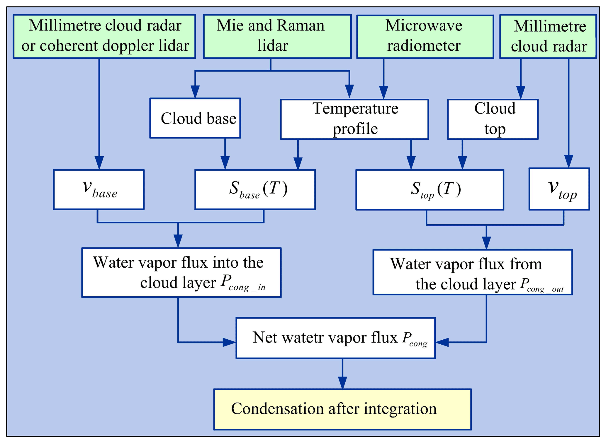
Figure 2 Technical route of remote sensing observations for atmospheric column condensate evaluation.

Although lidar and millimetre cloud radar instruments have the advantages of high spatiotemporal resolution, their detection accuracy for temperature and wind speed is affected by the system signal-to-noise ratio (SNR), which can affect the quantification accuracy of atmospheric column condensate. The determination of atmospheric column condensate depends on the water vapour flux into the cloud. According to the standard error propagation method, the uncertainty in the water vapour flux ${\mathit{\sigma }}_{p_{\mathrm{wv}}}$ depends on the input and output flux errors ${\mathit{\sigma }}_{p_{\mathrm{wv}\mathrm{\_}\mathrm{in}}}$ and ${\mathit{\sigma }}_{p_{\mathrm{wv}\mathrm{\_}\mathrm{out}}}$. These errors are determined by the uncertainty in the wind speed σ_v and the saturated water vapour density σ_S, and ${\mathit{\sigma }}_{p_{\mathrm{wv}\mathrm{\_}\mathrm{in}}}$ and ${\mathit{\sigma }}_{p_{\mathrm{wv}\mathrm{\_}\mathrm{out}}}$ can be written as Eqs. (9) and (10) on the assumption that σ_S and σ_v do not vary with time and are independent of each other.

$$\begin{array}{}\text{(9)}& {\displaystyle }{\mathit{\sigma }}_{p_{\mathrm{wv}\mathrm{\_}\mathrm{in}}}=\sqrt{{\mathit{\sigma }}_{S_{\mathrm{base}}}^{\mathrm{2}}\cdot {\stackrel{\mathrm{‾}}{v}}_{\mathrm{base}}(t{)}^{\mathrm{2}}+{\mathit{\sigma }}_{v_{\mathrm{base}}}^{\mathrm{2}}\cdot {\stackrel{\mathrm{‾}}{S}}_{\mathrm{base}}^{\mathrm{2}}(T,t)}\text{(10)}& {\displaystyle }{\mathit{\sigma }}_{p_{\mathrm{wv}\mathrm{\_}\mathrm{out}}}=\sqrt{{\mathit{\sigma }}_{S_{\mathrm{top}}}^{\mathrm{2}}\cdot {\stackrel{\mathrm{‾}}{v}}_{\mathrm{top}}(t{)}^{\mathrm{2}}+{\mathit{\sigma }}_{v_{\mathrm{top}}}^{\mathrm{2}}\cdot {\stackrel{\mathrm{‾}}{S}}_{\mathrm{top}}^{\mathrm{2}}(T,t)}\end{array}$$

The overline mean is the average of parameters in a short measurement period. The uncertainty in the saturated water vapour density depends on the temperature accuracy σ_T. The standard deviation can be obtained according to Eqs. (11) to (13):

$$\begin{array}{}\text{(11)}& {\displaystyle }{\mathit{\sigma }}_S={\displaystyle \frac{\mathrm{d}S\left(T\right)}{\mathrm{d}T}}\cdot {\mathit{\sigma }}_T,\text{(12)}& {\displaystyle \frac{\mathrm{d}S\left(T\right)}{\mathrm{d}T}}={\displaystyle \frac{\mathrm{2.17}(T+\mathrm{273.15})\cdot \frac{\mathrm{d}e\left(T\right)}{\mathrm{d}T}+\mathrm{2.17}e\left(T\right)}{(T+\mathrm{273.15}{)}^{\mathrm{2}}}},\text{(13)}& {\displaystyle }\begin{array}{rl}{\displaystyle \frac{\mathrm{d}e\left(T\right)}{\mathrm{d}T}}& ={\displaystyle \frac{\mathrm{610.8}\times \mathrm{17.27}(\mathrm{2}T+\mathrm{237.3})}{(T+\mathrm{237.3}{)}^{\mathrm{2}}}}\\ & \cdot \exp \left({\displaystyle \frac{\mathrm{17.27}T}{T+\mathrm{237.3}}}\right).\end{array}\end{array}$$

The detection uncertainty of the instantaneous atmospheric column condensate varies with the cloud base temperature. The temperature uncertainty of lidar at the cloud base ranges from 0.5 to 1 K, and the measurement uncertainty of the wind speed is lower than 0.1 m s⁻¹. Choosing spring in northern China as an example and assuming that the ground surface temperature is 15 ^∘C and the height of the cloud base is 3 km, the temperature of the cloud base ranges from approximately −3 to −4 ^∘C. The standard deviation of lidar for water vapour flux detection is approximately 0.7 g m⁻² s⁻¹ according to Eqs. (9) to (13).

5 Instrumentation

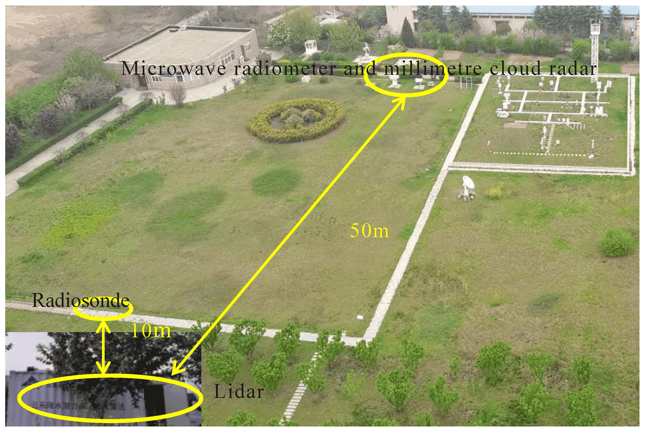
The ground-based instruments used in this study are as follows: millimetre cloud radar, which provides reflectivity and Doppler spectrum data; microwave radiometer, which provides temperature profile; and lidar, which can provide the temperature, humidity profile, particle polarisation characteristics, etc. These detection devices are installed at the Atmospheric Exploration Centre of the China Meteorological Administration. As shown in Fig. 3, the microwave radiometer and millimetre cloud radar are placed next to each other, approximately 50 m away from lidar. The launch site of the sounding balloon occurs only 10 m from lidar. Compared to the observation target, the distance between these devices is approximately negligible, so this step provides a reliable research basis for subsequent joint observation and data inversion.

Figure 3 Installation of the equipment at the observation points.

6 Remote sensing technology of the atmospheric temperature and vertical airflow velocity

6.1 Rotational Raman lidar for temperature profiles

An ultraviolet rotational–vibrational Mie–Raman lidar system was established at Xi'an University of Technology (34.233^∘ N, 108.911^∘ E) in 2019. The ultraviolet wavelength of 354.7 nm was chosen to enhance the vibrational–rotational Raman signals, as the intensity of molecular scattering is sensitive to the wavelength of the incident light. This lidar system employs a Nd:YAG pulsed laser as the light source. The output energy at a frequency-tripled wavelength of 354.7 nm is ∼ 220 mJ at a 20 Hz repetition rate with the 9 ns FWHM pulse duration. The laser beam divergence reaches approximately 0.3 mrad. The receiver is constructed using a Cassegrain telescope with a diameter of 400 mm and a focal length of 2000 mm. The collected lidar returns are coupled into a multimode fibre-optic and guided into a high-efficiency spectroscopic box. All signals were detected by photomultiplier tubes. Two pure rotational Raman signals with different temperature dependences of the central wavelengths of 352.5 and 353.9 nm were selected to retrieve atmospheric temperature profiles. A set of dichroic mirrors and narrow-band interference filters with narrow angles of incidence was utilised to construct a high-efficiency five-channel polychromator. The lidar system could detect temperatures at heights from 0.5–5 km under clear-sky or thin-cloud conditions. In addition to the temperature, the cloud base height is important. An improved differential zero-crossing method (Mao et al., 2010) was used for the retrieval of the cloud base height.

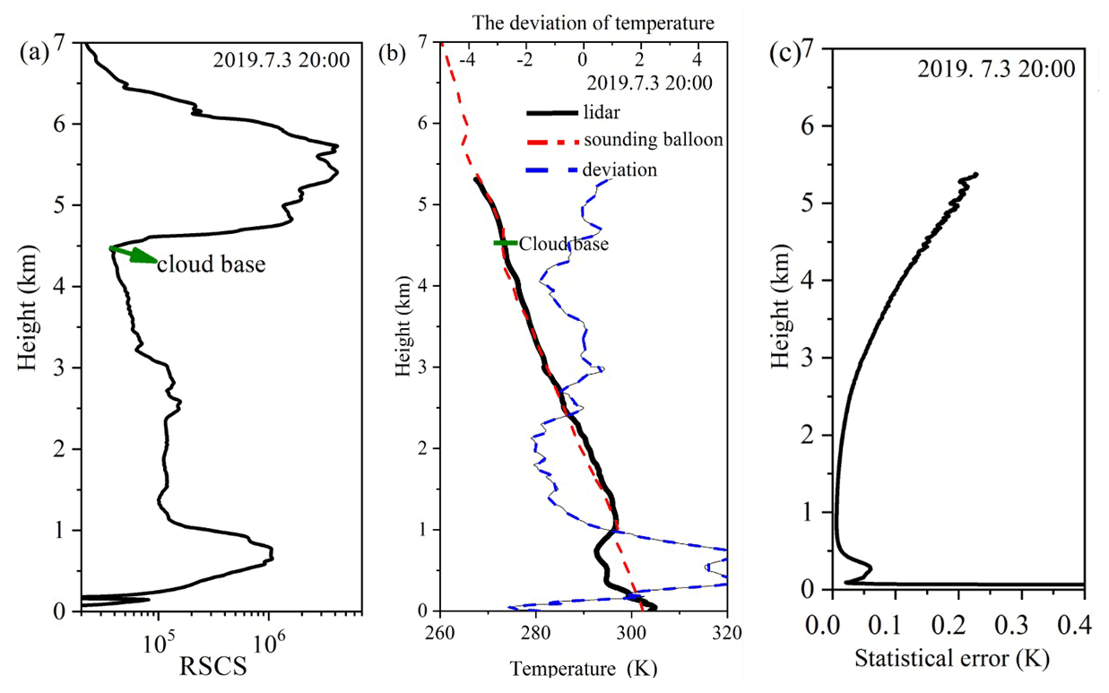
Figure 4 Mie-scattering signal (a), temperature profile (b) and statistical error (c) detected by the rotational Raman lidar.

Figure 4 shows a set of range-squared-corrected signals (RSCSs) (Fig. 4a) and temperature profile data retrieved from rotational Raman signals under cloudy weather conditions detected with lidar. The height of the cloud base was approximately 4.5 km. The figure also shows radiosonde data and the absolute deviation during the same period (Fig. 4b). Figure 4b shows the retrieved temperature data at 0.7 km from the cloud base to the inside of the cloud, and there was a good match between the lidar and radiosonde data. The absolute deviation near the cloud base was less than 1 K. Due to the influence of overlap, the temperature below 1 km exhibited a large deviation. Because this paper focuses on the temperature at the cloud base, the deviation of the base layer was not considered. Figure 4c shows the temperature statistical error calculated according to SNR of lidar. The temperature uncertainty near the cloud base was less than 0.5 K. To further estimate the reliability of the Raman lidar, we used 50 sets of temperature profiles to perform regression analysis between the lidar and radiosonde data. As shown in Fig. 5, the correlation coefficient reached 0.98 below a height of 5 km, and the root mean square error was 1.2 K.

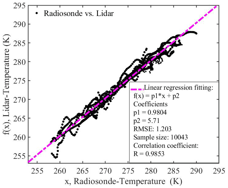
Figure 5 Regression analysis between the Raman lidar and radiosonde data and root mean square of the temperature.

6.2 Millimetre cloud radar for the vertical airflow velocity

The vertically pointing 35 GHz millimetre cloud radar (Williams et al., 2016) is often used in cloud research. The size of cloud particles is related to the natural falling velocity of cloud particles. The radial velocity measured by the vertically pointing millimetre cloud radar includes the falling velocity of cloud particles in a static atmosphere and atmospheric vertical velocity. Regarding microscale cloud particles, the natural falling speed is very low (within 2 cm s⁻¹), and the vertical motion speed of air can be 1–2 orders of magnitude larger than that of cloud particles (Kollias et al., 2001, 2011).

Figure 6 Schematic diagram of power spectrum data processing.

Both vertical air motion and particle falling speed contribute to the Doppler velocities measured by cloud radars (Gossard et al., 1996). Moreover, the spectrum of radar Doppler velocities is influenced by turbulence within the radar volume. Thus, the derivation of vertical air motions from vertically oriented cloud radar measurements is only possible under specific sets of conditions. First, with explicit knowledge of the cloud particle size distribution, a quiet-air spectrum of particle falling speeds can be computed and can then be compared to the measured radar Doppler spectrum to provide an estimate of vertical air motion (O'Connor et al., 2005). Quiet-air Doppler spectra can also be determined by deconvolving the falling speed and turbulent contributions to the measured radar Doppler spectrum. These methods rely on assumptions regarding the shape of the particle size distribution and the particle size–falling speed relationship (Gossard, 1994; Gossard et al., 1996) and/or computationally intensive inversion processes (Babb et al., 1999). If only the vertical velocity is desired, a much simpler retrieval method can be applied that only requires prior knowledge on the presence of small particles, such as liquid water cloud droplets, in the radar volume that are assumed to be tracers of clear-air motion (Gossard, 1994; Kollias et al., 2001; Shupe et al., 2007, 2008). Here, we exploit this last condition to derive vertical air velocities from cloud radar measurements. Assuming that the vertical motion of the atmosphere is uniform during millimetre cloud radar detection, the Doppler velocity from small to large corresponds with the particle size from small to large. The size distribution of supercooled liquid droplets is relatively narrow, and their spectrum can be closely approximated by a Gaussian model. The first spectral point on the left side of the power spectrum represents the signal of the smallest particle that can be detected by the radar. As shown in Fig. 6, W_air is the vertical velocity of the air.

Precise wind field measurements under rainy conditions are a challenge due to the presence of interfering signals resulting in raindrop reflections (Kollias et al., 2011). Precipitation particles often occur in cloud layers, so it is very important to distinguish the falling velocity of raindrops and the vertical airflow velocity. Under rainy conditions (Luke and Kollias, 2013; Kollias et al., 2011), the received backscattering signal contains two components, the cloud particle signal and the precipitation particle signal. Two peaks of the Doppler power spectrum can be observed if the wind and rainfall velocities differ. The vertical airflow and raindrop falling velocity can be distinguished according to the difference in their power spectra.

7 Case study of the observation of atmospheric column condensate

7.1 Joint detection of clouds with remote sensing instruments

Stratiform clouds were observed with lidar and millimetre cloud radar during the period from 8 to 9 June 2021. During this period, a weak rainfall process occurred, and clouds dissipated later. Figure 7a shows the RSCSs at 1064 nm from lidar, and Fig. 7b shows the results of the millimetre cloud radar.

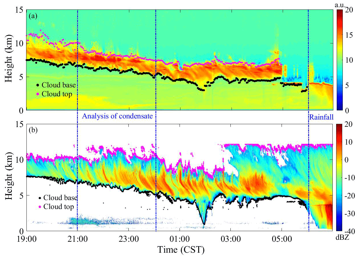
Figure 7 (a) Time–height-indicator (THI) plots of the range-squared-corrected signal (RSCS) observed by lidar at 1064 nm; (b) time–height-indicator (THI) plots of the reflectivity observed by millimetre cloud radar.

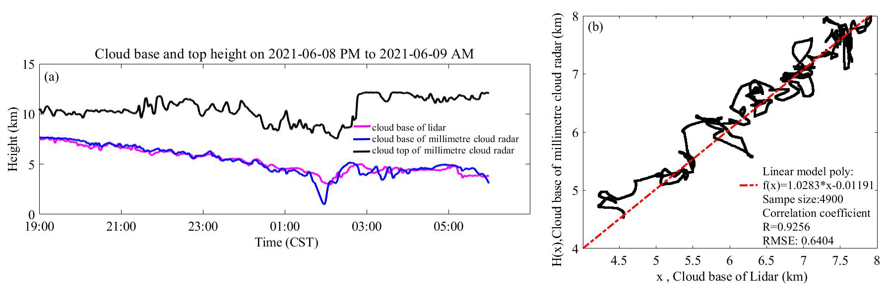
Figure 8 Cloud base heights detected by lidar and millimetre cloud radar. (a) Time series of the cloud base height, (b) correlation analysis of the cloud base height.

According to Fig. 7, the cloud layer was detected simultaneously by lidar and the millimetre cloud radar, and the cloud base height decreased from ∼ 8 to ∼ 0.5 km during the observation period. The cloud base height was maintained at approximately 5 km from 03:00 to 05:00 CST (China standard time)​​​​​​​ on 9 June 2021, while the cloud thickness increased. There was rain on 9 June 2021, but lidar could not effectively detect rainfall. However, cloud changes during rainfall were effectively observed by the millimetre cloud radar. The penetration ability of the millimetre cloud radar is greater than that of lidar. The value distribution equalisation (Zhao et al., 2014) method was used to calculate the cloud base height change detected by lidar (the black mark in Fig. 7a). Based on the millimetre cloud radar detection mechanism (Shupe et al., 2007), the cloud base and cloud top of the millimetre cloud radar were derived (Fig. 7b). The black points represent the cloud base, and the flat red points represent the cloud top. Because the penetration ability of lidar is not as good as that of the millimetre cloud radar, the height of the cloud top is subject to the detection result of the millimetre cloud radar. The values of the cloud base height detected by the two devices are shown in Fig. 8. The cloud base height and its change trend detected by the two devices exhibit a high degree of coincidence during the observation period (before rainfall). Correlation analysis was carried out. The results are shown in Fig. 8, and the correlation was 0.9256. It is verified again that these two devices provide a certain consistency in the macroscale parameters of clouds in the process of joint observation.

During the period of observation, the cloud-phase state also changes with the cloud thickness and height. Through discrimination and identification of the cloud-phase state in the observation process (Shupe et al., 2008), it was determined that the cloud-phase state was a mixed-phase state from 21:00 to 23:59 CST on 8 June 2021, and the state remained relatively stable. The base of the cloud was a liquid water area. During this detection period, the small-particle tracing method could be used to accurately obtain the W_air, which could improve the accuracy of condensate determination. During the period of 21:00–23:59 CST (it is marked with a blue dotted line in Fig. 7), the temperature and vertical velocity of the cloud boundary were detected, and the saturated water vapour density of the cloud boundary was calculated according to the temperature. The water vapour flux into the cloud during this period, that is, the maximum possible condensate, was deduced. From Figs. 7 and 8, the cloud bottom height keeps falling, indicating that water vapour is constantly replenished into the clouds and condensed water was generated. The column condensate after 23:59 CST is not calculated in this paper, mainly because the vertical velocity calculated by the minimum-particle tracing method of the millimetre cloud radar is inaccurate, which will introduce large calculation deviation.

7.2 Temperature and vertical wind velocity at the cloud base and top

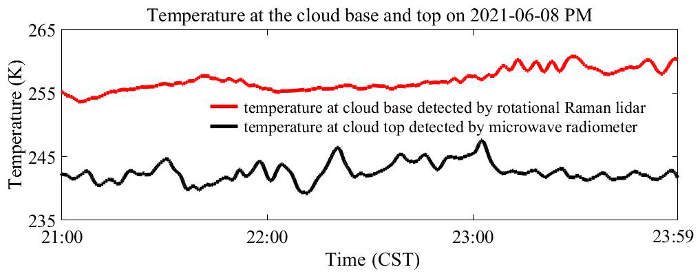
The temperature information below the cloud was retrieved according to the rotational Raman signal of lidar. Combined with the cloud base position, a time series of the cloud base temperature was obtained. The temperature at the cloud top cannot be detected by lidar. Microwave radiometer data were chosen as a supplement for temperature determination. The results of the microwave radiometer were validated against sounding balloon data, and the temperature deviation of the microwave radiometer was less than 2 K. A time series of the cloud top temperature was also derived. The temperature results at the cloud base and top (8 June 2021 21:00–23:59 CST) are shown in Fig. 9.

Figure 9 Time series of the temperature at the cloud base and top.

Figure 10 Time series of the air vertical motion velocity at the cloud base and top.

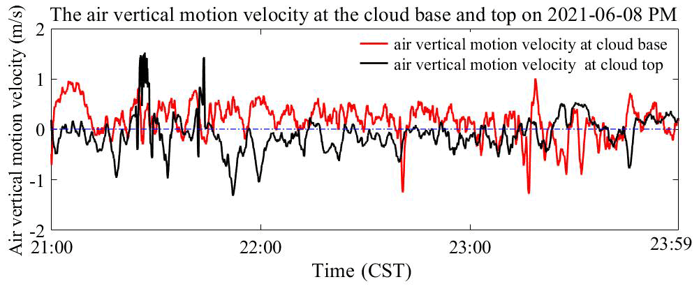
The power spectrum data of the millimetre cloud radar from 21:00 to 23:59 CST on 8 June 2021, were analysed, and the air vertical motion velocity at the cloud base and cloud top (positive upward and negative downward) was obtained via the small-particle tracing method described above (Sect. 6.2). The results are shown in Fig. 10. The calculated atmospheric vertical velocity value is relatively consistent with Shupe et al. (2007). Figure 10 shows that mainly updraft occurred at the cloud base. The updraft and downdraft processes at the cloud top were staggered, but mainly the downdraft process, which is also in line with the phenomenon of cloud top height decline.

7.3 Results of atmospheric column condensate

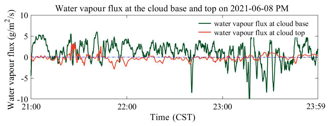
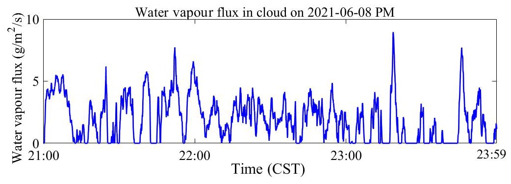
The water vapour flux was calculated according to Eqs. (2)–(8). As shown in Fig. 10, the cloud top temperature was approximately 12–15 ^∘C lower than the cloud base temperature. Therefore, it could be considered that the water vapour remaining in the cloud could condense to a large extent. The rising air at the cloud top brings water vapour out, reducing condensate content in the cloud. Figure 11 shows the water vapour flux through the cloud base and cloud top. In this observation, both water vapour entering the cloud base and water vapour leaving the cloud top occur. The water vapour flux entering the cloud base minus the water vapour flux leaving the cloud top is the value remaining in the cloud layer, which could be considered the maximum possible condensate flux. If the water vapour flux is positive, the cloud is constantly generating and developing, and if the flux is negative, the cloud is dissipating. Figure 12 shows the instantaneous water vapour flux remaining in the cloud layers.

Figure 11 Time series of the water vapour flux at the cloud base and top.

Figure 12 Instantaneous water vapour flux remaining in the cloud layer.

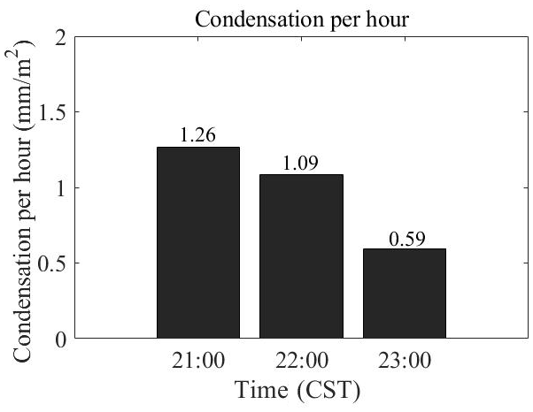
The atmospheric column condensate could be obtained by integrating the instantaneous water vapour flux. Figure 13 shows the hourly condensate during the observation period. As shown in Fig. 11, updraft at the cloud top was very limited, so it can be deduced that the water vapour entering the cloud basically remained in the cloud. According to Eq. (5), the condensate over the period from 21:00 to 23:59 CST was integrated, and it could be found that the total number of the maximum possible condensate in the atmosphere during this period was approximately 88.2 g m⁻² (2.94 mm m⁻²). The water condensed during this period provided resources for the incoming rainfall at 06:00 CST on 9 June 2021. Therefore, the detection and derived results are in good agreement with the changes in weather and clouds on this day.

Figure 13 Hourly condensate during the observation period.

8 Results and discussion

It is very difficult to directly measure atmospheric column condensate. According to the characteristics of different remote sensing equipment, the condensate content can be deduced by measuring meteorological parameters near and inside the cloud deck. This paper presents a remote sensing method for atmospheric column condensate detection by using lidar, millimetre cloud radar and microwave radiometer instruments. A detailed detection scheme and data calculation method are given. A precipitation process was observed, and atmospheric column condensate was obtained by active and passive instruments. In this method, it is considered that the water vapour remaining in the cloud can condense, which is an ideal assumption. In fact, some of the water vapour entering the cloud evaporates or exits the cloud boundary, which can lead to a reduction in the condensate. These effects are not considered in this paper. We provide the maximum possible atmospheric column condensate. Therefore, the derived condensate should be larger than the actual value. Nevertheless, the method proposed in this paper remains valuable. The method proposed in this paper only uses observation data at one point to represent the results throughout the whole region, which is reasonable for horizontally uniform stratiform clouds. Regarding clouds with strong convection, it is more effective to use multipoint network observation data.

Stratiform clouds often appear in northern China and are the main targets of artificial weather modification. The vertical airflow velocity under stratiform clouds is low and should be obtained with high-precision detection equipment. Lidar is an effective instrument to obtain high-precision wind speed and temperature data below clouds. Precipitation involves a complex weather system that can be divided into two categories: convective precipitation and systematic precipitation. Convective precipitation generally covers a small range. The horizontal scale of convective clouds is on the order of 100 km, and the water vapour supply is mainly provided by the rise of air near the ground. Updraft before precipitation can be measured with the millimetre cloud radar or lidar to obtain the potential precipitation, namely, the total amount of cloud water in a certain area and a certain period of time. After the beginning of precipitation, if the precipitation is very low, a lidar instrument can also detect the temperature and updraft in the precipitation area, but when there is heavy precipitation, lidar cannot obtain effective data. Systematic precipitation is complex, and a multilayer cloud structure can emerge. Lidar instruments usually cannot penetrate multilayer clouds, and these devices are only suitable for the detection of the base of single-layer clouds. In terms of multilayer clouds, it is necessary to use the millimetre cloud radar to detect the vertical air velocity in multilayer clouds and a microwave radiometer to detect the temperature in clouds.

The assessment of CWRs in an area requires long-term statistical results, which necessitate long-term continuous remote sensing observations. This paper provides a detection method for atmospheric column condensates and a scientific observation case. More cloud observation results will be carried out in the future for the assessment of CWRs.