the Creative Commons Attribution 4.0 License.
the Creative Commons Attribution 4.0 License.
 | 14 Jun 2022
ERUO: a spectral processing routine for the Micro Rain Radar PRO (MRR-PRO)
Alfonso Ferrone
Anne-Claire Billault-Roux
The Micro Rain Radar PRO (MRR-PRO) is a K-band Doppler weather radar, using frequency-modulated continuous-wave (FMCW) signals, developed by Metek Meteorologische Messtechnik GmbH (Metek) as a successor to the MRR-2. Benefiting from four datasets collected during two field campaigns in Antarctica and Switzerland, we developed a processing library for snowfall measurements named ERUO (Enhancement and Reconstruction of the spectrUm for the MRR-PRO), with a twofold objective. Firstly, the proposed method addresses a series of issues plaguing the radar variables, including interference lines and power drops at the extremes of the Doppler spectrum. Secondly, the algorithm aims to improve the quality of the final variables by lowering the minimum detectable equivalent attenuated reflectivity factor and extending the valid Doppler velocity range through dealiasing. The performance of the algorithm has been tested against the measurements of a co-located W-band Doppler radar. Information from a close-by X-band Doppler dual-polarization radar has been used to exclude unsuitable radar volumes from the comparison. Particular attention has been dedicated to verifying the estimation of the meteorological signal in the spectra covered by interferences.
- Article
(11175 KB) - Full-text XML
- BibTeX
- EndNote


While most of the densely populated areas of the planet benefit from the coverage by operational radar networks (Saltikoff et al., 2019), remote locations are often scarcely monitored. In some regions of the Arctic, Antarctica, or high mountains, snowfall can be the dominant precipitation type. In those locations, measurements of precipitation, and snowfall in particular, are hindered by technical and logistical difficulties. In the last decades, however, field campaigns involving the deployment of small radars in such locations have been becoming more common. One notable example is the Micro Rain Radar (MRR-2) (Klugmann et al., 1996), developed by Metek Meteorologische Messtechnik GmbH (Metek): a K-band (24 GHz) Doppler weather radar, using frequency-modulated continuous-wave (FMCW) signals. Multi-year datasets of its measurements are already available in several locations in Antarctica (Gorodetskaya et al., 2015; Grazioli et al., 2017), proving its suitability for deployment in hostile environments. Its potential for snowfall measurements has already been unlocked by the IMProToo algorithm (Maahn and Kollias, 2012), an alternative processing technique for the raw MRR-2 spectra. By using an improved noise removal algorithm, their method can detect fainter meteorological signals, while the dealiasing allows for the recording of velocity values beyond the Nyquist velocity range, even though this eventuality is arguably rare in snowfall conditions. A different method, based on an alternative processing and dealiasing algorithm, has been proposed by Garcia-Benadi et al. (2020). Their technique also provides information on the dominant hydrometeor type in the observed radar values and attempts to distinguish between precipitation types. A similar attempt, using two different classification algorithms, has also later been proposed by Foth et al. (2021).
The successor of the MRR-2 is the Micro Rain Radar PRO (MRR-PRO): also developed by Metek, it is a K-band Doppler FMCW weather radar. Given its low power consumption, small size, and relatively affordable cost, it is an ideal instrument for deployment in remote locations. Its usage for precipitation measurements has already been attested in the Antarctic Peninsula (Pishniak et al., 2021) and on the Antarctic coast (Alexander, 2019). However, to the best of our knowledge, no alternative processing procedures specific to this radar have yet been proposed to the scientific community. Theoretically, some of the processing algorithms designed for the MRR-2 may be readapted for the MRR-PRO. The first, arguably minor, problem that may be encountered in following this approach is differences in file type and the measurement configuration. In particular, some of the MRR-PRO configurable and fixed parameters differ from the ones of its predecessor, and any algorithms designed for the latter may need to be retuned.
The Environmental Remote Sensing Laboratory at EPFL had access to three of these radars, and in the last year, they have been used for snowfall measurements in Switzerland and Antarctica. In all the datasets collected, we observed the presence of strong and semi-fixed signals, persisting for most of the duration of the campaign, at a few radar-dependent range gates. Examples from the three MRR-PRO systems are shown in Fig. 1. In the four datasets used in the analysis, they often appear in the upper part of the profile, at more than 3 km of altitude above the radar. Lower altitudes can also be affected, as illustrated by the line at approximately 1 km of height in Fig. 1e. These signals appear in all radar variables, and they originate from spurious peaks in the raw spectra, spanning either a few or all the spectral line numbers. They appear even when the radar is deployed on the Antarctic plateau, hundreds of meters away from any tall orography and not surrounded by any structure taller than the MRR-PRO itself. An example of such behavior can be seen in Fig. 1c. To simplify the following discussion, we will hereafter refer to these anomalous signals as interference lines. We suspect their origin to be a kind of interference internal to the radar, but we could not precisely identify it, and their technical investigation is beyond the scope of this study. These interference lines and some other issues with the radar data, described later throughout the paper, are the second (and main) reason that we decided not to readapt the MRR-2 algorithms to the MRR-PRO. These issues in the measurements need to be addressed by a new method designed to remove them and specifically tune them to the MRR-PRO.
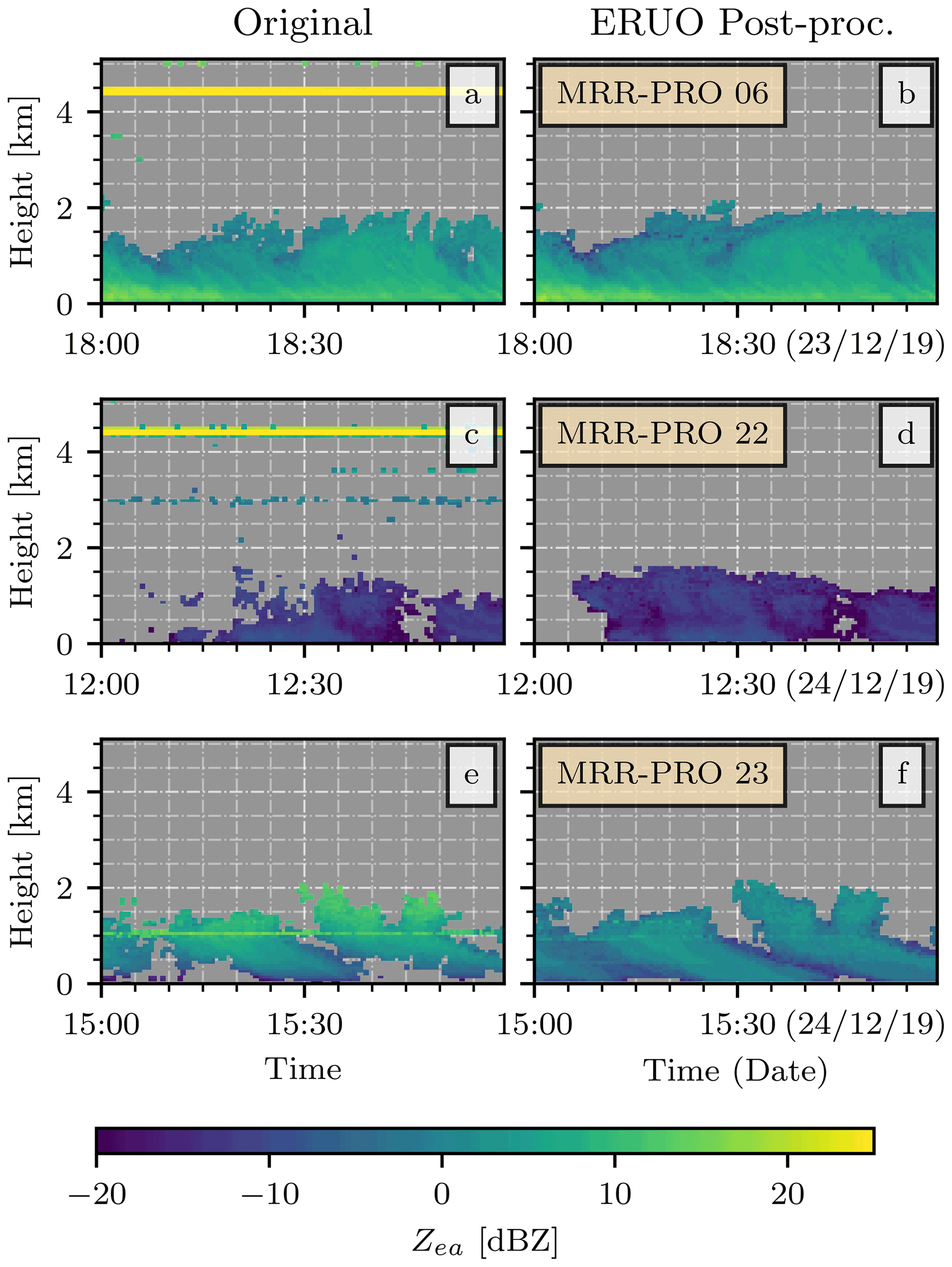
Figure 1Examples of attenuated equivalent reflectivity factor (Zea) from MRR-PRO files. Panels (a), (c), and (e) show the original, unprocessed products. Panels (b), (d), and (f) show the final ERUO products. Each row displays an example from a different radar: panels (a) and (b) for the MRR-PRO 06, panels (c) and (d) for the MRR-PRO 22, and panels (e) and (f) for the MRR-PRO 23. All y axes display the height above the first range gate of the MRR-PRO.
Therefore, this study presents a new processing algorithm for the MRR-PRO raw data, targeted at snowfall measurements, with a twofold objective. Firstly, for a correct interpretation of the data, these interference lines need to be eliminated from all the variables. Thus, our method attempts to remove the spurious peaks from the raw spectra, reconstructing a clean copy and using it as a starting point for the processing. Similarly, other issues such as the power drop observed at the extremes of the Doppler velocity range are also addressed by the ERUO library. The second objective is an overall improvement of the quality of snowfall measurements: a different approach in the noise floor estimation ensures a better sensitivity, while the dealiasing allows for an extended range of detectable Doppler velocities. Snowfall has been chosen as the main target of our library because its measurements can benefit significantly from improvements in sensitivity and because the MRR-PRO files already contain a plethora of information specific to rain, thanks to the dedicated algorithm developed by Metek. Examples of the final results of the ERUO library are shown in Fig. 1b, d, and f.
The method proposed in this study is named ERUO: Enhancement and Reconstruction of the spectrUm for the MRR-PRO. This acronym has also been chosen for the meaning of the word “eruo” in classical Latin: depending on the context, it may literally be translated with the verb “to dig”, and, in figurative speech, it may be interpreted as “to bring out”. In a sense, our algorithm digs into the spectrum, extracting the meteorological signal from below the interference lines covering it.
All the data and the additional instruments used in the analysis are presented in Sect. 2. The method is described in detail in Sect. 3, which is in turn divided into three subsections, each dedicated to one of the three main stages of the algorithm. The validation of the proposed method is in Sect. 4, by comparing the output variables with the original MRR-PRO products and with the measurements of a second radar. A subsection has been dedicated to evaluating the spectrum reconstruction, which is one of the innovative aspects of the proposed method. Finally, Sect. 5 contains our conclusions on the performance of the algorithm and its limitations.
2.1 The MRR-PRO
The first three datasets used in this study have been collected by three MRR-PRO deployed in the vicinity of the research base Princess Elisabeth Antarctica (PEA) during the austral summer of 2019/2020. The radars have been installed at three different locations, approximately 7 and 17 km apart from each other. The sites are placed across the mountains south of the base to capture the evolution of precipitation systems at different stages of their interaction with the complex orography. To better distinguish between the three instruments in the following discussion, we will refer to each system by its serial number: MRR-PRO 06, MRR-PRO 22, and MRR-PRO 23.
The fourth dataset is the result of a measurement campaign that took place in La Chaux-de-Fonds, in the Swiss Jura, during the boreal winter of 2020/2021. The campaign was conducted in the framework of the Horizon 2020 ICE GENESIS project (ICE GENESIS Consortium, 2021), a collaboration of 36 partners from 10 countries, whose aim is to improve the representation of snowfall in the perspective of aircraft safety. One of the radars used in PEA, the MRR-PRO 23, was deployed at the airport of the city. We will refer to this instrument as MRR-PRO ICE-GENESIS (shortened to ICE GENESIS in figures) when discussing matters pertaining to this campaign to avoid confusion in the following text.
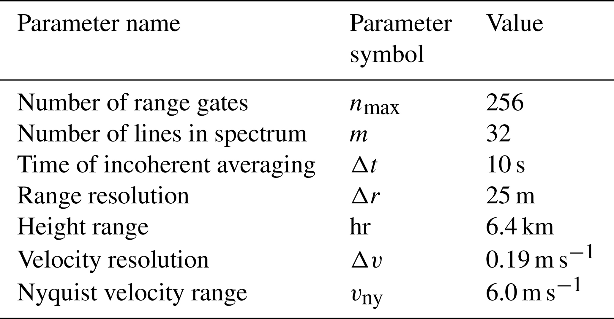
The MRR-PRO allows for a higher degree of customization in the measurement settings respect to its predecessor, the MRR-2. In both campaigns, all the MRR-PRO have been configured with the same parameters, listed in Table 1. Due to constraints in the maximum allowed power consumption on-site, the antenna heating had to be turned off for the whole deployment period.
Table 1Measurement setup of all the MRR-PRO systems used in the study. A symbol has been associated with each parameter, to ease the referencing in the text.
For each dataset, the variables saved by the radars and used in the study are as follows:
-
, the raw spectrum, dependent on the time (t), spectral line number (), and range gate number () and measured in logarithmic spectral units (), proportional to the return power;
-
Zea(t,n), the attenuated equivalent reflectivity factor, expressed in decibels relative to Z (dBZ);
-
V(t,n), the mean Doppler radial velocity, in ms−1;
-
SW(t,n), the spectral width, also in ms−1;
-
SNR(t,n), the signal-to-noise ratio, in decibels (dB).
While variables collected by a specific radar will be written in bold roman font, as per convention when dealing with matrices, the same symbol or acronym will be used in italic to denote the respective variable in general, without referring to a specific instance of it.
The MRR-PRO needs to be explicitly configured to save the raw spectrum rather than the reflectivity spectrum. ERUO is designed to function only with the former, even though we expect that only minor modifications would be needed to allow for the support of the latter. In theory, it may be possible to convert the spectrum reflectivity back into raw spectrum and use the data directly as input for ERUO. However, any faint signal below the noise level used for generating the original files will not be recoverable in this way.
The variables listed above are accompanied by a set of auxiliary quantities: TF(n), the transfer function, which compensates for a change in receiver sensitivity related to the changing frequency of FMCW radars, and c, the radar calibration constant used in the conversion from spectral density to spectral reflectivity. The usage of both variables is described in Sect. 3.2.4.
2.2 WProf
During the ICE GENESIS campaign, a vertically pointing W-band (94 GHz) Doppler cloud radar (Küchler et al., 2017), hereafter referred to as WProf, was also deployed at the airport of La Chaux-de-Fonds, approximately 10 m away from the MRR-PRO. This radar, officially known by the commercial name RPG-FMCW-94-SP, is developed by Radiometer Physics GmbH (RPG). Its remarkable sensitivity, combined with the high resolution resulting from the usage of FMCW signals, makes it the perfect reference for comparing the results of our algorithm later in this study.
Table 2Measurements setup of WProf during the ICE GENESIS campaign.
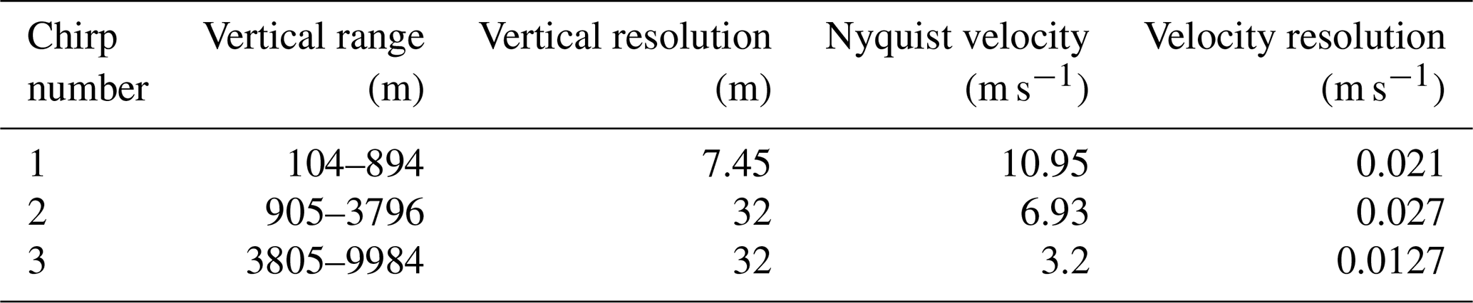
This instrument allows for a high degree of flexibility when deciding the configuration used for the data acquisition. We decided to use a chirp table divided into three stages, detailed in Table 2. Only a subset of the variables recorded by the instrument will be used in this study: , VW(t,n), and SNRW(t,n). Each quantity is denoted by the same acronym as the MRR-PRO case, while the superscript W is used to distinguish the instrument that collected them.
2.3 MXPol
The last radar playing a role in this study is an X-band (9.41 GHz) scanning Doppler dual-polarization weather radar (MXPol), developed by Prosensing (Schneebeli et al., 2013). The instrument was installed about 4.8 km away from the airport of La Chaux-de-Fonds during the ICE GENESIS campaign.
One of the scan types performed by this radar was a range height indicator (RHI) oriented towards the location of the MRR-PRO and WProf. Thanks to the dual-polarization nature of the measurements, we have access to an estimate of the hydrometeor types present in the observed volumes, computed using the classification described in Besic et al. (2016) and refined using the demixing algorithm described in Besic et al. (2018). The information on the hydrometeor population above the airport site is the only product of MXPol used in this study.
This section presents the procedure followed by ERUO to process the raw spectra collected by the MRR-PRO. A schematic representation of it can be seen in Fig. 2. The algorithm and its description are divided into three stages: preprocessing, processing, and post-processing, each described in a dedicated subsection below.
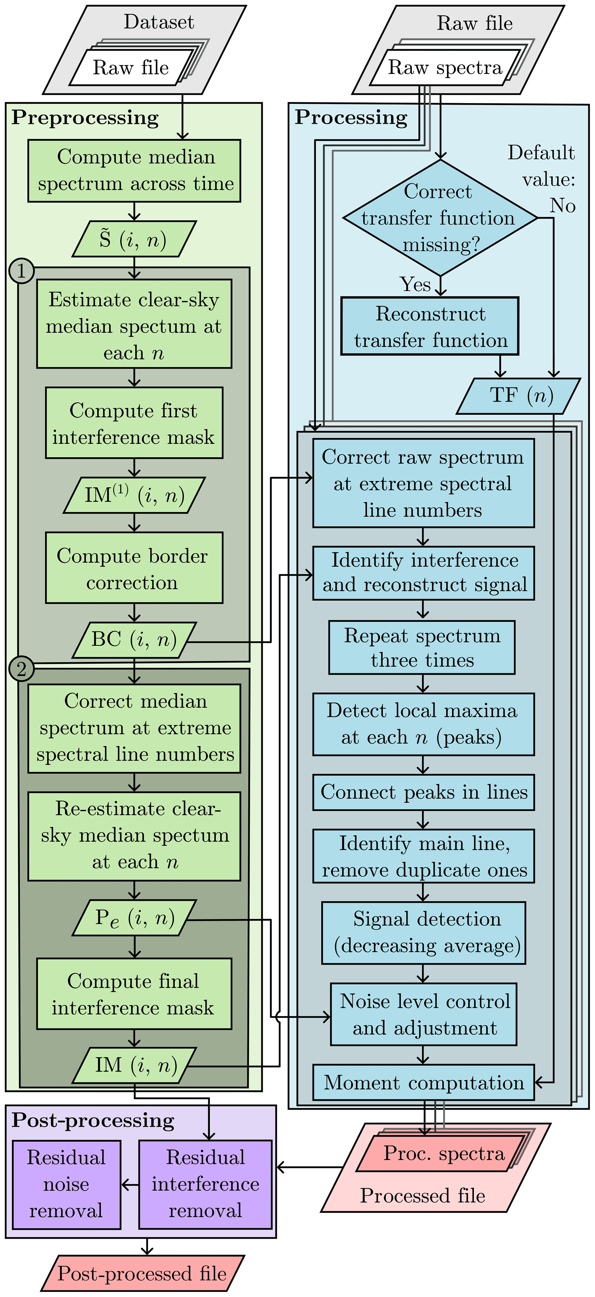
Figure 2Flowchart of the ERUO algorithm. Rhomboid shapes indicate inputs (white background) and outputs (red background), while rectangles indicate processing steps. The numbers 1 and 2 at the top-left corner of the two darker green boxes inside the preprocessing denote the two iterations described in Appendix A.
3.1 Preprocessing
The preprocessing aims to identify regions in the spectra that are systematically affected by artifacts and to produce a series of products to assist in the processing of the data files. This stage of the algorithm uses the information contained in a whole dataset, collected from a single continuous deployment of the MRR-PRO, to compute three products:
-
The interference mask, IM(i,n), highlights the regions of the raw spectra of the campaign likely affected by interference.
-
The border correction, BC(i,n), is a spectral density offset used to compensate for the drop in the raw spectra values observed at i close to 1 or m. This drop is caused by the filtering performed by the algorithm of Metek, as described for the MRR-2 by Maahn and Kollias (2012). This behavior is visible in both precipitation and clear-sky measurements;
-
The signal-free raw spectrum profile estimate, Pe(n), is the typical return recorded in each range gate during ideal clear-sky conditions, mainly due to the thermal noise of the receiver.
The procedure starts by loading all the raw spectra available in the dataset and concatenating them along the temporal axis. The resulting single 3-dimensional (t, i, n) matrix enables the analysis of the typical power return at each range gate. From this matrix, the algorithm extracts the 2-dimensional (i, n) median raw spectrum across all time steps, referred to as .
In all the four datasets presented in Sect. 2.1, no couple (i,n) experiences precipitation for more than 50 % of the duration of the campaign. Due to this relative scarcity of precipitation, the usage of the quantile 0.5 (median) to compute is an adequate choice to isolate the non-meteorological background. If the ERUO algorithm is applied to datasets with a higher frequency of precipitation, peaks associated with the meteorological signals would likely be visible in . In this case, the preprocessing can be executed using only a subset of clear-sky measurements, spread as much as possible throughout the whole time series.
A set of characteristics recurrent across the median MRR-PRO spectra of the four available datasets can be identified. First of all, the dependence of the median power on the range gate number follows the same pattern: after a sharp rise in the lowest gates, the power level briefly plateaus before starting a consistent descent that continues up to the last range gate. The exact position of the range gate in which the transition in trend happens may vary between MRR-PRO and campaigns. Another behavior consistently present in the matrix is the drop in raw spectrum observed for i close to 1 or m. Usually, this drop is fainter than other features, such as marked precipitation signal. Therefore it is extremely important to make sure that has been computed over a campaign with a relatively low frequency of precipitation (such as the ones used for this study) or over a subset of clear-sky measurements collected throughout the campaign. Finally, peaks of different sizes and prominence may appear in several locations across the median spectrum. These peaks generate the interference lines in the final MRR-PRO products. Given the presence of these anomalies in both clear-sky and precipitation measurements, their signature is visible in the temporal median of , as shown in Fig. 3. These peaks can be divided into two categories:
-
Isolated peaks occupy only a handful of spectral lines and range gates, appearing as circular or oval shape when plotting versus both n and i. An example of this type of interference can be observed in Fig. 3a, around the coordinates ;
-
Lines cover the whole i axis, from i=1 to i=m, and span only a few range gates. Figure 3b shows their typical appearance, with a particularly noticeable line in the ICE GENESIS dataset visible around n=60.
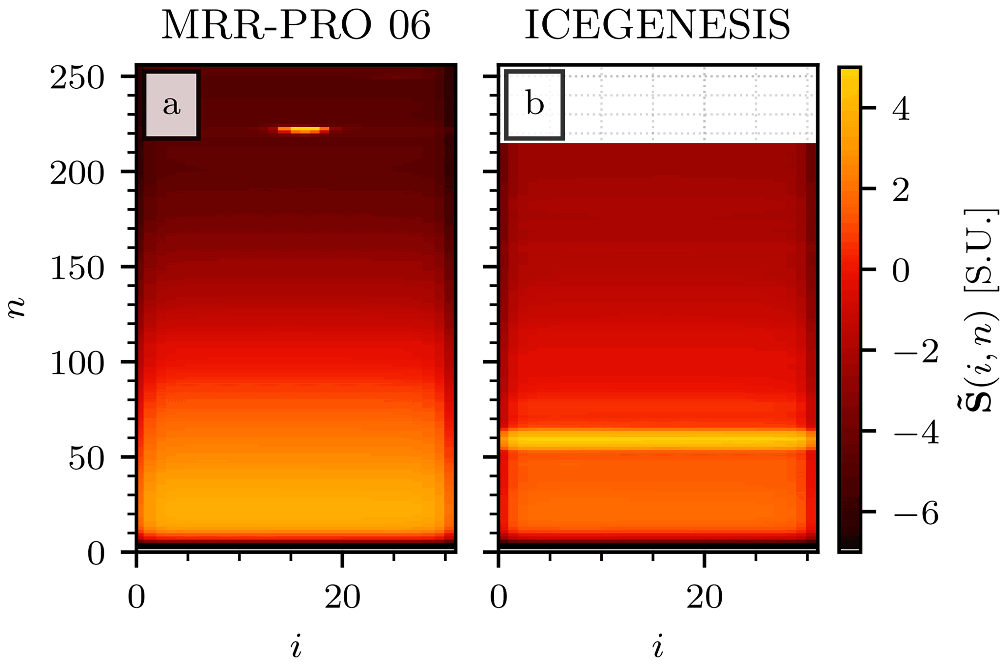
Figure 3The matrices for the MRR-PRO 06 (a) and ICE GENESIS (b) datasets. The MRR-PRO 23 did not record any data above n=215 during the deployment at La Chaux-de-Fonds, resulting in the missing section of the matrix visible in the top part of panel (b).
Each of these observations plays a role in the preprocessing, allowing for the use of the matrix as the basis from which the three products of this section will be derived. From this point onward, the algorithm continues following a two-step, quasi-iterative procedure. The technical details of the two iterations are provided in Appendix A.
3.2 Processing
Following the preprocessing steps, which compute averaged quantities for an entire dataset, this section describes how ERUO processes a single MRR-PRO file. The raw spectra stored in it constitute the starting point for the computation of a set of radar variables: , V(Proc)(t,n), SW(Proc)(t,n), and SNR(Proc)(t,n). These quantities are stored in the processed file, created at the end of the processing.
As schematized in Fig. 2, the processing can be seen as a series of short operations performed for each raw spectrum. These steps are detailed separately in the next subsections, following the same order as their appearance in the library. This list of operations may be preceded by the reconstruction of the transfer function. The latter is optional and turned off in the default configuration; therefore it is discussed separately in Appendix B.
3.2.1 Spectrum reconstruction
The first step of the spectrum-by-spectrum processing can be considered the most delicate one in the whole ERUO library. As mentioned before, removing interference lines from the final products is among the topmost priority of the ERUO routine. Their manifestations in the raw spectrum sometimes hide the meteorological signal. During precipitation, interference lines can artificially increase the amplitude of the recorded signal at the affected locations. This may result in the overestimation of Zea and, possibly, alterations of V and SW, depending on the particular shape of the interference. Additionally, in clear-sky conditions, these peaks and lines generate anomalies that are recognized as signal by standard techniques such as the one proposed by Hildebrand and Sekhon (1974). Therefore they often result in false positives of detected precipitation. ERUO intervenes by identifying the regions of each of the spectra likely affected by interference, masking parts of them, and reconstructing the masked regions using information from their surroundings by performing a kernel-based interpolation.
For each time step tj of the input file, the process starts by loading the raw spectra and summing BC(i,n) to it, obtaining the corrected raw spectra, . An ideal clear-sky guess of the power return is defined, similarly to the preprocessing case, by repeating m times along a new dimension the profile Pe(n), obtaining . This matrix is used to compute the power anomaly, defined as . The first guess of the regions of this matrix affected by interference is obtained by selecting the couples (i,n), where and S.U. The chosen threshold is significantly larger than the one used as minimum prominence for the signal detection to avoid creating vast regions of masked values. The aim of this reconstruction is the removal of the most noticeable interferences, which are usually associated with peaks taller than the minimum detectable prominence threshold. Moreover, the interpolation behind the spectrum reconstruction performs better on smaller masked areas. Therefore, this choice of threshold suits the objective, while smaller, leftover interference is easily eliminated by the post-processing.
This first guess can be seen as a collection of a few contiguous regions of masked (i,n) couples. Among those regions, only the ones that satisfy one of two conditions are kept (set to 1) in the mask:
-
The masked section is an isolated peak. In practice, for fewer than five couples (i,n) in the surroundings of the current masked region. The surrounding area, in this case, is computed by dilating twice the current contiguous masked region.
-
For some of the affected n, the masked region covers at least 80 % of the interval . This behavior may indicate the presence of an interference spanning all spectral line numbers, extreme folding of the meteorological signal, or particularly wide spectra, such as the ones recorded in presence of strong turbulence.
The set of masked regions obtained from the rules above is further refined. At each range gate number, the entry (i,n) with the highest value of A(i,n) is unmasked if strong anomalies are detected immediately above or below the region. This condition allows for the preservation of the position and intensity of the maximum return power at each rage gate, constraining the interpolation. In practical terms, the algorithm first checks if for at least one entry (i,n) within the masked region. The second control is on the existence of locations (i,n) satisfying the same condition in (at least) three of the five closest range gates below or above the masked region. If the median i coordinate of these peaks differs from the i coordinate of the maximum peak of A(i,n) within the masked region by 5 or less, the algorithm proceeds with the unmasking of the location of the largest anomaly at each range gate.
The matrix A(i,n) is copied, and, in this copy, all the previously masked regions are substituted by the “Not a Number” (NaN) value. These missing regions are reconstructed by replacing the NaN values with a kernel-weighted interpolation from their neighbors. The technical implementation of the interpolation and replacement of invalid values is the one provided by the function “astropy.convolution.interpolate_replace_nans” from the Python3 library Astropy (Astropy Collaboration et al., 2013, 2018). The kernel type used in the procedure is a Gaussian one. Its combination of standard deviation and kernel size has been chosen for its ability to capture the typical shape of the meteorological signal observed in the four datasets.
In particular, the kernel standard deviation has been fixed to 1 along the i axis. A higher value causes an artificial broadening of the reconstructed peaks compared to the precipitation signal directly above and below. On the n axis, the kernel needs to be large enough to contain non-NaN values at both its extremes to perform a meaningful interpolation. To satisfy this condition, the standard deviation size along this axis is set equal to the number of consecutive range gates containing at least one NaN divided by a scaling factor, set by default to 3. Along both axes, the kernel size is set equal to 8 times the standard deviation. Finally, an accurate reconstruction of the A(i,n) in the lowest gates, especially at the extremes of the i axis, cannot be consistently achieved with this method. Therefore, the first 15 range gates are excluded from the whole procedure.
Given the importance of this first step of the ERUO processing, its validation is presented separately in Sect. 4.3. The section includes a visual representation of both the masking of the interference and the final reconstructed product.
3.2.2 Peak detection and dealiasing
The reconstructed anomaly is added back to the baseline clear-sky return, , and it is converted to linear units. An instance of this matrix, computed for the MRR-PRO 06 dataset, can be seen in Fig. 4a. Two copies of the raw spectrum in linear units are created. The first is lowered by one range gate across the n axis, while the second is lifted by one range gate because aliasing in FMCW systems contaminates the adjacent range gates. These two copies are each attached before and after the raw spectrum along the i axis, whose limits become . The resulting matrix is denoted by , and its units are the linear spectral units, s.u. Figure 4b exemplifies the enlarged matrix. The triplication of the spectrum performed in this way is analogous to the one described for the MRR-2 by Maahn and Kollias (2012) for dealiasing purposes.
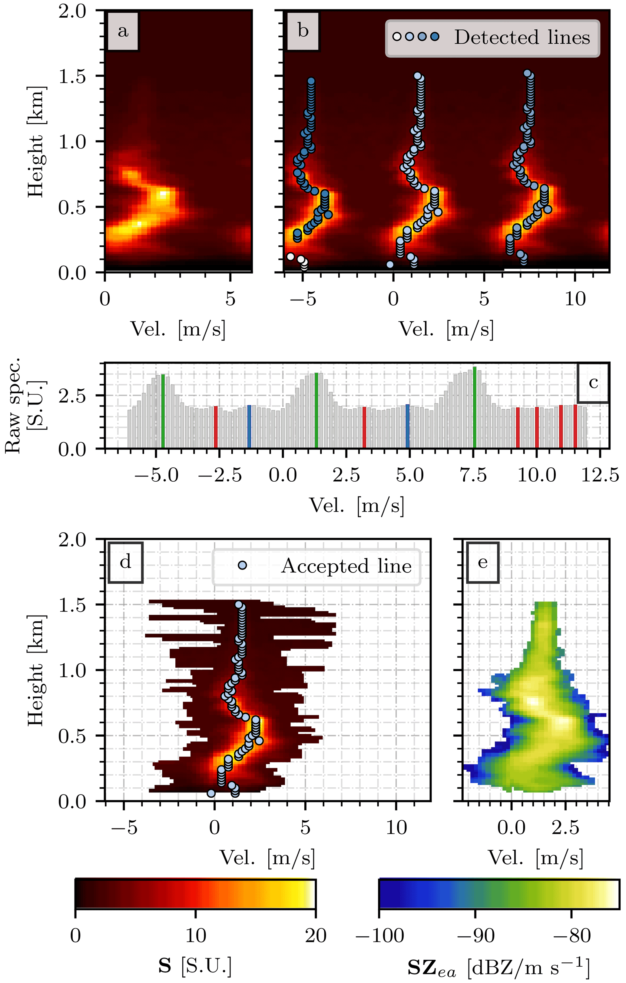
Figure 4Key steps of the processing. Using the raw spectra recorded on 18 December 2021, at 03:07:30 UTC by the MRR-PRO 06 as the starting point, panel (a) shows the result of the spectrum reconstruction and the correction at the extreme Doppler velocities. Panel (b) displays the local maxima identified at each range gate, connected in lines. Panel (c) shows the intermediate steps in the peak detection for n=50. The gray bars represent the raw spectrum, the red ones are the entries identified as peaks but rejected by the prominence threshold, the blue ones are peaks rejected by the relative prominence threshold, and the green ones are the accepted ones. Panel (d) displays the intervals of m entries selected around each peak in the main line. Finally, panel (e) illustrates the product of the signal identification and conversion in spectral reflectivity. The maximum height has been limited to 2.0 km since no precipitation was recorded above this altitude. The color bar at the bottom left refers to panel (a), (b), and (d), while the one on the right refers to panel (e).
At each range gate number, the algorithm identifies all local maxima in the spectrum. The library imposes an optional limit to the maximum number of peaks detectable at each range gate to reduce the computation time. This limit is set by default to six. If the highest maxima (usually three) have a prominence of at least 0.2 , they are saved in the list of possible signal peaks. Note that features are usually found in sets of three, given the three repetitions of the original spectrum along the m axis. Secondary maxima are also saved but only if their prominence is at least 25 % of the main ones. While the absolute threshold is kept purposefully low to detect even the faintest traces of precipitation signal, the relative one avoids the proliferation of false positives.
Figure 4c provides an example of peak detection for a spectrum collected by the MRR-PRO 06. The peaks with the highest prominence are highlighted in green, while the ones eliminated by the absolute and relative prominence threshold are displayed in red and blue, respectively. In the example, the blue peaks would have been (barely) acceptable if there were no higher ones in the spectrum. This approach allows for signals as low as the blue ones of Fig. 4c to be detected if no taller peak exists, while at the same time preventing them from interfering with the next step when a stronger signal is identified. Even though in this example only a single peak is detected for each repetition of the spectrum, it is entirely possible to retain multiple peaks in the case of multi-modality.
Once all the (i,n) coordinates of the peaks are identified, the algorithm attempts to connect them in vertical lines. For each candidate peak, the algorithm looks in a window of 5 along the n axis and 10 on the i axis around its coordinate. If another peak falls in this window, the two are connected in a line, and the procedure continues by trying to connect more peaks to the same line. Each peak can belong only to one line, each line can contain only a single peak per range gate, and multiple lines can occupy the same n (for example, in the case of bimodality in the spectrum). If multiple peaks fall in the same window, the choice always favors the one in the closest range gate, using the distance along the i axis as a secondary decision parameter. Following with the example of Fig. 4, four lines have been detected in this specific case, and they have been superimposed on in Fig. 4b.
Once the lines have been determined, the ones with fewer than three elements are excluded from the analysis. Among the remaining ones, the algorithm tries to exclude the duplicate ones caused by the three repetitions of the original spectrum. Couples of lines whose median difference along the i axis is close to m (the tolerance is 1 m s−1, converted in spectral line numbers) are flagged as duplicates. Among these couples, the algorithm keeps the line whose upper half is closer, in median, to i=0. This operation per se does not count as full dealiasing. However, given the focus of ERUO on snow and the usual slow fall speed of solid hydrometeors, especially in the upper part of the precipitation systems, this choice results in a reasonably good handling of many of the aliasing cases of our four datasets.
Once all duplicates have been removed, the line that spans the largest number of range gates is considered the main one. All the lines at a distance from the main one larger than m along the i axis are eliminated. Figure 4d displays the resulting selection and the main line for the example spectra.
3.2.3 Signal identification
The set of lines derived in the previous section denotes only the position of the main peak in the spectrum at each range gate, possibly accompanied by secondary peaks. To proceed with the analysis, it is necessary to extract an interval of m spectral lines around each of these main peaks. The section of the spectrum to keep at each range gate is first set to the interval between the left and right border of the peak. In the case of multiple peaks, the selection is given by the union of the intervals around each of them. This section is then expanded (or reduced) by including (excluding) the remaining spectrum in decreasing (increasing) order of power until the interval spans exactly m spectral lines.
Once the spectrum at each n has been determined, the signal is separated from the noise following the decreasing average method. This technique, already used by Maahn and Kollias (2012) for the processing of some of the MRR 2 measurements, is more reliable than Hildebrand and Sekhon (1974) when applied to the four MRR-PRO datasets presented in Sect. 2.1. The method starts by flagging the highest peak in the spectrum as signal. In a series of iterations, adjacent peaks are flagged, always favoring the largest one, until the average power of the remaining unflagged spectrum continues to decrease. In the ERUO implementation, the algorithm is interrupted slightly before by setting a minimum threshold of 0.001 for the decrease between consecutive iterations. This minor modification limits the number of instances in which the algorithm includes the whole spectrum in the signal.
Once the borders of the signal have been determined, the noise level and its standard deviation along the i dimension can be computed. In the unfortunate case in which the signal has been found to occupy the whole spectrum, such as in the case of extreme folding or some leftover interference line, the noise level and standard deviation are set equal to the minimum of the signal and 0 s.u, respectively.
The resulting profile of noise level, NL(1)(tj,n), undergoes further refinement. One of the products of the preprocessing, Pe(n), gives us the median raw spectrum per range gate for the campaign in logarithmic form. After it is converted to linear units, it can be compared to NL(1)(tj,n), flagging all n at which the computed noise level is more than 0.2 above Pe(n). A copy of NL(1)(tj,n) with the entries at those range gates substituted by NaN is created and convoluted with a box kernel five gates wide. The aim of this operation is the removal of gates potentially contaminated by remaining interference. The convolution is performed using, once again, the Astropy library, which has been set to perform a prior interpolation in the NaN regions. The resulting smoothed noise level is only merged with the original NL(1)(tj,n) in the flagged range gates, giving us the final noise level, NL(tj,n).
3.2.4 Moment computation
The noise level and standard deviation identified in the previous section are used for computing the final product of the processing.
After subtracting the noise level from the elements of within the signal borders identified in the previous step, the signal matrix is obtained. However, this matrix contains a large number of false positives, i.e., parts of the spectra wrongly identified as signal. Therefore, only the signals greater than 3 times the noise standard deviation are kept in . The signal matrix is refined by removing isolated peaks, characterized by a width of 1 in either the range or velocity dimensions.
The algorithm converts it to spectral reflectivity using the same formula used by Maahn and Kollias (2012) and Garcia-Benadi et al. (2020) for the MRR-2, which in turn is in agreement with the documentation provided by Metek:
The same formula is used for converting the noise floor and standard deviation. The former is also integrated across all m spectral lines to derive the noise floor, NF(lin)(tj,n). All quantities computed so far are in linear units, mm6 m−3.
Using as a starting point, ERUO proceeds with the computation of the radar variables. The first one is the attenuated equivalent reflectivity, in its logarithmic form and therefore expressed in decibels relative to Z (dBZ):
In the equation, λ=0.01238 m is the wavelength of the instrument, and is the dielectric factor of water (Segelstein, 1981). To conclude the example of Fig. 4, the spectral reflectivity computed for this specific case is displayed in Fig. 4e. Interestingly, relatively small peaks in the upper part of the spectrum may reach spectral reflectivity values comparable to much larger peaks in the lowest gates due to the presence of the transfer function in Eq. (1).
Higher-order moments of the spectrum produce two additional variables, the Doppler velocity and the spectral width, both expressed in m s−1:
The quantity vel(i) indicates the velocity associated with each spectral line number.
The last variable computed is the signal-to-noise ratio, in decibels (dB):
At the end, the quantities , V(Proc)(t,n), SW(Proc)(t,n), and SNR(Proc)(t,n), together with the noise floor and level, are saved in the output file.
3.3 Post-processing
Most of the parameters for the processing of raw spectra are tuned to prioritize an increase in sensitivity over the need to produce a clean set of variables not contaminated by noise or interference lines. The spectrum reconstruction and the refinement of the noise level are the only two steps completely dedicated to minimizing the impact of spurious peaks in the raw spectra. While their contribution to the elimination of the most noticeable interference lines is remarkable, the processing output is often still affected by artifacts of lower intensity. The post-processing aims to identify and mask these leftover non-meteorological signals.
The procedure starts by setting a minimum threshold of −20 dB on SNR, defining a new matrix of measurements to exclude, denoted by EXC(t,n). This quantity acts as a generic mask that is applied over all of the radar variables: in the regions that are left untouched by the post-processing and in the ones removed. The next subsections describe the two steps that modify EXC(t,n) in order to reach the goal of this section. These two steps are executed independently of each other.
3.3.1 Interference line removal
The first part of the post-processing is designed to remove the remaining interference lines, typically characterized as relatively fixed in height and persistent for prolonged periods. The main target for removal are lines separated from the meteorological signal, like the ones visible in Fig. 1a and c above 5 km. Lines that intersect the meteorological signal only for a small fraction of the time steps in the file are also removed.
Given the persistent nature of these lines, only range gates containing valid measurements in more than 20 % of the time span of the file are considered for the analysis. By valid measurements we denote the coordinates (t,n) where the radar variables computed by the processing have a non-NaN value and . For each set of coordinates (tj,nk), the algorithm starts by defining a window of 40 time steps around tj at n=nk. This window is centered around tj, with the only exception of the first and last 20 time steps in the file, where the selection becomes asymmetrical to compensate for the borders of the matrix. A set of Gaussian weights spanning the same time interval is also defined, and the maximum of the curve is set to coincide with tj. The standard deviation of the Gaussian curve is set equal to of the window size.
If at least 20 % of the window contains valid measurements, ERUO counts the valid measurements in an interval of 40 range gates around nk, at t=tj. Similarly to the previous case, the selection of range gates is symmetrical in all cases, except the ones close to the bottom and top of the profile. A minimum threshold of 2 is imposed on the ratio between the number of valid measurements in the two windows along t and n.
If the condition on the ratio is satisfied, the weights are summed to a temporary matrix, covering the same 40 time steps around tj at n=nk. After repeating the procedure for all candidate coordinates, the resulting matrix will contain higher values at those locations where signal persists for a long time and occupies only a few range gates. So, EXC(t,n) is set equal to 1 in all locations where the value of the matrix is above 20.
All numerical parameters have been chosen according to their respective performance in the four datasets presented in Sect. 2.1. We cannot exclude that a retuning of these parameters would be necessary for the usage of ERUO on datasets obtained from an MRR-PRO setup very different from the one listed in Table 1.
3.3.2 Leftover noise removal
The second part of the post-processing focuses on the sporadic small-scale noise, sometimes visible in the lowest range gates in clear-sky conditions. As for the previous subsection, the term “valid measurements” indicates the coordinates (t,n) where the radar variables computed by the processing have a non-NaN value and (the latter retains the filtering from the previous step).
In this case, the post-processing treats the matrix of valid measurements like an image, where each couple (t,n) represents a pixel. Using the multidimensional image processing library of Scipy (Virtanen et al., 2020), all contiguous regions of valid measurements are detected (diagonal connectivity excluded), and the pixels inside those are counted. If this number is lower than 4, EXC(t,n) is set equal to 1 for all coordinates (t,n) inside the region.
To test the validity of the proposed method, we designed a verification phase divided into three stages. The first one ensures that the processing and post-processing products do not diverge excessively from the original ones (for the common detected signal) while trying to quantify the improvements in terms of sensitivity. The second one aims to provide an independent validation, testing the consistency with the variables collected by a second radar. The last one focuses instead on a specific phase of the processing: the spectrum reconstruction. This part of the algorithm is arguably the one that diverges the most from libraries presented in other studies for the processing of similar radars, such as the MRR-2. Therefore, we deemed a dedicated verification necessary to ensure that the reconstruction indeed improves the quality of the products.
4.1 Comparison with initial MRR-PRO products
The comparison between the ERUO products and the original variables, extracted directly from the MRR-PRO data files, is performed over the four datasets presented in Sect. 2. An issue in the transfer function experienced by the MRR-PRO 23 prevents a direct comparison of Zea for two of the datasets (MRR-PRO 23 and ICE GENESIS). The other variables are unaffected by the issues and can be safely compared. More details on how ERUO addresses the issue are presented in Appendix B.
4.1.1 Sensitivity curves
To highlight the improvement in sensitivity, we computed the 2-dimensional histogram of the attenuated equivalent reflectivity factor and range gate number. For each of the four datasets, three histograms have been produced: the first one using Zea from the original MRR-PRO files and the second and third ones using the ERUO processing and post-processing output, respectively.
We extracted the minimum value and the quantile 0.01 from the empirical distribution of Zea at each range gate. These quantities are interpreted as approximate indicators of the minimum detectable signal at each height. The difference between the set of statistics computed from the original variables and the ones derived from the processed (or post-processed) ERUO products provides us with an estimate of the improvements in sensitivity that our algorithm can deliver.
As a summary of the typical behavior observable in such histograms, in Fig. 5 we decided to display the comparison between the original and post-processed measurements for the MRR-PRO 06 and MRR-PRO 22 datasets. These two radars were chosen because their measurements are unaffected by the issue in the transfer function observed for the MRR-PRO 23.
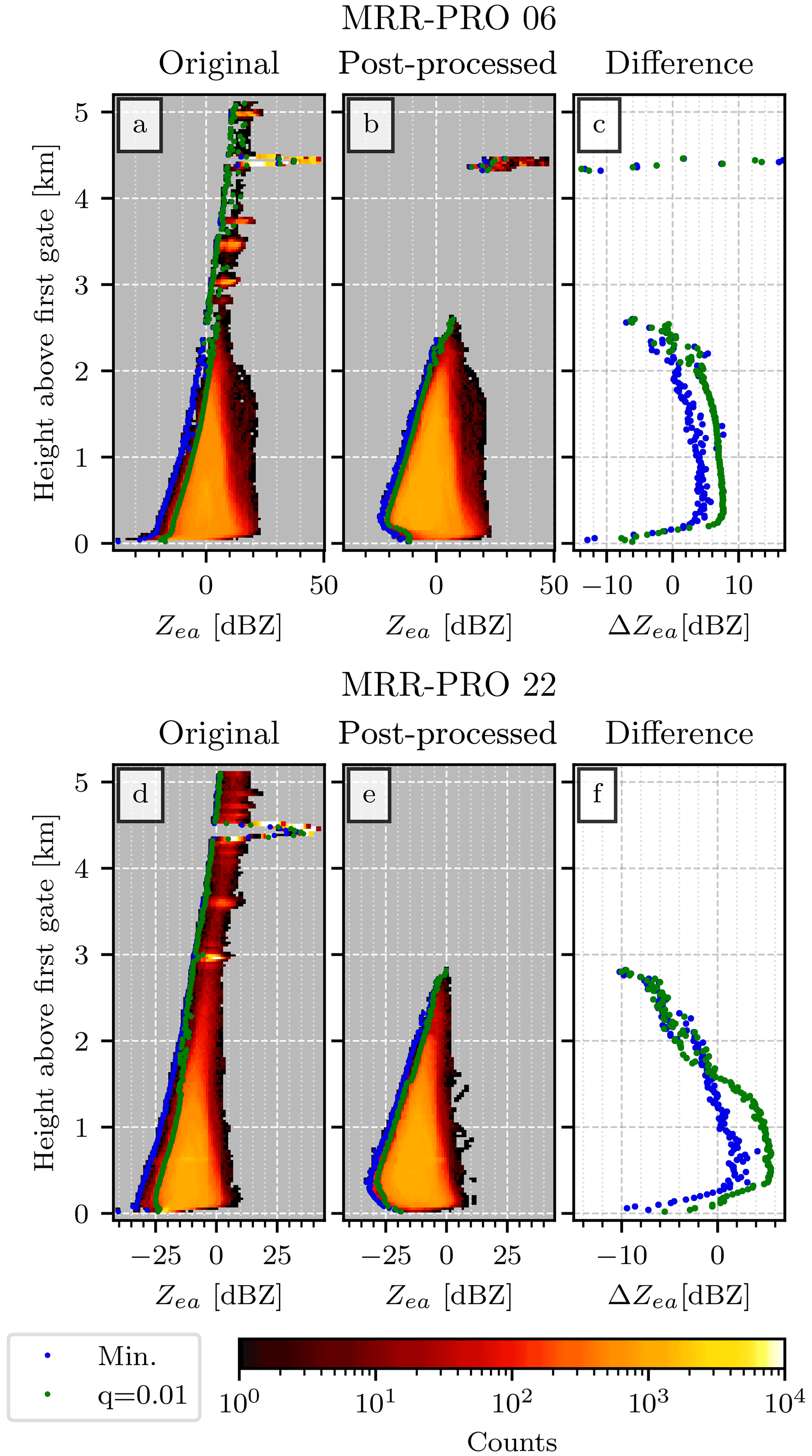
Figure 5Sensitivity curve for the MRR-PRO 06 (a, b, c) and MRR-PRO 22 (d, e, f) datasets. Panels (a) and (d) show a 2-dimensional histogram of the original attenuated equivalent reflectivity factor, while (b) and (e) display the post-processed one. The blue and green dots highlight the minimum and the quantile 0.01 of the Zea empirical distribution at each range gate, respectively. Note that the sensitivity of the MRR-PRO does not scale with range squared as a normal pulsed radar does. The differences between the two series of values (original MRR-PRO minus ERUO post-processed ones) are displayed in panels (c) and (f), following the same color convention as the previous panels.
The effects of interference lines on a dataset are visible in both Fig. 5a and d, where small, isolated clusters of bins with relatively high counts can be seen, starting from a height of around 3 km. A quick comparison with the examples shown in Fig. 1 confirms that the heights of the most important clusters are approximately the same as the strongest interference lines in Fig. 1a and c. In Fig. 5b, most of the effect of interferences is not visible anymore, except for the strongest one, at approximately 4.5 km. Additionally, the count associated with their bins is significantly lower than the one seen in Fig. 5a.
In Fig. 5d the interference clusters are accompanied by a large amount of noise, characterized by relatively low counts and reflectivity spanning a small interval close to the minimum detectable Zea. In the example shown in Fig. 1c, a few isolated signals can be seen above 4 km. They appear in almost every file, at random times and heights, and are often close to the minimum detectable reflectivity for their range gate. Given their random and faint appearance, we believe that they are just fluctuations in the raw spectrum that are incorrectly detected as signal, and we refer to them as “noise”. For the MRR-PRO 22 dataset, ERUO can produce a clean result by removing most of the noise, as can be seen in the upper part of Fig. 5e. The major interference line is also completely removed, contrary to what happened for the MRR-PRO 06 dataset.
In each of the mentioned four panels, two sets of dots are visible: the blue ones denote the minimum of the empirical distribution of Zea at each range gate, while the green ones show the quantile 0.01. Figure 5c and f display the difference between each set of statistics for the two campaigns, with a positive value indicating that the ERUO products reach a lower Zea at that specific range gate. We can observe two distinct behaviors for the two datasets.
For the MRR-PRO 06 we see an improvement for most of the lowest part of the profile, up to approximately 2 km above the first gate. Using the quantile 0.01 (green dots in Fig. 5c) as an estimate of the sensitivity, the improvement is between 4 and 8 dBZ, depending on the height. The minimum at each range gate (blue dots) gives us a smaller improvement, lower than 4 dBZ. However, it should be noted that in Fig. 5a the blue dots fall on a region of the histogram scarcely populated, and especially above 1 km, they are separated from the main cluster of counts. This behavior indicates, in our opinion, their belonging to the random noise that sometimes appears in the original measurements. While this noise appears more often in the MRR-PRO 22 dataset, it also exists in the MRR-PRO 06 one. This can be seen in Fig. 5a, where measurements are detected at each range gate above 3 km.
Above 2 km, the sensitivity difference in Fig. 5c rapidly turns negative, up to approximately 2.5 km, the maximum height at which precipitation has been detected in the dataset. Both the MRR-PRO 06 and the MRR-PRO 22 datasets have been collected at PEA, where precipitation events were relatively faint and shallow. The few isolated values above that height, visible in Fig. 5c, can be safely ignored since they refer to the interference lines visible in both products. For the MRR-PRO 22, in Fig. 5f, the sensitivity difference between the ERUO and original products is smaller. The estimate derived from the quantile 0.01 (green dots) is positive only until approximately 1.6 km, while the minimum one (blue dots) reaches 0 dBZ already at 1 km. We suspect that the drop in the difference in Fig. 5f is mostly caused by noise in the original files. While a small and sudden increase can be seen in the quantile 0.01 in Fig. 5e, at about 1.5 km of height, a larger change can be seen in Fig. 5d. As meteorological signal becomes more scarce with height, noise represents an increasingly higher fraction of the detected measurements. Therefore, the quantile 0.01 (green curve) becomes increasingly close to the minimum (blue curve), starting from approximately 1.5 km of height. This results in an artificial lowering of the estimated sensitivity of the original products. This interpretation is in agreement with the example of Fig. 1c and d. While ERUO provides a clearer image of the precipitation signal, the original products still contain a few low-reflectivity values at relatively high altitude. In particular, between 12:35 and 12:40 UTC we can see two measurements below −15 dBZ above 1 km, in clear contrast with the nearby precipitation signal. While such anomalous measurements also appear in the ERUO products, their impact on the 2-dimensional histogram of Fig. 5e is limited by the abundance of valid precipitation signals at the same height.
The same set of statistics computed over all datasets are displayed in Fig. 6, with the results for the ERUO processing output in the top row of panels and post-processing ones on the bottom row. The similarity between the couples of Fig. 6a and c and b and d indicates that the post-processing only has a marginal impact on the sensitivity gain.
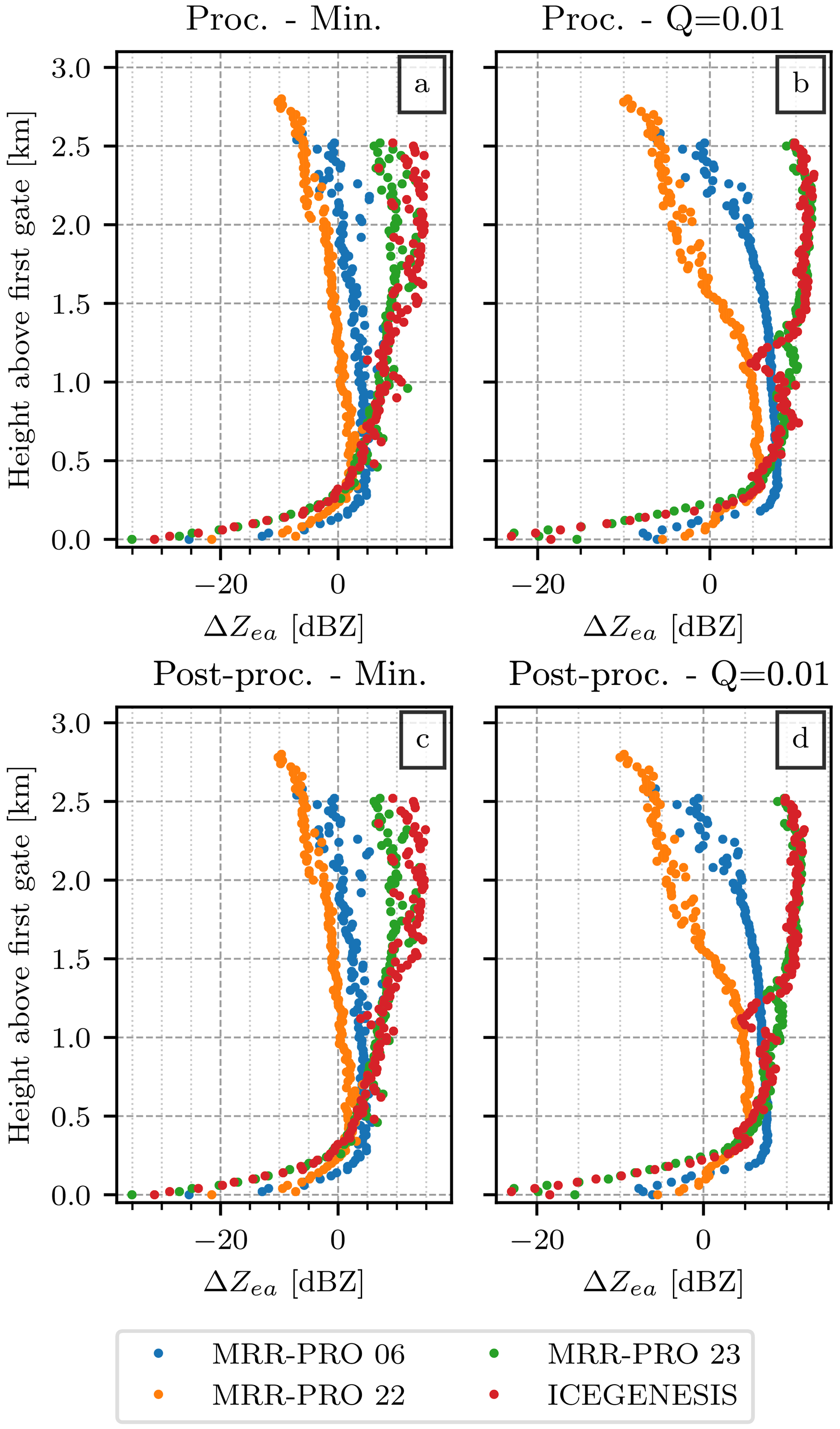
Figure 6Same as the panels (c) and (f) of Fig. 5, extended to the four datasets and including all products. Different colors are assigned to each dataset: blue for MRR-PRO 06, orange for MRR-PRO 22, green for MRR-PRO 23, and red for ICE GENESIS. Panels (a) and (b) display the difference for the ERUO processed products (original MRR-PRO minus ERUO), while panels (c) and (d) use the ERUO post-processed ones. For panels (a) and (c), the statistic used is the minimum value of the Zea empirical distribution at each range gate, while for panels (b) and (d) the statistic is the quantile 0.01. All figures have been truncated at 3.1 km since the only data points above that height are interference lines from the MRR-PRO 06.
The behavior of the red and green curve differs significantly from the other two. This is due to the transfer function issue, which radically affects the MRR-PRO 23 and ICE GENESIS measurements. As illustrated in Appendix B, the transfer function available in the original files of the two datasets has lower values than the correct one for most of the profile. This issue results in an artificial increase of Zea, which does not reflect the true intensity of the meteorological signal. Therefore, a direct comparison of its sensitivity with the other two MRR-PRO is not possible.
Finally, in the lowest range gates we always observe a lower minimum detectable reflectivity for the original products. Indeed, in the original files, Zea usually experiences a drop at low n. This can be seen in Fig. 1, especially in the comparisons of Fig. 1a with Fig. 1b or Fig. 1e with Fig. 1f. This drop may be caused by an incorrect noise floor estimation in the original algorithm by Metek, probably linked with the low raw spectra values typical of this region of the spectrum.
4.1.2 Direct comparison of radar variables
In this subsection we check how consistent the post-processed ERUO products are with the variables already available in the original MRR-PRO files.
As for the sensitivity estimate, we decided that the MRR-PRO 06 and MRR-PRO 22 datasets are the best choice for a fair comparison, given the absence of issues in the transfer function. Therefore, we decided to display the 2-dimensional histogram of the post-processed and original Zea of the two datasets in Fig. 7.

Figure 7Comparison between the Zea values available in the original MRR-PRO files (x axis) and the ones obtained at the end of the ERUO post-processing (y axis) for the MRR-PRO 22 dataset (a, b, c) and MRR-PRO 06 (d, e, f) datasets. The 1-dimensional histogram of the original Zea value is shown in panels (a) and (d), while the ERUO one is in panels (c) and (f). In panels (b) and (e), the blue line denotes the linear fit, while the green one shows the median difference between couples of measurements at the same (t,n).
Figure 7b offers the most direct comparison, given the better removal of interferences by ERUO for the MRR-PRO 22 dataset compared to the MRR-PRO 06 one. The central ridge of the histogram is relatively well aligned with the median difference (green line), which in turn is parallel to the identity line. A linear fit between the original and post-processed values also results in a line almost parallel to the identity line. At negative Zea, we observe a larger spread of the values. This behavior may be due to random noise appearing in the MRR-PRO 22 measurements at random heights close to the minimum detectable Zea, as discussed before. Since the sensitivity decreases with height, the noise affects a wide range of reflectivity values, between −30 and 0 dBZ.
The comparison for the MRR-PRO 06, shown in Fig. 7e, is instead plagued by the numerous interference lines visible in the upper right corner of the plot. Similarly to the MRR-PRO 22 case, the median difference (green line) is aligned with the central ridge of the histogram. The linear fit, however, deviates from it, probably due to the overabundance of clusters of measurements below the identity line at high Zea values. These clusters are likely caused by leftover interference lines, seen previously in Fig. 5b above 4 km. Finally, a large spread can be observed in the lowest reflectivity values, similarly to the MRR-PRO 22 case.
A similar comparison is repeated for the remaining two variables (V and SW). For completeness, we also included the other two datasets in the analysis, even though the issue with the transfer function necessarily results in enlarged differences for Zea. To summarize the results, we decided to compute three statistics from each comparison, each shown in a different row of Fig. 8: the median difference (original MRR-PRO products minus the ERUO ones) in Fig. 8a, b, and c, the interquartile range in Fig. 8d, e, and f, and the Pearson correlation coefficient in Fig. 8g, h, and i.
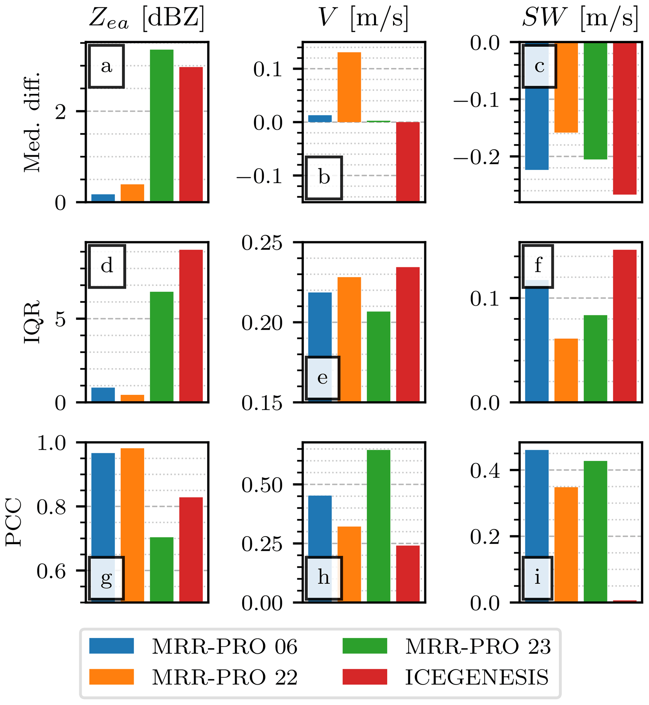
Figure 8Comparison of the ERUO post-processed products with the variables available in the original MRR-PRO files. The first row of panels (a, b, c) displays the median of the difference between corresponding entries in the two datasets (i.e., original minus ERUO). The second row (d, e, f) shows the interquartile range of the same difference. The third row (g, h, i) displays the Pearson correlation coefficient. Each column is associated with a different variable, indicated in the title at the top, together with its unit of measurement. Colors are assigned to each dataset following the same convention as Fig. 6. In panel (b), the fourth bar (ICE GENESIS dataset) reaches the value −18.1 m s−1.
From Fig. 8a we can estimate an offset between the ERUO and the original MRR-PRO products: lower than 0.5 dBZ in normal conditions and up to approximately 3.5 dBZ in presence of the issue with the transfer function. A part of the offset may be explained by the difference in the noise floor detection between ERUO and the algorithm used by Metek. We suspect that leftover interference lines may also be a contributor to this difference due to their consistently lower reflectivity values after the ERUO processing and post-processing, as shown by the sensitivity plots.
Among the Doppler velocity offset, the only noteworthy one is the ICE GENESIS one, close to −18 m s−1. The original MRR-PRO algorithm had problems in computing the variable, as confirmed in the next subsection, where the comparison with WProf is presented. The behavior may be similar to a problem with the Doppler velocity field described in Garcia-Benadi et al. (2020) for the MRR-2. Note that the Doppler velocity computation is unaffected by the transfer function issue, which results in a better agreement for the MRR-PRO 23 dataset.
More significant differences can be seen for the spectral width, in Fig. 8c. We suspect that it may be due to differences in signal detection. The higher sensitivity of ERUO may result in a lower noise level. Consequently, the peak associated with the detected signal may appear wider, resulting in a larger SW.
Figure 8d can be explained similarly to Fig. 8a, with the interference lines and noise playing a significant role in widening the spread of points around the identity line of the relative scatterplots. Figure 8e, instead, may be misleading. While the interquartile range (IQR) of the differences seems small, particularly large values can be found at the extremes of the empirical distribution of the differences. Due to the absence of an explicit antialiasing in the algorithm used by Metek for producing the original MRR-PRO products, several of the original V values are approximately vny apart from their ERUO counterpart.
The values of Pearson correlation coefficient in Fig. 8 are above 0.9 for the MRR-PRO 06 and MRR-PRO 22, as expected from the high level of agreement shown in Fig. 7. The transfer function differences negatively impact the correlation, especially for the MRR-PRO 23. While antialiasing may not affect directly the quantiles 0.25 and 0.75 used for Fig. 8e, its influence can be seen clearly in Fig. 8h. The correlation coefficient is significantly lower than in Fig. 8g for all datasets. While the ICE GENESIS case may be mostly explained by the −18.1 m s−1 shift in the original MRR-PRO values, the other datasets are still heavily affected by the aliasing, which aligns the V couples in an hypothetical scatterplot on three separate lines, parallel to the identity line.
4.2 Comparison with WProf
Given the presence of WProf alongside the MRR-PRO during the ICE GENESIS field campaign, we have access to an independent dataset for the verification of the ERUO products. Unfortunately, the MRR-PRO deployed at the site was affected by the issue in the transfer function, described in Appendix B. Any improvement in the agreement with WProf will be caused in large part by ERUO using the correct transfer function provided by Metek. Therefore, this section is not intended as an estimate of the improvements of the ERUO products compared to the original MRR-PRO variables but as an independent verification of the validity of the signal recovered by the proposed method.
Since the two radars record data at a different temporal and vertical resolution, we decided to remap the measures of WProf on the MRR-PRO resolutions, which are the coarsest. An example of the remapped data, alongside the two sets of MRR-PRO measurements, can be seen in Fig. 9. In Fig. 9c we can immediately spot the interference line typical of the ICE GENESIS dataset, just above the 1 km height mark. The line is almost completely eliminated by ERUO, and we can only see few traces of it in the precipitation signal in Fig. 9b. The difference of sensitivity between the two panels is also evident, especially at higher altitude. A third issue affects the profiles of Fig. 9c: Zea increases with height much faster than the WProf measurements of Fig. 9a. This behavior is particularly evident after 15:45 UTC, when the MRR-PRO measures an increase of reflectivity with height above 1.5 km, while WProf sees a decrease. This is caused by the transfer function issue mentioned before and discussed in Appendix B.
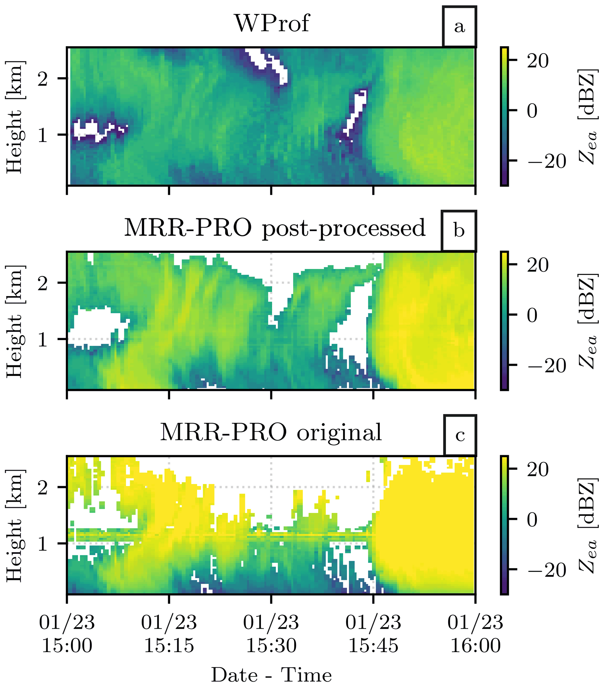
Figure 9Time series of attenuated equivalent reflectivity recorded by WProf (a) and the MRR-PRO (original Metek products in panel b, ERUO post-processing ones in panel c), covering 1 h of snowfall during the event on 23 January 2021.
Before extending the comparison of Zea to the whole ICE GENESIS campaign, we need to define clearly what measurements are suitable for it. Given the difference in frequency, we can expect that measurements in rainfall would be particularly attenuated for WProf. Therefore we decided to manually exclude the only rain event recorded in the period considered from the comparison. Additionally, large hydrometeors can be problematic since we could encounter cases in which the measurements at W-band are dominated by non-Rayleigh scattering, while the Rayleigh scattering is still valid at K-band. This occurrence would artificially increase the difference between the Zea measured at the two bands, spoiling the comparison. Thanks to the presence of MXPol at a few kilometers of distance from the site, we could use the results from both the hydrometeor classification (Besic et al., 2016) and the demixing algorithm (Besic et al., 2018) to extract profiles directly above the MRR-PRO and WProf site, giving us information on both the dominant hydrometeor type and the proportion of each hydrometeor class. After remapping them on the same MRR-PRO temporal and spatial resolutions mentioned before, we decided to use this information to select which radar volumes are suitable for the comparison. The first rule we defined is the most relaxed one: only volumes dominated by crystals, according to the classification results of Besic et al. (2016), will be used for the comparison between the MRR-PRO and WProf. Crystals are among the most common hydrometeor type in our dataset, and they are the smallest in size and therefore the most unlikely to cause an increase in the difference between the two bands. Naturally, we can expect some crystals to be particularly large and still become non-Rayleigh scatterers at W-band, but this would still be less common than for other hydrometeor classes with larger diameters. A second comparison is then performed on a stricter set of rules: in addition to enforcing a majority of crystals in the volumes, we also required that less than 20 % of the hydrometeors in it are aggregates, using the percentages provided by Besic et al. (2018). Aggregates are also common in our measurements, and they can reach sizes considerably bigger than crystals. As can be seen in Kneifel et al. (2015), the difference between the logarithmic difference of reflectivity values between X-band and W-band deviates the most from linearity when considering aggregates. This deviation is caused by aggregates becoming non-Rayleigh scatterers at W-band, a fact that would hold true also in our comparison, even though our comparison involves K-band instead of X-band.
Two 2-dimensional histograms obtained using this second set of rules are shown in Fig. 10. is compared with Zea(t,n) (Fig. 10b) and with the ERUO post-processed products (Fig. 10d). By comparing the two, we can immediately spot the effect of interference, causing a cluster in the top left corner of Fig. 10b, less marked in Fig. 10e. The most striking feature is the angle between the central ridge of higher counts in the 2-dimensional histogram and the median difference (green) line, visible in Fig. 10b. This behavior is obviously the effect of the transfer function issue. For Fig. 10e, instead, it appears that the central peak in the 2-dimensional histogram is approximately aligned with the green curve, parallel to the identity line. However, the spread remains large, with few outliers at low reflectivity values, probably caused by noise. We also suspect that the stronger attenuation at W-band compared to K-band may contribute to the relative abundance of measurements below the identity line.
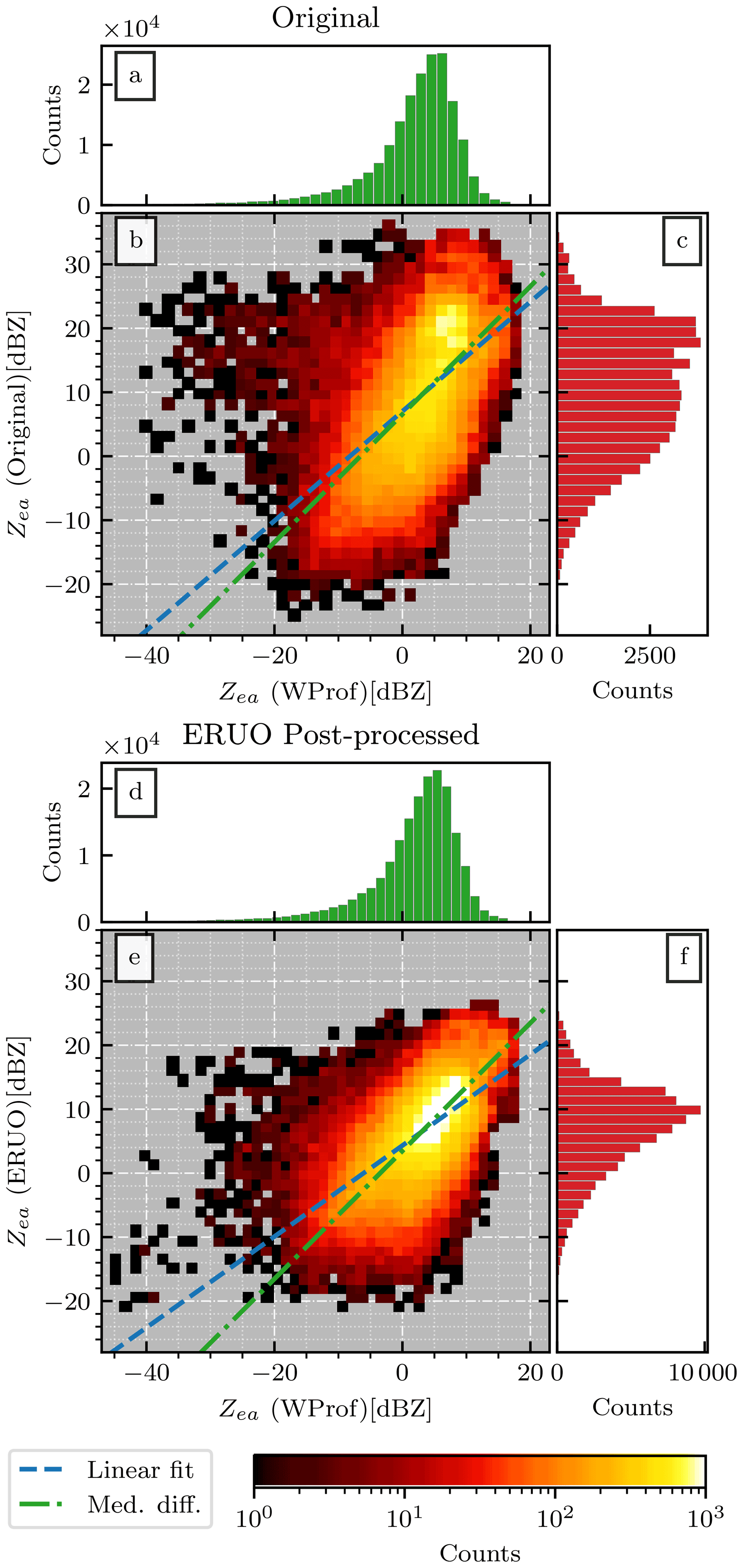
Figure 10Comparison between the Zea values recorded by WProf (x axis) and the MRR-PRO (y axis) during the ICE GENESIS campaign. The MRR-PRO reflectivity values in panels (a), (b), and (c) are computed by the original algorithm by Metek, while the ones in panels (d), (e), and (f) are the output of the ERUO post-processing. The 1-dimensional distribution for WProf, the original MRR-PRO attenuated reflectivity factor, and the one derived by ERUO are displayed in panels (a) (and panel d), (c), and (f) respectively. The green and blue lines in panels (b) and (e) follow the same convention as Fig. 7.
Similarly to the comparison presented in the previous subsection, we decided to summarize the results of the comparison for each variable in Fig. 11. ERUO appears to perform better than the original products in all panels. However, as explained at the beginning of this subsection, a significant part of the improvement for Zea can be attributed to the usage of the correct transfer function for the ERUO products. Additionally, in the case of Fig. 11a, the exact value of the median difference loses importance when we are unsure of the contribution of calibration differences on this offset. However, the improvements in interquartile range and correlation can, at least partially, be explained by the reduction of the contribution of interference lines. Intuitively, the latter appears in the 2-dimensional histogram as a cluster of high Zea for the MRR-PRO and low Zea for WProf, which enlarges the spread and worsens the overall correlation.
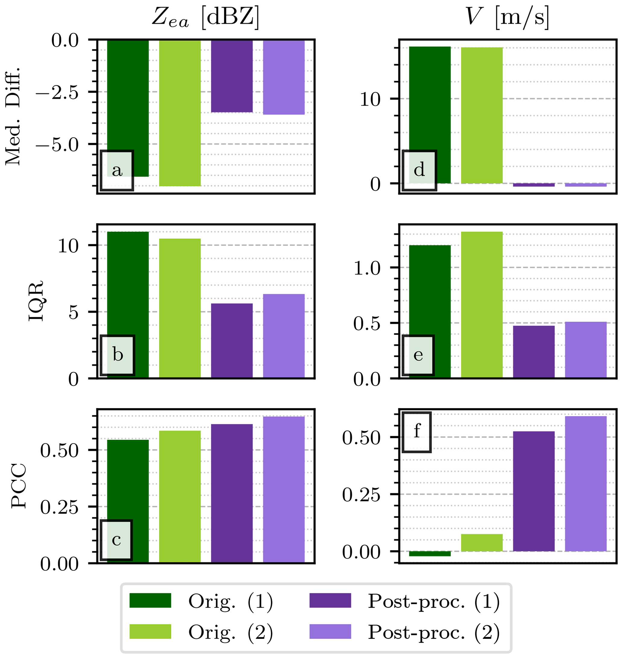
Figure 11Comparison between the ERUO post-processed products (Post-proc.), the variables available in the original MRR-PRO files (Orig.), and the ones recorded by WProf during the ICE GENESIS campaign. The figure follows the same layout as Fig. 8, with the exception of the SW column, which has not been included in the comparison. The numbers (1) and (2) appended to the name of the columns in the legend refers to which radar volumes have been included in the comparison. While (1) refers to the more relaxed condition involving only the dominant hydrometeor type, (2) also includes the threshold (20 %) on the proportion of aggregates present in the volume.
On the contrary, differences in Doppler velocity cannot be linked as directly to the transfer function since the variable depends mostly on the position of the recorded signal in the velocity range. Figure 11d shows that the ERUO products have a significantly smaller median difference from VW(t,n). This outcome is obviously linked with the issue with the Doppler velocity in the original MRR-PRO files previously mentioned. We observe a decrease of the interquartile range of the difference with WProf also for V, probably caused by the antialiasing.
Overall, even though a direct comparison of the original and ERUO products for this dataset is not completely fair, the improvement in the series of statistics displayed in Fig. 11 still confirms that ERUO is recovering valid measurements. As hinted by Fig. 9, many measurements that were below the sensitivity in the original products are now present in the ERUO ones. The improved agreement with WProf suggests that those newly visible signals are indeed valid precipitation measurements. They bring valid information, previously unavailable, to the dataset.
4.3 Performance of the spectrum reconstruction
The spectrum reconstruction plays a crucial role in creating a clean output, eliminating the strongest interferences before they can affect any of the variables. In all four datasets, interferences appear as spurious peaks in raw spectrum anomaly (A(i,n)). These peaks cover any return of lower intensity and they are masked by stronger signals. Since we cannot know what the real meteorological spectrum would have looked like without the interference, we cannot directly test the performance of our reconstruction.
However, we can extract some of these spurious peaks in A(i,n) and apply them to unaffected regions of the spectra from our datasets. Then, we can apply the spectrum reconstruction to these modified spectra, process them with ERUO, and compare outputs with the respective unaffected ones. If we process the modified spectra without first reconstructing them, we can also obtain a baseline that allows us to estimate the improvement brought by the reconstruction.
As a starting point, we extracted 180 examples of raw spectrum anomalies associated with interference lines, divided equally among the four datasets. We used IM(i,n) to define the extent of each anomaly. Four of them can be seen in Fig. 12, in which each panel shows the typical shape of the spurious peaks in A(i,n) for its respective dataset. Their exact position changes during the campaign, so the region extracted is usually larger than the main anomaly peak. These four interference types have been chosen to represent closely the variety that we observed. Therefore, even though the MRR-PRO used for the ICE GENESIS campaigns is the same MRR-PRO 23 deployed at PEA, different interference lines have been chosen to represent the two datasets. Additionally, since the anomaly in Fig. 12a is not symmetrical with respect to the vertical axis, we flipped half of them. Consequently, in the flipped anomalies, the rightmost peak becomes closer to lower velocity values, more likely to contain precipitation.

Figure 12Anomalies associated with interference lines extracted from clear-sky data from the four datasets. The name of the dataset from which each panel has been derived is displayed in its title. The ones displayed are just four examples out of the 180 matrices used in the spectrum reconstruction verification.
Since the extracted interferences are stored in a grid, we had to identify a region of similar size in each dataset in which . The chosen central gates are n=32 for the MRR-PRO 6, n=73 for the MRR-PRO 22, and n=125 the MRR-PRO 23. This selection allows for five extra range gates on each side of the region to avoid being too close to already existing interference lines. In addition to the constraints imposed by IM(i,n), the central gates have been spaced out through the profile to monitor the effect of interference at different heights.
An example of how the extracted anomalies are applied to a spectrum and of the subsequent reconstruction is shown in Fig. 13. Since the reconstruction acts on anomalies (A(i,n)) and not directly on the raw spectrum, we decided to display the former in the example figure. In Fig. 13a we highlighted the region to which the interference will be applied by delimiting its border with two dashed lines. As expected, the meteorological signal in the region seems unaffected by any noticeable spurious peak. In Fig. 13b, one of the anomaly matrices extracted from the ICE GENESIS dataset has been applied to the profile. At each set of coordinates (i,n), the resulting value has been chosen as the maximum between the original A(i,n) and the extracted interference anomaly. As a result, it is possible to see both the meteorological signal and three interference lines of different intensities. The spectrum reconstruction takes the resulting matrix as input and masks only a fraction of the entries, as shown in Fig. 13c, following the rules detailed in Sect. 3.2.1. Finally, the reconstructed anomaly is shown in the last panel. This output undergoes the standard processing, from which we derive Zea, V, and SW. The whole operation has been repeated for 120 profiles, divided equally among the three datasets collected at PEA.

Figure 13Example of reconstruction of the raw spectrum, performed during the verification phase. Panel (a) shows an example of unaltered spectra collected by the MRR-PRO 06. Once the interference matrix has been applied, the modified spectra are displayed in panel (b). Panel (c) illustrates the identification by ERUO of the region of the spectrum that needs to be reconstructed. Finally, the reconstructed spectra are shown in panel (d). The vertical extent of all panels has been truncated at n=100. The horizontal dotted line delimits the region in which the interference line has been added.
The variables derived from the reconstructed and altered profiles are compared with the ones computed from the original, unaltered raw spectra. The results of the comparison are shown in Fig. 14. The criteria used for the comparison are the mean absolute error (MEA) in the first row of panels, the root mean square error (RMSE) in the second, and the Pearson correlation coefficient (PCC) in the third. All comparison criteria are computed only over the range gates covered by newly added anomalies. Since the reconstruction often only affects a small fraction of these gates, the median difference could not be used to estimate the offset (or error, in this case) as done in the previous subsections, given its value that is almost always null.
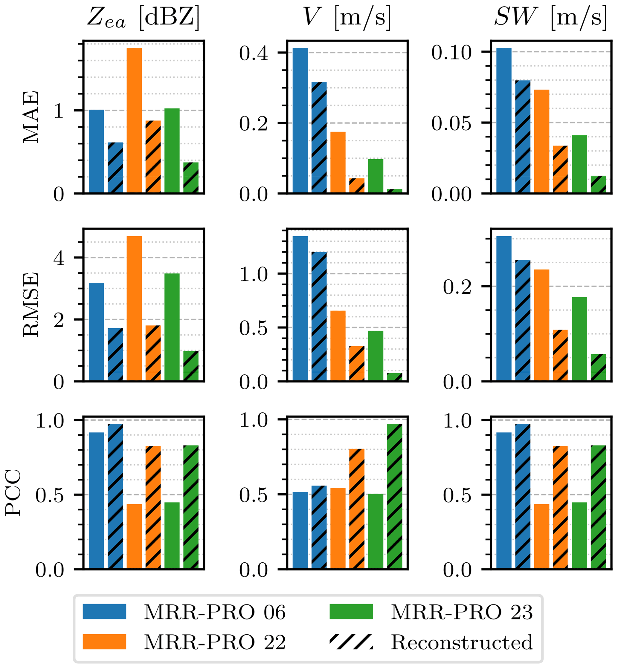
Figure 14Comparison of the variables computed starting from the modified spectra (plain columns) and the reconstructed one (black diagonal hatching) with the ones derived from the original, unaltered spectra. Colors are assigned to each dataset following the same convention as Fig. 6. The figure follows a similar layout to Fig. 8, with different scores: the mean absolute error (MEA) is displayed in the first row, while the root mean square error (RMSE) is shown in the second one.
The three statistics change significantly between the three MRR-PRO systems. This may be caused by the different characteristics of the precipitation signals at the three central heights at which the anomalies have been applied. The typical width and gradient of the signal vary with height, with the thinner and straighter spectra observed at higher altitudes being easier to reconstruct. To compute each of the three statistics, we need that a signal is detected, at least for a fraction of the range gates considered, in all three profiles: the reconstructed one, the modified one, and the unaltered one. Therefore, the comparison shown in the plot only takes into account precipitation data. Clear-sky measurements are not used for the computation of any of the statistics shown in Fig. 14.
The overlapping of meteorological signal and interference is the most complex situation to reconstruct for ERUO; therefore the skills discussed here represent a worst-case scenario. As exemplified by Fig. 9, the traces of the original interference line in the ERUO products can often only be seen over precipitation measurements and not in the clear-sky sections.
For all three datasets, the reconstruction reduces the error on the radar variables, while improving their correlation with the ones derived from the unaltered profiles. However, both MAE and RMSE indicate that the variables differ significantly from their ideal value. By observing a few examples of reconstruction, we could identify two critical situations that are not handled correctly by ERUO. The first one is the overlapping of precipitation signal with interference in the shape shown in Fig. 12a. As described in Sect. 3.2.1, the algorithm checks whether the interference is an isolated peak or a line spanning the whole range . When one of the two peaks shown in Fig. 12a intersects the precipitation signal, it falls in neither of the two categories, and it is not reconstructed. The second case is caused by weak interference, such as the one in Fig. 12b. Sometimes the anomaly is below the threshold used for masking it and therefore is never flagged for reconstruction. While this behavior could hypothetically be avoided by using a lower threshold, the latter may lead to an increase in false positives when flagging the pixels to reconstruct.
In this study we presented the ERUO library, a new processing technique for the MRR-PRO raw spectra, developed specifically for measurements in snowfall. The method has the twofold objective of minimizing the effect of a series of issues affecting the raw spectra, such as interference lines, and improving the quality of the output radar variables. The algorithm is divided into three stages, each with its own set of configurable parameters.
The first step, the preprocessing, uses information accumulated over an extended period of time to extract some quantities used in the correction of the raw spectra. In particular, the border correction BC(i,n), which compensates for the power drop at the extremes of the Doppler velocity range, is computed at this stage. Previous scientific work used interpolation to solve an analogous issue with the MRR-2 spectra, but this could lead to underestimation of the signal in the case of aliasing (Maahn and Kollias, 2012). However, the preprocessing introduces the first major limitation of the method: loading a large dataset at once may be problematic in some cases.
The next step, the processing, computes a series of variables using the preprocessing outputs and the raw spectra as a starting point. A crucial point during this procedure is the spectrum reconstruction. The interference mask (IM(i,n)) computed during the previous stage indicates region of the spectra likely to contain interference. A series of conditions aims to isolate only the location of the interference peak, and the meteorological signal that has been covered by it is estimated from the surrounding unaffected spectra. In the verification stage, particular attention has been dedicated to this reconstruction. We tested its performances by applying real interference anomalies from all our datasets to unaffected regions of the spectra collected by three MRR-PRO. The reconstruction results in variables closer to the ones obtained from the unaltered spectra, when compared to their non-reconstructed counterparts. A visual inspection of the MRR-PRO 06 reconstructed products shows that the reconstruction fails when isolated peaks, like the ones shown in Fig. 12a, partially overlap with meteorological signal. This behavior represents one of the most significant limitations of the proposed method. A possible future solution may involve the modification of the spectrum reconstruction routine by changing the conditions for interference in the form of isolated peaks.
The final products of the processing are the following variables: equivalent attenuated reflectivity factor (Zea), mean Doppler velocity (V), spectral width (SW), and signal-to-noise ratio (SNR). Concerning Zea, improvements between 4 and 8 dBZ can be seen in the sensitivity when compared to the original products. The improvement seems to taper off between 1.5 and 2.0 km above the first range gate. This occurrence may be caused by the low number of precipitation measurements above those heights in our datasets. The processing also involves a simple antialiasing based on the vertical continuity of the line connecting the local maxima of the spectrum at each range gate.
The last step of the algorithm is post-processing, which eliminates leftover interference lines and some isolated noise. Both processing and post-processing outputs are first compared with the original MRR-PRO variables over the four datasets. Due to a transfer function issue in the MRR-PRO 23 and ICE GENESIS datasets, a direct comparison of Zea is only meaningful for the MRR-PRO 06 and MRR-PRO 22. For the Zea in these two datasets we observe the best agreement, with a median difference always within 0.5 dBZ and a Pearson correlation coefficient above 0.9. The agreement is lower for V and SW, which are more affected by the lack of antialiasing in the original MRR-PRO processing algorithm.
A comparison of the Zea and V measurements with a second radar, WProf, has also been performed. Only the ICE GENESIS dataset has been used in this case since it is the only one in which the two radars were co-located. Unfortunately, MRR-PRO 23 was used for this campaign, and its measurements are affected by the transfer function issue. The analysis has been repeated for two different sets of conditions, first imposing a prerequisite on the sole dominant hydrometeor type (ice crystals) and then also on the maximum proportion of aggregates (20 %). In both cases, the ERUO processing results in a lower median and IQR of the difference between the two radars and a higher Pearson correlation coefficient. Unfortunately, the original products are affected by an issue in the transfer function and the velocity computation. Therefore, the results of the comparison can be used as independent verification of the validity of the ERUO products but not as a fair comparison between the latter and the original MRR-PRO variables. Overall, the agreement between the ERUO variables and the ones collected by WProf suggests that the former is recovering valid measurements.
Finally, an achievement of the ERUO processing that may be hard to quantify is the enhancement in the readability of the precipitation structure in time–height plots. ERUO can recover meteorological signals that were too faint to be recorded in the variables computed by the Metek algorithm in the original data files, especially at higher altitudes. As can be seen in Figs. 1 and 9, the removal of the main interference line and the improvement in sensitivity result in a much clearer series of profiles, in which the structure of the precipitation system can be more easily be understood.
This section details the steps involved in the creation of the three preprocessing products introduced in Sect. 3.1.
A1 First iteration
The main aim of this first step of the preprocessing is the removal of isolated and anomalous spectral density peaks in . Their presence can seriously impact Pe(n) by artificially raising the estimated clear-sky power level at the range gates affected by these spikes. Key steps of the first iterations are exemplified, for the MRR-PRO 06, in Fig. A1, with as the starting point in Fig. A1a.
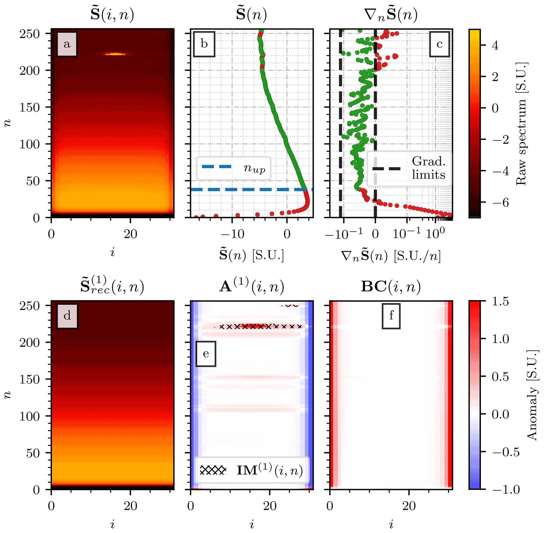
Figure A1The first iteration of the preprocessing of the MRR-PRO 06 dataset. Panel (a) shows . Panel (b) displays its median value at each range gate () with the entries used in the fit of the median profile colored in green and the excluded ones in red, with the dashed blue line at n=nup delimiting the upper region. Panel (c) shows the vertical gradient of , with the same color coding as panel (b). The vertical dashed black lines denote the limits for accepted gradient values. The reconstructed median profile obtained by tiling m times is shown in panel (d). Panel (e) shows the anomaly from this baseline profile (A(1)(i,n)), with the superimposed hatching representing the first estimated interference mask (IM(1)(i,n)). Finally, panel (f) displays the first product of the preprocessing, BC(i,n).
To identify these spurious signals, we first need to define a rough estimate of the background power level at each range gate. Therefore, a quantity akin to an early guess of Pe(n) is defined following this procedure:
-
The median of at each range gate, denoted by , is computed. Its vertical gradient, , is also estimated. Examples of both quantities for the MRR-PRO 06 dataset are shown in Fig. A1c.
-
Given the observed trend of the median spectrum, we decided to treat separately the lowest part of the profile (power increasing with height) and the second one (inverse trend). This step is necessary for accurately identifying peaks in the spectrum, which is possible with our method only in the upper part of the profile. The first step is the identification of the range gate in which changes in sign, which provides a first guess of the beginning of the upper section of the profile. This estimate is refined by excluding a few range gates at the beginning of the section, where is closer to zero, and the raw spectrum plateaus. More precisely, the beginning of this second part of the profile is moved to the first n in which reaches the median value of all negative . We will refer to this range gate as nup. Figure A1b shows the location of nup for the MRR-PRO 06, while Fig. A1c displays how, immediately after the change of sign, the gradient does not reach the negative value typical of the upper part of the profile.
-
We now focus on the upper part of , for n>nup. This is the region most often affected by interference lines, which may lead to spurious peaks in the Pe(n) estimate. To exclude them, the algorithm imposes two thresholds on . The maximum is set to 0 since the overall trend of the power profile in this region is towards lower values, and a positive derivative can only indicate the presence of a peak. The lower one instead aims to exclude the descending part of the spurious peak. The exact threshold value is set equal to the median for n>nup multiplied by a constant. This constant is set by default to 3. From a visual inspection of the final preprocessing products, this value highlights the major peaks without masking all the fainter lines, which may create problems in the reconstruction. The distinction between faint and strong interference lines is arbitrary. Therefore we cannot judge exactly what proportion of each category is included or excluded. This specific value resulted in the masking of all the interference lines that we considered major in the four datasets while masking only a few (approximately five, depending on the dataset) minor lines. However, as for all the parameters of ERUO, its value can be changed in the configuration file.
-
We compute a smoother version of this upper part of the profile, by performing a polynomial fit of , for n>nup and excluding the range gates that do not satisfy the thresholds described above. After some tests, the degree of the polynomial has been set to 4. While it appears that the fit is not very sensitive to small changes, such as increasing or lowering the degree by one, the chosen value seems to provide a curve that better maintains the profile trend, even if we were to extend the range to . This may reduce the risk of contaminating the final part of the profile with the effect of a spurious inversion of the trend a few gates after the end of the fitted range. We will refer to the fit result as .
-
Finally, we can define our early guess for the power received in each range gate in ideal clear-sky conditions. Since the curve presented here is just a first estimate, we use the symbol for it. For n≤nup, we set equal to . For the upper part, instead, we set equal to the element-wise minimum between and , to avoid the risk of artificially increasing the baseline power level.
A 2-dimensional matrix, , is created by tiling m times the newly computed across a new dimension. This newly defined quantity represents a reconstruction of with a lowered impact of the interference lines since the strongest peaks are excluded from the input of the polynomial fit. This matrix, computed for the MRR-PRO 06, is shown in Fig. A1d. Even though it is only a preliminary estimate of the clear-sky raw spectrum, the reduced impact of interference and the lack of a drop at both ends of the Doppler velocity range can immediately be spotted.
Both features are enhanced when looking at the anomaly from this baseline raw spectrum, defined as . This matrix is used to compute IM(1)(i,n), a partial interference mask, covering only the isolated anomalous spikes in the spectrum. Both A(1)(i,n) and IM(1)(i,n) (for MRR-PRO 06) can be seen in Fig. A1e.
The computation of IM(1)(i,n) starts by masking (i.e., setting equal to 1) all regions where S.U. Once again, this assumption is only valid if does not contain any leftover precipitation signal. Then, the columns i=1, 2, 3, m−2, m−1, and m are all unmasked (i.e., set equal to 0) since the power drop at those spectral lines has not been corrected yet. Finally, all range gates containing at least m−6 masked values are also artificially removed from the mask, since IM(1)(i,n) aims to cover only the isolated peaks and not the ones spanning the whole range . Notice how in Fig. A1e some interference lines (especially the fainter ones) extend throughout the whole Doppler velocity range, while IM(1)(i,n) only targets the central part of the spectrum.
The threshold 0.2 is the lowest one that allowed for the masking of all the most visible interference in our four datasets. The decision of excluding the three last spectral line numbers on the two extremes of the velocity range is motivated by the drop in raw spectrum, more marked in those columns for all our datasets.
The border correction BC(i,n), the first product of the preprocessing, is introduced to correct for this drop. After masking all regions of where , the median of the remaining valid values at each range gate is computed and tiled m times, resulting in a 2-dimensional matrix, . This matrix is usually similar to the one displayed in Fig. A1d. However, while the latter is based on our reconstruction, is entirely based on a subset of the measured data. Then, BC(i,n) is defined as equal to for the couples (i,n) for which and 0 everywhere else. Figure A1f shows the result for the MRR-PRO 06.
A2 Second iteration
The main product of the first iteration, BC(i,n), allows us to refine most of the previous estimates by reducing the impact of the power drop for i close to 1 or m. Without this first estimate of the border correction, it would have been impossible to accurately define an interference mask. The typical power drop at the extreme i can be lower than 1 , while the faintest of the interference lines can be constituted by anomalies as low as 0.2 , by definition. Therefore, the first can hide the second in some regions of the spectrum. This outcome would result in the final products of the processing retaining these unmasked sections of the interference lines, defying the whole purpose of the preprocessing.
As the starting point of this second iteration of the preprocessing, we define a new quantity: . Using it in place of , we repeat steps 1–5 of Sect. A1. The resulting reconstructed profile is Pe(n), one of the final products of the preprocessing.
As in the previous subsection, a 2-dimensional matrix is derived by repeating m times Pe(n) across a new dimension. This matrix is subtracted from , giving us the new anomaly, A(2)(i,n). To compute IM(i,n), the algorithm starts by masking (setting equal to 1) all entries (i,n) where S.U. If at a specific range gate number more than 0.9×m are masked, all the remaining values at that n will be masked, too. Finally, the mask undergoes a series of three binary dilations. Each expands the mask to pixels adjacent to already masked ones (excluding the diagonal from the contiguity).
As mentioned when IM(i,n) was first introduced, the mask aims to cover the regions likely to contain interference. The latter appears in the spectrum as peaks or lines, whose exact position is changing during the campaign, and it may vary slightly in both i and n. While the median spectrum, at the base of this preprocessing, captures the most likely position for the various peaks and lines, variations in their locations may appear too seldom to leave a trace strong enough to be detected as interference. This is why the binary dilation and the threshold on the maximum number of masked spectral lines at any range gate have been introduced: they artificially expand the mask, resulting in a more likely coverage of these rare variations. The exact values for the parameters controlling the two operations have been set after a series of trials on our datasets. The final choice was a compromise: while the spectrum reconstruction (Sect. 3.2.1) improves for smaller masked regions, the contamination by interference in the final output of ERUO is reduced when the mask is expanded.
The transfer function is used by FMCW radars to include the receiver gain dependence on the range gate number in the conversion of the raw spectra into spectral reflectivity. As visible in Fig. B1a, the codomain of a normal transfer function (in black) is approximately confined between 0 and 1.
In the ICE GENESIS and MRR-PRO 23 datasets, collected by the same MRR-PRO, this function appears to have a sudden jump at n=128 (approximately 2000 m above the radar in our configuration), with its value increasing by a factor of approximately 1038. The jump is displayed in Fig. B1a, represented by the almost vertical orange line connecting the last valid transfer function entry and the next, extremely high one. Therefore, the final radar variables available in the data file appear truncated at that range gate.
The issue was easily solved by contacting Metek. They provided us with the correct transfer function for the radar. The path to the file containing this transfer function can be provided to ERUO in the configuration file. A flag in the same file controls whether ERUO uses this external transfer function or the one available in the MRR-PRO files for the processing.
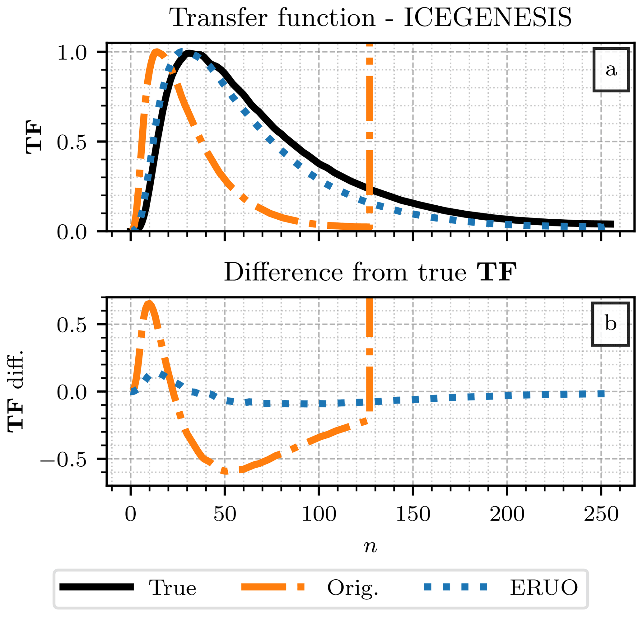
Figure B1Comparison of transfer functions for the ICE GENESIS dataset. Panel (a) shows three transfer functions: the true one (provided by Metek) in black, the corrupted one available in the original files in orange, and the one reconstructed by ERUO in blue. Panel (b) presents the differences: in blue the ERUO one minus the true one and in orange the original one minus the true one.
However, in case it is not possible to recover the correct transfer function, ERUO can try to estimate it from the truncated one available in the MRR-PRO file. This optional step in the processing routine is called transfer function reconstruction. It resamples TF(n) over the correct nmax.
The algorithm starts by checking for entries in TF(n) above a certain threshold, set by default to 9×10⁹, and masks them. Then, using the “scipy.signal.resample” function (Virtanen et al., 2020), the unmasked section of the function is resampled over a number of samples equal to nmax. The result is finally rescaled to ensure that the height of its maximum peak is the same as the unmasked section of the original function. In Fig. B1, the final output for the ICE GENESIS (and MRR-PRO 23) dataset is displayed as a dotted blue line.
As highlighted by the difference shown in Fig. B1b, the reconstruction is not perfect. If the true transfer function can be recovered, the reconstruction should be avoided. However, when recovering it is impossible; the difference between the reconstructed transfer function and the true one is smaller than the one computed starting from the corrupted transfer function available in the original files. The improvement is especially noticeable for n>30, where the reconstructed transfer function follows the true one more closely.
The following symbols are used in the main text of this paper.
| Power anomaly (difference between raw spectrum and clear-sky estimate) | |
| BC(i,n) | Border correction |
| c | Calibration constant |
| EXC(t,n) | Matrix of the measurements flagged for removal during the post-processing |
| Raw spectrum in linear units, after the spectrum reconstruction | |
| The signal extracted from , after the noise subtraction | |
| Spectral line number | |
| IM(i,n) | Interference mask |
| Range gate number | |
| NL(1)(t,n) | First estimate of the noise level |
| NL(t,n) | Final estimate of the noise level |
| Pe(n) | Signal-free raw spectrum profile estimate |
| Raw spectrum | |
| Raw spectrum corrected at the velocity extremes | |
| Clear-sky estimate of the power return, obtained tiling Pe(n) | |
| Median raw spectrum across all time steps | |
| SNR(t,n) | Signal-to-noise ratio (MRR-PRO, original files) |
| SNR(Proc)(t,n) | Signal-to-noise ratio (MRR-PRO, processing output) |
| SNRW(t,n) | Signal-to-noise ratio (WProf) |
| SW(t,n) | Spectral width (MRR-PRO, original files) |
| SW(Proc)(t,n) | Spectral width (MRR-PRO, processing output) |
| Attenuated equivalent spectral reflectivity factor in linear units | |
| t | Time |
| TF(n) | Transfer function |
| V(t,n) | Doppler radial velocity (MRR-PRO, original files) |
| V(Proc)(t,n) | Doppler radial velocity (MRR-PRO, processing output) |
| VW(t,n) | Doppler radial velocity (WProf) |
| Zea(t,n) | Attenuated equivalent reflectivity factor (MRR-PRO, original files) |
| Attenuated equivalent reflectivity factor (MRR-PRO, processing output) | |
| Attenuated equivalent reflectivity factor (WProf) |
The ERUO library is available for download at https://github.com/alfonso-ferrone/ERUO.git (last access: 8 June 2022; https://doi.org/10.5281/zenodo.6623344, Ferrone, 2022).
The datasets used in the paper have not been made available yet at the time of writing, since they will be published as part of two different papers in the near future. However, the data are available upon request from the contact author.
AF and AB designed the study, with inputs from ACBR on the verification section. AF and AB deployed and maintained the instruments at PEA. ACBR and AB deployed and maintained the instruments for ICE GENESIS. AF processed the data for PEA, and ACBR processed the ones for ICE GENESIS, including executing the hydrometeor classification and demixing algorithm for the MXPol data. AF prepared the manuscript with contributions from ACBR and AB and supervision from AB. All authors have read and agreed to the published version of the paper.
At least one of the (co-)authors is a member of the editorial board of Atmospheric Measurement Techniques. The peer-review process was guided by an independent editor, and the authors also have no other competing interests to declare.
Publisher’s note: Copernicus Publications remains neutral with regard to jurisdictional claims in published maps and institutional affiliations.
We would like to thank all the EPFL–LTE collaborators involved in the deployment and management of the radars during the field campaigns at PEA and ICE GENESIS. We are grateful to all the personnel of the PEA station, including management, technicians, field guides, and everyone at the station that made the campaign possible. We are also thankful to the personnel of the airport of La Chaux-de-Fonds for their assistance in various stages of the installation and removal of the instruments. Finally, we greatly appreciated the innumerable suggestions of Josué Gehring, Gionata Ghiggi, and Monika Feldmann, which aided us in shaping the algorithm and the subsequent verification.
This research has been supported by the Schweizerischer Nationalfonds zur Förderung der Wissenschaftlichen Forschung (grant no. 200020-175700/1) and the Swiss Polar Institute (Polar Access Fund 2019 and Exploratory Grant).
This paper was edited by Stefan Kneifel and reviewed by three anonymous referees.
Alexander, S.: Precipitation over Land and the Southern Ocean (PLATO) Field Campaign Report, Office of Scientific and Technical Information, U.S. Department of Energy, https://www.osti.gov/biblio/1524773 (last access: 8 June 2022), 2019. a
Astropy Collaboration, Robitaille, T. P., Tollerud, E. J., Greenfield, P., Droettboom, M., Bray, E., Aldcroft, T., Davis, M., Ginsburg, A., Price-Whelan, A. M., Kerzendorf, W. E., Conley, A., Crighton, N., Barbary, K., Muna, D., Ferguson, H., Grollier, F., Parikh, M. M., Nair, P. H., Unther, H. M., Deil, C., Woillez, J., Conseil, S., Kramer, R., Turner, J. E. H., Singer, L., Fox, R., Weaver, B. A., Zabalza, V., Edwards, Z. I., Azalee Bostroem, K., Burke, D. J., Casey, A. R., Crawford, S. M., Dencheva, N., Ely, J., Jenness, T., Labrie, K., Lim, P. L., Pierfederici, F., Pontzen, A., Ptak, A., Refsdal, B., Servillat, M., and Streicher, O.: Astropy: A community Python package for astronomy, Astron. Astrophys., 558, A33, https://doi.org/10.1051/0004-6361/201322068, 2013. a
Astropy Collaboration, Price-Whelan, A. M., Sipőcz, B. M., Günther, H. M., Lim, P. L., Crawford, S. M., Conseil, S., Shupe, D. L., Craig, M. W., Dencheva, N., Ginsburg, A., VanderPlas, J. T., Bradley, L. D., Pérez-Suárez, D., de Val-Borro, M., Aldcroft, T. L., Cruz, K. L., Robitaille, T. P., Tollerud, E. J., Ardelean, C., Babej, T., Bach, Y. P., Bachetti, M., Bakanov, A. V., Bamford, S. P., Barentsen, G., Barmby, P., Baumbach, A., Berry, K. L., Biscani, F., Boquien, M., Bostroem, K. A., Bouma, L. G., Brammer, G. B., Bray, E. M., Breytenbach, H., Buddelmeijer, H., Burke, D. J., Calderone, G., Cano Rodríguez, J. L., Cara, M., Cardoso, J. V. M., Cheedella, S., Copin, Y., Corrales, L., Crichton, D., D'Avella, D., Deil, C., Depagne, É., Dietrich, J. P., Donath, A., Droettboom, M., Earl, N., Erben, T., Fabbro, S., Ferreira, L. A., Finethy, T., Fox, R. T., Garrison, L. H., Gibbons, S. L. J., Goldstein, D. A., Gommers, R., Greco, J. P., Greenfield, P., Groener, A. M., Grollier, F., Hagen, A., Hirst, P., Homeier, D., Horton, A. J., Hosseinzadeh, G., Hu, L., Hunkeler, J. S., Ivezić, Ž., Jain, A., Jenness, T., Kanarek, G., Kendrew, S., Kern, N. S., Kerzendorf, W. E., Khvalko, A., King, J., Kirkby, D., Kulkarni, A. M., Kumar, A., Lee, A., Lenz, D., Littlefair, S. P., Ma, Z., Macleod, D. M., Mastropietro, M., McCully, C., Montagnac, S., Morris, B. M., Mueller, M., Mumford, S. J., Muna, D., Murphy, N. A., Nelson, S., Nguyen, G. H., Ninan, J. P., Nöthe, M., Ogaz, S., Oh, S., Parejko, J. K., Parley, N., Pascual, S., Patil, R., Patil, A. A., Plunkett, A. L., Prochaska, J. X., Rastogi, T., Reddy Janga, V., Sabater, J., Sakurikar, P., Seifert, M., Sherbert, L. E., Sherwood-Taylor, H., Shih, A. Y., Sick, J., Silbiger, M. T., Singanamalla, S., Singer, L. P., Sladen, P. H., Sooley, K. A., Sornarajah, S., Streicher, O., Teuben, P., Thomas, S. W., Tremblay, G. R., Turner, J. E. H., Terrón, V., van Kerkwijk, M. H., de la Vega, A., Watkins, L. L., Weaver, B. A., Whitmore, J. B., Woillez, J., Zabalza, V., and Astropy Contributors: The Astropy Project: Building an Open-science Project and Status of the v2.0 Core Package, Astron. J., 156, 123, https://doi.org/10.3847/1538-3881/aabc4f, 2018. a
Besic, N., Figueras i Ventura, J., Grazioli, J., Gabella, M., Germann, U., and Berne, A.: Hydrometeor classification through statistical clustering of polarimetric radar measurements: a semi-supervised approach, Atmos. Meas. Tech., 9, 4425–4445, https://doi.org/10.5194/amt-9-4425-2016, 2016. a, b, c
Besic, N., Gehring, J., Praz, C., Figueras i Ventura, J., Grazioli, J., Gabella, M., Germann, U., and Berne, A.: Unraveling hydrometeor mixtures in polarimetric radar measurements, Atmos. Meas. Tech., 11, 4847–4866, https://doi.org/10.5194/amt-11-4847-2018, 2018. a, b, c
Ferrone, A.: alfonso-ferrone/ERUO: v1.0.1-ERUO (v1.0.1), Zenodo [code], https://doi.org/10.5281/zenodo.6623344, 2022. a
Foth, A., Zimmer, J., Lauermann, F., and Kalesse-Los, H.: Evaluation of micro rain radar-based precipitation classification algorithms to discriminate between stratiform and convective precipitation, Atmos. Meas. Tech., 14, 4565–4574, https://doi.org/10.5194/amt-14-4565-2021, 2021. a
Garcia-Benadi, A., Bech, J., Gonzalez, S., Udina, M., Codina, B., and Georgis, J.-F.: Precipitation Type Classification of Micro Rain Radar Data Using an Improved Doppler Spectral Processing Methodology, Remote Sens., 12, 4113, https://doi.org/10.3390/rs12244113, 2020. a, b, c
Gorodetskaya, I. V., Kneifel, S., Maahn, M., Van Tricht, K., Thiery, W., Schween, J. H., Mangold, A., Crewell, S., and Van Lipzig, N. P. M.: Cloud and precipitation properties from ground-based remote-sensing instruments in East Antarctica, The Cryosphere, 9, 285–304, https://doi.org/10.5194/tc-9-285-2015, 2015. a
Grazioli, J., Genthon, C., Boudevillain, B., Duran-Alarcon, C., Del Guasta, M., Madeleine, J.-B., and Berne, A.: Measurements of precipitation in Dumont d'Urville, Adélie Land, East Antarctica, The Cryosphere, 11, 1797–1811, https://doi.org/10.5194/tc-11-1797-2017, 2017. a
Hildebrand, P. H. and Sekhon, R.: Objective determination of the noise level in Doppler spectra, J. Appl. Meteorol., 13, 808–811, https://doi.org/10.1175/1520-0450(1974)013<0808:ODOTNL>2.0.CO;2, 1974. a, b
ICE GENESIS Consortium: ICE GENESIS H2020 Project – Creating the next generation of 3D simulation means for icing, https://www.ice-genesis.eu/ (last access: 8 June 2022), 2021. a
Klugmann, D., Heinsohn, K., and Kirtzel, H. J.: A low cost 24 GHz FM-CW Doppler radar rain profiler, 3. international symposium on tropospheric profiling: needs and technologies, Hamburg, Germany, 30 August–2 September 1994, in: Contributions to atmospheric physics, vol. 69, Report Number: CONF-9408118, 1996. a
Kneifel, S., von Lerber, A., Tiira, J., Moisseev, D., Kollias, P., and Leinonen, J.: Observed relations between snowfall microphysics and triple-frequency radar measurements, J. Geophys. Res.-Atmos., 120, 6034–6055, https://doi.org/10.1002/2015JD023156, 2015. a
Küchler, N., Kneifel, S., Löhnert, U., Kollias, P., Czekala, H., and Rose, T.: A W-band radar–radiometer system for accurate and continuous monitoring of clouds and precipitation, J. Atmos. Ocean. Tech., 34, 2375–2392, 2017. a
Maahn, M. and Kollias, P.: Improved Micro Rain Radar snow measurements using Doppler spectra post-processing, Atmos. Meas. Tech., 5, 2661–2673, https://doi.org/10.5194/amt-5-2661-2012, 2012. a, b, c, d, e, f
Pishniak, D., Krakovska, S., Chyhareva, A., and Razumnyi, S.: Preliminary analysis and main problems of instrumental measurement complex at the Vernadsky Antarctic Station, EGU General Assembly 2021, online, 19–30 April 2021, EGU21-13591, https://doi.org/10.5194/egusphere-egu21-13591, 2021. a
Saltikoff, E., Friedrich, K., Soderholm, J., Lengfeld, K., Nelson, B., Becker, A., Hollmann, R., Urban, B., Heistermann, M., and Tassone, C.: An Overview of Using Weather Radar for Climatological Studies: Successes, Challenges, and Potential, B. Am. Meteorol. Soc., 100, 1739–1752, https://doi.org/10.1175/BAMS-D-18-0166.1, 2019. a
Schneebeli, M., Dawes, N., Lehning, M., and Berne, A.: High-resolution vertical profiles of X-band polarimetric radar observables during snowfall in the Swiss Alps, J. Appl. Meteorol. Clim., 52, 378–394, 2013. a
Segelstein, D. J.: The complex refractive index of water, PhD thesis, University of Missouri–Kansas City, http://hdl.handle.net/10355/11599 (last access: 14 June 2022), 1981. a
Virtanen, P., Gommers, R., Oliphant, T. E., Haberland, M., Reddy, T., Cournapeau, D., Burovski, E., Peterson, P., Weckesser, W., Bright, J., van der Walt, S. J., Brett, M., Wilson, J., Millman, K. J., Mayorov, N., Nelson, A. R. J., Jones, E., Kern, R., Larson, E., Carey, C. J., Polat, İ., Feng, Y., Moore, E. W., VanderPlas, J., Laxalde, D., Perktold, J., Cimrman, R., Henriksen, I., Quintero, E. A., Harris, C. R., Archibald, A. M., Ribeiro, A. H., Pedregosa, F., van Mulbregt, P., and SciPy 1.0 Contributors: SciPy 1.0: Fundamental Algorithms for Scientific Computing in Python, Nat. Methods, 17, 261–272, https://doi.org/10.1038/s41592-019-0686-2, 2020. a, b
- Abstract
- Introduction
- Data
- Method
- Validation
- Summary and conclusions
- Appendix A: Preprocessing
- Appendix B: Transfer function issues
- Appendix C: List of symbols
- Code availability
- Data availability
- Author contributions
- Competing interests
- Disclaimer
- Acknowledgements
- Financial support
- Review statement
- References