Cloud phase and macrophysical properties over the Southern Ocean during the MARCUS field campaign

To investigate the cloud phase and macrophysical properties over the Southern Ocean (SO), the Department of Energy (DOE) Atmospheric Radiation Measurement (ARM) Mobile Facility (AMF2) was installed on the Australian icebreaker research vessel (R/V) Aurora Australis during the Measurements of Aerosols, Radiation, and Clouds over the Southern Ocean (MARCUS) field campaign (41 to 69^∘ S, 60 to 160^∘ E) from October 2017 to March 2018. To examine cloud properties over the midlatitude and polar regions, the study domain is separated into the northern (NSO) and southern (SSO) parts of the SO, with a demarcation line of 60^∘ S. The total cloud fractions (CFs) were 77.9 %, 67.6 %, and 90.3 % for the entire domain, NSO and SSO, respectively, indicating that higher CFs were observed in the polar region. Low-level clouds and deep convective clouds are the two most common cloud types over the SO.

A new method was developed to classify liquid, mixed-phase, and ice clouds in single-layered, low-level clouds (LOW), where mixed-phase clouds dominate with an occurrence frequency (Freq) of 54.5 %, while the Freqs of the liquid and ice clouds were 10.1 % (most drizzling) and 17.4 % (least drizzling). The meridional distributions of low-level cloud boundaries are nearly independent of latitude, whereas the cloud temperatures increased by ∼8 K, and atmospheric precipitable water vapor increased from ∼5 mm at 69^∘ S to ∼18 mm at 43^∘ S. The mean cloud liquid water paths over NSO were much larger than those over SSO. Most liquid clouds occurred over NSO, with very few over SSO, whereas more mixed-phase clouds occurred over SSO than over NSO. There were no significant differences for the ice cloud Freq between NSO and SSO. The ice particle sizes are comparable to cloud droplets and drizzle drops and well mixed in the cloud layer. These results will be valuable for advancing our understanding of the meridional and vertical distributions of clouds and can be used to improve model simulations over the SO.

1 Introduction

The Southern Ocean (SO) is one of the cloudiest and stormiest regions on Earth (Mace et al., 2009; Chubb et al., 2013). Over the SO, most of the aerosols are naturally produced via oceanic sources, given the remote environment. The uncertainties of aerosol forcing caused by natural emissions have larger variances than anthropogenic emissions, especially since the dimethyl sulfide (DMS) flux contributes significantly to the bias (Carslaw et al., 2013). The SO is a unique natural laboratory to address the natural aerosol emissions and their contributions to the biases because it has rich ecosystems and is remote to human activities (McCoy et al., 2015). However, we have limited knowledge about cloud formation processes within such clean environments and their associated aerosol and cloud properties. The unique nature of the SO region features low-level supercooled liquid and mixed-phase clouds, which is significantly different from the subtropical marine boundary layer (MBL) clouds, where warm liquid clouds are dominant (Dong et al., 2014; Wu et al., 2020; Zhao et al., 2020), and also different to the Arctic mixed-phase clouds, which feature a liquid-topped cloud layer with an ice cloud layer beneath (Qiu et al., 2015).

Large biases in cloud amount and microphysics over the SO in the Coupled Model Intercomparison Project phase 5 (CMIP5) climate models result in a near 30 W m⁻² shortwave radiation deficit at the top of the atmosphere (TOA; Marchand et al., 2014; Stanfield et al., 2014, 2015), which further leads to unrealistic cloud feedbacks and equilibrium climate sensitivity (Bony et al., 2015; Stocker et al., 2013). Meanwhile, the efficiency of aerosol–cloud interactions (ACIs) over the SO was found to be crucial for the models' sensitivities to the radiation budget. A new aerosol scheme in the Hadley Centre Global Environmental Model (HadGEM) can dampen the ACIs and suppress negative clear-sky shortwave feedback, both of which contribute to a larger climate sensitivity (Bodas-Salcedo et al., 2019).

A climate sensitivity study using CMIP6 general circulation models (GCMs) shows much higher temperature variations across the 27 GCMs in response to doubled CO₂ compared to those in CMIP5, which may have resulted from the decreased extratropical low-level cloud cover and cloud albedo over the SO in CMIP6 (Zelinka et al., 2020). Low-level clouds are a key climate uncertainty and can explain 50 % of the intermodel variations (Klein et al., 2017) because conversion from liquid cloud droplets to ice cloud particles decreases the cloud albedo and reduces the reflected shortwave radiation at the TOA. Models, however, have difficulties in accurately partitioning the cloud phase (Kalesse et al., 2016). The phase changes in mixed-phase clouds over the Arctic have proved to affect the cloud lifetime and radiative properties significantly; that is, converting from ice cloud particles to liquid cloud droplets may increase the cloud optical depth and the reflected shortwave radiation at the TOA (Morrison et al., 2012). In contrast, models that allow mixed-phase clouds to glaciate rapidly can produce 30 % more warming from doubling CO₂ (McCoy et al., 2014).

Phase transition processes have been investigated by several groups using both satellite and ground-based measurements. For instance, Mace and Protat (2018) found that there are more mixed-phase clouds over the SO measured from the ship than retrieved from CloudSat and CALIPSO measurements because the satellites cannot accurately measure clouds below ∼1 km. Lang et al. (2018) used a model to investigate the clouds under post-cold-frontal systems and found large biases in model simulations and concluded that the cloud cover and radiative biases over the SO are highly regime dependent. Of all cloud types, low-level clouds are primarily responsible for the biases in the model simulations due to the lack of reliable measurements, which leads to a poor understanding of the conditions where these clouds form and the phase(s) that result. In other words, a physical representation of clouds, especially for low-level clouds, is unclear but truly necessary for improving model simulations. Therefore, reliable observations of the cloud macro- and micro-physical properties from ground-based active and passive remote sensors are crucial for the improvement of model simulations.

Previous studies show that cloud phase is primarily dependent on cloud temperature, and the transition from one cloud phase to another will modify the cloud optical properties, which further affects the radiation budgets (Hu et al., 2010; Intrieri et al., 2002; Morrison et al., 2012). Based on satellite observations and retrievals, Hu et al. (2010) found that supercooled liquid water (SLW) clouds are most common in the low-level clouds over the SO, where 80 % of low-level clouds contain SLW in a wide range of cloud temperatures from 0 to −40 ^∘C. The formation of SLW clouds is usually related to strong boundary layer convection. However, when ice nuclei exist in the mixed-phase clouds, the ice particles can grow quickly and become bigger through consuming supercooled liquid water drops. The SLW is inherently unstable due to the higher vapor pressure over liquid than over ice and the quicker vapor deposition on ice particles than on liquid droplets (Intrieri et al., 2002). As the supercooled liquid cloud droplets glaciate to ice particles, the cloud layer becomes darker because the ice particles scatter less shortwave radiation and absorb more radiation in the near IR wavelength regime. It is unclear, however, what role these ice particles play in the low-level clouds over the SO, which includes the impact on drizzle development. During the high-performance instrumented airborne platform for environmental research (HIAPER) Pole-to-Pole Observation (HIPPO) campaigns, Chubb et al. (2013) found that there are rarely ice particles in non-drizzling and light drizzling clouds over the SO, which may imply that the ice particles in the mixed-phase clouds may modulate the drizzle formation.

To investigate the aerosol and cloud properties over the SO, a field campaign called the Measurements of Aerosols, Radiation, and Clouds over the Southern Ocean (MARCUS) was conducted using the ship-based measurements between Hobart, Australia, and the Antarctic during the period October 2017–March 2018. The Department of Energy (DOE) Atmospheric Radiation Measurement (ARM) Mobile Facility (AMF2) was installed on the Australian icebreaker Aurora Australis, which voyaged from Hobart, Tasmania, to the Australian Antarctic stations of Casey, Mawson, and Davis, as well as Macquarie Island, Tasmania, Australia, as illustrated in Fig. 1. Another field campaign, called the Southern Ocean Clouds, Radiation, Aerosol Transport Experimental Study (SOCRATES) field campaign was conducted during austral summer from 15 January to 26 February 2018. In this study, the aircraft in situ measurements during SOCRATES are used as the reference for the analysis. The SOCRATES domain is shown in the black dotted rectangle in Fig. 1. The objectives of the MARCUS campaign are to investigate the vertical distribution of boundary layer clouds and reveal the reasons why the mixed-phase clouds are common in the warm season (McFarquhar et al., 2016, 2021). Our study will focus on cloud macrophysical properties and cloud phase along the ship tracks during MARCUS.

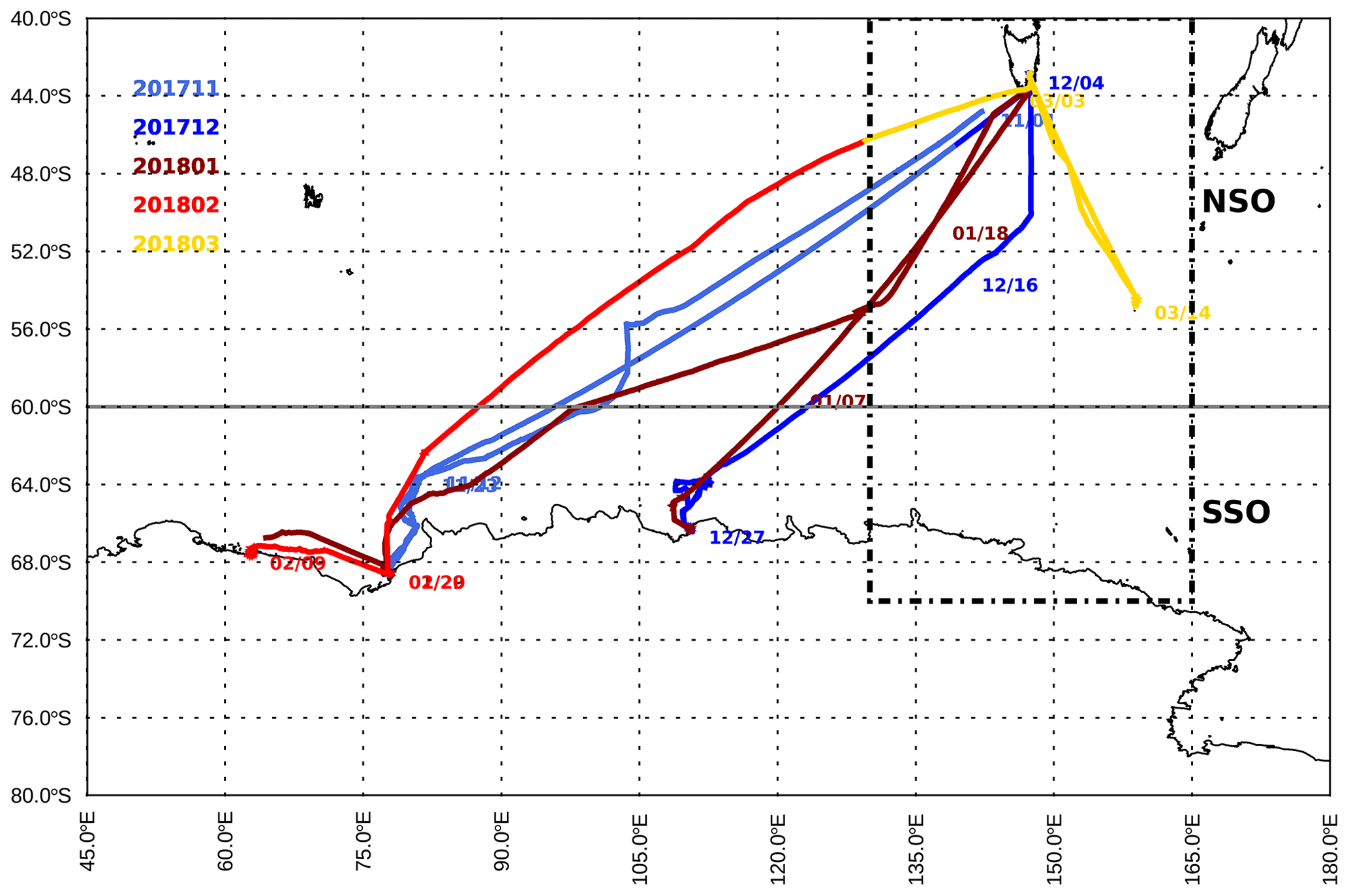
Figure 1 Ship track measurements between Hobart, Australia, and Antarctica. Different colors represent a different month's ship tracks, from 29 October 2017 to 23 March 2018, during MARCUS. Along the ship tracks, the study domain is separated into northern (NSO) and southern (SSO) parts of the Southern Ocean, with a demarcation line of 60^∘ S in order to study the clouds over the midlatitudes (north of 60^∘ S) and polar region (south of 60^∘ S). The black dotted rectangle represents the SOCRATES study domain. Some of the dates are labeled along the ship tracks, indicating the direction of the ship.

MARCUS ship-based instruments include AMF2 cloud radar, lidar, a microwave radiometer, a micropulse lidar, radiosonde sounding, a precision solar pyranometer, and a precision infrared radiometer, as well as aerosol sensors. Through these comprehensive observations over the SO, we are tentatively answering the following three scientific questions:

1. What is the total cloud fraction over the SO during MARCUS and the vertical and meridional variations in cloud fraction?

2. What are the dominant cloud types over the SO, their associated cloud phase and macrophysical properties, and their vertical and meridional distributions?

3. What are the vertical and meridional distributions of the low-level clouds over the SO?

This paper is organized as follows: the data and method are introduced in Sect. 2. The statistical results for all clouds during MARCUS are summarized in Sect. 3. The low-level cloud phase and macrophysical properties are described in Sect. 4, followed by a summary and conclusions in Sect. 5.

2 Data and method

2.1 Ship-based measurements used in this study

The AMF2 instruments, measurements, and their corresponding uncertainties and references are listed in Table 1. Because AMF2 was designed to support shipboard deployments, the baseline suite of instruments are marine-focused, including the 95 GHz W-band Atmospheric Radiation Measurement (ARM) user-facility Cloud Radar (WACR), ceilometer, micropulse lidar (MPL), microwave radiometer (MWR), aerosol observation system (AOS), meteorological measurements (MET, which includes the following data: temperature, pressure, specific humidity, and wind direction and speed) on the ship, rain gauge, and the radiosonde soundings. The combined cloud radar and ceilometer measurements can provide the cloud boundaries as long as there are no optically thin clouds and the cloud base heights (H_base) are not greater than the upper limit (7.7 km) of the ceilometer. The micropulse lidar will be used to identify optically thin clouds and the clouds with H_base>7.7 km. A previous study has shown that these additional clouds detected by the micropulse lidar can be a non-negligible supplement to the total cloud fraction (Mace et al., 2021). A detailed description of the instruments and the cloud parameters during MARCUS can be found in Mace et al. (2021) and McFarquhar et al. (2016, 2021).

Table 1 ARM AMF2 instruments and their corresponding measurements and uncertainties used in this study.

The cloud occurrence frequency can be determined through the following two steps: the column cloud fraction is simply the ratio of cloudy samples to the total observations every 5 min, and the occurrence frequency for each type of cloud during the entire time period equals the ratio of the number where the column cloud fraction is greater than zero for the total 5 min samples. In order to accurately estimate the cloud temperatures, we adopted a linear interpolation method based on the daily balloon soundings (4 to 5 times per day) to achieve a better temporal resolution of the vertical profiles of temperature, pressure, and specific humidity. The method considers MET measurements to ensure vertical continuity and adjacent soundings for temporal continuity. Using these interpolated atmospheric profiles, cloud temperatures can be obtained at a 5 min temporal resolution.

The cloud liquid water path (LWP) and atmospheric precipitable water vapor (PWV) are retrieved based on a physical-iterative algorithm using observations of the microwave radiometer brightness temperatures at 23.8 and 31.4 GHz, with uncertainties ranging from 15 to 30 g m⁻² (Marchand et al., 2003). It is important to note that the brightness temperature biases switch signs among different climatological regions because a threshold of 5 ^∘C in the cloud base temperature was used in their physical retrievals. Since the retrieved LWP and PWV are based on the MWR measured brightness temperatures at two frequencies, any biases in the brightness temperatures will affect these retrievals. Therefore, we propose an extra step to determine the uncertainties during MARCUS. Based on the temperature profiles, we can identify clouds that are not likely to contain liquid (e.g., pure ice cloud), and then we can estimate the LWP uncertainty based on their corresponding retrieved LWP values. From the probability density function (PDF_analysis), the LWP uncertainty is estimated as 10 g m⁻² for MARCUS.

To determine the precipitation status, the AOS and rain gauge measurements were used to determine whether rain is reaching the surface qualitatively, but not quantitatively, in this study. All the measurements were averaged over 5 min, except the radar reflectivity, Doppler velocity, and spectrum width used in Sect. 4.3.

2.2 Cloud type classification and single-layer, low-cloud phases

A classification method developed in Xi et al. (2010) was used to categorize different types of clouds using ARM radar–lidar-estimated cloud base (H_base) and top (H_top) heights and cloud thickness (ΔH). A brief description of the classification of cloud types is as follows (Table 1 and Fig. 6 in Xi et al., 2010). The single-layered, low-level clouds (LOW) are the fraction of time when low clouds with H_top≤3 km occur without clouds above them. Middle clouds (MID) range from 3 to 6 km, without any clouds below and above, while high clouds (HGH) have H_base>6 km, with no cloud underneath. Other types of clouds are defined by different combinations of the above three types, including middle over low (MOL), high over low (HOL), and high over middle (HOM), and the cloud column through the entire troposphere is defined as HML. The three types, MOL, HOM, and HML, include both contiguous and non-contiguous cloud layers, and their thicknesses may be overestimated when clear layer(s) are present between any two cloud layers.

Furthermore, we used the measurements of interpolated sounding, microwave- radiometer-retrieved LWP, radar reflectivity, Doppler velocity, and spectrum width to classify the cloud phase in each radar range volume of low-level clouds during MARCUS. The detailed classification method will be introduced in Sect. 4.1. We also used ERA-Interim reanalysis data to study the environmental conditions during MARCUS. The lower tropospheric stability (LTS) is calculated from the potential temperature difference between the surface and 700 hPa to assess the boundary layer stabilities when the low-level clouds appeared along the ship tracks. The relative contributions of mixed-phase, liquid, and ice clouds to the single-layered, low-level clouds, as well as their drizzling status, are also analyzed in this study. The latitudinal and longitudinal variations in the single-layered, low-level clouds and their vertical distributions are further explored in this study.

3 Statistical results for all clouds during MARCUS

The occurrence frequencies of total cloud cover and different types of clouds and their associated properties over the entire study domain during MARCUS are presented in Figs. 2–4. In order to examine the cloud properties over the midlatitude and polar regions, we separate the SO domain into northern (NSO; north of 60^∘ S) and southern (SSO: south of 60^∘ S) parts using a demarcation line of 60^∘ S. A total of 2447 h of cloud samples were collected during MARCUS in this study, of which 1181 h of the samples were located in the NSO and 1266 h of the samples were collected from the SSO. It is important to note that adding micropulse lidar measurements increased the total samples of non-liquid-containing clouds by ∼20 % because micropulse lidar is more sensitive to optically thin clouds than cloud radar. However, micropulse lidar signals are usually attenuated and cannot provide a meaningful signal when the liquid cloud layer is thicker than a couple of hundred meters (Sassen, 1991).

Figure 2 shows the vertical distributions of total cloud cover over the entire domain and over NSO and SSO. For the vertical distributions, the occurrence frequencies of total cloud increase from the first radar gate (∼226 m) to ∼700 m and then monotonically decrease with altitude, with a few small increments at different levels, especially over SSO. Comparing the occurrence frequencies of total cloud between NSO and SSO, we can draw the following conclusions. (1) The SSO has more cloudiness than the NSO under 7 km, while the NSO has more cloudiness than the SSO above 7 km. (2) Below 3 km, the occurrence frequencies of clouds over the NSO decrease dramatically from 37 % at an altitude of ∼700 m to 16 % at 3 km and from 45 % to 28 % over the SSO, which is similar to the vertical distributions of the low-level clouds over some Northern Hemisphere midlatitude regions, such as the eastern North Atlantic (ENA; Dong et al., 2014). The occurrence frequencies measured during MARCUS are much lower than those shown in Fig. 8 of Mace et al. (2009) throughout the entire vertical column between the same range of latitudes, especially as the occurrence frequencies during MARCUS are almost half of those measured by CloudSat and CALIPSO from 1 to 3 km. The reason has been explained in Xi et al. (2010); that is, a comparison of occurrence frequencies between the measurements of two different platforms can only be performed under an equivalent spatiotemporal resolution. In other words, our results were calculated under a 5 min temporal resolution, and the results in Mace et al. (2009) were statistically retrieved from the 2^∘ grid box. Therefore, a comparison between these two results is not reasonable. To make a fair comparison, one has to know the cloud amount at each area or time step, and then the product of amount and frequency is independent of either temporal and spatial measurement.

Figure 2 Mean vertical distributions of total clouds derived from ARM radar–lidar observations with a 5 min temporal resolution and a 30 m vertical resolution during MARCUS.

To compare with other studies, we calculated the cloud fractions (CFs) of total and different types of clouds. The total CFs were 77.9 %, 67.6 %, and 90.3 % for the entire domain, NSO, and SSO, respectively, indicating that 22.7 % more clouds occurred in the polar region than in the midlatitude region. The total CF over the entire domain is very close to the 76 % calculated by Mace and Protat (2018), who used ship-based measurements during the Cloud, Aerosols, Precipitation, Radiation and Atmospheric Composition over the Southern Ocean (CAPRICORN) field experiment. The total CF over the SSO is close to that estimated by using the complementarity of Cloud-Aerosol Lidar with Orthogonal Polarization (CALIOP) lidar aboard Cloud-Aerosol Lidar and Infrared Pathfinder Satellite Observation (CALIPSO) and the Cloud Profiling Radar (CPR) aboard CloudSat (DARDAR version 2 data) from Listowski et al. (2019).

Figure 3 shows the occurrence frequencies of categorized clouds and their cloud boundaries using the maximum H_top and the minimum H_base if there are two or more layers in each 5 min sample. For example, the mean H_base and H_top for single-layered, low-level (LOW) clouds are 0.92 and 1.62 km, respectively, listed in Table 2, which are the average values of min H_base and max H_top in the LOW category. As illustrated in Fig. 3a, the single-layered, low-level (LOW), deep cumulus or multilayered (HML), and MOL clouds are the three dominant types of clouds over the SO. Comparing the clouds between NSO and SSO, all types of clouds in SSO have a higher frequency of occurrence than those in NSO, except for HOL. The differences range from less than 1 % (LOW) to more than 10 % (MOL). Comparing the clouds over midlatitude oceans between the two hemispheres, i.e., between the NSO and ARM ENA site (Dong et al., 2014), we find the following: (1) the total cloud fractions (CFs) are close to each other (67.6 % over NSO vs. 70.1 % at ARM ENA), (2) LOW CFs are 22.9 % vs. 27.1 %, which is the dominant type of cloud in both regions, and (3) both MOL and HML clouds, including underneath low clouds, are 14.2 % and 16.5 % over NSO, much higher than those (4.2 % and 12.1 %) at ARM ENA site, indicating that there are more MOL and deep convective clouds over NSO than over ENA.

Figure 3 (a) Occurrence frequencies of categorized clouds by their vertical structures. LOW refers to single-layered low clouds (H_base and H_top≤3 km). MID refers to single-layered middle clouds (H_base>3 km  and H_top≤6 km). MOL refers to MID over LOW (H_base<3 km and H_top≤6 km). HGH refers to single-layered high clouds (H_base>6 km). HOM refers to HGH over MID (3 km $<H_{\mathrm{base}}<\mathrm{6}$ km and H_top>6 km). HML refers to HGH over MID and LOW (H_base<3 km and H_top≥6 km with a MID layer). HOL refers to HGH over LOW (LOW and HGH appear at the same time). (b) Cloud thickness for each type of cloud is shown with bars. The tops and bottoms of the bars represent the maximum cloud-top and minimum cloud base heights, respectively. Black, blue, and red bars represent the entire domain (lat. 41–69^∘ S, long. 60–160^∘ E), north of 60^∘ S (NSO), and south of 60^∘ S (SSO), respectively, during the MARCUS field campaign (October 2017–March 2018).

Table 2 Mean, standard deviation, minimum and maximum cloud base heights (H_base), cloud-top heights (H_top), and LWPs (all samples, single layered, and multilayered) of all seven types of clouds over the SO. All cloud heights have units in kilometers, and LWP has a unit of grams per square meter (g m⁻²).

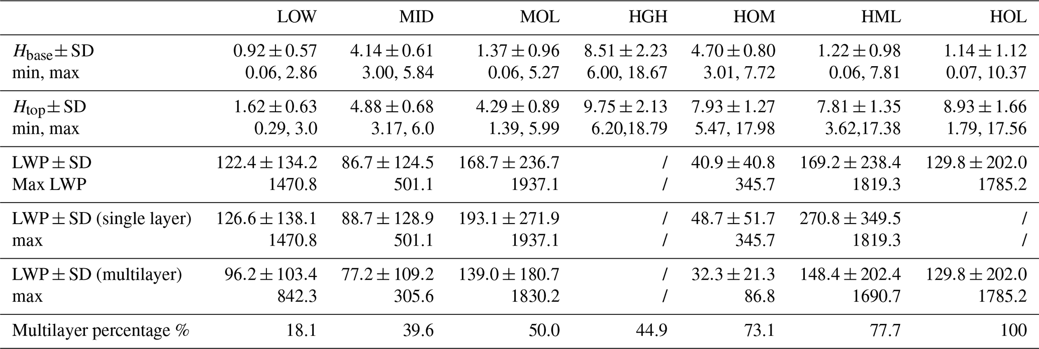
Figure 3b shows the vertical locations of different types of cloud layers, which represent the mean H_top and H_base listed in Table 2 for any type of cloud. Nearly all H_top and cloud thickness (ΔH) values over NSO are higher or deeper than those over SSO, presumably due to stronger solar radiation and stronger convection over NSO. H_base values basically followed their cloud-top counterparts, with a couple of exceptions. These cloud macrophysical properties are closely associated with large-scale dynamic patterns and environmental conditions. By analyzing the ERA-Interim reanalysis (not shown), the 850 hPa geopotential heights show persistent westerlies with slightly higher geopotential heights over the northwestern corner of the domain, which may closely relate to the higher H_top over NSO than over SSO. Furthermore, the boundary layer over NSO is relatively more stable than over SSO, based on lower troposphere stability (LTS) analysis (12.2–15.32 K over NSO vs. 11.48–13.29 K over SSO).

When we plot the probability density functions (PDFs) of cloud LWPs for different types of clouds, we find that the PDFs of LWPs for HGH and HOM peak are less than 10 g m⁻². These results make physical sense because HGH clouds should not contain any liquid droplets, and most HOM clouds, especially those over SSO, should be ice-phase dominant. In addition, the 10 g m⁻² of LWP is close to the uncertainty of the LWP retrieval in Marchand et al. (2003). Therefore, this value is used as a threshold for all types of clouds, which leads to less than 1 % reduction in the total samples. As shown in Fig. 4a, the LWPs (>10 g m⁻²) for all types of clouds are much higher over NSO than over SSO because the low-level and MOL clouds in the midlatitudes contain more liquid water than those in polar regions. The mean LWPs for liquid containing low-level and middle-level clouds over NSO, i.e., LOW, MID, and HOL, range from ∼130 to 150 g m⁻², while the mean LWPs for MOL and HML are 2 times higher (∼270 g m⁻²) than the mean LWP of LOW, MID, and HOL. Note that the mean LWPs for most types of clouds over the SSO are much lower than those over the NSO, except for the LOW clouds.

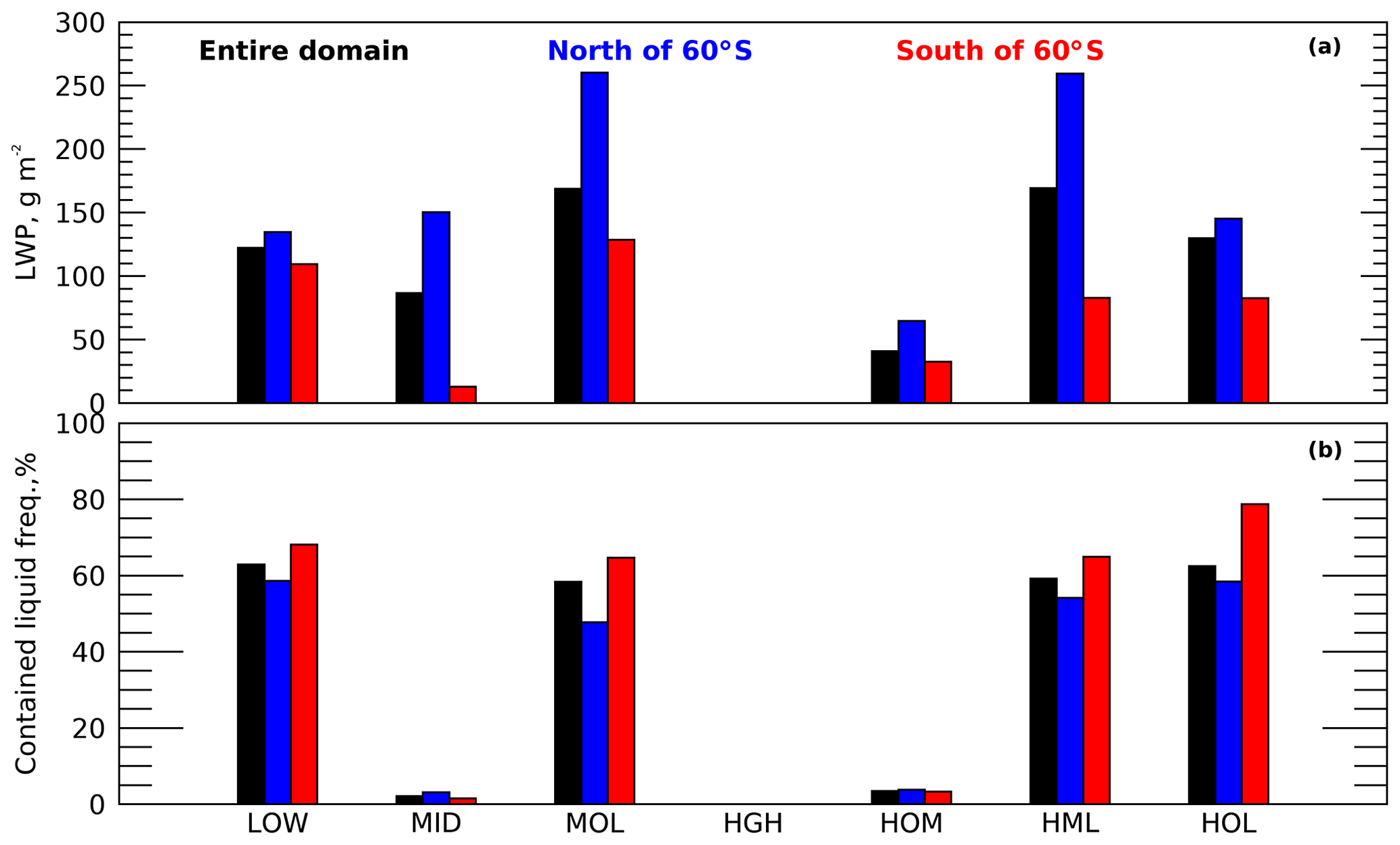
Figure 4 (a) Cloud liquid water paths (LWPs) retrieved from microwave radiometer (MWR) measured brightness temperatures using a physical retrieval method for each type of cloud. (b) The occurrence frequencies of LWPs >10 g m⁻² for each type of cloud.

The occurrence frequencies of LWPs (>10 g m⁻²) over NSO and SSO contradict their cloud LWP values, as demonstrated in Fig. 4b. To further investigate the amount of available precipitable water vapor (PWV), we found that mean PWV values in SSO are at least 2 to 3 times less than those in NSO for the same types of clouds (figure not shown). Note that the samples of MID, HGH, and HOM clouds are excluded from this study when they have LWPs less than 10 g m⁻², since these low LWPs are within the retrieval uncertainty of cloud LWP and hence may not contain any liquid cloud droplets. The higher LWPs, larger cloud droplets, drizzle drops and ice particles, and greater drizzling occurrence frequencies over NSO (discussed later) will lead to the quick dissipation of clouds over NSO. In contrast to NSO, the SSO cloud LWPs and particle sizes are much smaller, with fewer drizzling events, which increases cloud lifetime relative to NSO. The 67.6 % and 90.3 % CFs over NSO and SSO provide strong evidence for this argument. We can draw the following conclusions by comparing the cloud macrophysical properties between NSO and SSO in Figs. 3 and 4. The LOW fraction, thickness, and LWP over NSO and SSO are comparable to each other. For other types of clouds, cloud thicknesses are similar to each other or slightly deeper over NSO, but the cloud LWPs over NSO are much larger than those over SSO, resulting in more precipitation events over NSO. As pointed out in Albrecht (1989), more precipitation events may reduce the cloud lifetime. This argument is consistent with the results shown in Figs. 2 and 3a for all clouds, except for HOL. Cloud lifetimes over NSO are shorter than those over SSO, which leads to lower CFs over NSO than over SSO.

Table 2 provides a summary of the mean, standard derivation, and minimum and maximum for cloud boundaries, the LWP, and the percentage of multilayered clouds for each cloud type over the SO. Non-contiguous (multilayer) clouds over the SO occur very frequently, especially for HOM and HML. The LWP for single-layered clouds is greater than that for multilayered clouds. The LWP for single-layered HML almost doubles that for multilayered HML.

4 Single-layered, low-level clouds

As discussed in Sect. 3, single-layered, low-level clouds (LOW) are the dominant cloud type in both the northern (NSO) and southern (SSO) parts of the SO. Figures 3 and 4 further reveal that the LOW cloud type is the only one having comparable CF, cloud, thickness, and LWP over both NSO and SSO. This warrants further study – are the cloud phases, properties, and vertical and meridional variations of LOW clouds over these two regions similar to each other or significantly different?

4.1 Cloud phase

In this study, cloud boundaries are determined by combining cloud radar, ceilometer, and micropulse lidar measurements at a temporal resolution of 5 min. The cloud phase, liquid water droplets, or ice particles are determined in each radar range volume. A flow chart for classifying the phases of single-layered, low-level clouds is shown in Fig. 5. The determination of warm liquid clouds is straightforward using both cloud base (T_base) and cloud-top (T_top) temperatures greater than 0 ^∘C, and cloud LWPs greater than the threshold (10 g m⁻²). The determination of supercooled liquid clouds is slightly complicated. When either T_base or T_top is below 0^∘ C, and cloud LWPs are greater than the threshold, then the radar Doppler spectrum width (WID) and velocity (V_d) are used for the determination of supercooled liquid water clouds. If the majority (10 s of original radar measurements) of WID within a 5 min period are less than 0.4 m s⁻¹ and V_d are equal to or less than 0.0 m s⁻¹ (updrafts) in the volume, then this range volume is defined as supercooled liquid clouds.

Figure 5 A flow chart for phase classification of single-layered, low-level clouds. W-band (95 GHz) ARM Cloud Radar (WACR) provides radar spectrum width (WID) and Doppler velocity (V_d).

Mixed-phase clouds are determined when the median (calculated from 10 s of original radar measurements) of WID is greater than 0.4 m s⁻¹ or V_d is greater than 0.0 m s⁻¹ (downdrafts) due to the existence of large ice particles in the clouds. If cloud LWP is below the threshold, then it is defined as an ice cloud; otherwise, it is defined as a mixed-phase cloud. It is worth mentioning that large ice particles, which grow through vapor deposition or rime processes, dominate the radar reflectivity and are heavier than cloud droplets. Therefore, these large ice particles not only broaden the spectrum width but also have relatively large fall speeds.

To further evaluate our classification method, we compared the classified mixed-phase and ice clouds with the micropulse lidar linear depolarization ratios (LDRs) as an extra measure. The LDR ranges follow the method in Shupe et al. (2005), which are $\mathrm{0.11}<\text{LDR}<\mathrm{0.15}$ for mixed-phase clouds and LDR >0.15 for ice clouds, as listed in Table 1. Table 3a shows the quantitative comparison of the cloud-phase identifications between these two classification methods. The numbers represent the counts of each matched 5 min sample, where the diagonal numbers indicate that both methods are identifying the same type of cloud phase. In general, the two methods have 89 % agreement on the phase identification. Second, we performed the phase classification directly from microphysical probes on board the G-1 aircraft during SOCRATES and treated them as ground truth (Mohrmann et al., 2021). Since the in situ cloud microphysical measurements can tell us the phase of the cloud, the measurements allows us to see the percentage variations in cloud phase, by changing integration time of in situ sampling to mimic what the radar may observe the cloud for each range volume. Table 3b shows possible cloud phase partitionings that may be detected by cloud radar. As sampling time increases from 1 to 30 s, more mixed-phase clouds and fewer single-phase clouds can be observed.

Table 3 (a) Comparison of cloud phase identifications between our classification method and the Shupe et al. (2005) method in 5 min measurements each. The unit is number of 5 min samples. Numbers denote the cloud sample classifications between the two methods. For example, the number 98 denotes that a total of 98 samples are classified as mixed phase using the method in Shupe et al. (2005), while the rest are classified as liquid using this study's method. (b) The cloud phase partitioning from the Cloud Droplet Probe (CDP) and the Two-Dimensional Stereo Probe (2DS) during SOCRATES. Note that the CDP measures particle sizes from 2 to 50 µm in diameter, and the 2DS measures particle sizes from 50 to 5000 µm in diameter.

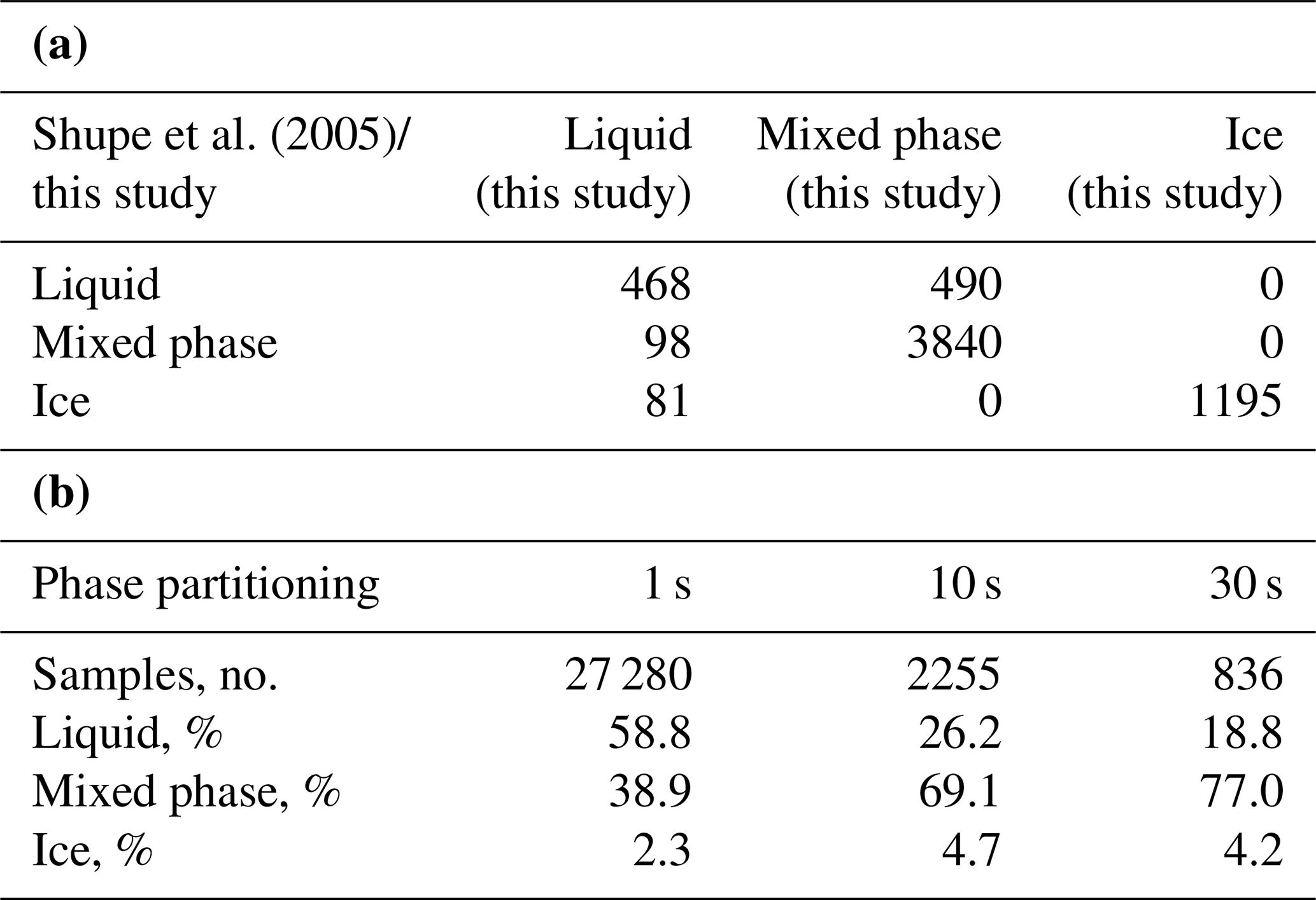
Figure 6 shows the determination of mixed-phase and ice clouds through combined measurements of radar reflectivity and spectrum width, lidar LDR and backscatter, and cloud LWP. For the classified ice clouds, cloud LWPs are lower than 10 g m⁻² (Fig. 6f), most of the Doppler spectrum widths range from 0.08 to 0.16 m s⁻¹ (Fig. 6b), and the LDR ratios (Fig. 6d) can be greater than ∼0.15, representing a narrow range of ice particle size distribution with higher LDR ratios. For the classified mixed-phase clouds, cloud LWPs are greater than 10 g m⁻², and most of the Doppler spectrum widths range from 0.15 to 0.5 m s⁻¹, representing a broad particle size distribution resulting from the mixture of liquid droplets and ice particles. An interesting result occurs where both LDR signals (>0.2) and LWPs are much higher during the drizzling periods (Fig. 6a), indicating a mixed-phase cloud with cloud droplets within the cloud layer and large liquid drizzle drops and ice crystals below cloud base.

Figure 6 A case study that shows our phase classification (a, b, c) and micropulse lidar (MPL) linear depolarization ratios (LDRs) and backscatter. W-band (95 GHz) ARM Cloud Radar (WACR) reflectivity is shown in panel (a), and spectrum width is shown in panel (b). Correspondingly, the phase classification is shown in panel (c), the MPL LDR is shown in panel (d), backscatter is shown in panel (e), and MWR-derived LWP is shown in panel (f).

Based on the Doppler velocity, the mode values for both mixed-phase and ice clouds occur at ∼0.5 m s⁻¹, where the ice particles are dominant in both types of clouds. The broader particle size distribution with lower LDR ratios for mixed-phase clouds and narrower particle size distribution with higher LDR ratios for ice clouds further corroborate that the classified results from this study are consistent with the traditional micropulse lidar LDR method.

It is important to note that the micropulse lidar signals are usually attenuated and cannot provide a meaningful signal when the liquid cloud layer is thicker than a couple of hundred meters (Sassen, 1991). Arctic mixed-phase clouds are typical with the liquid-dominant layer on the top of the mixed-phase clouds and the ice-dominant layer underneath. The ceilometer-derived cloud base height represents the base of the liquid-dominant layer near the cloud top, while the MPL-derived cloud base height represents the base of the lower ice-dominant layer (Qiu et al., 2015; Shupe, 2007; Shupe et al., 2005). Over the Arctic, the micropulse lidar signals can penetrate through the ice-dominant layer to the liquid-dominant layer. However, the mixed-phase clouds over the Southern Ocean are totally different from those over the Arctic region because they are well mixed (liquid droplets and ice particles) from cloud base to cloud top, which is found in this study. Thus, the micropulse lidar signals can be attenuated in the mixed-phase clouds over the Southern Ocean. Statistical results show that 43 % of micropulse lidar signals were attenuated during MARCUS compared to our classified results.

This classification method is further supported by the on-board cloud radar measurements during the Southern Ocean Clouds, Radiation, Aerosol Transport Experimental Study (SOCRATES; not shown). In that campaign, the reflectivity measurements were usually greater, and the spectrum widths were much wider when the aircraft observed large ice particles compared to the time periods when liquid cloud droplets were observed. Although the wider spectrum widths might be caused by Doppler broadening of the moving aircraft, further analysis shows that the on-board radar sends the signals (assuming the time of transmitted and received signals is short enough comparing to aircraft speed) in the perpendicular to the movement of the aircraft; that is, there is no relative movement between radar signals and clouds. Thus, the on-board radar spectrum width measurements should be not significantly impacted by Doppler broadening (relative movement in the same direction).

In this study, a total of 6934 5 min single-layered, low-level cloud samples were determined using our classification method, including 697 liquid cloud samples, 3777 mixed, 1205 ice, and 1255 other clouds. The category of other clouds represents more than one phase in each column. Note that although other also refers to a mixed-phase cloud, it has different vertical distribution of liquid compared to the mixed cloud. It is also worth mentioning that about 5.5 % of single-layered, low-level cloud phases could be determined when the radar measurements were not available during MARCUS, and those were not accounted to the category of other clouds.

Figure 7a shows the drizzling status for each categorized cloud type, i.e., no rain (green), virga (brown), and rain (navy blue). The definition of drizzling status follows the method in Wu et al. (2015, 2017), where there are radar reflectivity measurements below the ceilometer-/lidar-determined cloud base. The major difference for drizzle in the studies of Wu et al. (2015, 2017) and this study is that drizzle is in the liquid phase at the ARM ENA site but could be both liquid and ice phases in this study.

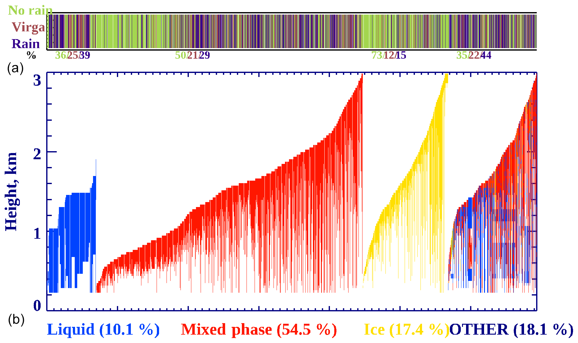
Figure 7 (a) The drizzling status for each categorized cloud type, e.g., no rain (green), virga (brown), and rain (navy blue). The percentages shown below the x axis represent the portion of drizzling in each type of cloud. (b) The percentages and vertical distributions of classified liquid, mixed-phase, ice, and other clouds for each column in the single-layered, low-level clouds, represented by different colors, over the entire domain during MARCUS. Each line represents one 5 min sample. The definition of drizzle here is the radar reflectivity below the ceilometer-derived cloud base, which could be either liquid drizzle drops or ice crystals.

The percentages shown below the x axis represent the portion of drizzling status in each type of cloud, such as liquid, mixed-phase, ice, and other clouds. Figure 7b also shows the percentages and vertical distributions of classified liquid, mixed-phase, ice, and other clouds for each column in the single-layered, low-level clouds, represented by different colors. After classification, the samples in each category are sorted by their H_top. In detail, Fig. 7 demonstrates that the mixed-phase clouds dominate the single-layered, low-level cloud category with an occurrence frequency of 54.5 %. The other and ice clouds have similar occurrence frequencies of 18.1 % and 17.4 %, respectively, while the liquid clouds have the lowest occurrence frequency of 10.1 %. The liquid-topped mixed-phase clouds (included in other), which frequently occur in the Arctic region (Qiu et al., 2015), are rarely found over the SO. The existence of ice particles in mixed-phase clouds should strongly depend on the distribution of ice nuclei (IN), whereas spatially unevenly distributed IN may result in the other type of cloud.

Based on the results in Fig. 7, we draw the following conclusions. Most of the ice clouds are without icy precipitation, and the percentages with virga and precipitation below the cloud base are 12 % and 15 %, respectively. The percentages of non-drizzling, virga, and drizzling mixed-phase clouds are 50 %, 21 %, and 29 %. The liquid and other clouds have similar percentages; they are 36 %, 25 %, and 39 % for liquid clouds and 35 %, 22 %, and 44 % for other clouds. For liquid and other clouds, the drizzling frequencies are independent of H_top. In contrast, for mixed-phase and ice clouds, the drizzling frequencies strongly depend on H_top, i.e., higher drizzling frequencies occur mostly at higher H_top.

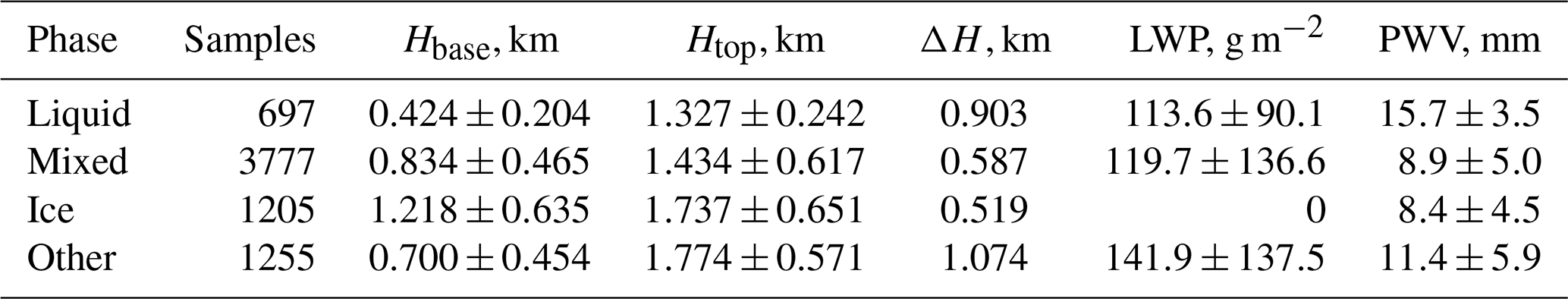
The properties of single-layered, low-level clouds are summarized in Table 4. The liquid clouds have the lowest H_base and H_top but more available water vapor than other types of clouds. Since the other clouds are a transitional stage among mixed-phase, liquid, and ice clouds, they have the highest H_top, deepest cloud layer, and largest LWP. The ice clouds occur in relatively dry environments and have the highest H_base at 1.218 km and thinnest cloud layer. The cloud variables for mixed-phase clouds fall between liquid and other. Since LWPs in mixed-phase clouds have a larger standard deviation, which implies that SLW is more common at higher LWPs and ice is more common at lower LWPs.

Table 4 Liquid, mixed, ice and other phases of cloud properties within the single-layered, low-level clouds.

4.2 Meridional variations in cloud properties

Figure 8 shows the meridional variation in single-layered, low-level cloud properties during MARCUS. As illustrated in Fig. 8a, the meridional distributions of H_base, H_top, and ΔH are nearly independent of latitude; however, their corresponding temperatures (T_base and T_top) increased by about 8 K from 69 to 43^∘ S, although there were slight fluctuations. These results suggest that the cloud and sea surface temperatures have minimal impact on the cloud boundaries over the SO, which is consistent with the findings in McFarquhar et al. (2016). The meridional variation of LWPs follows those of T_base and T_top, with an increasing trend from south to north. It is important to point out that a big drop in LWP at ∼50^∘ S results from fewer occurrences of low-level clouds there, indicating that the cloud samples at some latitudes are not statistically significant. The atmospheric PWV increased dramatically from ∼5 mm at 69^∘ S to ∼18 mm at 43^∘ S, presumably due to increased sea surface and atmospheric temperatures.

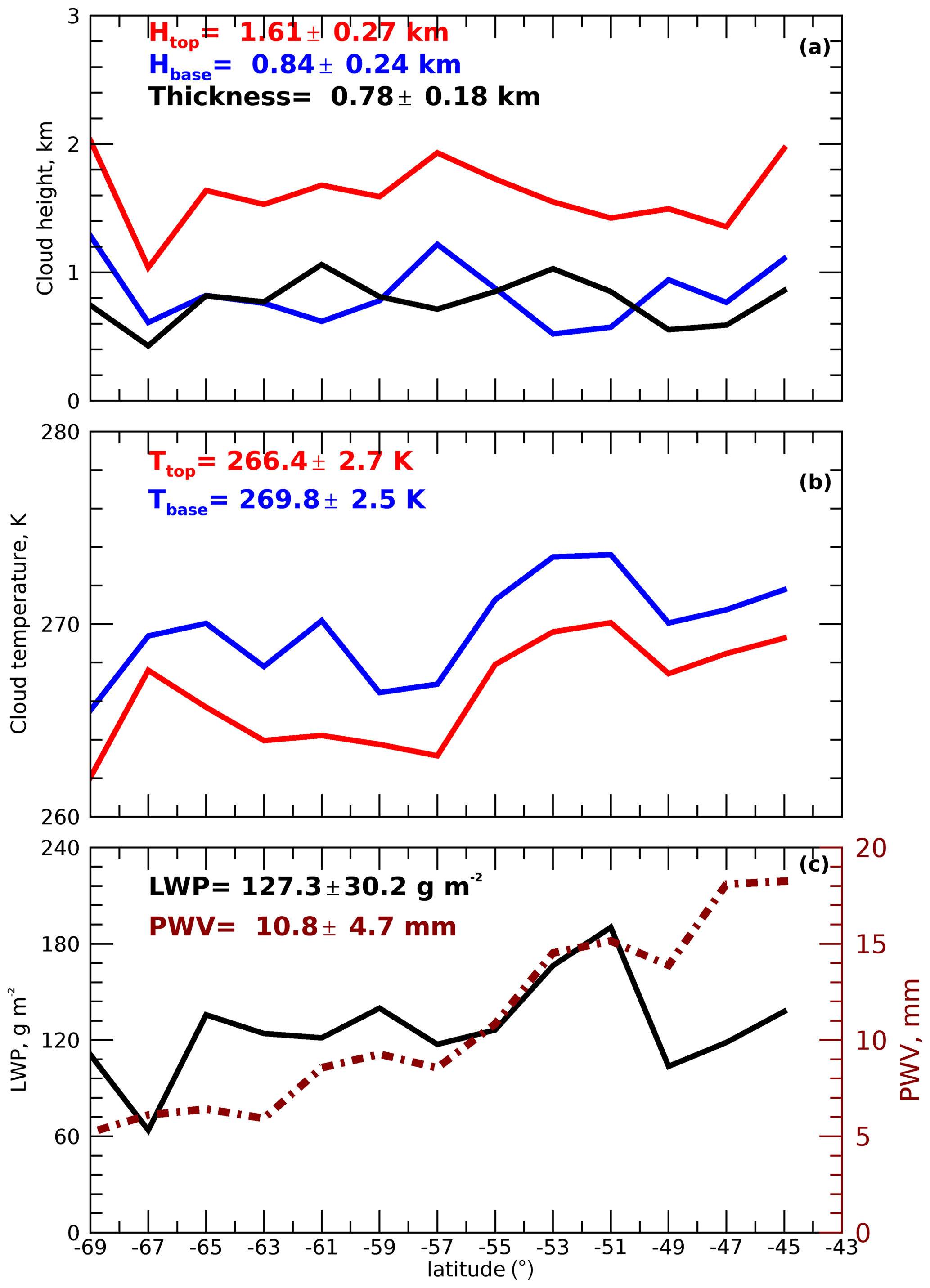
Figure 8 Meridional variations in single-layered, low-level cloud properties. (a) Cloud base (H_base) and cloud-top (H_top) heights and cloud thickness (ΔH). (b) Cloud base (T_base) and cloud-top (T_top) temperatures. (c) Cloud liquid water path (LWP) and precipitable water vapor (PWV) over the entire domain during MARCUS.

Figure 9 shows the latitudinal and meridional distributions of categorized liquid, mixed-phase, ice, and other in single-layered, low-level clouds over the SO during MARCUS. Each circle represents the exact location and time along the ship track. Mixed-phase clouds occurred everywhere over the SO during the MARCUS field campaign and became dominant in November, December, and February. Liquid clouds dominated in March, while ice clouds dominated in January. The other clouds are a kind of transitional phase falling in between the mixed-phase and ice/liquid clouds because there are no standalone occurrences in any month during MARCUS.

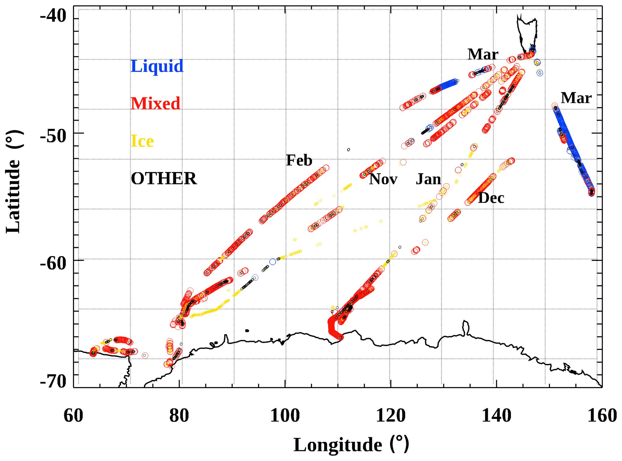
Figure 9 The latitudinal and longitudinal distributions of classified mixed-phase, liquid, and ice clouds in the single-layered, low-level clouds. The liquid (blue), mixed (red), ice (yellow), and other (black) values are shown along each ship track from October 2017 to March 2018 during MARCUS.

4.3 Vertical distribution of cloud properties

The vertical distributions of classified liquid, mixed-phase, and ice clouds in LOW category are presented in Figs. 10–12. The focus of this section will be comparisons of cloud macrophysical properties between the north (NSO) and south (SSO) regions of the domain. Figure 10a shows the vertical distributions of liquid clouds, which were capped at ∼1.6 km, mostly in the marine boundary layer. The vertical occurrence frequencies are up to 27 % over NSO, while they were less than 4 % over SSO, i.e., liquid clouds occurred fairly often over the midlatitude region, but very few occurred over the polar region. On the contrary, the occurrence frequencies of mixed-phase clouds between NSO and SSO are opposite to liquid clouds, as illustrated in Fig. 10b, although the differences are not so obvious. Mixed-phase clouds increased with altitude until ∼1.6 km and then decreased monotonically towards 3 km. The highest frequencies were ∼37 % at 0.6 km over SSO and ∼27 % at 1.5 km over NSO. The vertical distributions of ice clouds are similar to those of mixed-phase clouds (Fig. 10c); however, there were no significant differences between NSO and SSO. It is worth mentioning that the vertical distributions of mixed-phased clouds over SO are quite different to those from the DOE ARM North Slope of Alaska (NSA) site, where the low-level mixed-phase clouds are commonly featured with a liquid-topped layer (e.g., Qiu et al., 2015).

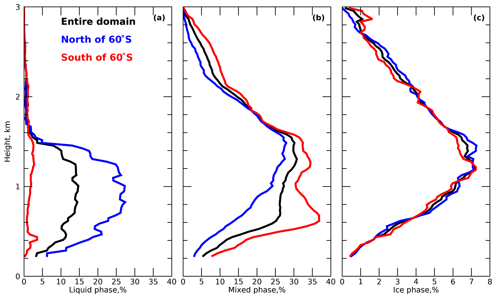
Figure 10 Occurrence frequencies of classified mixed-phase, liquid, and ice clouds over the entire domain (black), north of 60^∘ S (blue), and south of 60^∘ S (red) during MARCUS.

Figure 11 Normalized vertical distributions of radar reflectivity (a), Doppler velocity (b), and spectrum width (c) for the classified liquid (a–c), mixed-phase (d–f), and ice (g–i) clouds over the north of 60^∘ S during the MARCUS intensive observational period (IOP). Normalized height is defined as $=\frac{H-H_{\mathrm{base}}}{H_{\mathrm{top}}-H_{\mathrm{base}}}$, where the cloud base is denoted as 0 and cloud top is 1. The black lines represent the median values, and the white lines in Doppler velocity represent the reference of 0.0 m s⁻¹.

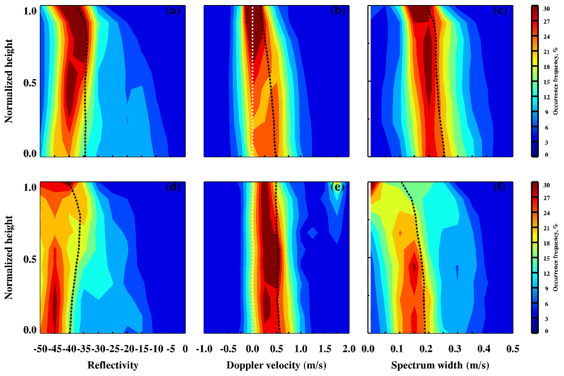
Figure 12 Same as Fig. 11 but only for mixed-phase (a–c) and ice (d–f) clouds over the south of 60^∘ S during MARCUS.

To further investigate the vertical distributions of classified liquid, mixed-phase, and ice clouds over NSO and SSO, we plot the normalized vertical distributions (cloud base as 0; cloud top as 1) of radar reflectivity, Doppler velocity, and spectrum width in Figs. 11 and 12, respectively. In this study, the threshold of −50 dBZ was used to determine the cloud boundary over the SO instead of the threshold of −40 dBZ radar reflectivity used at the ARM ENA site (Dong et al., 2014). If we used the threshold of −40 dBZ over the SO, then there would be only 73 % of cloud samples available. If we used the threshold of −50 dBZ, then we would have 90.4 % of cloud samples, which gained an additional 17.4 % on top of the −40 dBZ threshold. About 9.6 % of the radar reflectivities during MARCUS are lower than −50 dBZ for all LOW cloud samples but without ceilometer and MPL lidar signals. Thus, these 9.6 % cloud samples were eliminated in Figs. 11–12.

Figures 11a–c represent the normalized vertical distributions of the radar reflectivity, Doppler velocity, and spectrum width of liquid clouds. Liquid clouds had the lowest reflectivity near the cloud top because of cloud-top entrainment. The reflectivity had a nearly constant median value of $\sim -\mathrm{22}$ dBZ from cloud top height (∼0.8 for normalized height) of the cloud layer to the cloud base. Most of the reflectivities were less than −15 dBZ, which is a threshold to distinguish cloud droplets and drizzle drops in each radar range volume (Wu et al., 2020). Most of the Doppler velocities were greater than 0.0 m s⁻¹, indicating that downwelling motion is dominant in liquid clouds. The profiles of Doppler velocity and spectrum width increased smoothly from the cloud top to base, suggesting that larger cloud droplets and broader size distributions exist near the cloud base, which is attributable to more drizzle drops near the cloud base, as illustrated in Fig. 7.

The vertical distributions of mixed-phase clouds in Fig. 11d–f are similar to those of liquid clouds. The more occurrences of larger reflectivity measurements and larger median values of spectrum width near the cloud base are most likely due to the presence of moderate ice particles and/or drizzle drops. The nearly same median values of reflectivity, Doppler velocity, and spectrum width (but slightly larger standard deviations in each level in mixed-phase clouds) in both liquid and mixed-phase clouds suggest that the ice particle sizes in mixed-phase clouds are comparable to cloud droplets and drizzle drops. The nearly uniform vertical distributions of Doppler velocity and spectrum width indicate well-mixed liquid cloud droplets and ice particles throughout the cloud layer in the mixed-phase clouds over NSO.

Compared to liquid and mixed-phase clouds, ice clouds had much lower reflectivities and a narrower spectrum width, as shown in Fig. 11g–i. Almost all reflectivity measurements were less than −25 dBZ, with a median value of −35 dBZ at the cloud base, resulting from small or moderate ice particles but much lower concentration. A nearly constant Doppler velocity within the cloud layer further supports the discussion of mixed-phase clouds above, i.e., that the ice particle sizes are independent of cloud height and comparable to liquid cloud droplets in the low-level clouds over the SO. Because there are no mechanisms for growing large ice particles in such shallow ice clouds, the accretion process cannot take place. From the statistical results in Fig. 7, these ice particles have relatively little chance to become virga or raindrops and usually dissipate or transition to other types of clouds.

Since there are not enough liquid cloud samples over the polar region, only the mixed-phase and ice clouds results are shown in Fig. 12. Compared to the vertical distributions of ice clouds over NSO, the median values of reflectivity and Doppler spectrum width over SSO were lower and narrower, indicating a lack of large ice particles in the polar region. The small ice particles in the polar region were also reflected in their mixed-phase clouds. Compared to the vertical distributions of the mixed-phased clouds over NSO, the median values of reflectivity and Doppler spectrum width over SSO were dramatically lower (−35 dBZ at SSO vs. −22 dBZ at NSO; 0.25 m s⁻¹ at SSO vs. 0.32 m s⁻¹ at NSO). Figure 12 illustrates that the ice particle sizes over SSO are smaller and their size distributions are narrower than those over NSO, indicative of lack of large ice particles over SSO.

5 Summary and conclusions

In this study, we presented the statistical results of clouds over the Southern Ocean (SO) and its northern (NSO) and southern (SSO) parts during the MARCUS intensive observational period (IOP). We used the method developed in Xi et al. (2010) to calculate the occurrence frequencies of different types of clouds and their corresponding cloud macrophysical properties. We developed a new method to classify liquid, mixed-phased, and ice clouds in the single-layered, low-level clouds, as well as their corresponding drizzling status. Last, we explored the meridional and vertical distributions of these classified cloud properties. Analysis of the MARCUS cloud phase and macrophysical properties has yielded the following conclusions.

1. The total cloud fractions (CFs) were 77.9 %, 67.6 %, and 90.3 % for the entire domain, NSO, and SSO, respectively, indicating that 22.7 % more clouds occurred in the polar region than in the midlatitude region. The SSO had more clouds under 7 km, while the NSO had more clouds above 7 km. Below 3 km, the occurrence frequencies of clouds over NSO decrease dramatically from 37 % at an altitude of ∼0.7 km to 16 % at 3 km, which is similar to the vertical distributions of the low-level clouds over some Northern Hemisphere midlatitude regions, such as the eastern North Atlantic.

2. The single-layered, low-level (LOW), deep connective or multilayered (HML), and MOL clouds are the three dominant types of clouds over the SO. Comparing the clouds between NSO and SSO, all types of clouds in SSO are higher than those in NSO, except for HOL. The LOW fraction, thickness, and LWP over both NSO and SSO are comparable to each other. The mean LWPs for LOW, MID, and HOL clouds over NSO, range from ∼130 to 150 g m⁻², while the mean NSO LWPs (∼270 g m⁻²) for MOL and deep convective clouds (HML) are 2 times higher than the same types of clouds over SSO. The mean LWPs of clouds over SSO are much lower than the LWPs over NSO. Over the Southern Ocean, the single-layered or contiguous clouds usually have higher LWP than their counterparts of multilayered or non-contiguous clouds. There are more non-contiguous HML and HOM than contiguous ones.

3. A new method was developed to classify liquid, mixed-phase, and ice clouds in the single-layered, low-level clouds (LOW) based on comprehensive ground-based observations. The mixed-phase clouds are dominant in the LOW cloud category, with an occurrence frequency of 54.5 %. The other and ice clouds had similar occurrence frequencies of 18.1 % and 17.4 %, respectively, while the liquid clouds had the least occurrence frequency of 10.1 %. The percentages of non-drizzling, virga, and drizzling for mixed-phase clouds were 50 %, 21 %, and 29 %, and the drizzling frequencies of mixed-phase clouds strongly depend on H_top; that is, higher drizzling frequencies occurred mostly at higher H_top.

4. The meridional distributions of H_base, H_top and ΔH are nearly independent of latitude; however, their corresponding temperatures increased by about 8 K from 69 to 43^∘ S. The meridional variation in LWPs mimics that of cloud temperatures, with an increasing trend from south to north. The mean PWV increased dramatically from ∼5 mm at 69^∘ S to ∼18 mm at 43^∘ S due to increased sea surface and atmospheric temperatures. More liquid clouds occurred over NSO, but very few occurred over SSO, whereas more mixed-phase clouds occurred over SSO than over NSO. There were no significant differences in ice cloud occurrences between NSO and SSO.

The (nearly the same) median values of reflectivity, Doppler velocity, and spectrum width in both liquid and mixed-phase clouds over NSO suggest that the ice particle sizes in mixed-phase clouds are comparable to cloud droplets and drizzle drops. The uniform vertical distributions of Doppler velocity and spectrum width suggest well-mixed liquid cloud droplets and ice particles throughout the cloud layer in the mixed-phase clouds over NSO, which are quite different from those over the DOE ARM NSA site, where the liquid-topped mixed-phase low-level clouds are common. The median values of reflectivity and Doppler spectrum width over SSO were lower and narrower than those over NSO, indicating lack of large ice particles in the polar region.

These results provide comprehensive statistical properties of all clouds over the SO during MARCUS, including the occurrence frequencies of different types of clouds and their corresponding cloud macrophysical properties. We also examined the meridional and vertical distributions of the classified cloud properties. These statistics can be used as a ground truth to evaluate satellite-retrieved cloud properties and model simulations over the SO. The results of this study will help to advance our understanding of the clouds over the SO, which may lead to improved model simulations and a better representation of global climate.