The impact of sampling strategy on the cloud droplet number concentration estimated from satellite data

Cloud droplet number concentration (N_d) is of central importance to observation-based estimates of aerosol indirect effects, being used to quantify both the cloud sensitivity to aerosol and the base state of the cloud. However, the derivation of N_d from satellite data depends on a number of assumptions about the cloud and the accuracy of the retrievals of the cloud properties from which it is derived, making it prone to systematic biases.

A number of sampling strategies have been proposed to address these biases by selecting the most accurate N_d retrievals in the satellite data. This work compares the impact of these strategies on the accuracy of the satellite retrieved N_d, using a selection of in situ measurements. In stratocumulus regions, the MODIS N_d retrieval is able to achieve a high precision (r² of 0.5–0.8). This is lower in other cloud regimes but can be increased by appropriate sampling choices. Although the N_d sampling can have significant effects on the N_d climatology, it produces only a 20 % variation in the implied radiative forcing from aerosol–cloud interactions, with the choice of aerosol proxy driving the overall uncertainty. The results are summarised into recommendations for using MODIS N_d products and appropriate sampling.

1 Introduction

The droplet number concentration (N_d) is a key property of clouds. It is important for setting cloud and precipitation process rates (e.g. Khairoutdinov and Kogan, 2000) as well as cloud radiative properties (George and Wood, 2010; Painemal, 2018). It is closely related to the aerosol environment and the in-cloud updraught (Twomey, 1959), as well as being affected by precipitation processes (Wood, 2012) and entrainment (Baker et al., 1980). With this important role for cloud properties, N_d has been used to evaluate the performance of global climate models (Mulcahy et al., 2018; McCoy et al., 2020; Robson et al., 2020; Grosvenor and Carslaw, 2020).

Variations in N_d are also a primary method for observational characterisations of aerosol effects on clouds (e.g. Quaas et al., 2006). An increase in available cloud condensation nuclei (CCN) will typically produce an increase in N_d, which can result in changes in droplet size and cloud reflectivity (Twomey, 1974), modifications to precipitation processes (Albrecht, 1989), intensification of convection (Williams et al., 2002), and increases in evaporation and potential cloud desiccation (Wang et al., 2003; Ackerman et al., 2004). This has made aerosol relationships with N_d the target of a large number of observational studies (e.g. Quaas et al., 2006, 2008; Ghan et al., 2016; Gryspeerdt et al., 2017; McCoy et al., 2017; Hasekamp et al., 2019). With a central role in aerosol–cloud interactions, N_d relationships with other cloud properties, particularly cloud fraction (CF; Gryspeerdt et al., 2016) and liquid water path (LWP; Han et al., 2002), have also been used to quantify cloud adjustments due to aerosols.

Assessments of the effective radiative forcing due to aerosol–cloud interactions (ERFaci) rely heavily on these observation-based estimates of aerosol–cloud interactions (Boucher et al., 2013; Bellouin et al., 2020), and these estimates in turn rely on accurate observations of aerosol–N_d and N_d–cloud relationships. Reliable satellite and remotely sensed observations of N_d are therefore essential for reducing uncertainties in the anthropogenic impact on clouds and the climate.

There are a number of methods for retrieving cloud droplet size and N_d from space (Boers et al., 2006; Zeng et al., 2014; Austin and Stephens, 2001; Hu et al., 2021), but the majority of previous studies make use of the cloud droplet number calculated from a bispectral retrieval of the cloud optical depth (τ_c) and effective radius (r_e; Nakajima and King, 1990), assuming an adiabatic cloud (Boers et al., 2006; Quaas et al., 2006). Previous studies in stratocumulus regions have found a good agreement between the satellite and in situ N_d (Painemal and Zuidema, 2011; Kang et al., 2021), but this retrieval depends on assumptions with varying applicability (Grosvenor et al., 2018b). To improve our knowledge of N_d across the globe, a number of sampling strategies have been applied in recent work to select more reliable retrievals (Quaas et al., 2006; Grosvenor et al., 2018b; Bennartz and Rausch, 2017; Zhu et al., 2018), based on the characteristics of the retrieval and the observed liquid clouds.

Each of these sampling strategies is based on an understanding of cloud physics and the character and reliability of satellite retrievals such that it is not immediately clear which is most suitable for selecting valid N_d retrievals. In addition, as N_d products are used for a variety of different tasks, different sampling methods may be more appropriate for each. Removing low-optical-depth clouds may limit the N_d retrieval to more accurate cases but may produce a biased climatology and estimates of the ERFaci by neglecting a large fraction of the cloud population (Leahy et al., 2012). This work examines these sampling strategies and how the choices made impact the accuracy of the N_d retrieval when compared to in situ data, the representativeness of the N_d climatology and the impact of these choices on the implied aerosol–cloud radiative forcing.

2 Methods

2.1 N_d from satellite

N_d is rarely retrieved directly but is estimated from the cloud optical depth (τ_c) and effective radius (r_e). Assuming an adiabatic cloud (no precipitation or mixing with its environment), N_d is derived from the retrieved properties (τ_c, r_e) following Brenguier et al. (2000), Quaas et al. (2006) and Boers et al. (2006):

$$\begin{array}{}\text{(1)}& N_{\mathrm{d}}={\displaystyle \frac{\mathrm{1}}{\mathrm{2}\mathit{\pi }k}}\sqrt{{\displaystyle \frac{\mathrm{5}}{Q{\mathit{\rho }}_{\mathrm{w}}}}}{\left(f_{\mathrm{ad}}{c}_{\mathrm{ad}}\right)}^{\mathrm{1}/\mathrm{2}}{\mathit{\tau }}_{\mathrm{c}}^{\mathrm{1}/\mathrm{2}}{r}_{\mathrm{e}}^{-\mathrm{5}/\mathrm{2}},\end{array}$$

where the density of water ρ_w and the scattering efficiency Q (equal to 2) are assumed constant. $k=(r_{\mathrm{v}}/r_{\mathrm{e}}{)}^{\mathrm{3}}$, where r_v is the droplet mean volume radius, depends on the droplet size spectrum. Although k has been observed to vary in in situ studies (Martin et al., 1994) and it may vary under particularly extreme aerosol environments (Noone et al., 2000), this work uses a constant value of 0.8, following Painemal and Zuidema (2011) and Grosvenor and Wood (2014).

The condensation rate c_ad is a function of temperature and pressure. Assuming a saturated adiabatic lapse rate, the pressure dependence is weak, but a temperature change from 270 to 300 K can double the condensation rate and hence N_d. To account for this variation, N_d is calculated using the linear N_d temperature correction from Gryspeerdt et al. (2016), using the cloud top temperature (a suitable assumption if the cloud layers are thin;  Grosvenor and Wood, 2014).

The sub-adiabatic factor (f_ad) in Eq. (1) represents the reduction in the condensation rate due to mixing with sub-saturated environmental air. However, a full accounting for sub-adiabaticity also requires a potential change in the droplet size distribution (except under extreme inhomogeneous mixing), which modifies the k parameter. Previous work has suggested that there might be a cancellation between these two effects (Painemal and Zuidema, 2011). Observational studies have found a range of values for the adiabatic factor from 0.63 (Merk et al., 2015), 0.74 (Kang et al., 2021), 0.8 (Braun et al., 2018), 0.88 (Painemal et al., 2017) and 0.9 (Painemal and Zuidema, 2013). In this work a constant factor of 0.8 is used, noting that this may be responsible for an offset in the retrieved N_d.

2.2 Satellite sampling

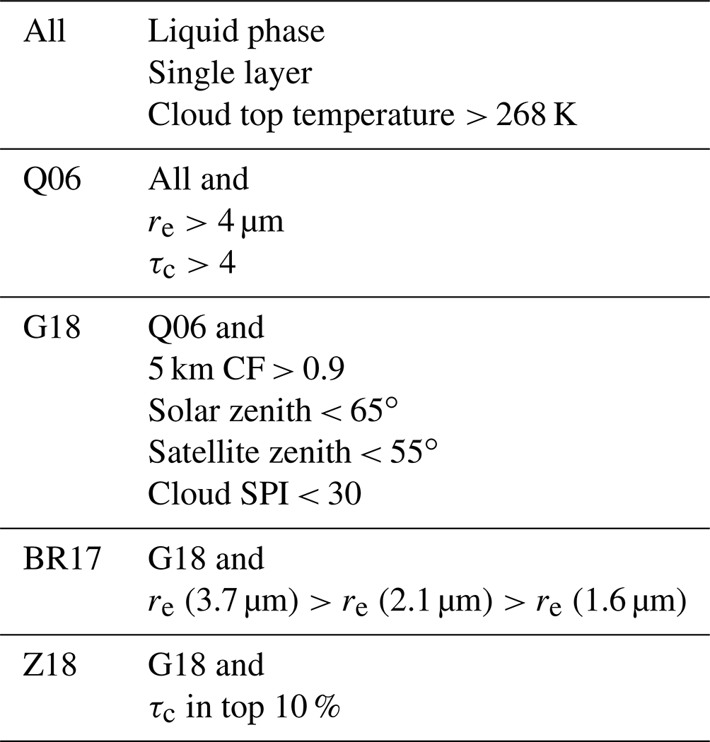
Two of the major uncertainties in the N_d retrieval are the cloud adiabaticity assumption and the accuracy of the cloud retrievals used to derive N_d. This work examines sampling strategies to minimise these uncertainties in the MODIS collection 6.1 cloud optical properties retrieval (MOD06_L2) dataset for both Aqua and Terra (Platnick et al., 2017). This is a bispectral retrieval (Nakajima and King, 1990), with known uncertainties in broken-cloud situations and where there are large variations in the effective radius (Zhang and Platnick, 2011). The N_d sampling methods in this work (Table 1) aim to reduce these uncertainties through sampling retrievals with higher confidence.

Only liquid water clouds can be considered here, so our analysis is restricted to cases with a valid optical properties retrieval and a retrieved liquid water phase. As a baseline strategy, this sampling method is referred to as “All” throughout this work. Unless otherwise noted, the r_e and τ_c values come from the standard MODIS 2.1 µm retrieval.

With a high uncertainty in r_e retrievals at a low τ_c and a degeneracy in the retrievals for a low r_e (where multiple τ_c and r_e combinations have the same reflected radiances), Quaas et al. (2006) suggested the exclusion of cases with a τ_c or r_e less than 4 (or 4 µm) when calculating N_d. This sampling is hence called “Q06”.

Maddux et al. (2010) and Grosvenor and Wood (2014) demonstrated the uncertainties at high solar zenith and satellite viewing angles, where cloud 3D effects and multiple scattering generate uncertainties, in both r_e and τ_c. The non-linear nature of these retrievals can also bias retrievals in broken-cloud and inhomogeneous scenes (Zhang and Platnick, 2011). Recognising these issues, Grosvenor et al. (2018b) make several recommendations to avoid these problematic retrievals. Following these, cases with a solar zenith angle >65^∘, a satellite viewing zenith angle >55^∘ and a cloud mask SPI (sub-pixel inhomogeneity index, the standard deviation relative to the mean of the 250 m radiances; Liang et al., 2009) >30 % are excluded. To select more homogeneous cloud cases, pixels with a 5 km cloud fraction less than 0.9 are also excluded. This is in addition to the Q06 sampling. This sampling strategy is named “G18”.

These sampling strategies focus primarily on the properties of the retrievals. However, the cloud adiabaticity plays an important role in the N_d retrieval. The final two methods make attempts to address this. Bennartz and Rausch (2017) propose a method for locating adiabatic pixels by comparing r_e at different wavelengths. The r_e value retrieved using the 3.7 µm band is typically located closer to the cloud top than the 2.1 and 1.6 µm r_e retrievals, due to the wavelength dependence of water absorption (Platnick, 2000). For an adiabatic cloud, r_e at 3.7 µm is therefore expected to be larger than the shorter wavelengths (and r_e at 2.1 µm > r_e at 1.6 µm), although other factors including retrieval biases can also impact these relationships (Zhang and Platnick, 2011). Only pixels satisfying these inequalities (known as r_e stacking) are included in this sampling method. As it is applied on top of G18, it is more stringent than the sampling proposed in Bennartz and Rausch (2017) but is named “BR17” due to the importance of the r_e-stacking criterion.

Finally, Zhu et al. (2018) suggest that the adiabatic fraction can be maximised by only using data from cloud “cores” – the 10 % highest τ_c values in 100 km × 100 km regions. This is applied on top of the G18 sampling and called “Z18”. As with BR17, this is more stringent than Zhu et al. (2018), due to the additional filters inherited from G18.

The application of BR17 and Z18 on top of G18 (different from the original papers) is due to the different aims of these sampling strategies (Table 1). G18 focusses on the identification of uncertain retrievals, while BR17 and Z18 make statements about cloud adiabaticity. Both BR17 and Z18 benefit from the sampling in G18, and applying them on top of G18 makes it easier to assess the impact of the adiabaticity statements in these sampling strategies.

These sampling strategies are all applied at 1 km resolution (pixel level). These retrievals are aggregated to daily means at a 1^∘ × 1^∘ resolution for aerosol susceptibility calculations.

Table 1 Summary of sampling methods.

2.3 Aircraft data selection

To assess these sampling methods, satellite retrievals are compared to aircraft measurements of N_d. A selection of aircraft data is used to provide a variety of different cloud and meteorological conditions, including marine stratocumulus (a key region for the radiative forcing from aerosol–cloud interactions), mid-latitude storm tracks and the Southern Ocean (Fig. 1).

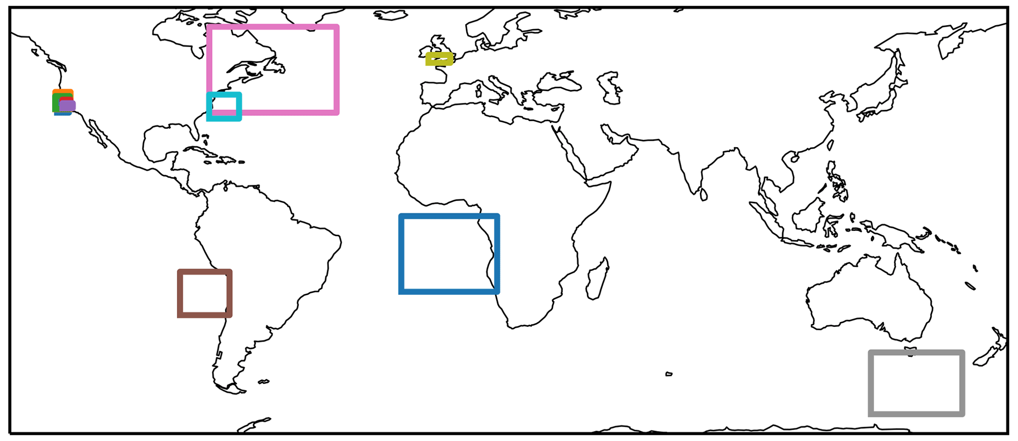
Figure 1 Locations of the campaigns used in this work. Colours are shown in Fig. 2.

Stratocumulus data come from the CIRPAS (Center for Interdisciplinary Remotely Piloted Aircraft Studies) Twin Otter data in Sorooshian et al. (2018), including data from the E-PEACE (Eastern Pacific Emitted Aerosol Cloud Experiment), FASE (Fog and Stratocumulus Evolution Experiment), MACAWS (Marine Aerosol Cloud and Wildfire Study), MASE1 and MASE2 (Marine Stratus/Stratocumulus Experiment) campaigns. These campaigns took place over the northeastern Pacific near the coast (Fig. 1). These campaigns had a consistent use of the CASF (the forward-scattering component of the cloud, aerosol and precipitation spectrometer) and a large number of intersections with the MODIS instrument. For these campaigns the liquid water content (LWC) comes from the PVM-100A probe on the Twin Otter. Data from the NCAR (National Center for Atmospheric Research) C-130 during VOCALS-REx (Variability of the American Monsoon Systems (VAMOS) Ocean-Cloud-Atmosphere-Lands Study – Regional Experiment; Wood et al., 2011) provide measurements of a different stratocumulus region. The C-130 used a cloud droplet probe (CDP) to measure the droplet size spectrum. Data from the phase Doppler interferometer (PDI) on board the P-3 during ORACLES (ObseRvations of Aerosols above CLouds and their intEractionS; Redemann et al., 2021) are used to provide N_d measurements of the Namibian stratocumulus deck. Only data from 2016 and 2018 are used, due to issues with the PDI in 2017.

Four other flight campaigns are used to investigate the N_d retrieval in a broader range of clouds, often in more challenging conditions. Data for North Atlantic boundary layer clouds come from the North Atlantic Aerosol and Marine Ecosystem (NAAMES) campaign (Behrenfeld et al., 2019). A CDP was used to measure the droplet size distribution during a 3-year period (2015–2017). Data from ACTIVATE (Aerosol Cloud meTeorology Interactions oVer the western ATlantic Experiment;  Sorooshian et al., 2019) include N_d data from a CDP during 2020, aimed primarily at shallow liquid clouds (cumulus and winter postfrontal stratocumulus) off the eastern coast of the USA. SOCRATES (Southern Ocean Clouds, Radiation, Aerosol Transport Experimental Study;  McFarquhar et al., 2021), aimed at Southern Ocean clouds, provides CDP observations of N_d in a challenging, often mixed-phase environment. Finally, COPE (Convective Precipitation Experiment Leon et al., 2016) used a CDP to measure N_d in convective environments. For the COPE campaign, LWC data come from the Johnson Williams instrument; for all other campaigns using a CDP, the LWC is calculated from the CDP size distribution.

For each flight campaign, 1 Hz data are used. For the CDP instruments, the total particle number (2–50 µm) is used. For the campaigns using CASF and PDI data, bins are selected (with a linear interpolation for partial bins) to produce an N_d representative of the range 2–30 µm (the exact values have little effect on the results presented in this work). A correction for advection between the satellite and aircraft measurement times is applied, along with a parallax correction based on the aircraft height.

2.4 In situ data sampling

As the aim of this work is to evaluate the satellite sampling strategies and products, extensive filtering on the aircraft data is not performed, relying on the satellite to select cases where there are valid N_d retrievals (as is required for a global product). In particular, no attempt is made to select the N_d value at the cloud top. While the N_d retrieval uses cloud top r_e, it is based on the assumption that N_d is constant throughout the cloud depth. This assumption is valid on average for VOCALS-REx (Painemal and Zuidema, 2011), SOCRATES (Kang et al., 2021) and NAAMES (Painemal et al., 2021) but may not be for a non-adiabatic cloud. A satellite retrieval has to be able to identify these situations.

The LWC–N_d relationship in Fig. 2 shows a very strong relationship at low LWC values, likely due to inhomogeneous mixing reducing N_d and LWC at cloud edges (Baker et al., 1980). To ensure that the in situ N_d measurements are representative of the whole cloud, rather than a mixing region close to a cloud edge, a uniform minimum LWC of 0.1 g m⁻³ is used, discarding aircraft N_d measurements below this when comparing to the satellite retrievals.

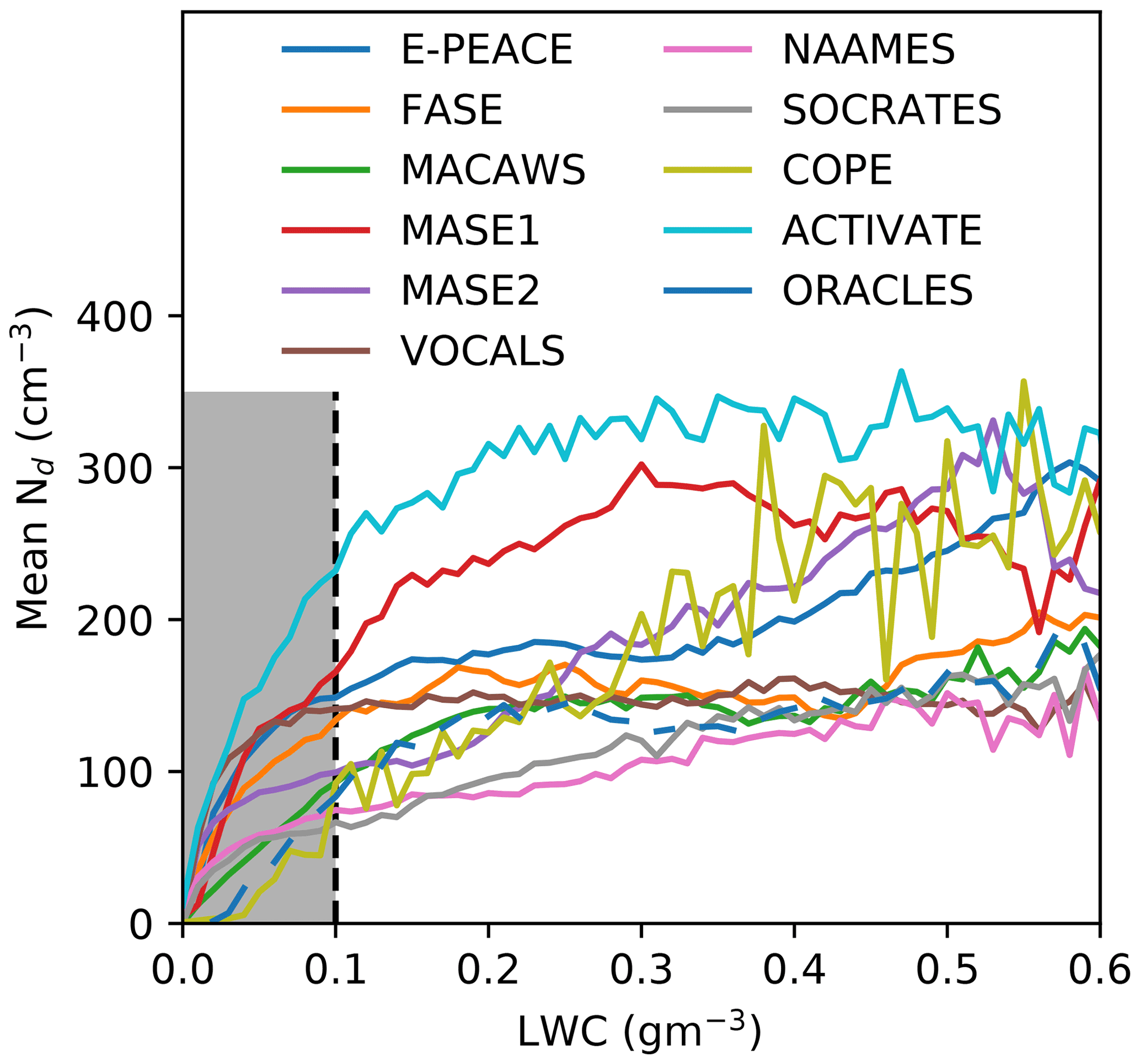
Figure 2 Average aircraft N_d as a function of LWC. Aircraft data with an LWC less than 0.1 g m⁻³ are excluded from this analysis.

The aircraft data are aggregated and compared to MODIS data at a pixel level (1 km × 1 km at nadir). For each MODIS pixel, all the 1 Hz aircraft data within that pixel (that satisfy the sampling criteria) are averaged together. A pixel must have more than two aircraft points (2 s) of data to be included in this analysis. To minimise errors from cloud motion and cloud development, a co-incidence time between the satellite and aircraft data of less than 15 min is required.

2.5 Aerosol data

Assessing the impact of N_d sampling techniques implied radiative forcing from aerosol–cloud interactions (RFaci); the susceptibility of N_d to aerosol (β) variations is calculated (Feingold, 2003):

$$\begin{array}{}\text{(2)}& {\mathit{\beta }}_{N_{\mathrm{d}}}={\displaystyle \frac{\mathrm{d}\ln N_{\mathrm{d}}}{\mathrm{d}\ln A}},\end{array}$$

where A is an aerosol proxy. Three aerosol proxies are used in this work, with all β values calculated at 1^∘ × 1^∘ resolution. The aerosol optical depth (AOD) is a simple proxy used in previous work (e.g. Quaas et al., 2008), but that underestimates the aerosol impact on clouds (Gryspeerdt et al., 2017). The aerosol index (AI), defined as the AOD multiplied by the Ångström exponent (Nakajima et al., 2001), is able to diagnose the RFaci to within 20 %, provided accurate retrievals of AI and N_d (Gryspeerdt et al., 2017). Following Hasekamp et al. (2019), AI retrievals less than 0.1 are discarded due to their high uncertainty. Both AOD and AI are from the daily mean MODIS collection 6.1 1^∘ × 1^∘ product (MYD08_D3). The AOD is the combined Dark Target (Levy et al., 2013) and Deep Blue (Sayer et al., 2014) product, while the AI is calculated from the AOD–Ångström exponent joint histograms over ocean only. Reanalysis aerosol products are also a potential aerosol proxy, correlating well to N_d in a variety of environments (McCoy et al., 2017). The MERRA-2 (Modern-Era Retrospective analysis for Research and Applications) 900 hPa SO₄ concentration is also used as an aerosol proxy, as in McCoy et al. (2017).

To estimate the contribution of sensitivity variations to the implied RFaci, the RFaci is calculated as

$$\begin{array}{}\text{(3)}& \text{RFaci}=F^{\downarrow }{f}_{\mathrm{c}}{\displaystyle \frac{{\mathit{\alpha }}_{\mathrm{c}}\left(\mathrm{1}-{\mathit{\alpha }}_{\mathrm{c}}\right)}{\mathrm{3}}}{\mathit{\beta }}_{N_{\mathrm{d}}}\mathrm{\Delta }\ln A,\end{array}$$

where F^↓ is the CERES downwelling flux; f_c is the MODIS liquid cloud fraction; and α_c is the cloud albedo, derived from the MODIS cloud optical depth. These estimates are calculated at a 1^∘ × 1^∘ resolution.

3 Results

3.1 Satellite and in situ comparison (pixel level)

Given the large number of assumptions and uncertainties in the N_d retrieval, the agreement between MODIS and in situ N_d is surprisingly good (Fig. 3). Coefficients of determination (r² – the square of the Pearson product-moment correlation coefficient) for the stratocumulus campaigns are in the range 0.5 to 0.8 (Table 2). For the more challenging situations, the coefficient of determination is lower (in the range 0.25 to 0.5) but still shows skill at retrieving N_d.

Figure 3 Comparison between MODIS and in situ N_d at a pixel level, for aircraft data within 15 min of a MODIS (Aqua or Terra) overpass. Blue is data that do not satisfy G18; orange dots are G18 sampling; and green are Z18. The instrument used in each campaign and the main cloud type (LSc – liquid stratocumulus) is shown in the top left of each subplot.

Even for the least stringent filtering (All), r² values remain high for the stratocumulus campaigns (as in Painemal and Zuidema, 2011). This agreement holds even for some of the large N_d values (500 cm⁻³) seen in E-PEACE (Fig. 3a) and FASE (Fig. 3b), even though these pixels are removed by the G18 and Z18 sampling strategies as potentially biased.

The retrievals for most of the stratocumulus campaigns have high r² values (Table 2) and close alignment to the 1:1 line (Fig. 3). However, in some of the more challenging situations, particularly NAAMES and SOCRATES, MODIS can overestimate the in situ values (Fig. 3h–k), sometimes by more than 100 cm⁻³. Even the more stringent sampling strategies of G18 and Z18 are unable to identify these pixels as biased, suggesting that further filtering techniques are be required to provide accurate N_d values under these circumstances.

All the sampling strategies fail to accurately characterise N_d from COPE. Convective clouds are a uniquely challenging environment for the N_d retrieval, with strong mixing limiting potential adiabatic locations (Eytan et al., 2021). Not only does this limit the applicability of Eq. (1), but the extremely heterogeneous clouds also limit the accuracy of the MODIS retrievals (Zhang and Platnick, 2011), and large variations in N_d increase representation errors for the aircraft data. The comparisons with ACTIVATE are slightly better, especially for the more restrictive sampling strategies. Even so, MODIS typically produces underestimates of N_d when compared to the in situ data. This is expected in broken-cloud and inhomogeneous scenes, which lead to overestimates in r_e (Zhang and Platnick, 2011) and corresponding underestimates in N_d.

Table 2 Coefficient of determination (r²) for MODIS in situ comparisons for the 2.1 µm retrieval. “–” indicates too few points to calculate a correlation. The “Average” row is the average r² across the campaigns, and the “All” row is the r² value for all the valid data points across all campaigns (with 5 % and 95 % bounds). The bottom rows show the root mean squared deviation (RMSD), the RMSD normalised by the mean N_d and the mean bias (MODIS–in situ) across all the campaigns. Numbers of data points for each campaign are shown in Fig. 6.

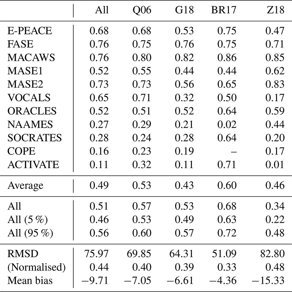
Considering all the available pixel-level matches between MODIS and the in situ data, BR17 produces the strongest overall correlation, with an r² value of 0.68 and a low mean bias (defined as MODIS N_d minus in situ N_d) of −4.36 (Table 2). The bias is negative for all sampling strategies (a MODIS underestimate), likely due to overestimates in the effective radius (Zhang and Platnick, 2011). Both Q06 and G18 are improvements on using all data, with only a 10 % and 25 % reduction in the data volume respectively. In comparison, BR17 discards almost 63 % of available liquid cloud pixels. Interestingly, while Z18 often produces high correlations to the in situ data, the overall r² (0.34) and bias (−15.33) values are lower than any other sampling strategy. This is partly due to it preferentially selecting sub-adiabatic convective retrievals in the more convective campaigns (e.g. COPE), as it selects the highest optical-depth cases. Although the correlation in a single campaign can be high, the bias varies between campaigns and so produces a worse correlation overall.

3.2 Other sampling choices

3.2.1 Should I use a minimum cloud fraction?

The G18 strategy introduces filtering by the 5 km CF, ensuring the retrieval is more than 2 km from a cloud edge. While this reduces the impact of cloud inhomogeneities, some studies have required a high 1^∘ × 1^∘ liquid CF to further reduce the impact of this uncertainty (e.g. Grosvenor et al., 2018a). This can remove broken-cloud scenes where retrieval uncertainties can be higher.

Figure 4 The impact of filtering by (a) large-scale liquid cloud fraction, (b) pixel-level cloud SPI and (c) the maximum permitted r_e on the total r² for each sampling strategy. (d, e, f) As (a), (b) and (c) but for the root mean squared deviation. (f, g, h) As (a), (b) and (c) but for the mean bias.

Specifying a minimum large-scale liquid CF has a relatively small impact on r² (Fig. 4a), with a gradual increase in the total r² as the minimum cloud fraction increases for the majority of sampling strategies. There is a corresponding decrease in the data volume; only around 50 % of investigated pixels have a total liquid CF > 90 %, but it would improve the accuracy of the remaining retrievals if that was the only consideration.

The Z18 sampling shows a slightly larger increase in r² as the minimum CF increases, becoming the highest-accuracy strategy for a high liquid CF (Fig. 4a). This is likely due to the cloud core assumption of Z18 being most valid for closed-cell stratocumulus cases. This suggests that while the Z18 sampling might be less suited to broken-cloud cases, it could be preferred in environments of a high liquid CF.

Similar effects are seen in the RMSD, where there is a small decrease in RMSD as the minimum cloud fraction increases. There is a slight decrease in the mean bias as the minimum liquid cloud fraction increases such that all the sampling strategies have a very similar mean bias for cases of a high liquid CF.

3.2.2 Which SPI threshold should I use?

G18 also introduces a cloud mask SPI threshold, which aims to exclude pixels with sub-pixel variation in cloud properties. Gryspeerdt et al. (2019) used a maximum value of 30 %, finding that further limiting this value made little difference to their results. However, for the pixel-level MODIS–in situ comparison (Fig. 3), limiting the SPI further produces a measurable increase in the accuracy of the MODIS N_d retrieval (Fig. 4b), particularly for the Z18 sampling strategy. This limitation also decreases the RMSD (Fig. 4e) and mean bias (Fig. 4h).

Using a maximum SPI of 5 % reduces the available data with the All strategy by 45 %. This is only a 29 % reduction for the Z18 strategy (where SPI is already limited to a maximum of 30 %; Table 1). If a higher accuracy is required, a lower SPI limit can help achieve this. A very strict SPI limit significantly reduces the accuracy difference between the sampling strategies and may be a more data-efficient way to achieve accuracy levels close to BR17 than r_e stacking (Fig. 4b).

3.2.3 Should I use a maximum r_e?

A large cloud top r_e has been proposed as an indicator of warm rain (Rosenfeld and Gutman, 1994). As a precipitating cloud is non-adiabatic, this creates a systematic bias as a function of r_e. Restricting the N_d calculation to a maximum r_e might potentially increase the overall accuracy of the sampled N_d.

For all the sampling strategies, setting a very low maximum r_e (<15 µm) results in a reduction in the accuracy of the N_d retrieval by removing most of the data being studied (Fig. 4c, f). A very high maximum r_e recovers the values from Table 2. For Z18, there is an increase in accuracy between these two limits, with a maximum correlation between the MODIS and in situ N_d for a maximum r_e of around 15 µm. This may be due to Z18 targeting retrievals in cloud cores where precipitation is more likely. In these situations, removing precipitating cases would have the biggest effect on the accuracy of the N_d retrieval. Further accuracy improvements may be found from using a more sophisticated precipitation threshold, such as H³ / N_d, where H is the cloud depth (vanZanten et al., 2005). In contrast, a maximum r_e has no impact on the BR17 filtering, as the r_e stacking is already designed to filter out precipitating cases.

The impact of a maximum r_e on the mean bias (Fig. 4i) shows some similar properties, with little change at very large values for r_e. For the all data and Z18 strategies, there is a significant improvement in the mean bias limiting retrievals to a maximum r_e of less than 20 µm. This may be related to the focus on cloud cores in Z18 (which are more likely to be precipitating). Very stringent r_e filtering shifts the bias positively for all sampling strategies, due to the reduction in cases of high r_e that produce potential N_d underestimates. However, the exact correction for N_d varies depending on the cloud field, making this an unreliable method for correcting N_d biases.

3.2.4 Which wavelength should I use?

The standard MODIS r_e retrieval uses the 2.1 µm band. In broken-cloud and inhomogeneous conditions, the 3.7 µm r_e retrieval is expected to produce more accurate r_e retrievals (Zhang and Platnick, 2011; Painemal and Zuidema, 2013). For ideal clouds, the 3.7 µm retrieval retrieves r_e closer to the cloud top and the 1.6 µm retrieval deeper into the cloud. With potential compensating errors, it is not clear which wavelength retrieval gives the best N_d.

Table 3 The impact of r_e wavelength on the total r². The second set of values is for only the non-stratocumulus campaigns.

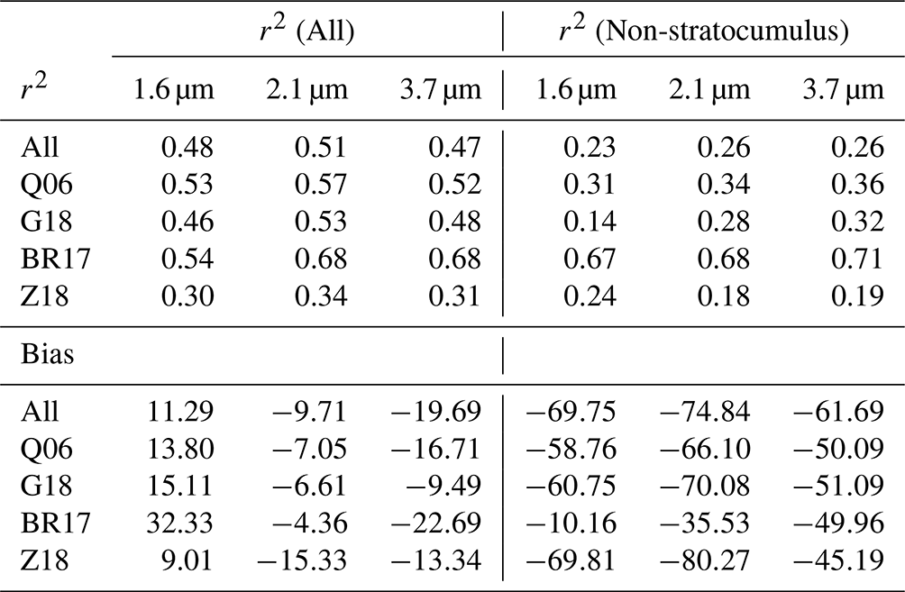
The agreement between the MODIS and in situ N_d values depends on the absorbing wavelength used in the joint τ_c–r_e retrieval (Table 3). When considering all the data together, the 2.1 µm retrieval has a higher r² for all the sampling strategies (with similar performance for the 1.6 µm and 3.7 µm retrievals), other than BR17 (where the effective radius stacking criterion imposes a strict relationship between r_e at different wavelengths). The 2.1 µm retrieval is also the least biased against the in situ data, typically having an underestimate of less than 10 cm⁻³, while the 1.6 µm overestimates N_d, and the 3.7 µm retrieval underestimates N_d by a similar amount.

Considering all the campaigns together hides the behaviour in more challenging situations. In non-stratocumulus situations, the 1.6 µm N_d retrieval does not perform as well as the standard (2.1 µm) retrieval, whereas the 3.7 µm retrieval performs slightly better than the standard (Table 3, right three columns). The variation in non-stratocumulus campaigns is consistent with inhomogeneity generated biases in r_e retrievals, where the 3.7 µm retrieval performs better in broken-cloud environments (Zhang and Platnick, 2011).

The biases in these more challenging conditions are larger and universally negative (due to the r_e overestimate in broken-cloud conditions). The 2.1 µm retrieval shows the largest mean bias under these conditions, with the 3.7 µm retrieval having the smallest bias and the 1.6 µm retrieval being in between. For the BR17 strategy, the 1.6 µm retrieval has the smallest bias, due to the r_e stacking criterion. With a higher r² and a lower mean bias, the 3.7 µm retrieval could be preferred in these broken-cloud conditions.

3.3 Should I correct for penetration depth biases?

The derivation of Eq. (1) assumes r_e is from the cloud top, but satellite retrievals provide r_e at a distance below the cloud top, based on the photon penetration depth (Platnick, 2000). This low bias in r_e is hypothesised to lead to a high bias in N_d, particularly for thin clouds (Grosvenor et al., 2018a).

Applying the Grosvenor et al. (2018a) correction for penetration depth results in a reduced high N_d bias at high N_d for the VOCALS and E-PEACE campaigns (not shown). For the other campaigns, there is either little change or a decrease in N_d retrieval accuracy. This may be due to compensating biases in the N_d retrieval and the Q06 sampling removing cases with low optical depths where this penetration depth bias is strongest. Although this correction is not applied in this work, as the quality of N_d retrievals improves, the penetration depth bias may play a more important role in the overall N_d error budget.

3.4 Satellite and in situ comparison (1^∘ × 1^∘)

Many studies using data derived from the MODIS N_d do so at 1^∘ × 1^∘ resolution. Although in situ data have difficulty representing such a large region, it is instructive to make a simple comparison between MODIS and in situ data at this resolution (see also McCoy et al., 2020). It is not possible to collect aircraft data to perfectly characterise an entire grid box this size. To increase the representation of the data for each grid box, 300 s of in-cloud aircraft data and more than 2000 MODIS pixels are required for each 1^∘ × 1^∘ grid box. Only 200 MODIS pixels are required for the Z18 mask, as it makes an explicit aim to select fewer but more representative MODIS pixels. While there is not an explicit selection for specific campaigns, these representation criteria implicitly bias the results in Fig. 5 towards the liquid stratocumulus campaigns.

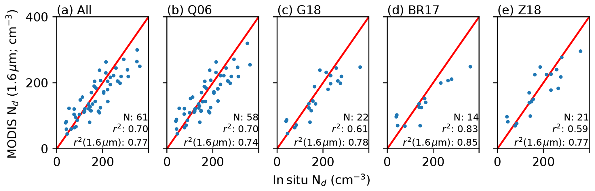
Figure 5 Comparison of 1^∘ × 1^∘ mean in situ and MODIS N_d. Requires at least 300 in situ measurements and 2000 valid MODIS retrievals in a grid box. Each scatterplot also shows the number of points and the r² value, along with the r² value for the 1.6 µm retrieval in the bottom right. The 1.6 µm retrieval is used, as it offers the best correlation to in situ N_d at 1^∘ × 1^∘.

The correlations between the in situ and MODIS data are high (Fig. 5), with r² values above 0.7 even when considering all available liquid pixels. This is considerably higher than the pixel-level correlations in Table 2. The correlations increase for the more restrictive sampling methods, although there is a corresponding decrease in the number of valid grid boxes. The r² value reaches 0.8 for BR17, increasing still further when using the 1.6 µm retrieval (Fig. 5). Although the strategy requiring a large coverage of MODIS and in situ data biases this comparison toward high CF values, stratocumulus regimes where the N_d assumptions are more likely to hold, this comparison gives increasing confidence that the MODIS N_d retrieval is capable of accurately retrieving N_d at a pixel level and over larger regions.

4 Applications

4.1 Representing the N_d climatology

A key requirement for an N_d retrieval is the ability to represent the N_d climatology, especially if it is being used to constrain model simulations (Mulcahy et al., 2018; McCoy et al., 2020). While BR17 has the lowest mean bias (Table 2), this is only for the pixels that satisfy the sampling strategy. This may not be a good representation of the overall N_d climatology. This is already conceptually difficult, as a model maintains N_d even in situations with a very low LWC where a satellite or aircraft is unable to measure N_d, requiring the use of a satellite simulator.

Figure 6 Comparison between the MODIS and in situ N_d distributions for each campaign. In each subplot, the in situ distribution is the left-most boxplot, composed of all the valid in situ data points with a coincident (within 30 min) satellite view (from either Aqua or Terra), independent of whether there is a valid retrieval. Green triangles are the mean, and orange lines are the median. The other boxes in each subplot are the distributions of valid satellite N_d retrievals for each sampling strategy that are coincident with aircraft measurements. The number of N_d data points for each boxplot is given below the x axis; (l) is the average of all campaigns (equally weighted).

Figure 6 shows how well each of the satellite sampling strategies represents the climatology of in situ N_d data for all the potential locations in each campaign. For each sampling strategy, the number of remaining data points is shown along the x axis.

In general, the satellite sampling strategies all do a good job representing the climatology, particularly in stratocumulus regions (as expected following their agreement in this regime; see Fig. 7). However, for NAAMES, both BR17 and Z18 appear to slightly overestimate the mean N_d for the campaign. This may also be the case for ACTIVATE, but the low number of intersections limits our ability to draw strong conclusions. The overestimate in NAAMES appears to be due to the sampling method keeping pixels where MODIS overestimates N_d whilst discarding cases with better agreement but a lower MODIS N_d (Fig. 3g).

The distribution for the complete dataset is dominated by the stratocumulus campaigns, particularly E-PEACE. The similarity of N_d from the different sampling strategies (Fig. 7) means that there is relatively little variation between the regimes, although BR17 and Z18 (and to a lesser extent G18) have a narrower N_d range compared to the in situ data. Weighting each campaign equally (Fig. 6l) shows that, for these campaigns, BR17 has the tendency to remove the lowest N_d values (giving it a slightly high bias) and Z18 tends to remove the highest.

For representing the climatology, this suggests that G18 may be a better choice, particularly outside of stratocumulus regimes. However, the small number of satellite–aircraft comparisons in these cases limits current confidence in the accuracy of the satellite N_d climatology outside stratocumulus.

4.2 Satellite climatologies

The different sampling strategies for the MODIS N_d produce broadly similar N_d climatological patterns (Fig. 7), with higher N_d values over land and in coastal regions and lower values over the remote ocean. While some previous studies have removed data over land, it is kept here, as N_d information over land is used for observation-based estimates of the RFaci.

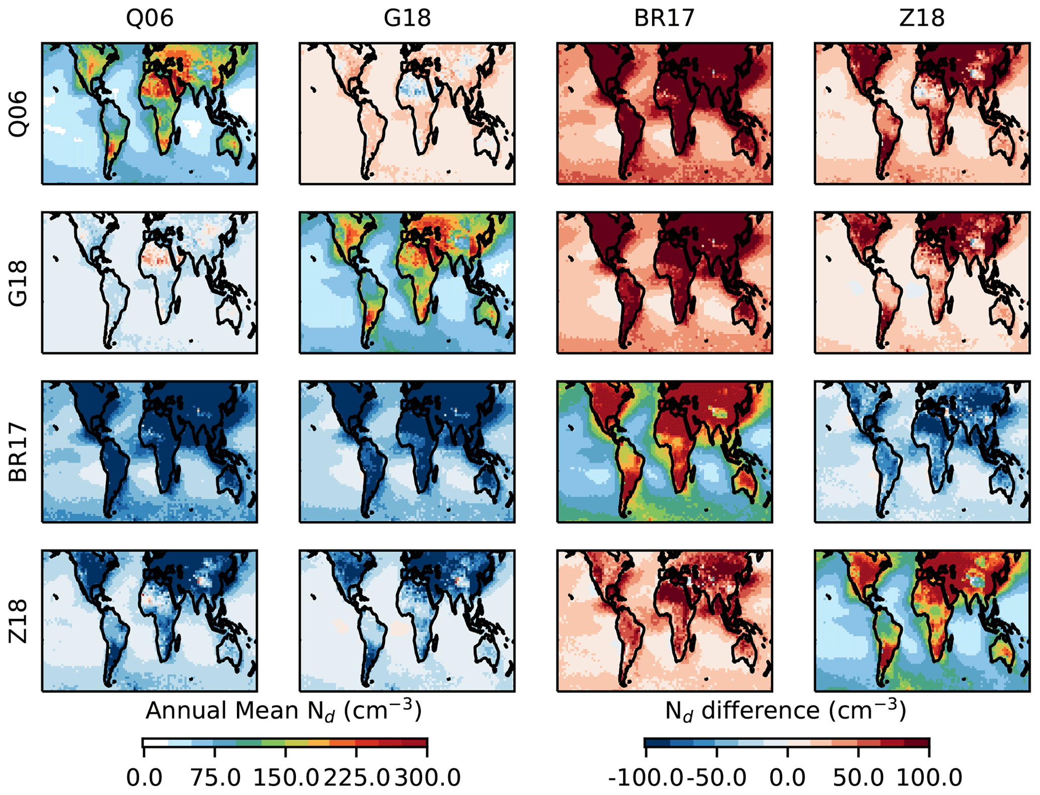
Figure 7 MODIS N_d climatology (2011–2020) for different sampling strategy. The diagonal is the annual mean N_d for each strategy, while the off-diagonal plots show the difference (e.g. the top right is Z18−Q06).

The mean N_d and land ocean contrast differ significantly between sampling methods. While Q06 and G18 have similar global patterns, the G18 mean is typically higher than Q06, with this increase being slightly larger over land than ocean (Fig. 7). BR17 produces a significantly larger N_d across most of the globe (particularly over land) than either Q06 or G18. Similar to BR17, the Z18 enhancement over land is also large (although smaller than BR17), but there is a smaller overall enhancement over ocean.

The difference between the sampling strategies is much smaller in stratocumulus regions, where the CF is larger. In these regions, clouds are much more likely to be adiabatic (and so more likely to satisfy the BR17 r_e stacking criterion). This means that even sampling methods that do not apply this criterion directly will satisfy it most of the time, leading to the small difference in mean N_d between the sampling methods (consistent with the results in Fig. 4a). Over ocean, there is a significant difference in the mean N_d along the eastern coasts of North America and Asia, where the liquid CF is lower and retrievals are more challenging.

4.3 Data coverage

The similarity between the climatologies derived from the different sampling methods hide the very different data coverage (Fig. 8). With a relatively relaxed sampling criterion, Q06 has an N_d retrieval in the majority of available MODIS grid boxes. This is larger than the liquid cloud fraction, as only a single valid N_d pixel is required to count a 1^∘ × 1^∘) grid box as “retrieved”. Only regions with large ice-cloud coverage (the warm pool and over land) have a significantly lower fraction of retrievals.

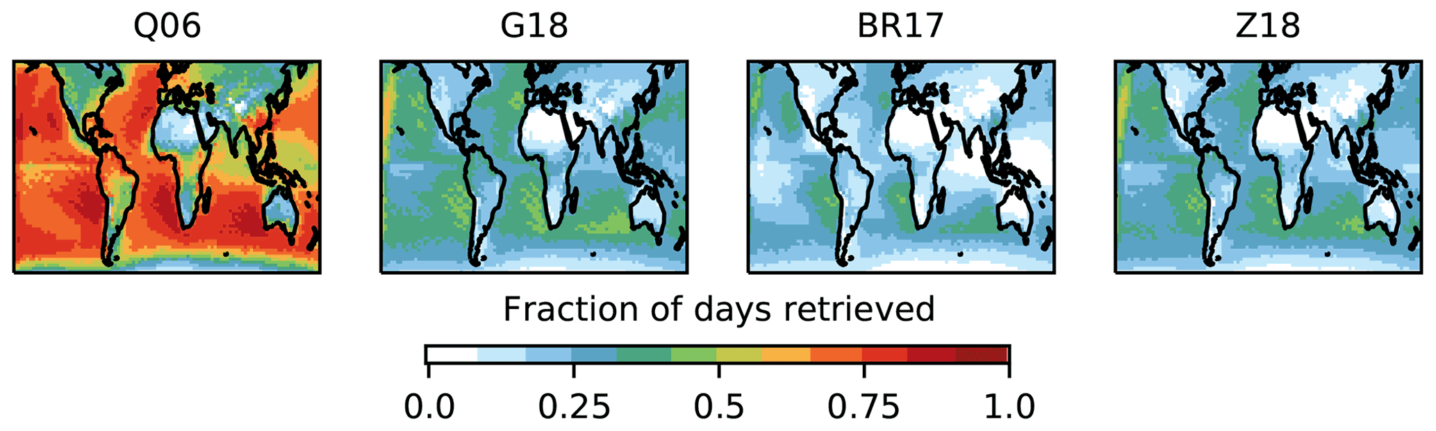
Figure 8 The fraction of 1^∘ × 1^∘ daily pixels with an N_d retrieval for each sampling method.

With much more stringent filtering, G18 provides an N_d retrieval on only around 30 % of days, climbing to around 50 % of days in stratocumulus regions. While many of the G18 sampling conditions are based on geometric properties, these also rely on the cloud SPI, which is typically lower in stratocumulus regions (as they are more homogeneous). This inhomogeneity criterion also contributes to the significantly reduced retrieval fraction over land.

As an even more stringent sampling strategy, BR17 has valid retrievals on an even lower fraction of days. While similar to G18 in the middle of the stratocumulus decks, the requirement for stacked r_e retrievals limits the retrievals primarily to these regions, with very few retrieved points away from stratocumulus decks. Z18 has a pattern similar to G18. As it selects just the highest 10 % of τ_c within each 100 km region, it can return a retrieval on any day in a grid box where G18 has more than 10 valid retrievals, with around 25 % of days having a valid N_d retrieval.

4.4 Aerosol–cloud sensitivities and RFaci

Another major use for N_d is calculating aerosol–cloud sensitivities, either for use as an emergent constraint (Quaas et al., 2009) or for making direct estimates of the RFaci and ERFaci (e.g. Quaas et al., 2008).

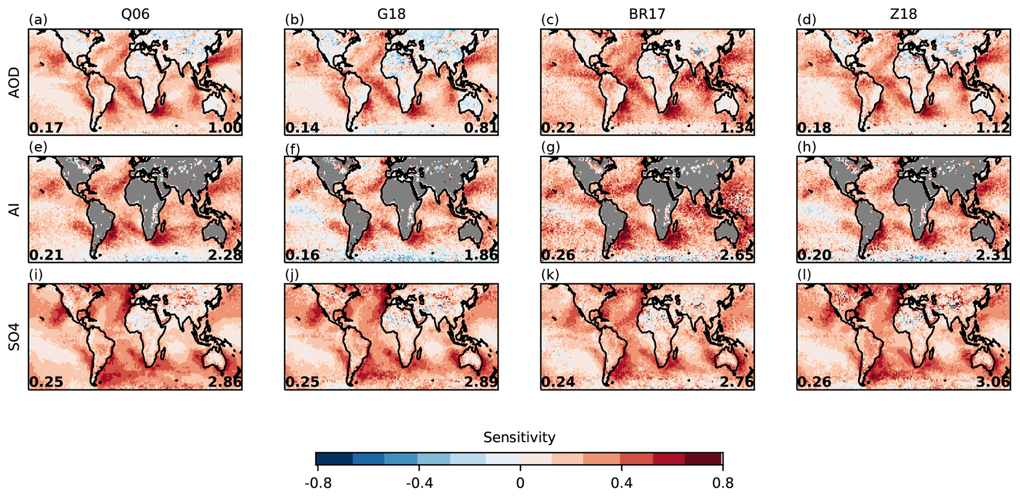
Figure 9 Maps of the sensitivity of N_d to a selection of aerosol proxies (β_N). Each plot shows the global mean β_N in the lower left and the ratio of the implied RFaci to that calculated using Q06 N_d and AOD (a) in the lower right.

As shown in Fig. 9, the sensitivity (as defined in Eq. 2) is largely unaffected by the choice of N_d sampling strategy. The biggest difference appears over land, where BR17 produces a more positive sensitivity when compared to other methods.

The variations in sensitivity and its spatial pattern produce around a 20 % variation in the implied RFaci (Fig. 9, lower-right corners), with larger RFaci values implied when using the BR17 and Z18 strategies. The smaller impact of N_d uncertainties on the RFaci (compared to aerosol uncertainties) is expected, as N_d is the independent variable in the β_N calculation. As such, the correlation between satellite N_d and true N_d does not strongly affect the value of β_N inferred from linear regression for reasonable sample sizes (e.g. larger than a few dozen).

For a simple linear regression calculation, only deviations from a linear relationship between the observed and actual N_d affect the calculated β_N. Biases in N_d that scale with true N_d do not affect inferred β_N because of the power law relationship assumed in the regression. Examining the correspondence between aircraft N_d and satellite N_d in Figs. 3 and 5 supports a linear relationship with zero intercept, even in cases where they do not fall along the 1:1 line. Thus the N_d calculation methods examined here appear to be all be of sufficient accuracy to produce accurate estimates of β_N. However, bi-variate methods for calculating β_N (e.g. Pitkänen et al., 2016) are more sensitive to the estimates of uncertainty in the N_d retrieval and would have a different error profile. In addition, as N_d is the independent variable in many calculations of cloud adjustments, the uncertainty here still has a critical role to play in the calculation of the ERFaci.

Figure 9 demonstrates that although the aerosol proxy is still the major source of uncertainty in observation-based estimates of the RFaci and ERFaci, the N_d sampling strategy is a non-negligible source of uncertainty because it affects the aerosol proxy data considered and thus sampled deviations between aerosol proxy and actual CCN. It is not clear which of these sampling strategies provides the best estimate of the RFaci. Although BR17 is the most accurate at a pixel level (Table 2), it is based on a subset of cases which may not be representative of the overall climatology (Fig. 6). Further studies will be necessary to understand the impact of this potential selection bias.

5 Discussion and conclusions

N_d is an important property of clouds, both for assessing cloud models and for constraining aerosol–cloud interactions. However, its retrieval is based on a number of assumptions of varying validity. In addition, it is derived from retrievals of τ_c and r_e (Eq. 1) that are themselves uncertain, inheriting potential biases from these retrievals. In recent years, a number of sampling strategies have been suggested (Table 1) to select cases where the assumptions are more likely to be valid and the retrievals less likely to be biased. This work investigates these assumptions and their impact on the implied radiative forcing.

At a pixel level (1 km), the satellite N_d (from MODIS) and in situ N_d are well correlated (Fig. 3). This is especially true in stratocumulus regimes (r² in the range 0.5 to 0.8, Table 2), where high-cloud fractions and adiabatic clouds are more common. Even in more challenging cumulus and convective situations, the MODIS N_d retrieval can provide useful information about N_d, although correlations are significantly lower. These correlations are lower than previous studies (Painemal and Zuidema, 2011; Kang et al., 2021), but the demands placed on the retrieval in this work are much tougher, requiring the satellite sampling strategy to identify accurate retrievals, with no additional data from in situ measurements.

The different sampling strategies have varying strengths and weaknesses. BR17 has the strongest correlation to in situ N_d across a range of aircraft campaigns but has the lowest coverage of any of the strategies investigated (Fig. 8). While Z18 has a lower accuracy than other strategies, it has a higher correlation to in situ N_d in locations of a high CF. It is important to note that the BR17 and Z18 strategies in this work are applied on top of G18 (Table 1), differing from their original application in Bennartz and Rausch (2017) and Zhu et al. (2018). BR17 and Z18 both benefit from the identification of uncertain retrievals provided by G18.

The RMSD, normalised by the mean N_d for each of the sampling strategies, is around 30 %–50 % (Table 2). This is significantly smaller than the 78 % uncertainty calculated in Grosvenor et al. (2018b), partly due to the focus more on stratocumulus cases in this work and partly due to the success of the sampling strategies in identifying and excluding biased N_d retrievals.

Potential improvements to the sampling strategies are demonstrated (Fig. 4), leading to a number of recommendations for the use of MODIS-derived N_d products in the future.

• A high correlation between MODIS and in situ N_d is achieved even with minimal filtering. This can represent the variability in N_d better than the more selective sampling methods (Fig. 6).

• BR17 appears to have the best correlation with aircraft data across a wide variety of conditions (Table 2) but may be biased high in broken-cloud conditions (Fig. 6).

• Z18 has a lower skill for low-cloud fractions, but the accuracy increases for high-cloud fractions (likely due to the validity of the assumptions used; Fig. 4).

• The 3.7 µm retrieval is a better match to in situ data in non-stratocumulus cases, consistent with studies looking at the effective radius retrieval. There may be a small advantage to using the 1.6 µm retrieval for 1^∘ × 1^∘ averages (Fig. 5). This may be due to cloud top entrainment effects, but given the known uncertainties in the 1.6 µm r_e retrieval (Zhang and Platnick, 2011), confidence in this result is low, and users should be cautious if they intend to employ the 1.6 µm N_d retrieval.

• Across the campaigns, G18 has the closest match to the climatology (Fig. 6). However, the difference between sampling strategies in stratocumulus regions is small, and the lack of satellite–in situ coincidences in non-stratocumulus regimes reduces confidence in this result in these locations.

The correlation between in situ and satellite N_d increases further when considering 1^∘ × 1^∘ averages, with r² values of almost 0.9 for the BR17 sampling strategy (Fig. 5). However, the uncertainty in these correlations remains high due to the small number of data points and the high representation errors for aircraft measurements of a 1^∘ × 1^∘ region.

Even with the different climatologies produced by the sampling strategies (Fig. 7), the susceptibility of N_d to aerosol proxies remains remarkably similar (Fig. 9). The similarity is closest in stratocumulus regions, resulting in N_d sampling generating only a 20 % variation in the implied forcing. The impact of the aerosol proxy on the estimated RFaci remains the largest uncertainty, although N_d sampling produces an uncertainty of around 20 %.

The apparent close agreement between MODIS and in situ N_d masks a number of uncertainties. While N_d measurements in stratocumulus regions agree well, there is significant diversity in the N_d estimates in non-stratocumulus cases. While these are less important for the RFaci (Gryspeerdt and Stier, 2012), they may be critical for the forcing from cloud adjustments (e.g. Koren et al., 2014), and observations of N_d in these regions are essential for constraining the magnitude of these adjustments (Gryspeerdt et al., 2016). Additionally, biases in N_d may be correlated to biases in other cloud properties (such as the LWP). Understanding and reducing these systematic biases is beyond the scope of this work but vital to make progress in observationally constraining aerosol–cloud interactions.

While significant uncertainties remain, this work has demonstrated that the MODIS N_d retrieval has skill in retrieving N_d in a variety of different cloud regimes. There is a close match between not only in situ and satellite data at a pixel level but also the in situ and satellite N_d climatologies, with a sufficient accuracy for addressing a wide range of questions in cloud and aerosol–cloud physics at the global scale.