the Creative Commons Attribution 4.0 License.
the Creative Commons Attribution 4.0 License.
 | 07 Jul 2022
Testing the efficacy of atmospheric boundary layer height detection algorithms using uncrewed aircraft system data from MOSAiC
John Cassano
Sandro Dahlke
Gijs de Boer
During the Multidisciplinary drifting Observatory for the Study of Arctic Climate (MOSAiC) expedition, meteorological conditions over the lowest 1 km of the atmosphere were sampled with the DataHawk2 (DH2) fixed-wing uncrewed aircraft system (UAS). These in situ observations of the central Arctic atmosphere are some of the most extensive to date and provide unique insight into the atmospheric boundary layer (ABL) structure. The ABL is an important component of the Arctic climate, as it can be closely coupled to cloud properties, surface fluxes, and the atmospheric radiation budget. The high temporal resolution of the UAS observations allows us to manually identify the ABL height (ZABL) for 65 out of the total 89 flights conducted over the central Arctic Ocean between 23 March and 26 July 2020 by visually analyzing profiles of virtual potential temperature, humidity, and bulk Richardson number. Comparing this subjective ZABL with ZABL identified by various previously published automated objective methods allows us to determine which objective methods are most successful at accurately identifying ZABL in the central Arctic environment and how the success of the methods differs based on stability regime. The objective methods we use are the Liu–Liang, Heffter, virtual potential temperature gradient maximum, and bulk Richardson number methods. In the process of testing these objective methods on the DH2 data, numerical thresholds were adapted to work best for the UAS-based sampling. To determine if conclusions are robust across different measurement platforms, the subjective and objective ZABL determination processes were repeated using the radiosonde profile closest in time to each DH2 flight. For both the DH2 and radiosonde data, it is determined that the bulk Richardson number method is the most successful at identifying ZABL, while the Liu–Liang method is least successful. The results of this study are expected to be beneficial for upcoming observational and modeling efforts regarding the central Arctic ABL.
- Article
(8076 KB) - Full-text XML
-
Supplement
(4957 KB) - BibTeX
- EndNote


The transfer of energy between the Earth's surface and the overlying atmosphere, particularly at high latitudes, remains an area of substantial uncertainty in our understanding of the global climate system (de Boer et al., 2012; Tjernström et al., 2012; Karlsson and Svensson, 2013). The consequences of this uncertainty are significant, with global climate model projections of present-day sea ice demonstrated to fall short of simulating the observed rate of change (Stroeve et al., 2007, 2012). The thermodynamic structure of the lower atmosphere plays a central role in regulating cloud life cycle and radiative transfer, and their influence on atmospheric energy transport (Tjernström et al., 2004; Karlsson and Svensson, 2013; Brooks et al., 2017). Significant insight can be gained by measurements collected over the central Arctic Ocean pack ice, focused on the structure of the lower atmosphere, its spatial and temporal variability, the intensity of turbulent energy fluxes, and its connection to surface features. To provide such measurements, uncrewed aircraft were deployed in the lower atmosphere during legs 3 (March through May 2020) and 4 (June through August 2020) of MOSAiC (Multidisciplinary drifting Observatory for the Study of Arctic Climate; Shupe et al. 2020), a year-long expedition that took place from October 2019 to September 2020 in which the icebreaker RV Polarstern (Alfred-Wegener-Institut Helmholtz-Zentrum für Polar- und Meeresforschung, 2017) was frozen into the central Arctic Ocean sea ice pack and allowed to passively drift across the central Arctic for an entire year (Fig. 1). Additional information on measurements taken of the atmosphere and sea ice during MOSAiC can be found at Shupe et al. (2022) and Nicolaus et al. (2022), respectively.
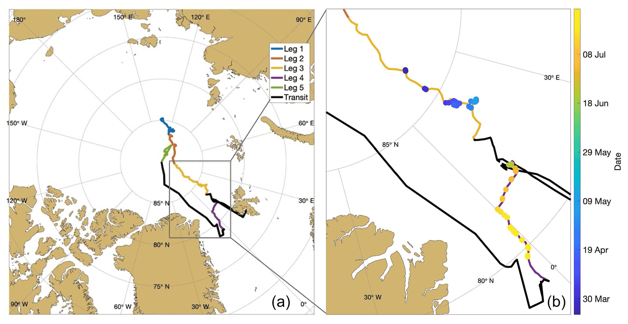
Figure 1(a) The drift track of the Polarstern, separated by color into the five different legs. The black “transit” line indicates when the ship was traveling under its own power between legs 3 and 4 and between legs 4 and 5. (b) The zoomed-in portion of the Polarstern drift during which DH2 flights were conducted (legs 3 and 4). The locations of all of the DH2 flights are overlaid on the drift track and color coded by date: blue-tinted dots indicate flights conducted during leg 3, and yellow-tinted dots indicate flights conducted during leg 4.
One important indicator of the extent to which energy may be transferred between the Earth's surface and overlying atmosphere is the atmospheric boundary layer (ABL) height. The ABL is the turbulent lowest part of the atmosphere that is directly influenced by the Earth's surface (Stull, 1988; Marsik et al., 1995). In the central Arctic, the ABL is impacted by interactions between the atmosphere and underlying surface, including both sea ice and open-water portions, which can cause either buoyantly or mechanically produced turbulence. The generation of buoyant turbulence can occur through surface energy fluxes emitted from open water regions such as leads (Lüpkes et al., 2008), cold air advection, especially over thin ice (Vihma et al., 2005), or turbulent mixing below cloud base due to cloud top radiative cooling (Tjernström et al., 2004). Mechanical generation, which is the dominant driver of turbulence in the central Arctic (Brooks et al., 2017), can occur due to the interaction between the atmosphere and surface roughness features such as ridges and ice edges (Andreas et al., 2010) or oceanic waves (Jenkins et al., 2012) or due to the presence of a low-level jet (Brooks et al., 2017; Banta et al., 2003). Solar heating of the Earth's surface and the subsequent formation of buoyant thermals, which is a dominant forcing of the ABL in most parts of the planet (Marsik et al., 1995), plays only a minor role in the central Arctic due to the relatively reflective surfaces found there.
The Arctic ABL is usually either stable or near neutral, while a convective ABL is rarely observed (Brooks et al., 2017; Esau and Sorokina, 2010). A stable boundary layer forms when there is a deficit of radiation at the surface or when warmer air is advected over a cooler surface and can range from being nearly well mixed with moderate turbulence to nearly laminar (Stull, 1988). A neutral boundary layer occurs when air at the surface is neutrally buoyant (Sivaraman et al., 2013); this is primarily due to mechanically generated turbulence that mixes air between the surface and the above atmosphere (Brooks et al., 2017). A convective boundary layer forms when convective thermals create positive buoyancy (Liu and Liang, 2010) and an air parcel at the surface rises adiabatically until becoming neutrally buoyant; when this phenomenon occurs in the central Arctic, it is likely due to the presence of open water such as leads or polynyas (Lüpkes et al., 2008). While the various forms that the Arctic ABL may take are complex, most of the time the Arctic ABL is capped by a temperature inversion (which may extend to the surface for a stable ABL) and the local maximum in the potential temperature gradient, marking the entrainment zone, which is a stable layer that makes the transition from the ABL to the free atmosphere (Stull, 1988). One important difference between the Arctic ABL and that in the mid-latitudes is that there is usually no residual layer above a stable Arctic ABL due to the lack of a diurnal cycle. Additionally, the Arctic ABL is typically much shallower than that at mid-latitudes (Esau and Sorokina, 2010). These discrepancies cause certain ABL height detection methods to fail when applied to Arctic data.
Knowing the height of the Arctic ABL is important for many applications. First, it is a metric that represents the altitude up to which the atmosphere is directly impacted by surface processes. This can then inform the extent to which the surface interacts with atmospheric features such as clouds (and their influence on radiative transfer in the lower atmosphere), low-level jets (LLJs), and temperature inversion layers, which all have important implications for Arctic warming (Serreze and Barry, 2011). For example, a shallow, stable ABL is more likely to be observed with clear skies above (Brooks et al., 2017), which promotes longwave cooling of the surface and decoupling from the above atmosphere. In this instance, a surface-based temperature inversion is likely to constrain warming to the surface, which contributes to Arctic amplification (Lesins et al., 2012). ABL height (hereafter ZABL) plays an important role in many other applications, including transfer of air pollutants and weather forecasting (Garratt, 1994), and the proper parameterization of the ABL in numerical weather prediction models. Since any determination of ZABL is simply an approximation, the most value can be gained if this approximation is as accurate as possible. The goal of the current work is to determine which methods, based on thermodynamic and kinematic uncrewed aircraft system (UAS) profile data, can best accomplish this.
Table 1List of quantities previously used to identify ZABL, as well as some associated literature in which each variable is referenced.
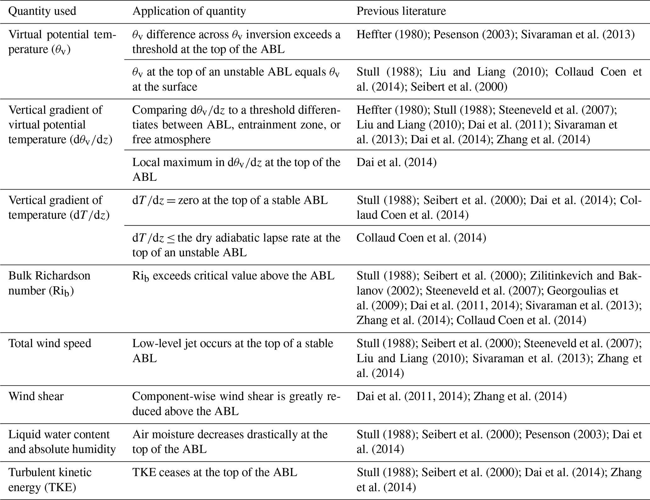
The depth of the ABL has been previously defined using a variety of approaches that involve visualizing the profiles of different thermodynamic and kinematic variables, which are listed in Table 1, along with some examples of associated literature that references use of that variable. Each of these profiles typically exhibits a distinct change in vertical structure at the top of the ABL. Additional methods may exist, such as analyzing the vertical gradient of aerosol content, but are not listed since the current study focuses on ZABL determination using thermodynamic and kinematic processes.
Due to the different atmospheric dynamics involved in each of the above approaches, the definition of ZABL is often debatable amongst experts. Depending on one's purpose for knowing ZABL, different approaches may be most applicable. Of these methods, some of the most widely used ones and the ones applied in the current analysis of a central Arctic dataset to determine ZABL are the ones that involve analysis of virtual potential temperature (θv), vertical gradient of virtual potential temperature (), humidity (relative and absolute), bulk Richardson number (Rib), and wind speed profiles. The current focus is on these variables because the physical basis for each one as an indication of ZABL is relevant for the Arctic atmosphere. Specifically, θv helps identify the entrainment zone above the ABL, the vertical gradient of humidity either decreases or increases noticeably above the ABL (Dai et al., 2014), Rib helps identify where turbulence (usually caused by strong wind shear or surface roughness in the Arctic ABL; Grachev et al., 2005) ceases above the ABL, and wind speed helps identify the top of the ABL when it is capped by an LLJ, as the ABL top is often at or just below the LLJ core (Stull, 1988). Other methods, such as that using temperature inversion top to identify ZABL (Collaud Coen et al., 2014), do not perform well in the Arctic where a weak temperature inversion can extend well above the ABL. Though turbulent kinetic energy is recognized as perhaps the most valuable profile for ZABL identification (Stull, 1988; Seibert et al., 2000; Dai et al., 2014; Zhang et al., 2014), these data are not available to aid in the current study.
High-resolution data collected by the DataHawk2 UAS allow for determination of ZABL with high accuracy through manual visual analysis. However, visually determining ZABL case by case is time consuming for processing a large dataset. Therefore, the UAS-derived dataset is leveraged to compare manually (or “subjectively”) determined ZABL with that identified through previously published automated (or “objective”) methods. While this subjective ZABL may not necessarily be the “true” ABL top, as the definition of this quantity can be debatable among experts and ZABL is not constant over time, it is the best estimate of ZABL given the available data. This evaluation is completed to identify objective methods that can accurately diagnose ZABL across a larger dataset of central Arctic atmospheric conditions.
To subjectively identify ZABL in each atmospheric profile from DH2 data, the stability regime of the ABL (stable, neutral, or convective) is categorized and ZABL is visually identified through combined evaluation of θv, humidity (both relative humidity, RH, and mixing ratio), and Rib profiles. Objective identification of ZABL is derived through the application of four previously published methods: the Liu–Liang method (Liu and Liang, 2010), the Heffter method (Heffter, 1980), the virtual potential temperature gradient maximum (TGRDM) method (Dai et al., 2014), and the Rib method (Sivaraman et al., 2013), all adapted to best suit the DH2 profiles examined (aside from the Heffter method, which was kept as standard). Following this, statistical comparisons between the objective and subjective ZABL are conducted. Next, the objective methods are applied in their adapted form to radiosonde profiles nearest in time to each DH2 flight to determine if these methods are robust across different measurement platforms for central Arctic conditions. Finally, discussion is included about the features that do or do not lend themselves to accurate identification of ZABL by the objective methods, and findings are summarized to support future studies seeking to identify ZABL quickly, objectively, and accurately across large atmospheric datasets collected in the central Arctic.
2.1 The DataHawk2
Data presented in this study were obtained between 23 March and 26 July 2020 using the University of Colorado DataHawk2 (DH2) UAS (de Boer et al., 2022). Flights were conducted from the sea ice alongside the Polarstern, known as the MOSAiC floe, ranging in location from 86.2∘ N, 15.8∘ E on 23 March, to 79.8∘ N, 1.9∘ W on 26 July 2020 (Fig. 1). Throughout this period, the MOSAiC floe evolved from snow-covered rigid ice situated in the high Arctic to being covered with melt ponds and leads close to the sea ice edge. The surface atmospheric temperatures also transitioned from nearly −35 ∘C at the beginning of leg 3 to hovering near 0 ∘C throughout the entirety of leg 4.
The DH2 (Hamilton et al., 2022) is a fixed-wing, battery-powered UAS (1.1 m wingspan, 1.8 kg weight, 40 min endurance) carrying various meteorological sensors, which measure the state of the atmosphere in Earth-relative coordinates. Instrumentation includes a fine wire array providing high-frequency (800 Hz) information on temperature and air speed, multiple sensors for temperature and relative humidity (Vaisala RSS421 measuring at 5 Hz and SHT-85 measuring at 100 Hz), and upward and downward looking thermopile sensors to provide infrared brightness temperatures of the sky and surface. Air pressure is measured at 5 Hz by the Vaisala RSS421 sensor. Altitude estimates are obtained using a global navigation satellite system (GNSS) receiver and barometer onboard. The altitude used in the current analysis is a high-resolution (800 Hz) barometric pressure altitude, which is corrected for drift using the GNSS altitude.
Measurements of attitude from the inertial measurement unit, airspeed from a Pitot static probe, and ground speed from the GPS receiver support the derivation of high-frequency (10 Hz) horizontal wind estimates. First, the “standard” approach, as laid out in van den Kroonenberg et al. (2008) and Hamilton et al. (2022), is applied, which derives wind estimates by combining GPS velocity measurements in the wind triangle using attitude estimates to rotate airframe-relative winds to Earth-relative coordinates. Additionally, a “hybrid” approach, as laid out in Lawrence and Balsley (2013) and Hamilton et al. (2022), is applied, which derives wind estimates by primarily using airspeed magnitude and GPS velocity, with secondary use of attitude estimates. For the purposes of this study, we use the DH2 winds derived from the “hybrid” approach. Please see Hamilton et al. (2022) and de Boer et al. (2022) for additional details on the wind derivation as specifically applied to the DH2. In addition, because take-offs and landings were flown manually by a remote pilot, the winds calculated during these times were found to be less reliable and accurate. As a result, we do not use DH2 winds calculated below 30 m altitude for this study. A brief description of the processing methods for the above variables are provided in the metadata for the DH2 dataset used for the current study (Jozef et al., 2021).
Table 2Accuracy and reliability of the variables recorded by the Vaisala RSS421 sensors used in this study.
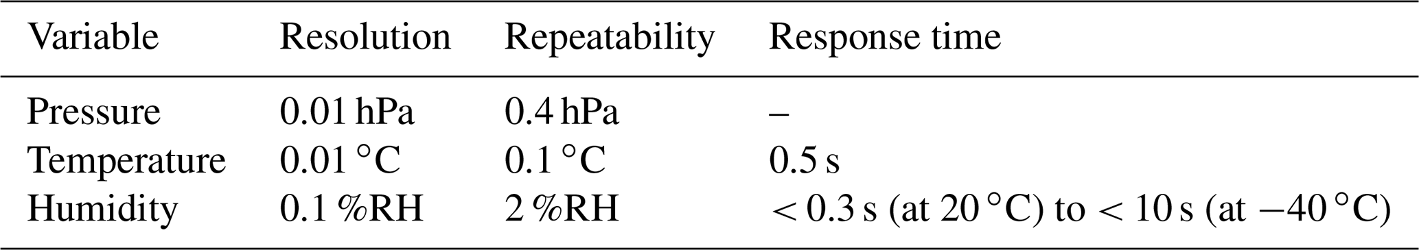
Combined, these sensors provide a comprehensive picture of atmospheric thermodynamic and kinematic state along with some context on the surface and sky condition under which these measurements were obtained. Table 2 lists the resolution, repeatability (standard deviation of difference between two successive repeated calibrations), and response time for the Vaisala RSS421 sensor. Uncertainty in the wind speed estimation is not provided, as determining this is still in progress.
Measurements collected by the DH2 are logged at different frequencies, requiring the implementation of a time alignment process to assure that the time index for each data point of each variable is consistent with all other measurements. Data collected by the DH2 during MOSAiC are available for public download through the National Science Foundation Arctic Data Center at https://doi.org/10.18739/A2KH0F08V (Jozef et al., 2021).
During MOSAiC, DH2 flights were conducted whenever flight weather criteria were met and when the team was able to access the ice alongside the Polarstern. The weather criteria include near-surface wind speeds with a sustained average below 10 m s−1 and gusts below 14 m s−1, as well as sufficient visibility to maintain visual contact with the aircraft at all times during flight. In addition, DH2 flights required coordination with other MOSAiC activities, especially those impacting air space over the MOSAiC floe, including manned helicopter flights and other UAS and tethersonde operations.
The most common flight pattern conducted with the DH2, and the flight pattern from which data for this analysis was acquired, was a profiling flight in which the plane flew a spiral ascent and descent pattern, with a radius of 75–100 m between the surface and 1 km altitude (or cloud base, if lower than 1 km), with the aircraft ascending and descending at a rate of 2 m s−1 and flying at an airspeed of 14–18 m s−1. Each profiling flight lasted an average of 30 min, with some shorter flights when the air temperature was at its coldest (∼ −35 ∘C) near the beginning of leg 3 and some longer flights when the air temperature was much warmer (∼ 0 ∘C) during leg 4. Throughout the measurement period, 89 flights were conducted with the DH2. In the present study, 65 of these flights are found to have a clearly identifiable ZABL within the altitude range sampled. The remaining flights sampled only the lowest portion of the atmosphere due to cloud cover or other unfavorable environmental conditions and therefore did not observe the full depth of the ABL.
2.1.1 Preparing the DataHawk2 data for analysis
The primary profiles of interest for subjective and objective ZABL identification are θv, humidity (RH and mixing ratio), wind speed, Rib, and . θv was calculated using RSS421 temperature, pressure, and RH. Differences in response times of the RSS421 temperature and RH sensors has a negligible impact on the calculation of θv because the moisture content in the Arctic atmosphere is so low that θ and θv values typically differ on the order of less than 1 K. Regardless, the addition of humidity does not change the structure and location of features in the θv profile, which is what is important for ZABL identification. To further eliminate the effects of differences in sensor response times during ascent and descent and for ease of visualization, we average the θv, humidity, and wind speed variables over 1 m altitude bins throughout the entire flight (e.g., values at 10.5 m are averaged from 10 to 11 m). This also mitigates the effect of changes in atmospheric conditions near the surface throughout the span of a flight, although the near-surface observations largely remained constant during a given flight. A value of 1 m is chosen as an averaging bin because using a greater bin value would eliminate much of the fine-scale detail in the θv and humidity profiles which the DH2 provides and which makes its data a valuable resource in honing ZABL detection methods. However, since fine-scale fluctuations in wind speeds evident at the 1 m scale are usually artifacts of the wind estimation routines applied to a circular flight pattern, we additionally apply a 60 m running mean, which eliminates small-scale wiggles while retaining the important large-scale features. Next, we exclude periods of manual flight during takeoff and landing (this is usually at altitudes below 5 m) since measurements during manual flight are prone to inaccuracies due to the irregular flight pattern. Lastly, we exclude the first 5 s of flight, as the initial measurements after takeoff may be faulty due to hysteresis associated with the sensor sitting still at the surface before launch.
Using the 1 m averaged θv and wind speed component profiles, we calculate the Rib profile. Rib is calculated at altitude, z, using the following equation from Stull (1988):
where g is acceleration due to gravity, is mean virtual potential temperature over the altitude range being considered, z is altitude, u is zonal wind, v is meridional wind, and Δ represents the difference over the altitude range used to calculate Rib throughout the profile. The only way that Rib can be negative is if the value for Δθv is negative, indicating a convective atmosphere with buoyancy-driven generation of the turbulence. Rib profiles are created by calculating Rib over a 30 m altitude range (Δz), at 5 m resolution (i.e., between 30 and 60 m, then between 35 and 65 m, and so on), rather than using the ground as the reference level, in order to isolate local likelihood of turbulence rather than that over the full depth from the surface (Stull, 1988; Georgoulias et al., 2009; Dai et al., 2014).
Since we do not use DH2 winds below 30 m, an intermediate Rib value between the surface and 30 m is calculated using an assumed zero wind at the surface. This results in Rib values at 15, 45, 50, 55 m, and so on. It is not crucial to consider the drift speed of the ice for the calculation of this initial Rib value since the ice drift speed during MOSAiC was on average less than 0.1 m s−1 (Krumpen et al., 2021), and the maximum drift speed during the DH2 flights was about 0.3 m s−1, which is negligible compared to the speed of the observed winds. Nevertheless, any error in Rib that ensues due to the drift speed of the ice is limited to the first level where Rib is determined. Lastly, the profile is similarly created by calculating it over an altitude range of 30 m, at 5 m resolution.
The above profiles are used to determine stability regime, visually identify ZABL using criteria found in this paper, and objectively identify ZABL using the four published methods. For the remainder of this paper, ZABL determined from manual visual identification is referred to as the “subjective” ZABL and that determined by the published methods (which are automated algorithms performed by computers) are referred to as “objective” ZABL. These terms are used as a simplification to differentiate between manual and automated methods, though they both consider much of the same underlying physical processes that dictate ABL structure and height.
2.2 Determining the stability regime
Some of the methods for both subjectively and objectively identifying ZABL differ depending on the stability regime, and thus the sampled regime is first identified for each DH2 flight. The three possible stability regimes considered include a convective boundary layer (CBL), stable boundary layer (SBL), and neutral boundary layer (NBL; Liu and Liang, 2010). In a CBL, θv near the surface is greater than that of the overlying ABL (Stull, 1988). In an SBL, the vertical gradient of θv is positive (Stull, 1988). In an NBL, θv at the surface is approximately the same value as that of the overlying remainder of the ABL (Stull, 1988).
Therefore, stability regimes are identified by comparing θv between the lowest altitude sampled by the DH2 (“i” in the below equations; typically ∼ 5 m since altitudes below this are usually sampled with manual flight) and 40 m above, using Eqs. (2)–(4) below, which are adapted from Liu and Liang (2010).
In these equations, δs is a stability threshold that represents the minimum positive or negative vertical difference of θv near the surface necessary for the ABL to qualify as an SBL or CBL, respectively. If this minimum is not either negatively (in the case of a CBL) or positively (in the case of an SBL) reached, the ABL is identified as an NBL (Liu and Liang, 2010). In an idealized case, δs would be zero. However, in practice it must be specified as a small positive number, and this number depends on the surface characteristics as well as inherent uncertainties or noise in the measurements. For profiles over ocean and ice, this threshold has been defined to be 0.2 K (Liu and Liang, 2010).
While Liu and Liang (2010) compare θv between pressure levels that equate to approximately 40 and 160 m in the conditions we sampled, this range was found to be inadequate for differentiating between an SBL, NBL or CBL in the Arctic, where the top of the ABL is often below 160 m, and sometimes even below 40 m. Therefore, considering the θv change below ∼ 45 m more accurately reflects the stability regime of the Arctic ABL. Once the stability regime is identified, criteria based on the θv, humidity, and Rib profiles are applied to subjectively determine ZABL. For the current dataset, 31 SBL cases, 32 NBL cases, and 2 CBL cases were identified.
2.3 Subjective identification of atmospheric boundary layer height
There is no one best method for subjectively identifying ZABL that is agreed upon throughout the scientific community, evident by the many methods outlined in Table 1, and therefore a subjectively determined ZABL is prone to error. The best we can do to increase the confidence in a subjectively determined ZABL is to take into account several of the most commonly used methods and establish criteria which are applied consistently across all profiles. We describe these criteria below.
To subjectively identify ZABL, the θv profile is first analyzed, as the θv profile changes structure above the ABL (Stull, 1988). For a CBL and NBL, above the ABL, θv changes from decreasing or constant with height to increasing with height, marking the entrainment zone (Stull, 1988). The structure of an SBL, however, can vary a lot more (Mayer et al., 2012; Steeneveld et al., 2007; Zilitinkevich and Baklanov, 2002). In an ideal SBL case, the θv inversion is at its strongest (greatest vertical gradient of θv) near the surface and transitions to the free atmosphere (nearly constant or gradually increasing θv with altitude) above the SBL, with no entrainment zone (Stull, 1988). ZABL is then identified as the altitude of the shift from the surface-based θv inversion to the free atmosphere (Stull, 1988). In reality, the structure of an SBL is often not that simple, and the height of an SBL can be difficult to identify based on θv alone (Stull, 1988; Zhang et al., 2014). SBLs in the DH2 dataset often include a weaker surface-based θv inversion capped by a layer of enhanced stability (stronger θv inversion), reminiscent of an entrainment zone, likely because of surface-drag-induced turbulence close to the surface. ABLs with this structure form as the near-surface atmosphere fluctuates between weakly stable and near-neutral (Brooks et al., 2017). In more difficult cases such as these, the top of the SBL can be better determined by supplementing the θv profile with the RH and mixing ratio profiles, which usually have an obvious transition at the top of the ABL (Dai et al., 2014). This transition can manifest as either a shift from zero or positive to negative vertical gradient of humidity or as a humidity inversion. Use of the humidity profiles can also increase the confidence in identification of CBL and NBL height.
In addition, the Rib profile can aid in ZABL identification (Zhang et al., 2014). Rib is an approximation of the ratio between buoyantly produced (from thermals) or suppressed (from static stability) turbulence and mechanically produced turbulence (from wind shear; Sivaraman et al., 2013). Therefore, Rib can help to identify the top of the ABL under the assumption that turbulence ceases above the ABL (Stull, 1988). In the limit of layer thickness becoming small, Rib can be compared to a critical value of ∼ 0.25 (Stull, 1988), with Rib below the critical value indicating an atmosphere that is likely to become or remain turbulent and Rib above the critical value indicating that an already laminar layer will not become turbulent, as static stability is strong enough to suppress mechanically generated turbulence. However, Rib does not always assume a small layer thickness, and thus a critical value is not well defined for Rib. Thus, for Rib near the critical value, there is uncertainty in the likelihood of turbulence (American Meteorological Society, 2012). However, since we calculate the profile of Rib over layers with a consistent thickness of 30 m, we can assume that the threshold for the likelihood of turbulence should at least be consistent throughout the profile. Additionally, since 30 m is a somewhat shallow thickness, there is less uncertainty in the likelihood of turbulence for Rib near the critical value of 0.25 than if we calculated Rib over an ever-increasing distance as we progress upward from the surface when always using the ground as a reference level.
Different studies have found the appropriate critical Richardson number to range from as low as 0.15 to as high as 7.2 in coarse-resolution models (Dai et al., 2014), but across the board, lower Rib is expected in the ABL, and higher Rib is expected above the ABL (Seibert et al., 2000). This increase in Rib above the ABL is in large part due to the decrease in wind shear. By examining Rib profiles for the DH2 flights, this transition from low values (near zero) to high values (with an increase of a few digits above the lower altitude values) can aid in identifying the top of the ABL.
Table 3Subjective criteria for identifying ZABL, depending on stability regime.
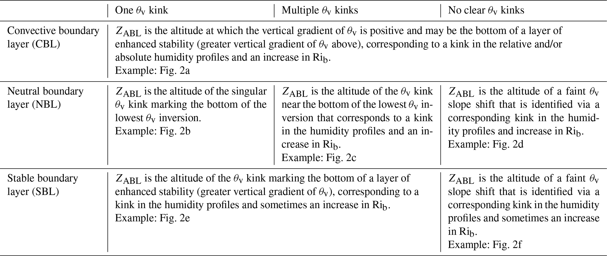
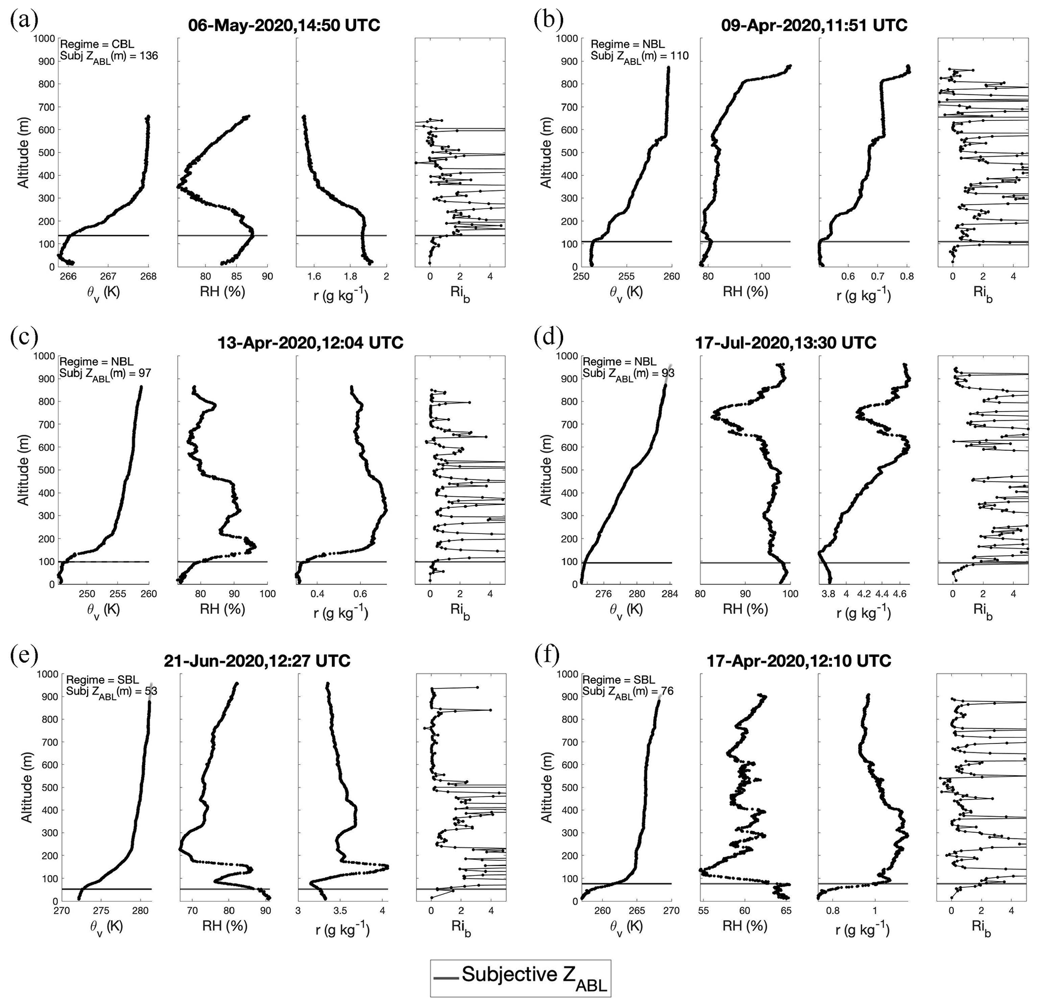
Figure 2For each flight shown here, the θv profile is plotted in the left panel, the RH and mixing ratio profiles are plotted in the middle two panels, and the Rib profile is plotted in the right panel. Subjective ZABL is marked with a horizontal black line in each panel and is written, along with stability regime, on the left panel. (a) Example of a CBL case. (b–d) Examples of NBL cases. (e, f) Examples of SBL cases.
Table 3 outlines the subjective criteria applied to determine ZABL depending on stability regime, which are separated depending on how many kinks there are in the θv profile that might indicate the entrainment zone. The term “kink” refers to a dramatic shift in slope (i.e., drastic change in vertical gradient). The primary methods applied to determine ZABL are those in which there are either one or two θv kinks, where we rely most heavily on the θv profile, and secondarily on the humidity and Rib profiles. For SBL cases, the humidity profiles often provide more insight than the Rib profile in identifying ZABL. In only a few especially difficult cases, we relied primarily on the Rib profiles. Figure 2 shows some examples of the subjective method applied.
When applying the above criteria, ZABL for the majority of cases (about 85 %) was clearly identifiable (i.e., relevant θv and humidity kinks were at the same altitude). For the other cases, ZABL was more ambiguous (e.g., Figs. S9, S12, S28, S34, S40, S42, S44, S48, S54, and S62 in the Supplement), meaning there were multiple features that one could argue marked the ABL top (i.e., the θv and humidity kinks that could both be interpreted as ZABL were at different altitudes). In these instances, depending on which feature is chosen, ZABL could differ by on average about 10–30 m, but preferential treatment is given to the kink that also corresponds to an increase in Rib. Additionally, if kinks in the RH and mixing ratio profiles occur at different altitudes, preferential treatment is given to the kink that occurs at the same altitude as that in the θv and/or Rib profiles. Following this, we determine the uncertainty in the subjective ZABL to be less than 30 m. Uncertainty in the height of a kink in an individual profile is only subject to the vertical averaging procedure and sensor response time, and thus it is on the order of only ∼ 1 m.
2.4 Objective identification of atmospheric boundary layer height
The strength of the subjective method described above is the knowledge of the expert, which cannot be automated (outside of possibly a machine learning algorithm, which would be costly and may still not be fully reliable). However, such expert knowledge and the time necessary to individually assess profiles is not always available. Thus, an automated method may often be preferred. Four such methods for objectively determining ZABL are applied and evaluated. Each of these methods relies on profiles of either or Rib, some in combination with the θv and/or wind speed profiles. Because the and Rib profiles are calculated over an altitude range of 30 m with 5 m resolution, objective ZABL detection methods which ultimately rely on these profiles can be determined with a resolution of 5 m. If they ultimately rely on the θv or wind speed profiles, ZABL can be determined with 1 m resolution. Figure 3 shows the application of all objective methods for an SBL and NBL case. A CBL case is not shown, as there were only two CBLs identified in the DH2 profiles, and they are rare in the central Arctic.
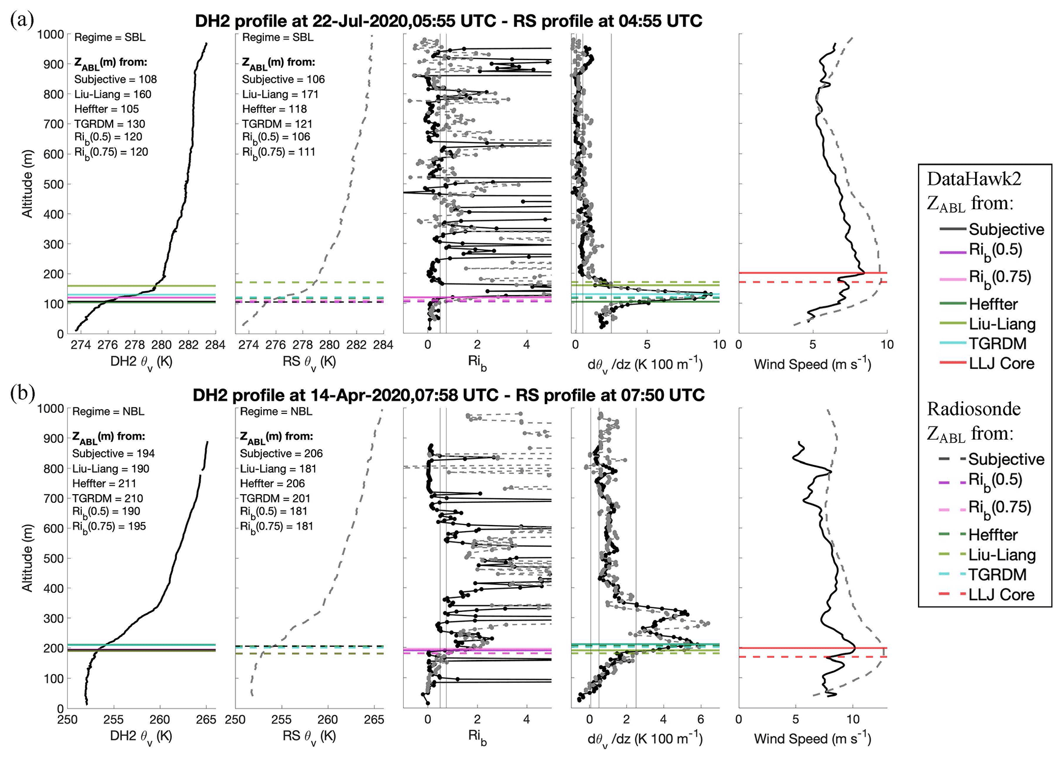
Figure 3Demonstration of ZABL identification using all objective methods on both the DH2 (represented by solid lines) and corresponding radiosonde (represented by dashed lines) for an (a) SBL and (b) NBL case. From left to right the following profiles are shown: θv profile from the DH2, θv profile from the radiosonde, Rib profiles from the DH2 (solid black) and the radiosonde (dashed grey), profiles from the DH2 (solid black) and the radiosonde (dashed grey), and wind speed profiles from the DH2 (solid black) and radiosonde (dashed grey). The legend on the right indicates the ZABL detection method associated with each horizontal line in the figure. The LLJ core is not in itself a ZABL detection method but plays into the Liu–Liang method, and thus it is included. Each ZABL is written on the corresponding platform's θv profile.
2.4.1 Liu–Liang method
The application of the Liu–Liang method depends on whether the profile includes a CBL, SBL, or NBL, which is determined using Eqs. (2)–(4). To implement the Liu–Liang method for a CBL profile, we first find the lowest altitude at which θv exceeds its the lowest DH2 value by 0.1 K. Then, ZABL is identified at the next lowest altitude in which exceeds 0.05 K (100 m)−1 (Liu and Liang, 2010). For an NBL, ZABL is identified as the altitude at which first exceeds 2.5 K (100 m)−1, which is adapted from a threshold of 0.05 K (100 m)−1 used in Liu and Liang (2010), as this threshold was found to be inappropriate for the current dataset (ZABL found with the original threshold was always far too low). The basis of this method is to identify the entrainment zone at the top of the ABL through an increased value of . The need for a greater threshold for NBL height identification in the current study is likely because the vertical resolution of sounding data used in the development of the Liu–Liang method was ∼ 40–50 m (Liu and Liang, 2010), which would result in a much smoother profile than what is possible with the DH2 data. However, it would not make sense to interpolate the DH2 profiles to a resolution of 40–50 m before applying the Liu–Liang method, as this would eliminate the ability the identify key features in the often shallow Arctic ABL.
For an SBL, the Liu–Liang method searches for a potential ZABL associated with either minimal turbulence due to the lack of buoyancy within the ABL or greater turbulence in the ABL due to the presence of wind shear (Liu and Liang, 2010), with both being scenarios that may dictate ZABL for an SBL (Stull, 1988). Thus, SBL height is defined as either the top of the bulk stable (θv inversion) layer starting from the ground or the height of the LLJ maximum if present, whichever is lower (Liu and Liang, 2010). The top of the bulk stable layer is identified where the surface-based θv inversion has consistently diminished, and LLJ presence is identified by searching for wind speeds reaching a maximum that is at least 2 m s−1 stronger than the local minima above and below (Stull, 1988; Liu and Liang, 2010). For greater detail on these methods and the guiding equations, see Liu and Liang (2010). Figure S1 shows an example of the Liu–Liang method applied to a case for each stability regime.
2.4.2 Heffter method
The Heffter method uses θv difference across a θv inversion (dθv) as an indication of ZABL (Sivaraman et al., 2013), by identifying the lowest θv inversion layer where is greater than 0.5 K (100 m)−1 throughout the θv inversion and dθv is at least 2 K (Heffter, 1980; Pesenson, 2003; Sivaraman et al., 2013). Within this θv inversion, the altitude at which θv first becomes more than 2 K greater than θv at the bottom of the θv inversion is labeled as ZABL (Marsik et al., 1995; Delle Monache et al., 2004; Snyder and Strawbridge, 2004; Sivaraman et al., 2013).
For a CBL or NBL, this method is meant to determine the altitude of the elevated θv inversion marking the entrainment zone between the well-mixed ABL and free atmosphere (Pesenson, 2003). For an SBL, this method determines where the change in strength of the surface θv inversion marks the transition from the ABL to residual layer (if one exists) or free atmosphere above (Stull, 1988). For greater detail on this method and the guiding equations, see Heffter (1980) or Sivaraman et al. (2013). Figure S2 in the Supplement shows an example of the Heffter method applied to a case for each stability regime.
2.4.3 Virtual potential temperature gradient maximum (TGRDM) method
The final -based method used to find ZABL is the virtual potential temperature gradient maximum (TGRDM) method (Dai et al., 2014). Since the ABL is typically capped by a well-defined θv inversion layer (Stull, 1988), even in a weakly stable case, we expect to see a local maximum in the profile at this point. By finding the maximum in the profile, the altitude at which the θv inversion is at its strongest and weakens above is identified. To apply this method, local maxima in the profile where is at least 1.75 K (100 m)−1 greater than the local minimum above are identified. ZABL is set to the altitude of this lowest peak. Figure S3 in the Supplement shows an example of the TGRDM method applied to a case for each stability regime.
2.4.4 Bulk Richardson number method
Finally, a bulk Richardson number method for finding the ABL top is applied by determining the altitude at which Rib exceeds a threshold value, which indicates where turbulence was likely no longer able to form in a laminar atmosphere. Previous literature suggests a wide range of critical values, with 0.25 (Stull, 1988) being the most widely accepted value, though a value of 0.5 is also often used (Sivaraman et al., 2013; Zhang et al., 2014). To determine a viable threshold value for the identifying ZABL in the DH2 data, a comparison between ZABL determined from a range of threshold values (we used 0.25, 0.5, 0.75, 1.0, 1.25, and 1.5) and the subjective ZABL was conducted. In identifying ZABL from these different threshold values, the level above which Rib was consistently greater than the threshold value was found. For this dataset, four consecutive data points (20 m) were required to be above the threshold value. We include this requirement due to the method of calculating Rib over a rolling 30 m range, rather than always with the ground as the reference layer, as it is possible for Rib to locally exceed the threshold but still be within the ABL. Thus, only when the Rib consistently exceeds the threshold, indicating that the bulk likelihood for turbulence has ceased, can we be confident that the top of the ABL has been reached.
Thus, the bottom of the lowest 20 m thick layer in which Rib exceeds the threshold value is identified as ZABL. The threshold values deemed to identify ZABL closest to that identified by the subjective method was 0.5 followed by 0.75. Therefore, further ZABL presented using the Rib method is calculated with threshold values of 0.5 (hereafter called Rib(0.5)) and 0.75 (hereafter called Rib(0.75)). Figure S4 in the Supplement shows an example of the Rib method applied to a case for each stability regime.
2.5 Applying the objective methods to radiosonde profiles
As discussed above, some of the objective methods used in this study were modified from their original descriptions to better work with the Arctic UAS data. Primarily, this includes changing the altitude range for determining stability regime, adjusting the threshold for calculating Liu–Liang NBL height, adding the 1.75 K (100 m)−1 criterion to the TGRDM method, and choosing the best threshold values and specifying the necessary vertical distance for the Rib method. These adaptations are necessary in part because previous implementations involved analysis of radiosonde profiles, which have a lower vertical resolution than the DH2 profiles, and in mid-latitude locations, where the ABL structure is often quite different than that observed in the Arctic. Thus, profiles of θv, humidity, and wind speed from the balloon-borne radiosondes that were launched at least four times per day from the deck of the Polarstern (Maturilli et al., 2021) during MOSAiC are leveraged to determine if the objective methods used to identify ZABL from the UAS data are robust across platforms, despite differences in sampling methods.
To do this, radiosonde profiles with launch times closest to the DH2 flight times (within at most ∼ 3 h) are used, repeating the same processes for subjective and objective ZABL identification and comparison. In eight instances, there were two DH2 flights in closest time proximity to the same radiosonde launch, and thus we use data from a total of 57 different radiosonde profiles. The specs for the Vaisala RS41-SGP sensor, which recorded the radiosonde variables, are the same as those listed in Table 2 for the DH2's RSS421 sensor, with the addition of pressure, temperature, and humidity uncertainty of 1.0 hPa, 0.3 ∘C, and 4 %, respectively, and a wind uncertainty and resolution of 0.15 and 0.1 m s−1, respectively, for velocity and of 2∘ and 0.1∘, respectively, for direction. The radiosonde samples had a frequency of 1 Hz and an approximate climb rate of 5 m s−1, which results in data with a vertical resolution of ∼ 5 m. Altitude measurements are calculated with the hydrostatic equation using the initial pressure at 10 m. Before proceeding with analysis, profiles of temperature, wind, and humidity from the radiosondes were visually compared to those from the corresponding DH2 flight to confirm that the measurements were similar to each other.
Prior to applying the objective methods, data below 23 m altitude were removed, as the lowest part of the radiosonde profiles were found to show inaccurately warm temperatures for several cases (Maturilli et al., 2021), due to the Polarstern acting as a “heat island.” Additionally, in some cases the radiosonde data showed anomalously warm measurements some distance above 23 m, which is assumed to be the result of the balloon passing through the Polarstern's exhaust plume. These measurements were adjusted by interpolating the temperature between the closest good measurements above and below where the radiosonde was presumably in the ship's plume. Applying these adjustments means that radiosonde data near the surface are not available for the determination of the stability regime. Therefore, we adapt the methods applied to the DH2 data in Eqs. (2)–(4) and instead calculate dθv between the lowest radiosonde measurement and 30 m above or the subjective ZABL if it is lower. We then compare this dθv to the appropriate threshold value, δs, that is equal to (0.2 K/40 m = 0.005 K m−1) times the Δz used. For example, if the Δz of 30 m is used, the value of δs is 0.15 K. These adaptations in themselves do not result in the identification of a different stability regime than is found in the DH2 profiles; instead, differences in stability regime between the two platforms may result from the lack of near-surface observations from the radiosonde or a change in atmospheric structure between the two corresponding launches.
Figure 3 shows two examples (one SBL and one NBL) of all of the objective methods applied to both a DH2 flight and its corresponding radiosonde. These examples show that the subjective ZABL identified using the DH2 and radiosonde data are similar (differing by only 2 m for the SBL and 12 m for the NBL) and that the objective methods reveal a similar outcome when applied to the radiosonde data as they do for the DH2 data for both cases. Similar figures for all DH2 and radiosonde profiles used in this study can be found in Figs. S5–S69 in the Supplement.
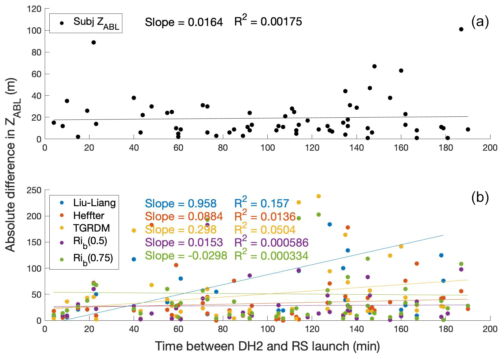
Figure 4Absolute difference between subjective ZABL from the DH2 and subjective ZABL from the radiosonde closest in time to the DH2 launch (black dots, a) and absolute difference between objective ZABL from the DH2 and objective ZABL from the radiosonde closest in time to the DH2 launch (colored dots, b) versus absolute time difference in minutes between the DH2 and radiosonde launches. A few outlier points are not shown, as they lie outside the range of the y axis. Lines of best fit are included for the subjective ZABL and for each objective method, and the slope and R2 value of each line is written next to the legend.
While the radiosonde and DH2 profiles generally exhibit a similar structure due to the close time and space proximity (the radiosondes were launched < 100 m from the DH2 flights), the subjective ZABL identified in those profiles differ by 1–101 m. In general, the deviation between ZABL from the DH2 and the radiosonde increases with increasing time proximity. Figure 4 shows the absolute difference between DH2 and radiosonde subjective ZABL (Fig. 4a), as well as the absolute difference between the DH2 and radiosonde objective ZABL for each method (Fig. 4b) as a function of time difference in minutes between the DH2 and radiosonde launch. The best fit linear regression for each method shows that as time between the DH2 and radiosonde launch increases, the differences in ZABL increase as well (though minimally). However, the increase in absolute difference between subjective ZABL from the DH2 and radiosonde as time between the launches increases is not significant at the 5 % significance level (probability value of 0.74). Therefore, we are confident that ZABL does not significantly change for DH2 and radiosonde launches up to 3.16 h apart, which justifies the use of the radiosonde closest in time to each DH2 to test if there is similar efficacy of the different objective methods.
3.1 Efficacy of objective ZABL identification methods
Whereas the objective methods all rely on information from one variable (or two, in the case of the Liu–Liang method for an SBL), the subjective method uses a combination of methods which can only be weighted properly by visual analysis. This is why the subjective method arguably results in a more accurate ZABL identification and provides a good basis for comparison with ZABL identified by the objective methods.
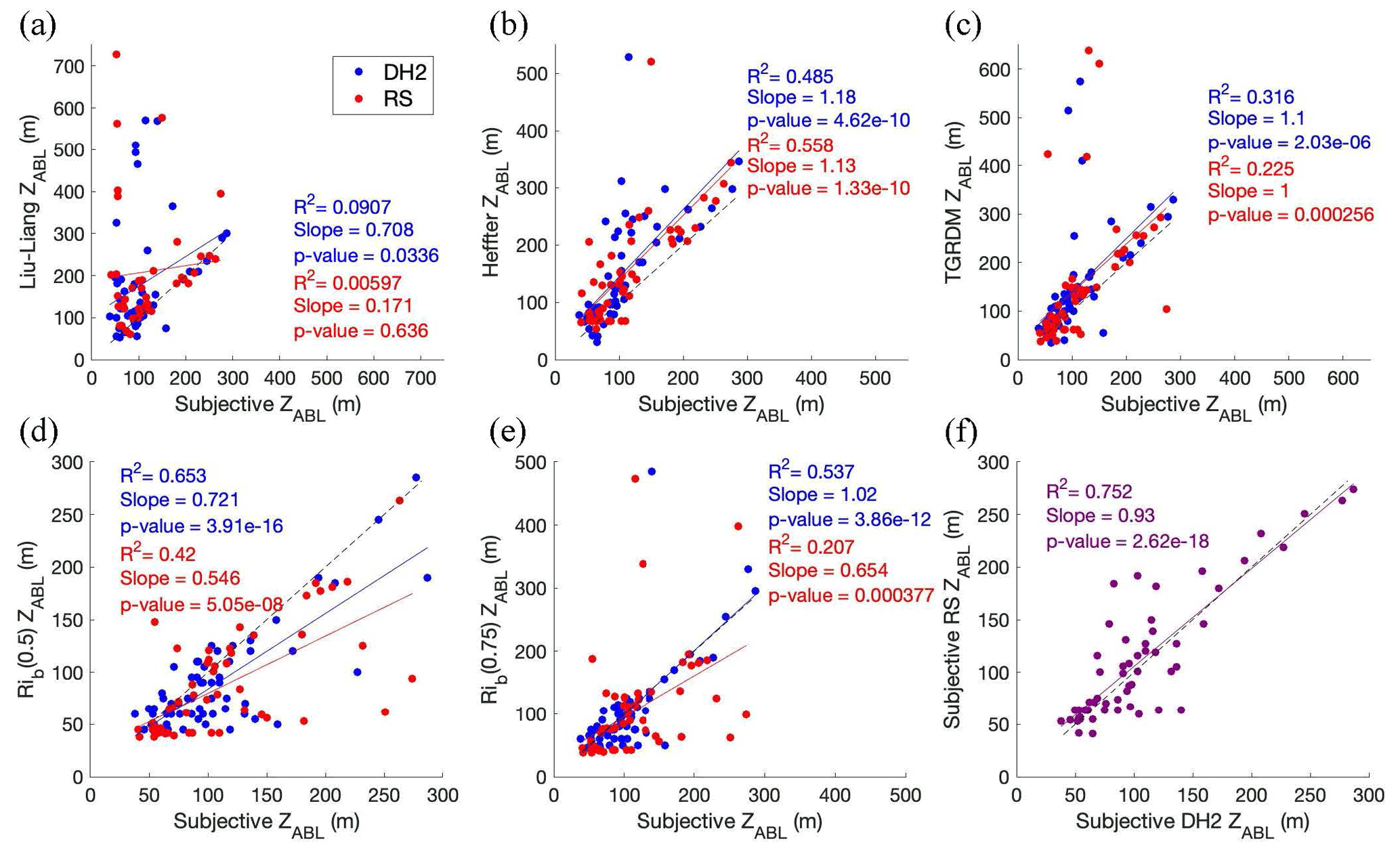
Figure 5Relationships between subjective ZABL and objective ZABL from the (a) Liu–Liang method (50 DH2 samples and 40 RS samples), (b) Heffter method (61 DH2 samples and 53 RS samples), (c) TGRDM method (62 DH2 samples and 55 RS samples), and (d, e) Rib method (65 DH2 samples and 57 RS samples). Blue dots represent DH2 data and red dots represent radiosonde data. The solid blue line (solid red line) in each panel is the line of best fit for the DH2 (radiosonde) data. (f) Relationship between subjective ZABL from the radiosonde and subjective ZABL from the DH2 with line of best fit in purple (57 samples). Each panel is overlaid by the corresponding R2, slope value, and p value. The dashed black line in each panel is a line with slope of 1.00 and y intercept of 0, for reference.
To determine how well the different objective methods worked, ZABL identified by each objective method is compared to the subjective ZABL. Figure 5 shows scatter plots comparing the objective to the subjective ZABL in each case, along with the associated best fit linear regression, coefficient of determination (R2), slope, and probability value (p value) resulting from a paired two sample t test. For instances in which there were two DH2 flights in closest time proximity to the same radiosonde launch, the results from that radiosonde profile are plotted only once.
The R2 value demonstrates how much of the variation in objective ZABL can be explained by the difference in subjective ZABL. Slope values (m) are also included to help evaluate the level of correspondence between the subjective and objective ZABL by comparison to an ideal value of m = 1.00. Additionally, looking at the intercept combined with the slope value tells us whether the objective method tends to overestimate or underestimate ZABL compared to the subjective method. Lastly, the p value tells us whether the relationship between subjective and objective ZABL can be considered statistically significant at the 5 % significance level (a p value less than 0.05 indicates that there is a 95 % chance the relationship is due to true correlation).
Based on the DH2 data in these scatter plots, the method that gives the greatest R2 is the Rib(0.5) method (R2 = 0.653, Fig. 5d), followed by the Rib(0.75) method (R2 = 0.537, Fig. 5e). These are followed closely by the Heffter method (R2 = 0.485, Fig. 5b). The TGRDM method has the fourth-highest R2 (R2 = 0.316, Fig. 5c). The only objective method with a very low R2 is the Liu–Liang method (R2 = 0.0907, Fig. 5a). The slope values for all methods fall within m = 1.00 ± 0.30, the closest to 1.00 being the Rib(0.75) method (m = 1.02), followed by the TGRDM method (m = 1.10) and Heffter method (m = 1.18). These slope values greater than 1.00 and positive intercept indicate that these methods generally overestimate ZABL when applied to the DH2 data, compared to the subjective ZABL. The results of the Rib(0.5) method and the Liu–Liang method, however, are more complex, as the slope values are both less than 1.00 (m = 0.721 and 0.708, respectively), but the intercepts are both positive. This indicates that these methods overestimate ZABL for a shallow ABL, but underestimate it for a deep ABL when applied to the DH2 data. Comparing the p values for all relationships to the 5 % significance level, the relationship between subjective and objective ZABL can be considered significant for every method (p value is less than 0.05). These p values follow the same order as the R2 values, with the lowest p value found for the Rib(0.5) (indicating the highest significance) and the highest p value for the Liu–Liang method (indicating the lowest significance).
The radiosonde data (referred to as “RS” in Fig. 5) give a slightly different conclusion. Here, the method that gives the greatest R2 is the Heffter method (R2 = 0.558, Fig. 5b), followed by the Rib(0.5) method (R2 = 0.420, Fig. 5d). The Rib(0.75) method and the TGRDM method have lower R2 (R2 = 0.207 and 0.225 in Fig. 5e and c, respectively). As was the case for the DH2 data, the only objective method with a very low R2 is the Liu–Liang method (R2 = 0.00597, Fig. 5a), which is also echoed by a slope value far from 1.00 (m = 0.171). The slope values for the rest of the methods are not as close to 1.00 as they are for the DH2 data, but they all fall within m = 1.00 ± 0.50. The TGRDM has a slope value of m = 1.00, and the method with the next closest value to 1.00 is the Heffter method at m = 1.13. Both of these methods have a positive intercept, which indicates that these methods tend to overestimate ZABL when applied to the radiosonde data used in the current study. The rest of the methods have a slope of less than 1.00 and positive intercept, indicating that they tend to overestimate ZABL for a shallow ABL but underestimate it for a deep ABL when applied to the radiosonde data used in the current study. However, as R2 for the Liu–Liang method is very low, this indicates that there is not much correlation between the objective and subjective ZABL for this method, and thus analysis of the slope does not provide reliable information. Lastly, the p values follow the same order as the R2 values, with the lowest p value found for the Heffter method (indicating the highest significance) and the highest p value for the Liu–Liang method (indicating the lowest significance). Unlike the DH2 results, for the radiosonde the p values for all relationships compared to the 5 % significance level show that the relationship between subjective and objective ZABL can be considered significant for every method except the Liu–Liang method, in which the p value is greater than 0.05.
Lastly, Fig. 5f compares subjective ZABL from the radiosondes to subjective ZABL from the DH2. The high R2 (0.752) indicates a rather strong correlation between subjective ZABL from both platforms, which demonstrates that ZABL usually did not change much between the DH2 and radiosonde launches in each case. Interestingly, there is enhanced deviation from the line of best fit for a shallower ABL and better agreement for a deeper ABL. However, this might simply be due to the greater number of samples with ZABL below ∼ 200 m. The very low p value of 2.62 × 10⁻¹⁸ demonstrates the high significance in the relationship between ZABL from the DH2 and radiosondes.

Figure 6Relationships between subjective ZABL and objective ZABL for only stable cases (top) and only neutral cases (bottom) from the (a, f) Liu–Liang method (20 DH2 and 23 RS samples for SBL cases; 28 DH2 and 17 RS samples for NBL cases), (b, g) Heffter method (30 DH2 and 35 RS samples for SBL cases; 30 DH2 and 18 RS samples for NBL cases), (c, h) TGRDM method (31 DH2 and 35 RS samples for SBL cases; 29 DH2 and 20 RS samples for NBL cases), and (d, e and i, j) Rib method (31 DH2 and 35 RS samples for SBL cases; 32 DH2 and 22 RS samples for NBL cases). Blue dots represent DH2 data, and red dots represent radiosonde data. The solid blue line (solid red line) in each panel is the line of best fit for the DH2 (radiosonde) data. Each panel is overlaid by the corresponding R2, slope value, and p value. The dashed black line in each panel is a line with slope of 1.00 and y intercept of 0, for reference.
Figure 6 shows the results presented in Fig. 5 but separated by stability regime, where the top half shows results for only SBLs, and the bottom half shows results for only NBLs. One primary takeaway from separating the results into stability regime is that for both platforms the TGRDM method performs better for SBLs than it does for NBLs. Similarly, the Heffter method performs better for SBLs than NBLs for the DH2 data and performs similarly for the radiosonde data. This discrepancy is likely because these two methods search for a θv inversion to identify ZABL, which is often more defined for an SBL than NBL. Next, for the DH2 data, the Rib methods show less dependency on stability, with rather high R2 for both regimes; however, the higher threshold performs better for NBL cases. Additionally, when splitting into stability regimes, the discrepancy between DH2 and radiosonde results increases for some methods. For example, the Rib method has more outliers for radiosonde NBL cases (Fig. 6i and j), causing R2 to be rather low. For this category, the Rib(0.5) method performs better, suggesting that the lower threshold value is more robust across platforms. Lastly, the Liu–Liang method, aside from a few outliers, performs rather well for NBL cases (Fig. 6f).
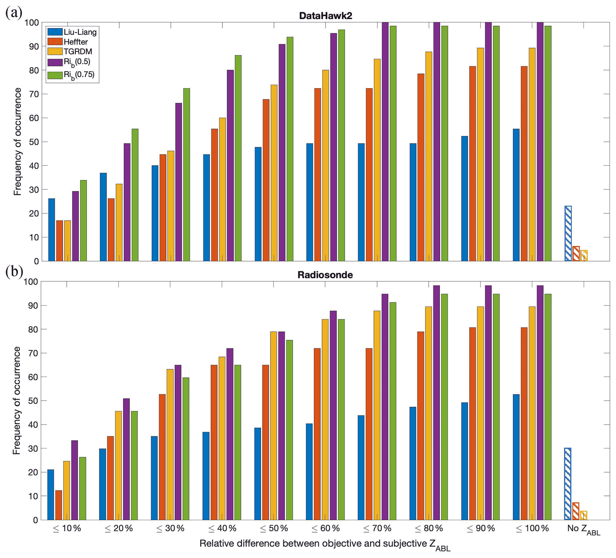
Figure 7Bar plot showing what percent of (a) DH2 cases and (b) radiosonde cases give an objective ZABL within different relative difference ranges from the subjective ZABL using the different objective methods. Plot also shows the percent of cases for each method where no ZABL is found (labeled as “No ZABL”).
Additional analysis was completed to assess the cumulative frequency distribution for the difference in objective ZABL relative to the subjective ZABL. To do this, relative difference between the objective and subjective ZABL in each case and for each method was determined. These results are included in Fig. 7a for the DH2 profiles and in Fig. 7b for the radiosonde profiles. For example, about 26 % of the time, the Liu–Liang ZABL was within 10 % of the subjective ZABL for the DH2 data.
Table 4Summary of the features that lead to failure by each objective method, along with examples of DH2 cases that exemplify each failure, which can be found in the figures in the Supplement. The last column indicates the figures in the Supplement associated with cases in which the objective ZABL had a greater than 50 % difference from the subjective ZABL or no objective ZABL was found.
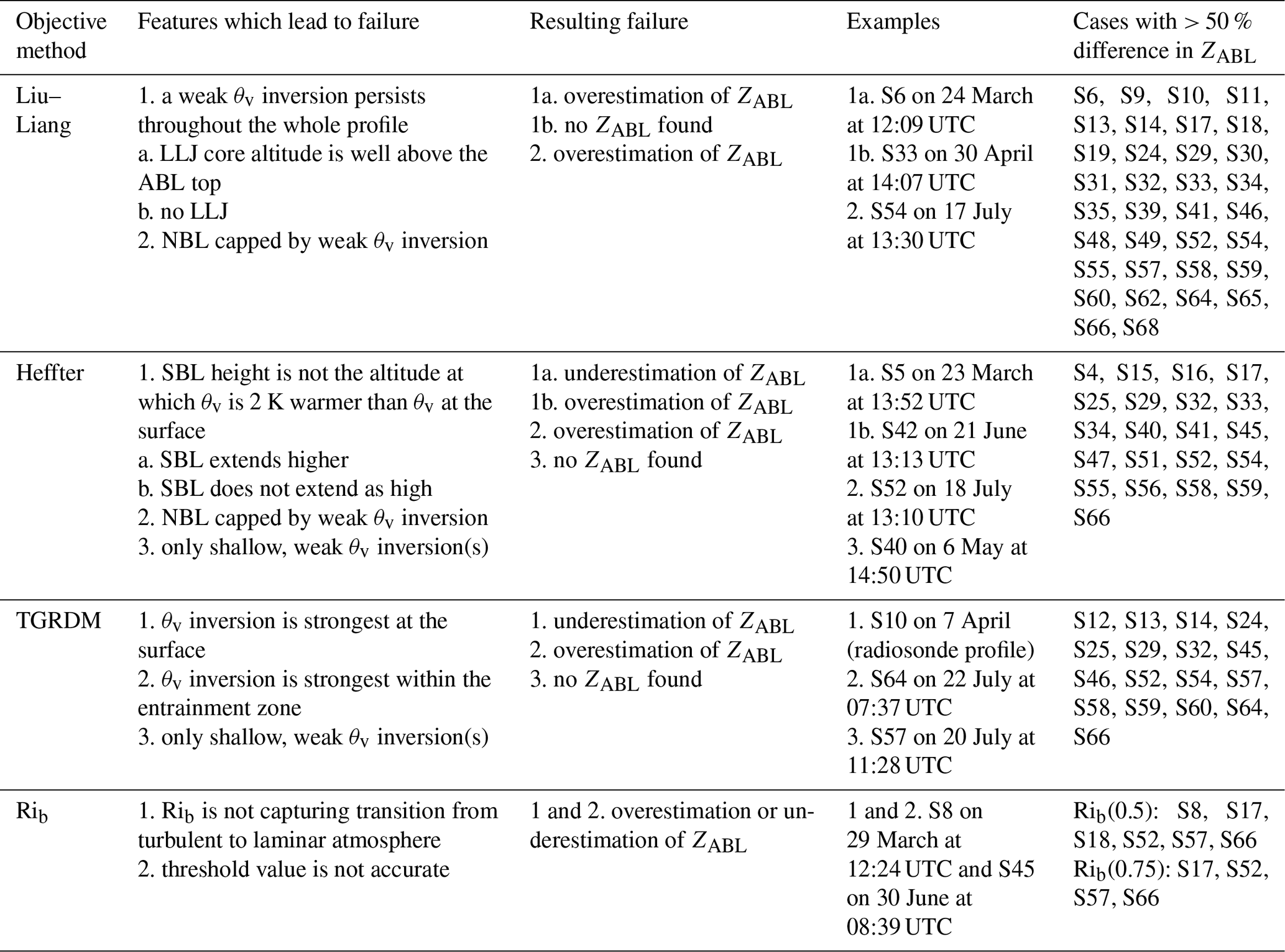
Figure 7a shows that for the DH2 profiles the Rib(0.75) method results in the highest percent of cases within 10 % of the subjective ZABL, followed by the Rib(0.5) method. Interestingly, the Liu–Liang method results in the third highest percent of cases within 10 % of the subjective ZABL. However, the Liu–Liang method falls behind other methods as the relative difference range is increased above 20 %. Additionally, the Liu–Liang method has the highest percent of cases in which no ZABL is found at all for the DH2 profiles, as well as about 20 % of cases that have greater than 100 % difference from the subjective ZABL. This trend indicates that while the Liu–Liang method sometimes works to find a ZABL close to the subjective ZABL, it also fails to find a ZABL close to the subjective ZABL or to find any ZABL in many cases. The primary reason for the failure of the Liu–Liang method, which is listed in Table 4 and discussed further in Sect. 3.2 below, is the high prevalence of a weak θv inversion that persists throughout the entire lower atmosphere in the Arctic. Another important finding is that the Rib method using either threshold value never fails to find a ZABL, and the number of cases within each relative difference range is greater for the Rib method than that for all other methods.
The information presented in the bar graph for the radiosonde profiles (Fig. 7b) leads to a similar conclusion. As for the DH2 profiles, the Rib method results in the highest percent of cases within 10 % of the subjective ZABL (but for this platform, the Rib(0.5) method does best). Here, the Liu–Liang method results in the fourth highest percent of cases within 10 % of the subjective ZABL and performs more poorly as the relative difference range is increased. The Liu–Liang method also has the highest percent of cases in which no ZABL is found at all, followed by the Heffter and TGRDM methods, which was also true for the DH2 data. As for the DH2, there are no radiosonde cases in which the Rib method with either threshold value finds no ZABL. The main difference between Fig. 7b of the radiosonde data and Fig. 7a of the DH2 data is that while the Rib(0.75) method applied to the DH2 data was always more successful than the Rib(0.5) method for relative difference ranges below 70 %, for the radiosonde data the Rib(0.5) method proves to always be more successful than the Rib(0.75) method. We suspect that this results from the radiosonde data being more smoothed, which produces less sporadic Rib values as the atmosphere transitions from the ABL to the free atmosphere compared to the less smoothed DH2 data. This smoothing of the radiosonde data is applied by the Vaisala software to remove any effect of the chaotic pendulum swing directly after launch while the wire unwinds. Thus, a lower threshold Rib value may be better applicable when more smoothing or filtering procedures are applied to a dataset.
Figures S70 and S71 in the Supplement show the results presented in Fig. 7 but separated by stability regime, where Fig. S70 shows results for only SBLs and Fig. S71 shows results for only NBLs. The primary takeaways from separating the results into stability regime is that for both the DH2 and radiosonde, the Rib method has the most cases and the Liu–Liang method has the least cases with objective ZABL within 10 % of the subjective ZABL for SBLs, though the Heffter and TGRDM methods also do well. For NBLs, the Liu–Liang method actually has the most cases with objective ZABL within 10 % of the subjective ZABL, followed by the Rib method for both platforms.
After comparing ZABL from the different objective methods to the subjective ZABL for both the DH2 and the radiosondes (Figs. 5 and 7), it is found that, with the exception of the Liu–Liang method, all other methods generally provide a reasonable estimate of ZABL for both datasets, with the Rib method being most favorable. This is in agreement with Seibert et al. (2000), Dai et al. (2014), and Zhang et al. (2014), who found an Rib-based method to be preferred when mechanically produced turbulence dominates, as is true in the central Arctic (Brooks et al., 2017). Additionally, the efficacy of each method is similar for the DH2 and the radiosonde data, as is indicated by similar patterns in the scatter plots (Fig. 5) and bar plots (Fig. 7), despite occasional differences in radiosonde versus DH2-based ZABL estimates, which likely result from the differences in sampling methods between the two platforms. Most specifically, the DH2 samples very close to the surface (∼ 5 m) in most cases, and thus it observes important ABL features that support accurate stability and ZABL identification, whereas the radiosonde, which only samples down to 23 m at the lowest, may miss these features. Additionally, the DH2 samples with higher vertical resolution (due to higher time resolution of instrumentation and slower climb rate), again contributing to its ability to record complex fine-scale features that the radiosonde might miss. However, the similarity in efficacy of the objective methods between both platforms supports the fact that the objective ZABL identification methods that were adjusted using the high-resolution DH2 data are indeed robust across platforms with different sampling methods.
This is further explored by re-running the analysis with DH2 profiles averaged over 5, 10, and 20 m bins instead of 1 m bins to determine how sensitive the efficacy of the methods is to the vertical resolution of the data. When comparing objective ZABL found using the coarser data to the original subjective ZABL for each method, the F test reveals that the R2 values generally do not differ significantly from those found using 1 m binned data at the 5 % significance level. The only exceptions are the Liu–Liang method at all larger bin sizes and the Heffter method when using a 10 or 20 m bin size, which all manifest in lower R2 value than those found using 1 m binned data. This reveals that the Liu–Liang method performs even more poorly at lower vertical resolution and that the Heffter method starts to perform more poorly at a vertical resolution of 10 m. On the other hand, the Rib and TGRDM methods remain just as successful when vertical resolution is reduced, and the preferred Rib threshold value does not appear to depend on vertical resolution. For vertical resolution of 30 m or coarser, the altitude range over which Rib is calculated would have to be increased, and at this point a lower threshold Rib value may be more applicable.
While we state an uncertainty in the subjective ZABL to be less than 30 m, this is only applicable to a handful of DH2 flights (∼ 15 %), whereas the majority have an uncertainty on the order of only ∼ 1 m due to the vertical averaging procedure and sensor response time. Therefore, we do not expect this uncertainty to make any significant effect on the results.
3.2 When the objective methods fail
Table 4 lists the most common features that cause each objective method to fail (meaning the objective ZABL is much different than the subjective ZABL), along with the corresponding failure (either overestimation or underestimation or no ZABL found) and an example of such a situation shown in the figures in the Supplement. As shown in Sect. 3.1, while the Liu–Liang method sometimes works well, it is not reliable across a wide range of different profile structures. Option 1a causes failure because the criteria are not met anywhere in the profile, meaning that the method reverts to using the LLJ core height as ZABL. However, the LLJ core was observed to usually be above the subjective ZABL (supported by Stull, 1988; Jakobson et al., 2013; and Mahrt et al., 2014). This cause for failure agrees with Dai et al. (2014), which found that using LLJ core height to define SBL top produces results inconsistent with those from other methods. The Liu–Liang method likely performs better for NBL cases (as is evident in Figs. 6 and S71) than SBL cases because the Liu–Liang method for an NBL is not dependent on the sufficient diminishment of the θv inversion or the presence or altitude of a LLJ.
Any of the other objective methods would be a good choice for objectively determining ZABL for a dataset similar to the DH2 and radiosonde datasets (high-resolution profiles in the central Arctic environment). However, each method still struggles in some situations. The primary downfall of the Heffter method is that it identifies ZABL as the point where θv is 2 K warmer than θv at the bottom of the θv inversion. Failures noted in options 1–3 in Table 4 all occur when this criterion does not accurately identify the ABL top. The primary downfall of the TGRDM method, as noted in options 1–2 in Table 4, is that the strongest point of the θv inversion is not always at the ABL top. The TGRDM method also fails to find any ZABL if there is no θv inversion strong enough to exceed the threshold necessary for ZABL identification as laid out in Sect. 2.4.3. Lastly, the failure of the Rib method occurs due to the difficulty of defining an accurate threshold value that correctly captures the likelihood of turbulence for all cases.
The last column in Table 4 lists the cases in which the objective ZABL differs by more than 50 % from the subjective ZABL for the DH2 data or no ZABL was found, which can be referenced in the figures in the Supplement for all examples of the profile structures that are not as conducive to the success of the different objective methods.
Aside from what is listed in Table 4, the objective methods may produce results different than those found by the subjective method due to the consideration of different variables. Primarily, none of the objective methods directly consider the profiles of RH or mixing ratio (of course, humidity is indirectly considered through the virtual potential temperature profiles). Additionally, the Liu–Liang method for a CBL or NBL, as well as the Heffter and TGRDM methods, do not consider wind shear in the identification of ZABL.
When applying these objective methods to a large dataset to automatically identify ZABL, it is recommended that some level of pre-screening is applied to flag cases that contain the features or structural patterns summarized in Table 4 that can objectively be identified and would make certain objective methods have difficulty identifying ZABL (for example, one can screen for whether the θv persists throughout the entire profile or where the θv maximum occurs) and choosing which objective method to use based on that. While not all features in Table 4 may be possible to pre-screen for, this list should at least help to identify some cases in which certain objective methods are likely to fail.
On the simplest level, one could choose which objective ZABL detection method to use based on stability regime. Given the results in Figs. 6, S70, and S71, the best choice to use for SBLs might be the Heffter method (highest R2 and higher frequency of cases within 10 % of the subjective ZABL when compared to NBL cases from both the DH2 and radiosonde data), and the best choice to use for NBLs might be the Rib method with either threshold value (highest R2 values from the DH2 data and higher frequency of cases within 10 % of the subjective ZABL when compared to SBL cases from both the DH2 and radiosonde data). However, when separating out the efficacy of the objective methods depending on stability regime, the Rib method has a combination of a high R2 values and a high percentage of cases with objective ZABL within 10 % of the subjective ZABL for both stability regimes, and thus this would be the best choice to apply to all profiles if one wanted to choose a single method, preferably with the threshold value of 0.5.
Overall, the objective methods are more likely to agree with each other as well as with the subjective ZABL for cases with more simplistic structures, such as those with strong θv inversions with a base at or just below the top of the ABL, those with LLJ core altitude at or just above the top of the ABL, and those with consistently and somewhat gradually increasing θv with altitude above the entrainment zone.
By comparing subjective ZABL identified visually in θv, humidity (both RH and mixing ratio), and Rib profiles to objectively determined ZABL, the performance of several published methods (i.e., Liu–Liang, Heffter, TGRDM, and Rib) are evaluated across 65 DH2 UAS profiles. When comparing objective to subjective ZABL for each DH2 case, the method that is most successful (combination of high R2 value, low p value, and slope close to 1.00) is the Rib method with either threshold value of 0.5 or 0.75 (Fig. 5). When calculating the percent of DH2 cases in which the objective ZABL is within certain relative difference ranges from the subjective ZABL, the Rib method is also most successful (Fig. 7). The Heffter and TGRDM methods also produce reasonable results according to Figs. 5 and 7. The only objective method that largely fails at accurately identifying ZABL is the Liu–Liang method.
In the process of applying these different objective methods to the DH2 data, some threshold values were modified to be better applicable to the UAS dataset. While these adjustments were made to best suit the 65 DH2 profiles analyzed in this study, which occurred between March and July of 2020, these adjustments should yield better results for identifying ZABL over sea ice during any season and location in the central Arctic. We hypothesize this because the ABL structures sampled by the DH2 in the current study were diverse and encompass the variety of ABL structures commonly observed in the central Arctic (which are typically shallow and either stable or neutral) throughout the entire year. Additionally, since the locations of the DH2 flights in this study range from deep in the Arctic pack ice to near the marginal ice zone, we are confident that the adjustments made will be applicable for identifying ZABL in either environment.
Testing these adjustments outside of the 65 DH2 flights, the modified techniques were also applied to the radiosonde profiles closest in time to each DH2 flight, to determine if the methods work similarly on data from another sensing platform with different sampling methods. Radiosonde profiles closest in time proximity to the DH2 flights were used under the assumption that the ABL structure would change minimally between the launch of the two platforms (supported by Fig. 4), and thus applying the methods of subjective and objective ZABL detection would lead to a similar conclusion. For the radiosonde data, the Heffter and Rib methods prove most successful in terms of having a high R2 value, low p value, and slope closest to 1.00 when compared to the other objective methods (Fig. 5). Additionally, the Rib method also proves most successful when looking at the percent of cases in which the objective ZABL was within different relative difference ranges for the radiosondes, as it did for the DH2 (Fig. 7). Once again, the only method that consistently provided unfavorable results is the Liu–Liang method. These similar conclusions demonstrate that the adapted objective methods are indeed robust across platforms despite differences in sampling method, which suggest that one can take the methods and apply them to UAS, radiosonde, or other profile data alike without having to tweak them.
These findings show that no single method works well 100 % of the time. Given this, the best way to accurately identify ZABL across a variety of conditions in the Arctic atmosphere is to visually analyze the θv, humidity, and Rib profiles for each case individually. However, as subjective identification is time consuming and requires expert knowledge of the physical processes that dictate ABL structure, in the case of large datasets that require automated processing techniques, the current study reveals that the Rib, Heffter, or TGRDM methods are most suitable for such a task, with the preferred method being the Rib method with threshold value of 0.5. For data with vertical resolution of 10 m or coarser, the Heffter method is no longer recommended. The Liu–Liang method does not provide consistent results in accurately identifying Arctic ZABL in many cases, especially for SBLs (Fig. S70). The most common occurrence of failure of the objective methods exists for NBLs capped by a weak θv inversion, and thus a clear θv slope change between the ABL and entrainment zone is difficult for automated methods to find. In such cases, the Rib method was found to be most reliable for identifying ZABL. A full list of features that cause each objective method to fail is provided in Table 4. The objective methods may also fail if the near-surface atmosphere is not well sampled, for example in the case of the radiosonde data; if ABL stability is defined by what is happening near the surface (e.g., a shallow convective layer), then this is missed by radiosonde profiles which only begin 23 m or higher, and stability regime could be incorrectly diagnosed. This highlights the value of platforms that can sample the near-surface atmosphere, such as the DH2. To accommodate the above problems, a semi-automatic approach may be beneficial in which one would apply all the recommended objective methods and visually inspect only the profiles for which the resulting ZABL diverges greatly.
The methods and results of this study for stability regime and ZABL identification are currently being applied to the entire year of radiosonde data collected during the MOSAiC expedition (October 2019 – September 2020) to create a data product containing year-long statistics on ABL characteristics in the central Arctic. Additional metrics, such as LLJ height and speed, and temperature inversion layer depth and strength will be included in this product for eventual publication. The value of the DH2 data and methods used in the current study comes from the uniqueness of the location and timing of the profiles collected. Therefore, these data provide a unique opportunity to evaluate any additional ZABL detection schemes that were not addressed in this study or that have yet to be developed and can be used to learn about the intricacies of additional structural components of the Arctic atmosphere such as the entrainment zone. Lastly, we are working to derive turbulence parameters from the DH2 fine-wire measurements, which will enhance the value of the DH2 data in ABL studies.
All DataHawk2 data used in this study are openly available from the National Science Foundation Arctic Data Center at https://doi.org/10.18739/A2KH0F08V (Jozef et al., 2021) as described in de Boer et al. (2022). The radiosonde data are available at the PANGAEA Data Publisher at https://doi.org/10.1594/PANGAEA.928656 (Maturilli et al., 2021). These data are subject to the MOSAiC Data Policy (Immerz et al., 2019) and will be openly available after 1 January 2023.
The supplement related to this article is available online at: https://doi.org/10.5194/amt-15-4001-2022-supplement.
GdB and JC planned the DH2 data collection and acquired funding. GJ and JC conducted DH2 flights. SD provided the radiosonde data. GJ, JC, and GdB conceptualized the analysis presented in this paper. GJ analyzed the data. GJ wrote the manuscript. JC, GdB, and SD reviewed and edited the manuscript.
The contact author has declared that none of the authors has any competing interests.
Publisher's note: Copernicus Publications remains neutral with regard to jurisdictional claims in published maps and institutional affiliations.
Data used in this paper were produced as part of RV Polarstern cruise AWI_PS122 and the international Multidisciplinary drifting Observatory for the Study of the Arctic Climate (MOSAiC) with the tag MOSAiC20192020. We thank all those who contributed to MOSAiC and made this endeavor possible (Nixdorf et al., 2021). Radiosonde data were obtained through a partnership between the leading Alfred Wegener Institute (AWI), the Atmospheric Radiation Measurement (ARM) User Facility, a U.S. Department of Energy facility managed by the Biological and Environmental Research Program, and the German Weather Service (DWD). Non-author contributors to DH2 design, data collection, and data processing include Dale Lawrence (Dept. of Aerospace Engineering Sciences, University of Colorado Boulder), Jonathan Hamilton (Dept. of Aerospace Engineering Sciences, University of Colorado Boulder; Cooperative Institute for Research in Environmental Sciences, University of Colorado Boulder; NOAA Physical Sciences Laboratory), Radiance Calmer (Cooperative Institute for Research in Environmental Sciences, University of Colorado Boulder; National Snow and Ice Data Center, University of Colorado Boulder), Brian Argrow (Dept. of Aerospace Engineering Sciences, University of Colorado Boulder; Integrated Remote and In-Situ Sensing, University of Colorado Boulder), Steven Borenstein (Dept. of Aerospace Engineering Sciences, University of Colorado Boulder; Integrated Remote and In-Situ Sensing, University of Colorado Boulder), Abhiram Doddi (Dept. of Aerospace Engineering Sciences, University of Colorado Boulder), Julia Schmale (Swiss Federal Institute of Technology Lausanne), and Andreas Preußer (University of Trier).
This research has been supported by the National Science Foundation (grant no. 1805569), the Cooperative Institute for Research in Environmental Sciences, the National Oceanic and Atmospheric Administration Physical Sciences Laboratory, and the Alfred Wegener Institute.
This paper was edited by Dominik Brunner and reviewed by three anonymous referees.
Alfred-Wegener-Institut Helmholtz-Zentrum für Polar- und Meeresforschung: Polar Research and Supply Vessel POLARSTERN operated by the Alfred-Wegener-Institute, Journal of Large-Scale Research Facilities, 3, A119, https://doi.org/10.17815/jlsrf-3-163, 2017.
American Meteorological Society: Bulk Richardson number. Glossary of Meteorology, https://glossary.ametsoc.org/wiki/Bulk_richardson_number (last access: 4 March 2022), 2012.
Andreas, E. L., Horst, T. W., Grachev, A. A., Persson, P. O. G., Fairall, C. W., Guest, P. S., and Jordan, R. E.: Parametrizing turbulent exchange over summer sea ice and the marginal ice zone, Q. J. Roy. Meteor. Soc., 136, 927–943, https://doi.org/10.1002/qj.618, 2010.
Banta, R. M., Pechugina, Y. L., and Newsom, R. K.: Relationship between Low-Level Jet Properties and Turbulence Kinetic Energy in the Nocturnal Stable Boundary Layer, J. Atmos. Sci., 60, 2549–2555, https://doi.org/10.1175/1520-0469(2003)060<2549:RBLJPA>2.0.CO;2, 2003.
Brooks, I. M., Tjernström, M., Persson, P. O. G., Shupe, M. D., Atkinson, R. A., Canut, G., Birch, C. E., Mauritsen, T., Sedlar, J., and Brooks, B. J.: The Turbulent Structure of the Arctic Summer Boundary Layer During The Arctic Summer Cloud-Ocean Study, J. Geophys. Res.-Atmos., 122, 9685–9704, https://doi.org/10.1002/2017JD027234, 2017.
Collaud Coen, M., Praz, C., Haefele, A., Ruffieux, D., Kaufmann, P., and Calpini, B.: Determination and climatology of the planetary boundary layer height above the Swiss plateau by in situ and remote sensing measurements as well as by the COSMO-2 model, Atmos. Chem. Phys., 14, 13205–13221, https://doi.org/10.5194/acp-14-13205-2014, 2014.
Dai, C., Gao, Z., Wang, Q., and Cheng, G.: Analysis of Atmospheric Boundary Layer Height Characteristics over the Arctic Ocean Using the Aircraft and GPS Soundings, Atmos. Ocean. Sci. Lett., 4, 124–130, https://doi.org/10.1080/16742834.2011.11446916, 2011.
Dai, C., Wang, Q., Kalogiros, J. A., Lenschow, D. H., Gao, Z., and Zhou, M.: Determining Boundary-Layer Height from Aircraft Measurements, Bound.-Lay. Meteorol., 152, 277–302, https://doi.org/10.1007/s10546-014-9929-z, 2014.
de Boer, G., Chapman, W., Kay, J. E., Medeiros, B., Shupe, M. D., Vavrus, S., and Walsh, J.: A Characterization of the Present-day Arctic Atmosphere in CCSM4, J. Climate, 25, 2676–2695, https://doi.org/10.1175/JCLI-D-11-00228.1, 2012.
de Boer, G., Calmer, R., Jozef, G., Cassano, J., Hamilton, J., Lawrence, D., Borenstein, S., Doddi, A., Cox, C., Schmale, J., Preußer, A., and Argrow, B.: Observing the Central Arctic Atmosphere and Surface with University of Colorado Uncrewed Aircraft Systems, Nat. Sci. Data, accepted, 2022.
Delle Monache, L., Perry, K. D., Cederwall, R. T., and Ogren, J. A.: In situ aerosol profiles over the Southern Great Plains cloud and radiation test bed site: 2. Effects of mixing height on aerosol properties, J. Geophys. Res.-Atmos., 109, D6, https://doi.org/10.1029/2003jd004024, 2004.
Esau, I. and Sorokina, S.: Climatology of the Arctic Planetary Boundary Layer, in: Atmospheirc Turbulence, Meteorological Modeling and Aerodynamics, edited by: Lang, P. R. and Lombargo, F. S., Nova Science Publishers, Inc., New York, 3–58, ISBN 978-1-60741-091-1, 2010.
Garratt, J. R.: Review: the atmospheric boundary layer, Earth-Sci. Rev., 37, 89–134, https://doi.org/10.1016/0012-8252(94)90026-4, 1994.
Georgoulias, A. K., Papanastasiou, D. K., Melas, D., Amiridis, V., and Alexandri, G.: Statistical analysis of boundary layer heights in a suburban environment, Meteorol. Atmos. Phys., 104, 103–111, https://doi.org/10.1007/s00703-009-0021-z, 2009.
Grachev, A. A., Fairall, C. W., Persson, P. O. G., Andreas, E. L., and Guest, P. S.: Stable Boundary-layer Scaling Segimes: The SHEBA Data, Bound.-Lay. Meteorol., 116, 201–235, https://doi.org/10.1007/s10546-004-2729-0, 2005.
Hamilton, J., de Boer, G., Doddi, A., and Lawrence, D.: The DataHawk2 Uncrewed Aircraft System for Atmospheric Research, Atmos. Meas. Tech. Discuss. [preprint], https://doi.org/10.5194/amt-2022-96, in review, 2022.
Heffter, J. L.: Transport layer depth calculations, in: Proceedings of the 2nd Joint Conference on Applications of Air Pollution Modelling, American Meteorological Society, 24–27 March 1980, New Orleans, LA, USA, American Meteorological Society, 787–791, 1980.
Immerz, A., Frickenhaus, S., von der Gathen, P., Shupe, M., Morris, S., Nicolaus, M., Schneebeli, M., Regnery, J., Fong, A., Snoeijs-Leijonmalm, P., Geibert, W., Rabe, B., Herber, A., Krumpen, T., Singha, S., Jaiser, R., Ransby, D., Schumacher, S., Driemel, A., Gerchow, P., Schäfer, A., Schewe, I., Ajjan, M., Glöckner, F. O., Schäfer-Neth, C., Jones, C., Goldstein, J., Jones, M., Prakash, G., and Rex, M.: MOSAiC Data Policy, Zenodo, https://doi.org/10.5281/zenodo.4537178, 2019.
Jakobson, L., Vihma, T., Jakobson, E., Palo, T., Männik, A., and Jaagus, J.: Low-level jet characteristics over the Arctic Ocean in spring and summer, Atmos. Chem. Phys., 13, 11089–11099, https://doi.org/10.5194/acp-13-11089-2013, 2013.
Jenkins, A. D., Paskyabi, M. B., Fer, I., Gupta, A., and Adakudlu, M.: Modelling the Effect of Ocean Waves on the Atmospheric and Ocean Boundary Layers, Enrgy Proced., 24, 166–175, https://doi.org/10.1016/j.egypro.2012.06.098, 2012.
Jozef, G., de Boer, G., Cassano, J., Calmer, R., Hamilton, J., Lawrence, D., Borenstein, S., Doddi, A., Schmale, J., Preußer, A., and Argrow, B.: DataHawk2 Uncrewed Aircraft System data from the Multidisciplinary drifting Observatory for the Study of Arctic Climate (MOSAiC) campaign, B1 level, Arctic Data Center [data set], https://doi.org/10.18739/A2KH0F08V, 2021.
Karlsson, J. and Svensson, G.: Consequences of poor representation of Arctic sea-ice albedo and cloud-radiation interactions in the CMIP5 model ensemble, Geophys. Res. Lett., 40, 4374–4379, https://doi.org/10.1002/grl.50768, 2013.
Krumpen, T., von Albedyll, L., Goessling, H. F., Hendricks, S., Juhls, B., Spreen, G., Willmes, S., Belter, H. J., Dethloff, K., Haas, C., Kaleschke, L., Katlein, C., Tian-Kunze, X., Ricker, R., Rostosky, P., Rückert, J., Singha, S., and Sokolova, J.: MOSAiC drift expedition from October 2019 to July 2020: sea ice conditions from space and comparison with previous years, The Cryosphere, 15, 3897–3920, https://doi.org/10.5194/tc-15-3897-2021, 2021.
Lawrence, D. A. and Balsley, B. B.: High-Resolution Atmospheric Sensing of Multiple Atmospheric Variables Using the DataHawk Small Airborne Measurement System, J. Atmos. Ocean. Tech., 30, 2352–2366, https://doi.org/10.1175/jtech-d-12-00089.1, 2013.
Lesins, G., Duck, T. J., and Drummond, J. R.: Surface Energy Balance Framework for Arctic Amplification of Climate Chang, J. Climate, 25, 8277–8288, https://doi.org/10.1175/JCLI-D-11-00711.1, 2012.
Liu, S. and Liang, X. Z.: Observed Diurnal Cycle Climatology of Planetary Boundary Layer Height, J. Climate, 23, 5790–5809, https://doi.org/10.1175/2010JCLI3552.1, 2010.
Lüpkes, C., Vihma, T., Birnbaum, G., and Wacker, U.: Influence of leads in sea ice on the temperature of the atmospheric boundary layer during polar night, Geophys. Res. Lett., 35, L03805, https://doi.org/10.1029/2007GL032461, 2008.
Mahrt, L., Vickers, D., and Andreas, E. L.: Low-Level Wind Maxima and Structure of the Stable Stratified Boundary Layer in the Coastal Zone, J. Appl. Meteorol. Clim., 53, 363–376, https://doi.org/10.1175/JAMC-D-13-0170.1, 2014.
Marsik, F. J., Fischer, K. W., McDonald, T. D., and Samson, P. J.: Comparison of Methods for Estimating Mixing Height Used during the 1992 Atlanta Filed Intensive, J. Appl. Meteorol. Clim., 34, 1802–1814, https://doi.org/10.1175/1520-0450(1995)034<1802:COMFEM>2.0.CO;2, 1995.
Maturilli, M., Holdridge, D. J., Dahlke, S., Graeser, J., Sommerfeld, A., Jaiser, R., Deckelmann, H., and Schulz, A.: Initial radiosonde data from 2019-10 to 2020-09 during project MOSAiC, Alfred Wegener Institute, Helmholtz Centre for Polar and Marine Research, Bremerhaven, PANGAEA [data set], https://doi.org/10.1594/PANGAEA.928656, 2021.
Mayer, S., Jonassen, M. O., Sandvik, A., and Reuder, J.: Profiling the Arctic Stable Boundary Layer in Advent Valley, Svalbard: Measurements and Simulations, Bound.-Lay. Meteorol., 143, 507–526, https://doi.org/10.1007/s10546-012-9709-6, 2012.
Nicolaus, M., Perovich, D., Spreen, G., Granskog, M., Albedyll, L., Angelopoulos, M., Anhaus, P., Arndt, S., Belter, H., Bessonov, V., Birnbaum, G., Brauchle, J., Calmer, R., Cardellach, E., Cheng, B., Clemens-Sewall, D., Dadic, R., Damm, E., Boer, G., Demir, O., Dethloff, K., Divine, D., Fong, A., Fons, S., Frey, M., Fuchs, N., Gabarró C., Gerland, S., Goessling, H., Gradinger, R., Haapala, J., Haas, C., Hamilton, J., Hannula, H.-R., Hendricks, S., Herber, A., Heuzé C., Hoppmann, M., Høyland K., Huntemann, M., Hutchings, J., Hwang, B., Itkin, P., Jacobi, H.-W., Jaggi, M., Jutila, A., Kaleschke, L., Katlein, C., Kolabutin, N., Krampe, D., Kristensen, S., Krumpen, T., Kurtz, N., Lampert, A., Lange, B., Lei, R., Light, B., Linhardt, F., Liston, G., Loose, B., Macfarlane, A., Mahmud, M., Matero, I., Maus, S., Morgenstern, A., Naderpour, R., Nandan, V., Niubom, A., Oggier, M., Oppelt, N., Pätzold F., Perron, C., Petrovsky, T., Pirazzini, R., Polashenski, C., Rabe, B., Raphael, I., Regnery, J., Rex, M., Ricker, R., Riemann-Campe, K., Rinke, A., Rohde, J., Salganik, E., Scharien, R., Schiller, M., Schneebeli, M., Semmling, M., Shimanchuk, E., Shupe, M., Smith, M., Smolyanitsky, V., Sokolov, V., Stanton, T., Stroeve, J., Thielke, L., Timofeeva, A., Tonboe, R., Tavri, A., Tsamados, M., Wagner, D., Watkins, D., Webster, M., and Wendisch, M.: Overview of the MOSAiC expedition – Snow and sea ice, Elementa Science of the Anthropocene, 10, 000046, https://doi.org/10.1525/elementa.2021.000046, 2022.
Nixdorf, U., Dethloff, K., Rex, M., Shupe, M., Sommerfeld, A., Perovich, D., Nicolaus, M., Heuzé, C., Rabe, B., Loose, B., Damm, E., Gradinger, R., Fong, A., Maslowski, W., Rinke, A., Kwok, R., Spreen, G., Wendisch, M., Herber, A., Hirsekorn, M., Mohaupt, V., Frickenhaus, S., Immerz, A., Weiss-Tuider, K., König, B., Mengedoht, D., Regnery, J., Gerchow, P., Ransby, D., Krumpen, T., Morgenstern, A., Haas, C., Kanzow, T., Rack, F. R., Saitzev, V., Sokolov, V., Makarov, A., Schwarze, S., Wunderlich, T., Wurr, K., and Boetius, A.: MOSAiC Extended Acknowledgement, Zenodo, https://doi.org/10.5281/zenodo.5179738, 2021.
Pesenson, I.: Implementation and evaluation of the Heffter Method to calculate the height of the planetary boundary layer above the ARM Southern Great Plains site, Lawrence Berkeley National Laboratory, https://escholarship.org/uc/item/6pp1d93m (last access: 15 March 2022), 2003.
Seibert, P., Beyrich, F., Gryning, S.-E., Joffre, S., Rasmussen, A., and Tercier, P.: Review and intercomparison of operational methods for the determination of the mixing height, Atmos. Environ., 34, 1001–1027, https://doi.org/10.1016/S1352-2310(99)00349-0, 2000.
Serreze, M. and Barry, R.: Processes and impacts of Arctic amplification: A research synthesis, Global Planet. Change, 77, 85–96, https://doi.org/10.1016/j.gloplacha.2011.03.004, 2011.
Shupe, M. D., Rex, M., Dethloff, K., Damm, E., Fong, A. A., Gradinger, R., Heuzé, Loose, C., B., Makarov, A., Maslowski, W., Nicolaus, M., Perovich, D., Rabe, B., Rinke, A., Sokolov, V., and Sommerfeld, A.: The MOSAiC Expedition: A Year Drifting with the Arctic Sea Ice, NOAA Arctic Report Card, National Oceanic and Atmospheric Administration (NOAA), 1–8, https://doi.org/10.25923/9g3v-xh92, 2020.
Shupe, M. D., Rex, M., Blomquist, B., Persson, P. O. G., Schmale, J., Uttal, T., Althausen, D., Angot, H., Archer, S., Bariteau, L., Beck, I., Bilberry, J., Bucci, S., Buck, C., Boyer, M., Brasseur, Z., Brooks, I. M., Calmer, R., Cassano, J., Castro, V., Chu, D., Costa, D., Cox, C. J., Creamean, J., Crewell, S., Dahlke, S., Damm, E., de Boer, G., Deckelmann, H., Dethloff, K., Dütsch, M., Ebell, K., Ehrlich, A., Ellis, J., Engelmann, R., Fong, A. A., Frey, M. M., Gallagher, M. R., Ganzeveld, L., Gradinger, R., Graeser, J., Greenamyer, V., Griesche, H., Griffiths, S., Hamilton, J., Heinemann, G., Helmig, D., Herber, A., Heuzé, C., Hofer, J., Houchens, T., Howard, D., Inoue, J., Jacobi, H.-W., Jaiser, R., Jokinen, T., Jourdan, O., Jozef, G., King, W., Kirchgaessner, A., Klingebiel, M., Krassovski, M., Krumpen, T., Lampert, A., Landing, W., Laurila, T., Lawrence, D., Lonardi, M., Loose, B., Lüpkes, C., Maahn, M., Macke, A., Maslowski, W., Marsay, C., Maturilli, M., Mech, M., Morris, S., Moser, M., Nicolaus, M., Ortega, P., Osborn, J., Pätzold, F., Perovich, D. K., Petäjä, T., Pilz, C., Pirazzini, R., Posman, K., Powers, H., Pratt, K. A., Preußer, A., Quéléver, L., Radenz, M., Rabe, B., Rinke, A., Sachs, T., Schulz, A., Siebert, H., Silva, T., Solomon, A., Sommerfeld, A., Spreen, G., Stephens, M., Stohl, A., Svensson, G., Uin, J., Viegas, J., Voigt, C., von der Gathen, P., Wehner, B., Welker, J. M., Wendisch, M., Werner, M., Xie, Z. Q., and Yue, F.: Overview of the MOSAiC expedition: Atmosphere, Elementa: Science of the Anthropocene, 10, 00060, https://doi.org/10.1525/elementa.2021.00060, 2022.
Sivaraman, C., Mcfarlane, S., Chapman, E., Jensen, M., Toto, T., Liu, S., and Fischer, M.: Planetary Boundary Layer (PBL) Height Value Added Product (VAP): Radiosonde Retrievals. ARM User Facility, U.S. Department of Energy Office of Science, DOE/SC-ARM/TR-132, 2013.
Snyder, B. J. and Strawbridge, K. B.: Meteorological analysis of the Pacific 2001 air quality field study, Atmos. Environ., 38, 5733–5743, https://doi.org/10.1016/j.atmosenv.2004.02.068, 2004.
Steeneveld, G. J., van de Wiel, B. J. H., and Holtslag, A. A. M.: Diagnostic Equations for the Stable Boundary Layer height: Evaluation and Dimensional Analysis, J. Appl. Meteorol. Clim., 46, 212–225, https://doi.org/10.1175/JAM2454.1, 2007.
Stroeve, J., Holland, M. M., Meier, W., Scambos, T., and Serreze, M.: Arctic sea ice decline: Faster than forecast, Geophys. Res. Lett., 34, L09501, https://doi.org/10.1029/2007GL029703, 2007.
Stroeve, J. C., Kattsov, V., Barrett, A., Serreze, M., Pavlova, T., Holland, M., and Meier, W. N.: Trends in Arctic sea ice extent from CMIP5, CMIP3 and observations, Geophys. Res. Lett., 39, L16502, https://doi.org/10.1029/2012GL052676, 2012.
Stull, R. B.: An Introduction to Boundary Layer Meteorology, Kluwer Academic Publishers, the Netherlands, 670 pp., 1988.
Tjernström, M., Leck, C., Persson, P. O. G., Jensen, M. L., Oncley, S. P., and Targino, A.: The Summertime Arctic Atmosphere: Meteorological Measurements during the Arctic Ocean Experiment 2001, B. Am. Meteorol. Soc., 85, 1305–1321, https://doi.org/10.1175/BAMS-85-9-1305, 2004.
Tjernström, M., Birch, C. E., Brooks, I. M., Shupe, M. D., Persson, P. O. G., Sedlar, J., Mauritsen, T., Leck, C., Paatero, J., Szczodrak, M., and Wheeler, C. R.: Meteorological conditions in the central Arctic summer during the Arctic Summer Cloud Ocean Study (ASCOS), Atmos. Chem. Phys., 12, 6863–6889, https://doi.org/10.5194/acp-12-6863-2012, 2012.
van den Kroonenberg, A., Martin, T., Buschmann, M., Bange, J., and Vörsmann, P.: Measuring the Wind Vector Using the Autonomous Mini Aerial Vehicle M2AV, J. Atmos. Ocean. Tech., 25, 1969–1982, https://doi.org/10.1175/2008jtecha1114.1, 2008.
Vihma, T., Lüpkes, C., Hartmann, J., and Savijärvi, H.: Observations and Modelling of Cold-air Advection over Arctic Sea Ice, Bound.-Lay. Meteorol., 117, 275–300, https://doi.org/10.1007/s10546-004-6005-0, 2005.
Zhang, Y., Gao, Z., Li, D., Li, Y., Zhang, N., Zhao, X., and Chen, J.: On the computation of planetary boundary-layer height using the bulk Richardson number method, Geosci. Model Dev., 7, 2599–2611, https://doi.org/10.5194/gmd-7-2599-2014, 2014.
Zilitinkevich, S. and Baklanov, A.: Calculation of the Height of the Stable Boundary Layer in Practical Applications, Bound.-Lay. Meteorol., 105, 389–409, https://doi.org/10.1023/A:1020376832738, 2002.