Locations for the best lidar view of mid-level and high clouds

Mid-level altocumulus clouds (Ac) and high cirrus clouds (Ci) can be considered natural laboratories for studying cloud glaciation in the atmosphere. While their altitude makes them difficult to access with in situ instruments, they can be conveniently observed from the ground with active remote-sensing instruments such as lidar and radar. However, active remote sensing of Ac and Ci at visible wavelengths with lidar requires a clear line of sight between the instrument and the target cloud. It is therefore advisable to carefully assess potential locations for deploying ground-based lidar instruments in field experiments or for long-term observations that are focused on mid- or high-level clouds. Here, observations of clouds with two spaceborne lidars are used to assess where ground-based lidar measurements of mid- and high-level clouds are least affected by the light-attenuating effect of low-level clouds. It is found that cirrus can be best observed in the tropics, the Tibetan Plateau, the western part of North America, the Atacama region, the southern tip of South America, Greenland, Antarctica, and parts of western Europe. For the observation of altocumulus, a ground-based lidar is best placed at Greenland, Antarctica, the western flank of the Andes and Rocky Mountains, the Amazon, central Asia, Siberia, western Australia, or the southern half of Africa.

1 Introduction

Clouds have a strongly modulating effect on the radiative transport of energy in the atmosphere. They affect planetary albedo and, thus, the amount of solar radiation arriving at the ground. Because it is hard to get to cloud level for direct measurements (Baumgardner et al., 2017), studies of cloud properties often resort to remote-sensing observations (Buehl et al., 2017), particularly to active remote sensing with lidar or cloud radar.

Since the beginning of atmospheric remote sensing with lidar, cirrus (Ci) clouds (Heymsfield et al., 2017) have been a focus of observational efforts (Platt, 1973, 1979; Sassen and Cho, 1992; Sassen and Campbell, 2001). Lidar has turned out to be the best option for long-term monitoring of cirrus occurrence as well as their optical and geometrical properties (Comstock et al., 2002; Seifert et al., 2007; Dupont et al., 2010; Hoareau et al., 2013; Kienast-Sjögren et al., 2016). In addition, observations of cirrus clouds have been used to demonstrate new lidar measurement techniques (Ansmann et al., 1992) and to validate the performance of spaceborne lidar instruments (Yorks et al., 2011).

Altocumulus (Ac) clouds (Gedzelman, 1988; Korolev et al., 2017) are often mixed-phase clouds that consist predominantly of supercooled liquid water droplets and, hence, are highly susceptible to the effect of ice-nucleating particles (INPs). They, therefore, mark a natural laboratory for studies of heterogeneous glaciation in environments where efficient INPs are present. Polarization lidar measurements can be used to investigate the effect of mineral dust (Ansmann et al., 2005, 2008, 2009, 2019; Seifert et al., 2010), volcanic ash (Seifert et al., 2011), or other aerosol particle types (Kanitz et al., 2011; Seifert et al., 2015; Cheng and Yi, 2020; Radenz et al., 2021; Yi et al., 2021) acting as INPs in the heterogeneous glaciation of altocumulus clouds.

However, active remote sensing of mid-level and high clouds with lidar at visible wavelengths requires a clear line of sight between the instrument and the target cloud. Particularly low-level liquid water clouds that attenuate the emitted laser light close to the ground are a major obstacle for long-term observations of mid- and high-level clouds. It is therefore advisable to carefully assess potential locations regarding the likelihood of measurements being hindered by low-level clouds if a lidar was to be deployed for a field experiment or long-term observations that focus on mid- or high-level clouds.

Here, spaceborne lidar observations of clouds, for which the light attenuation of low-level clouds has no effect on the detection of mid-level and high clouds, are used to assess where ground-based lidar measurements of altocumulus and cirrus are least affected by low-level cloudiness. The same methodology has already been used for finding locations at which tropospheric clouds are likely to minimally interfere with observation of polar tropospheric clouds with ground-based lidar (Tesche et al., 2021). The used data and methodology are presented in Sect. 2. The results are shown and discussed in Sect. 3. The paper concludes with a summary in Sect. 4.

2 Data and methodology

2.1 CALIPSO cloud profile data

The Cloud-Aerosol Lidar with Orthogonal Polarization (CALIOP) lidar aboard the CALIPSO satellite (Winker et al., 2009) is an elastic-backscatter lidar that operates at 532 and 1064 nm with co- and cross-polarized channels at the former wavelength. Since June 2006, CALIOP has become an invaluable tool for monitoring the three-dimensional distribution of aerosols and clouds in the troposphere and stratosphere (Winker et al., 2013; Pitts et al., 2018). CALIPSO lidar measurements have been used to study the occurrence and properties of clouds (Hong and Liu, 2015), often in combination with measurements from other instruments in the A-Train satellite constellation, such as radiometers or cloud radar.

For this study, information on the extent and type of tropospheric clouds with a resolution of 5 km along the CALIPSO ground track and 30 m height bins below 8.2 km height (60 m height bins between 8.2 and 20.2 km height) is taken from the CALIPSO Level-2 Version 4.20 Cloud Profile product (05kmCPro.v4.20). The extracted parameters are time, latitude, longitude, the day–night flag, and the cloud type as provided in the Vertical Feature Mask (Liu et al., 2009). The data considered here cover the years 2007 to 2021. Table 1 gives an overview of the number of CALIPSO lidar profiles included in this study.

Table 1 Number of considered CALIOP cloud profiles per category. Ac refers to transparent altocumulus. Ci only and Ac only refer to those profiles in which the view of the respective cloud type from the ground would not be distorted by the absence of opaque clouds underneath.

2.2 CATS cloud profile data

Based on the International Space Station (ISS), the Cloud-Aerosol Transport System (CATS, McGill et al., 2015) performed elastic-backscatter measurements at 1064 nm from February 2015 to October 2017 (Pauly et al., 2019). In contrast to CALIPSO, the orbit of the ISS has an inclination of 51.6^∘ and is not sun-synchronous. Therefore, CATS observations are restricted to latitudes lower than 51^∘ but allow for covering of different times of the day. This latter capability is used here to assess the representativeness of cloud observations at the fixed CALIPSO Equator pass times of 01:30 and 13:30 local time.

Two Level-2 CATS-ISS products are used to document the diurnal variability of clouds. The first is the L2O Profile product (05kmPro.v3.01, Yorks et al., 2016a) which documents profiles of various atmospheric properties at 60 m vertical resolution in 5 km intervals along the ISS ground track. These profiles are derived mainly from the attenuated backscatter coefficient measured at 1064 nm. Profiles of feature type (Feature_Type_Fore_FOV, 1 indicating a cloud) and of cloud phase (Cloud_Phase_Fore_FOV, 3 indicating ice) for a given time, latitude, and longitude (Yorks et al., 2016b) are used to derive a mask for ice clouds. From the L2O Layer product (05kmLay.v3.01), which documents layer-integrated properties for atmospheric features found in profiles of 1064 nm attenuated backscatter, the feature type (Feature_Type_Fore_FOV, 1 indicating a cloud), base and top altitude and pressure for each detected layer and the profile opacity indicator (Percent_Opacity_Fore_FOV) are used to document the presence of altocumulus clouds. Such clouds are identified following the same criteria as in the CALIPSO scene classification (Liu et al., 2005): a non-opaque cloud layer with a top pressure between 440 and 680 hPa. For both products, it is required that the quality scores, which range between 0 and 10, have to be larger than 5 for cloud identification.

A comparison between the fractions of cirrus and altocumulus clouds as inferred from the data sets of CALIPSO and CATS following the approaches described above is presented in the Appendix.

2.3 Determination of cloudiness

The CALIPSO retrieval separates between eight cloud types (Liu et al., 2009): (i) low overcast, transparent; (ii) low overcast, opaque; (iii) transition stratocumulus; (iv) low, broken cumulus; (v) altocumulus (transparent); (vi) altostratus (opaque); (vii) cirrus (transparent); (viii) deep convective (opaque). For each profile, the number of height bins in which a certain cloud type was identified is summed up. The simplified data set is then used to assess whether a certain cloud type is present (total count per profile larger than zero) or not.

In the analysis, two scenarios are considered. In the first setup, the data set is screened for cloudy profiles that depict cirrus in the absence of opaque low- and mid-level clouds. These cases represent conditions under which cirrus could be detected by a ground-based lidar without the interference of lower clouds. This scenario will be referred to as isolated cirrus. The second setup refers to the possibility of detecting mid-level clouds with a ground-based lidar by screening the data set for profiles in which transparent altocumulus is identified without the presence of any of the four low-level cloud types below. Underlying low-level clouds need to be detected to achieve the aim of this study. Hence, opaque altocumulus is not included in the analysis of mid-level clouds.

The number of profiles selected in this way is mapped on a grid of 2.50^∘ longitude by 1.25^∘ latitude to assess the occurrence rate of conditions for which a ground-based instrument could observe mid-level and high clouds without attenuation of the laser beam by clouds at lower levels.

The day–night flag is used to assess changes in cloud occurrence for CALIPSO overpasses during day and night. The annual variation is studied by compiling maps for the months December, January, and February (DJF), March, April, and May (MAM), June, July, and August (JJA), and September, October, and November (SON). The number of profiles in the different categories is given in Table 1 to provide an overview of the considered volume of data.

3 Results

3.1 Cirrus clouds

An overview of the occurrence of isolated cirrus as identified from 15 years of CALIPSO lidar measurements is provided in Fig. 1. The land regions with the highest occurrence frequency of 0.5 or larger are the Tibetan Plateau, north-eastern Africa (Chad, Egypt, Libya, Sudan), Saharan Africa, California, northern Chile, and eastern Antarctica. Over water, the largest occurrence frequencies are found over the Caribbean, the western Indian Ocean, as well as in two bands north and south of the intertropical convergence zone (ITCZ). The distribution in Fig. 1a changes considerably if the number of CALIPSO profiles that show isolated cirrus is normalized by the number of cirrus-containing cloudy profiles (Fig. 1b) rather than all cloudy CALIPSO profiles (Fig. 1a). The absolute number of cirrus-containing CALIPSO profiles in Fig. 1c shows that regions with high coverage of isolated cirrus in Fig. 1a and b, such as north-eastern Africa and California, actually feature a rather low occurrence rate of cirrus-containing CALIPSO profiles. Combining the information in Fig. 1 reveals that the land sites with the best temporal coverage for observing isolated cirrus clouds from the ground have to feature (i) a large ratio of cirrus observations in the absence of low- and mid-level clouds with (ii) a high occurrence rate of cirrus-containing profiles.

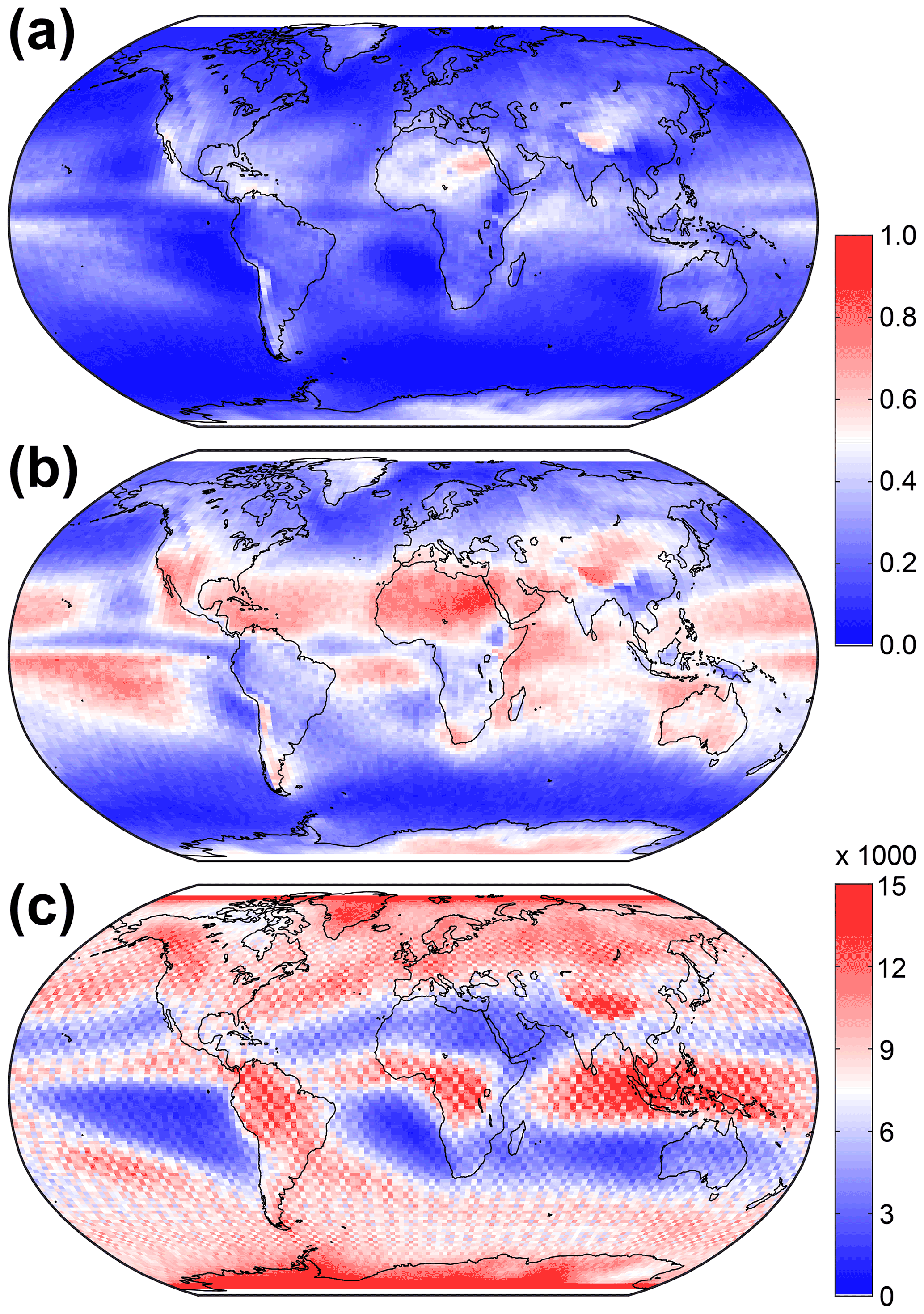
Figure 1 Global distribution of (a) the ratio of CALIPSO profiles that contain cirrus clouds in the absence of opaque low- and mid-level clouds versus all cloudy profiles, (b) the ratio of CALIPSO profiles that contain cirrus clouds in the absence of opaque low- and mid-level clouds versus all cirrus-containing cloudy profiles, and (c) the number of cirrus-containing cloudy profiles per grid box.

Differences between day and night are summarized in Fig. 2. The differences are likely related to the combined effect of diurnal variability and variations in detection sensitivity. The increased detection sensitivity during the night (related to the absence of background noise from scattered sunlight) generally leads to an increase in the number of cirrus-containing cloudy profiles south of about 55^∘ N, while the opposite is the case at higher latitudes (not shown). Nevertheless, the general patterns of cirrus occurrence for CALIPSO observations during day and night do not differ from those in Fig. 1a.

The seasonal variation of the occurrence of isolated cirrus clouds is presented in Fig. 3. The region with the highest occurrence rate of isolated cirrus clouds is northern Africa during boreal winter. Other regions of pronounced seasonal variation are the western coast of North America, Chile, the southern tip of Africa, the Arabian Peninsula, the Indian Ocean and the Indian subcontinent, Tibet and western China, the maritime continent, and the equatorial Pacific Ocean. In contrast to these regions, seasonal variations at the poles are the result of the effect of polar night and day. This can also be seen from comparing Figs. 1 and 2.

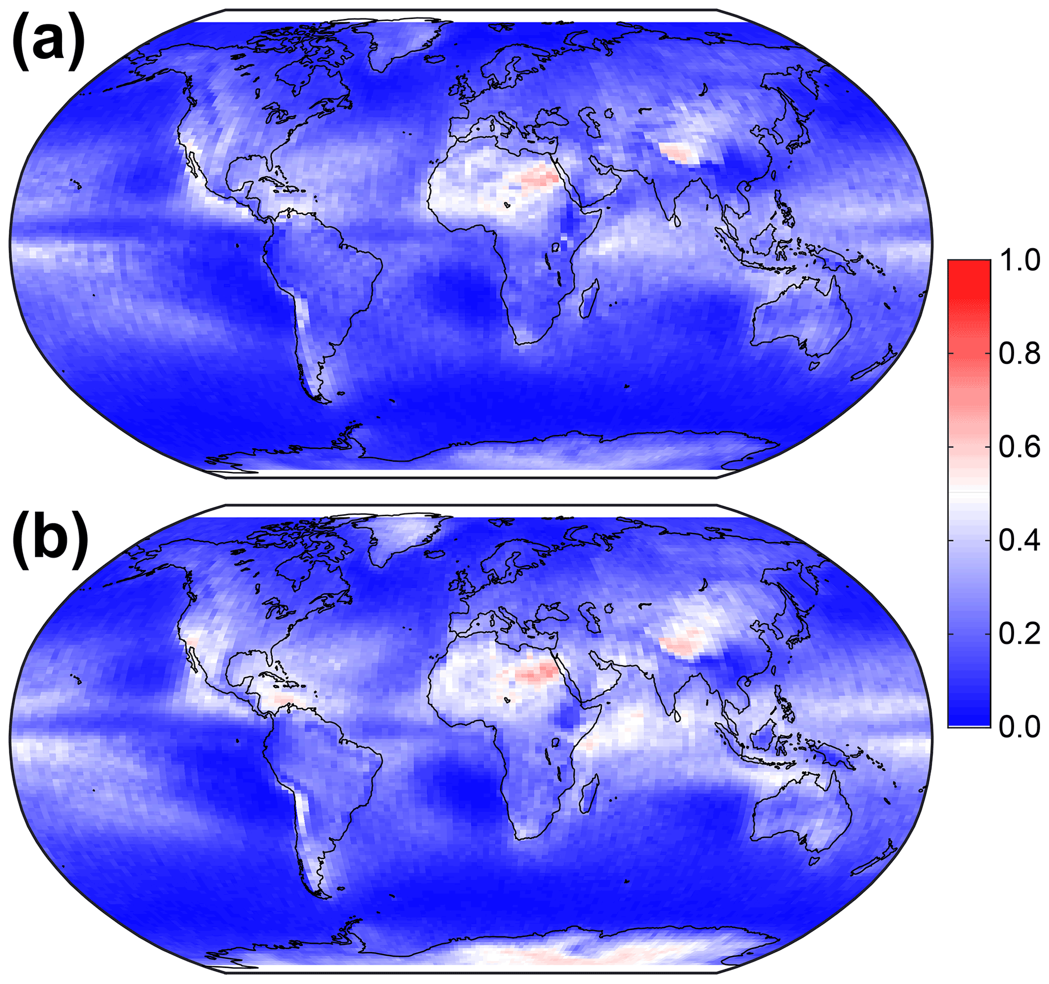
Figure 2 Same as Fig. 1a but separated according to CALIPSO observations during (a) day and (b) night.

3.2 Mid-level clouds

Occurrence rates of transparent mid-level clouds that would be detectable with a ground-based lidar from 15 years of CALIPSO data are presented in Fig. 4. The land regions with the highest fraction of CALIPSO profiles that contain transparent altocumulus clouds without low-level clouds below are the Greenland ice sheet, eastern Antarctica, the western flanks of the Rocky Mountains and Andes, western Australia, southern Africa and the Horn of Africa, large parts of the Middle East, and the area around the Himalayas. Figure 4b and c reveal that cloudy profiles containing transparent altocumulus are dominant over the continents and the equatorial oceans. A similar finding is presented in Bourgeois et al. (2016). In contrast, transparent altocumulus generally occurs less frequently over mid-latitude oceans and the stratocumulus decks to the west of the continents, though aircraft measurements have shown that the occurrence rate of thin mid-level clouds is non-negligible in these regions (Adebiyi et al., 2020).

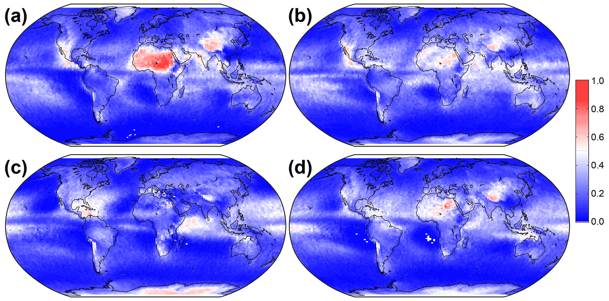
Figure 3 Same as Fig. 1a but for the 3-month periods (a) DJF, (b) MAM, (c) JJA, and (d) SON.

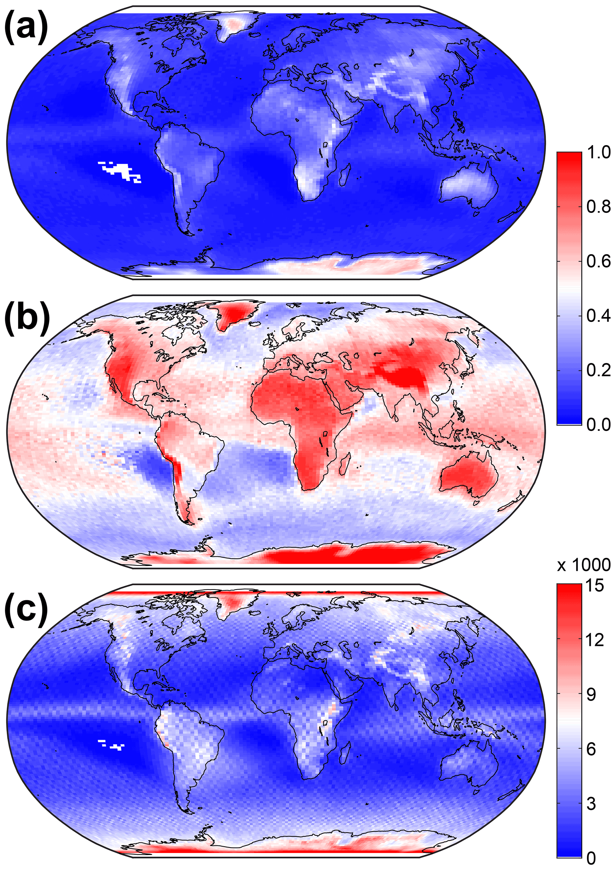
Figure 4 Global distribution of (a) the ratio of CALIPSO profiles that contain transparent altocumulus in the absence of opaque low-level clouds versus all cloudy profiles, (b) the ratio of CALIPSO profiles that contain transparent altocumulus in the absence of opaque low-level clouds versus all cloudy profiles that contain this cloud type, and (c) the number of cloudy profiles per grid box that contain transparent altocumulus.

The day–night contrast for altocumulus clouds in Fig. 5 is more pronounced than the one for isolated cirrus in Fig. 2 with a larger occurrence rate of continental transparent altocumulus clouds without low-level clouds underneath during daytime. This is particularly visible over western North America, southern and eastern Africa, eastern Antarctica, and western Australia. A slight increase in the occurrence rate is found over the equatorial oceans during the night, again likely as a result of increased detection sensitivity in the absence of the solar background. The occurrence frequency is lowest over the regions of dense stratocumulus decks to the west of the continents.

Figure 6 reveals that some regions show a considerable change in the occurrence frequency of transparent altocumulus over the year. This seasonal variation would need to be considered in the choice of location for ground-based lidar observations of mid-level clouds and in the interpretation of the collected data. For instance, ground-based lidar measurements of transparent altocumulus clouds located in northern Africa, the Middle East, or at the western coast of North America are likely to give the best yield in observations during summer, while the occurrence frequency of those clouds is considerably lower during other seasons. In contrast, the opposite is found for eastern Africa. Occurrence frequencies are relatively constant over the southern part of Africa, the Atacama region, Greenland, western Australia, and central Asia.

Figure 5 Same as Fig. 4a but separated according to CALIPSO observations during (a) day and (b) night.

Figure 6 Same as Fig. 4a but for the 3-month periods (a) DJF, (b) MAM, (c) JJA, and (d) SON.

3.3 Diurnal variability

An extensive comparison of the findings from observations with the CATS and CALIPSO lidars is provided in the Appendix. Here, the capability of CATS to cover the diurnal variability in cloudiness in the latitude band from 51^∘ S to 51^∘ N (Noel et al., 2018) is used to evaluate the representativeness of the CALIPSO lidar observations at 01:30 and 13:30 local time for drawing conclusions regarding the most suitable regions for observing mid-level and high clouds with ground-based lidar instruments. A comparison of the occurrence of high- and mid-level clouds in CALIPSO observations that cover just the CATS time period versus the 15 full years considered in Figs. 1–6 reveals no change in the observed patterns (not shown). We hence conclude that the findings of this section can be generalized to CALIPSO observations that do not fall within the time during which CATS has been active.

Figure 7 presents the analysis of CATS observations of isolated ice clouds over its full period of operation from March 2015 to October 2017. Though compiled with a coarser resolution, the occurrence-frequency map in Fig. 7a can be compared directly to the CALIPSO observations in Fig. 1a. Data from both instruments give a very similar global distribution of isolated cirrus clouds with clear maxima of occurrence over northern Africa and the Tibetan Plateau. Therefore, it is reasonable to make use of both time series for a more comprehensive analysis of the best locations for observing mid-level and high clouds with ground-based lidar.

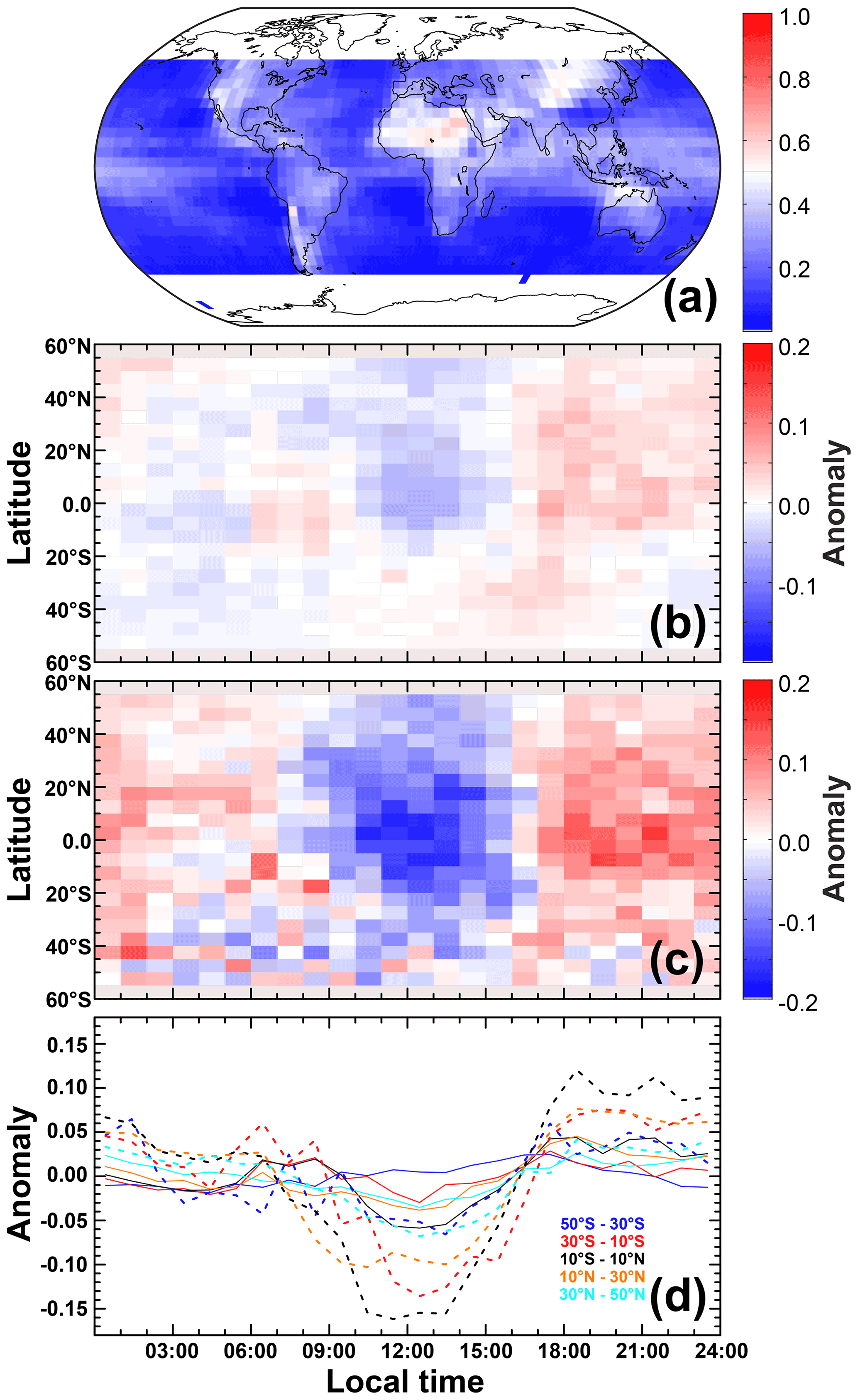
Figure 7 Occurrence rate of isolated ice clouds in CATS observations between March 2015 and October 2017 as (a) global distribution, (b) and (c) anomaly in the diurnal variation of the zonal distribution over all surfaces and land only, and (d) anomaly in the diurnal variation of the zonal average in five latitude bands: 50–30^∘ S (blue), 30–10^∘ S (red), 10^∘ S–10^∘ N (black), 10–30^∘ N (orange), and 30–50^∘ N (light blue) over all surfaces (solid) and land only (dashed). The anomaly is calculated as the difference between hourly values and the daily mean value.

The anomaly in the diurnal variation of the zonal mean occurrence rate of isolated ice clouds over all surfaces in Fig. 7b reveals that noontime measurements in the Northern Hemisphere show lower values than the daily average of CATS observations, while the opposite is the case for evening measurements. A much smaller variation from the daily average is found in the first 6 to 9 h of a day. A similar picture is found when looking at zonal mean values for different seasons (not shown). The diurnal variation in zonal bands of 20^∘ is shown in Fig. 7d. Over all surfaces, measurements in the tropics from 30^∘ S to 30^∘ N show the largest anomaly at noon and in the evening. Smaller variations are found at latitudes larger than 30^∘. All zonal bands show mean values varying around zero until 06:00 local time. Fig. 7c shows that the diurnal variation is intensified when considering only data over land, which are the areas where a ground-based lidar would be placed. In that case, a stronger negative anomaly is found around noon compared to the data over all surfaces in Fig. 7b, while a positive anomaly extends from 18:00 to 06:00 local time, though weakening after midnight. This is corroborated by the zonal means over land in Fig. 7d, which also reveal the smallest anomaly during the morning hours. From this investigation of diurnal variation and the magnitude of the anomaly during day and night, it can be concluded that CALIPSO nighttime observations at 01:30 local time might be more representative for an objective assessment of the ideal regions for observing mid-level and high clouds with ground-based lidar instruments compared to daytime observations at 13:30 local time.

The results of an analogous investigation for transparent altocumulus clouds are presented in Fig. 8. Again, the distribution of isolated altocumulus clouds from CATS observations resembles that derived from the CALIPSO time series in Fig. 4a. However, the smaller volume of the CATS data set in combination with the coarser resolution of the spatial gridding leads to a weaker contrast in altocumulus occurrence in Fig. 8a compared to the CALIPSO data in Fig. 4a. The anomaly in the diurnal variation of the zonal mean occurrence rate of isolated altocumulus is much weaker than for cirrus for observations over all surfaces as well as land only. In fact, the anomaly is negligible when considering all surfaces (Fig. 8b and d). Considering only data over land shows a weak positive anomaly around noon and an even weaker negative anomaly between 18:00 and 06:00 local time (Fig. 8c). Hence, CALIPSO observations at 01:30 local time should be representative for the better part of a day.

Figure 8 Occurrence rate of isolated mid-level clouds in CATS observations between March 2015 and October 2017 as (a) global distribution, (b) and (c) anomaly in the diurnal variation of the zonal distribution over all surfaces and land only, and (d) anomaly in the diurnal variation of the zonal average in five latitude bands: 50–30^∘ S (blue), 30–10^∘ S (red), 10^∘ S–10^∘ N (black), 10–30^∘ N (orange), and 30–50^∘ N (light blue) over all surfaces (solid) and land only (dashed). The anomaly is calculated as the difference between hourly values and the daily mean value.

3.4 Placing a ground-based lidar for observations of high and mid-level clouds

The findings of this study are summarized in Fig. 9. Additional maps with higher temporal resolution as a reference for short-term instrument deployment are provided in Figs. A5–A8. The combination of (i) the ratio of CALIPSO profiles containing either cirrus clouds in the absence of opaque low- and mid-level clouds or transparent altocumulus in the absence of low-level clouds versus all cloudy profiles (Figs. 1a and 4a) with (ii) the normalized number of such CALIPSO profiles per grid box (Figs. 1c and 4c) is used to identify those land regions where measurements with a ground-based lidar are most likely to yield the highest possible observation rate for studying mid-level and high clouds.

Unsurprisingly, cirrus clouds are best observed in the tropics with particularly suitable conditions for ground-based lidar measurements at the northern coast of South America, equatorial Africa, the southern tip of the Indian subcontinent, and the maritime continent. Cirrus observations with lidar in these regions have been performed, for instance, in Niger (Protat et al., 2010), in southern India (Pandit et al., 2015), at the Maldives (Seifert et al., 2007), and at Nauru (Comstock et al., 2002). Further favourable regions are the Tibetan Plateau (Dai et al., 2019; He et al., 2013) and western China, western North America (Sassen and Campbell, 2001; Sassen and Benson, 2001), Florida and the Caribbean (Haarig et al., 2016), the Atacama region, the southern tip of South America (Barja Gonzalez et al., 2020), the Amazon rainforest (Gouveia et al., 2017), Antarctica (Alexander and Klekociuk, 2021), and Greenland (Lacour et al., 2018), where semi-transparent clouds were found to potentially enhance ice sheet melting (Bennartz et al., 2013; Solomon et al., 2017). Less ideal conditions are met over Europe (Giannakaki et al., 2007; Kienast-Sjögren et al., 2016) and most of Asia. The worst regions are the Canadian Arctic, the northern parts of Europe and Asia, the Middle East, southern Africa, and most of Australia. Nevertheless, studies have been published based on measurements in those regions as well (e.g. Platt, 1973; Protat et al., 2010).

Figure 9 Overview of the best regions for placing a ground-based lidar for observing (a) high and (b) mid-level clouds derived from multiplying the data in Figs. 1a and 4a by the normalized number of profiles per grid box, i.e. Fig. 1c divided by 33 955 and Fig. 4c by 27 469, respectively. The colours refer to the factors for meeting suitable conditions for ground-based lidar observations of the two cloud types. For cirrus clouds, the colours mark the ranges 0.0000 to 0.0399 (white), 0.0400 to 0.0799 (light blue), 0.0800 to 0.1199 (light red), and >0.1200 (red). The corresponding ranges for altocumulus clouds are 0.0000 to 0.0249, 0.0250 to 0.0499, 0.0500 to 0.0749, and >0.0750.

The preferential regions for observing mid-level clouds with ground-based lidar are shown in Fig. 9b. These turn out to be more confined compared to the ones for cirrus in Fig. 9a. The regions that stick out are the Greenland Plateau and Antarctica (Del Guasta et al., 1993), where the topography is too high to have low-level clouds as an obstacle for lidar measurements. At low and mid latitudes, advantageous observational conditions prevail on the western flanks of the Rocky (Sassen, 2002) and Andes mountain ranges (Kanitz et al., 2011; Jimenez et al., 2020), over the Amazon, in western Australia (Protat et al., 2011), in southern and eastern Africa, in the Gulf region, on the fringe of the Tibetan Plateau, and in central Asia. The regions indicated in Fig. 9b mark those for which a ground-based lidar is likely to give the best return rate in terms of observing altocumulus clouds. This is particularly important for short-term deployments such as field experiments which typically extend over a period of a few weeks to months. Alternatively, long-term measurements are the best option for collecting a volume of data that is sufficient to allow for identifying specific case studies as well as for enabling a statistical analysis of the observed altocumulus clouds – even in regions that are not emphasized in Fig. 9b, such as central Europe (Ansmann et al., 2005; Seifert et al., 2010; Schmidt et al., 2015).

Figures A5–A8 provide seasonally and monthly resolved displays of the data in Fig. 9. The figures reflect the annual variation of observational conditions for consideration when planning the deployment of lidar instruments for observing mid-level or high clouds during dedicated field experiments or shorter-term measurement campaigns.

4 Summary and conclusions

Fifteen years of measurements from the polar-orbiting CALIPSO lidar have been used in combination with 32 months of measurements from the CATS lidar aboard the International Space Station between March 2015 and October 2017 to investigate the global distribution of cloud scenarios that support observations of mid- and high-level clouds with ground-based lidar instruments. The CALIPSO cloud mask was used to select profiles in which

1. cirrus clouds are observed in the absence of low-level clouds and opaque altocumulus underneath and

2. transparent altocumulus is observed in the absence of low-level clouds underneath

as an analogue for conditions under which a ground-based lidar could be used for unperturbed observations of high- and mid-level clouds, respectively.

The fixed CALIPSO overpass times at 01:30 and 13:30 local time inhibit an assessment of the diurnal variation in cloudiness. Hence, observations with the CATS lidar have been used to investigate the representativeness of the CALIPSO cloud sampling. While the CATS data set flags water and ice clouds, additional screening is needed to identify cloud types such as altocumulus and cirrus as provided in the CALIPSO data set. Scenarios that are comparable to the ones selected from the CALIPSO observations have been compiled by screening the CATS data set for the occurrence of cloud ice and for the location of cloud base and top heights.

The analysis of the data sets from the two spaceborne lidars shows a remarkable resemblance in the regional and vertical distribution of isolated cirrus and altocumulus clouds despite the different approaches to extracting the corresponding information from the two data sets. The diurnal variation of cloud occurrence from the CATS data set leads to the conclusion that CALIPSO observations at 01:30 local time are representative for the better part of the day, while the period of the largest anomaly is covered by the overpass at 13:30 local time. Generally, diurnal anomalies in cloud occurrence are (i) stronger over land compared to over all surfaces and (ii) stronger for isolated cirrus clouds compared to isolated altocumulus clouds. The ratio of occurrence of the two cloud types versus all cloudy profiles per grid box in combination with the absolute number of profiles in a corresponding grid box is used to identify those regions for which a ground-based lidar is likely to encounter the best balance between the occurrence of the desired cloud types and the prevalence of favourable conditions to actually observe these clouds, i.e. the absence of strongly light-attenuating clouds below the target cloud.

This information is particularly vital in planning deployment of lidar instruments in the framework of field experiments or measurement campaigns. Such deployments generally last between a few weeks and several months, and their success relies strongly on finding atmospheric conditions that meet the desired research objectives to allow for addressing related science questions. From the approach used in this study, it is found that the best regions for lidar measurements of cirrus clouds are the tropics, the Tibetan Plateau, the western part of North America, the Atacama region, the southern tip of South America, Greenland, Antarctica, and parts of western Europe. For the observation of altocumulus clouds, a ground-based lidar is best placed on Greenland, Antarctica, the western flank of the Andes and Rockies, the Amazon, central Asia, Siberia, western Australia, or the southern half of Africa. The seasonally and monthly resolved view of advantageous conditions for observing mid-level and high clouds with ground-based lidar reveals a strong annual variation for some of the regions identified above that should be considered in the planning of shorter-term lidar deployments. Finally, it should be emphasized that the regions identified here provide the best gain of a lidar deployment. However, this advantage for short-term deployments can be compensated for by increasing the length of a lidar operating at a certain site, as this increases the likelihood of meeting the desired atmospheric conditions for observing a targeted cloud type.

Appendix A: Comparability of CALIPSO and CATS observations of the fraction of high- and mid-level clouds

The consistency of observations with the CALIPSO and CATS lidars is investigated for the time period from March 2015 to October 2017, i.e. the period of CATS operation. For this, CATS observations of ice and mid-level clouds collected in a time period of ±1 h around the CALIPSO observations at 01:30 and 13:30 local time are used to derive cloud fraction (i) in grid boxes of 5^∘ by 5^∘, (ii) as latitudinal and longitudinal averages, and (iii) in the form of height profiles for comparison to CALIPSO observations. Note that the temporal constraint leads to a much lower number of CATS profiles compared to the CALIPSO observations and thus more noise in the CATS data.

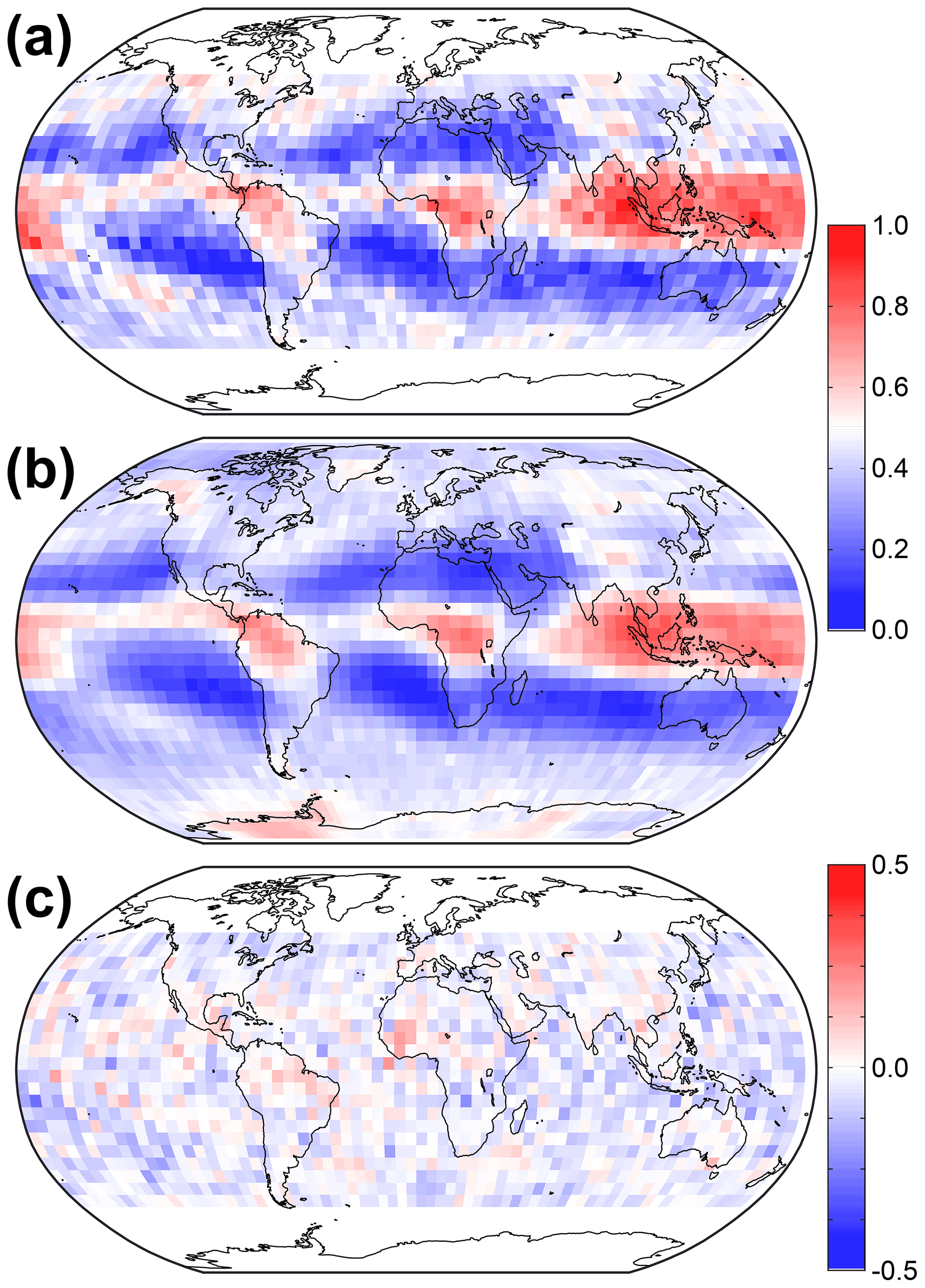
Figure A1 Global distribution of the fraction of cirrus clouds in observations with the (a) CATS and (b) CALIPSO lidars and (c) difference between CALIPSO and CATS for the time period from March 2015 to October 2017. Only CATS data within ±1 h around the fixed CALIPSO overpass times are considered.

Figure A2 (a) Latitudinal distribution and (b) height profiles of the cloud fractions of isolated cirrus as seen by CALIPSO (black) and of isolated ice clouds as seen by CALIPSO (red) and CATS (blue) for the time period from March 2015 to October 2017.

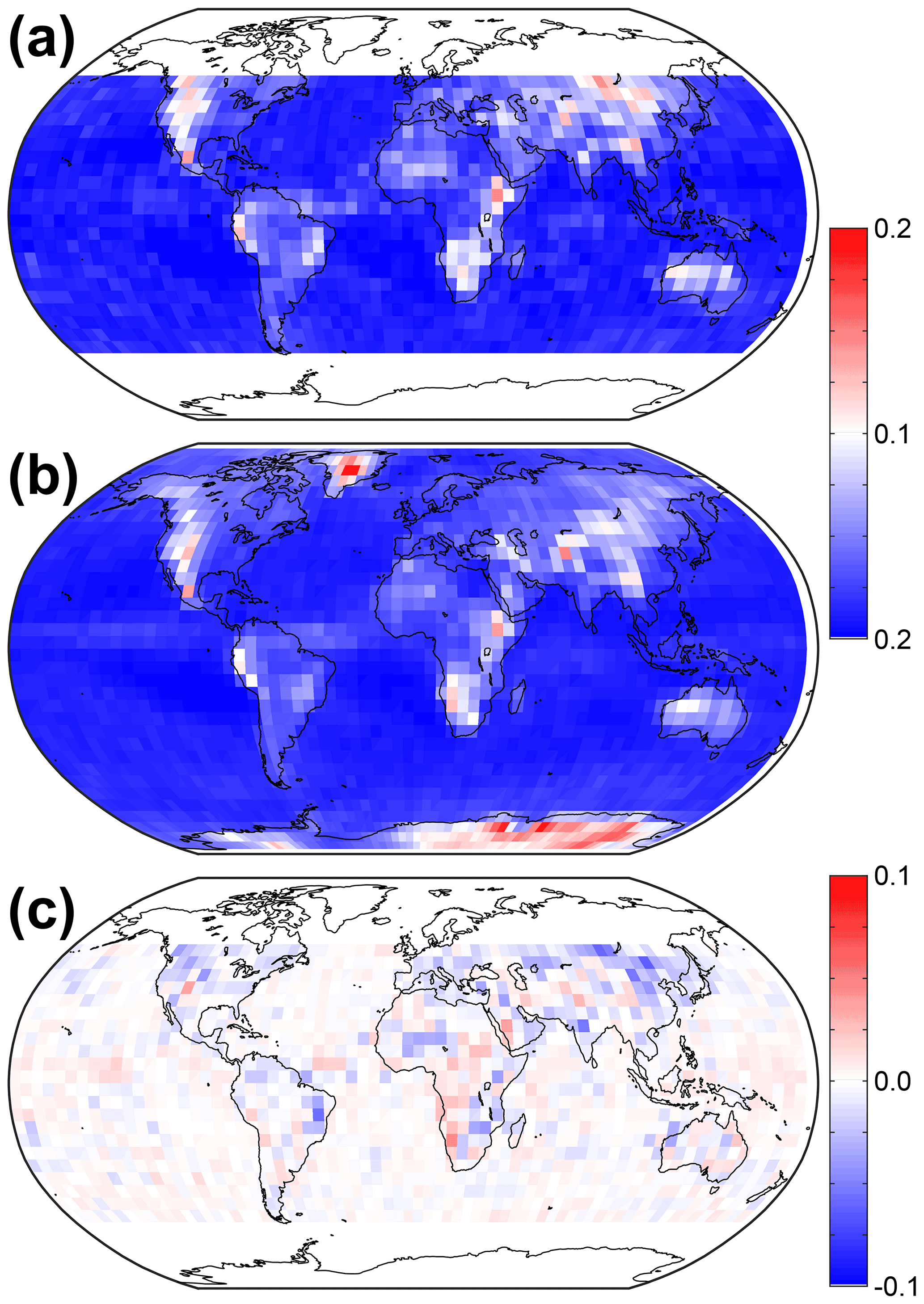
Figure A3 Global distribution of the fraction of mid-level clouds in observations with the (a) CATS and (b) CALIPSO lidars and (c) difference between CALIPSO and CATS for the time period from March 2015 to October 2017. Only CATS data within ±1 h around the fixed CALIPSO overpass times are considered.

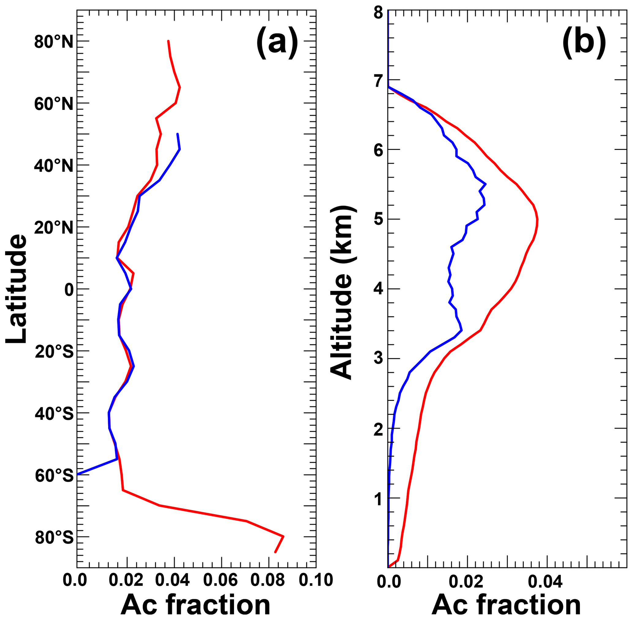
Figure A4 (a) Latitudinal distribution and (b) height profiles of the altocumulus cloud fraction as seen by CALIPSO (red) and CATS (blue) for the time period from March 2015 to October 2017.

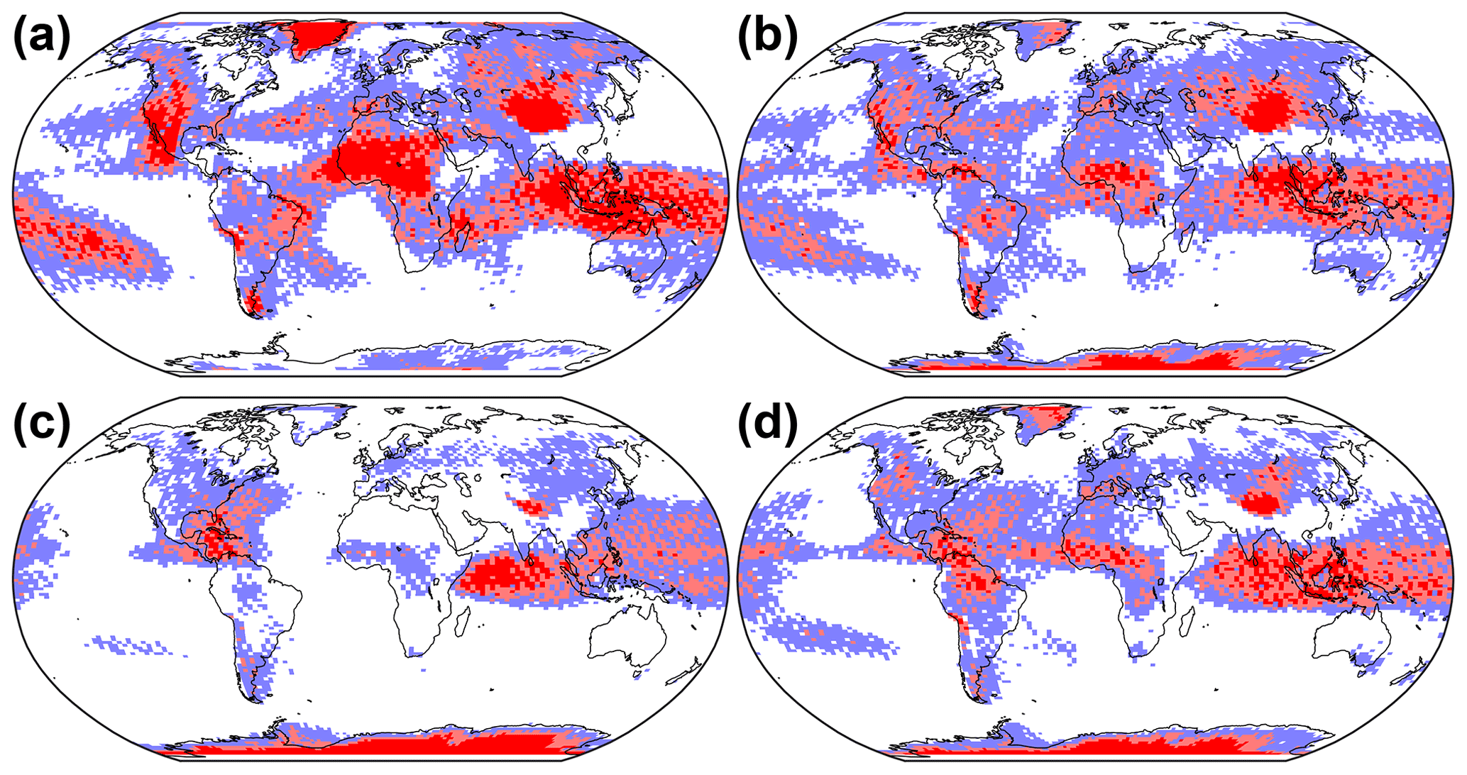
Figure A5 Same as Fig. 9a but for the 3-month periods (a) DJF, (b) MAM, (c) JJA, and (d) SON.

A1 Cirrus clouds

Figure A1 compares the spatial distribution of the occurrence frequency of cirrus clouds as seen by CALIPSO and CATS. Both data sets agree in their main features, i.e. maxima of ice-cloud fraction over the tropics, regions of low ice-cloud fraction in bands around 30 and 30^∘ N, and an increase in ice-cloud fraction towards higher latitudes from there. This agreement is confirmed when considering latitudinal and longitudinal averages (not shown). The CATS and CALIPSO data sets agree in the magnitude of latitudinally averaged ice-cloud fraction with the largest deviation of about 0.05 in the band at 25^∘ S, an effect that might be resulting from the noise in the CATS data. The longitudinally averaged ice-cloud fraction shows bands with a larger deviation between the two data sets (from 150 to 120^∘ W and from 50^∘ W to 50^∘ E) as well as bands for which the averages overlay almost perfectly. Again, noise induced from the decreased number of grid boxes for deriving the values is likely to affect the comparison. Both instruments reveal an almost identical vertical distribution of ice clouds (not shown) within the latitude band ±5^∘, where they feature a roughly similar sampling rate. This agreement corroborates the findings of Sellitto et al. (2020).

Figure A1 refers to all ice clouds. For a fair comparison with the CALIPSO data in Fig. 1a, i.e. clouds that are (i) flagged as cirrus and (ii) are the only cloud type in the profile, the CATS data set has been screened for what is referred to here as isolated cirrus clouds. The cloud subtype classification is not available in the CATS data set. However, when only ice clouds are present in a profile (i.e. they are not the top of a larger system or part of a mixed-phase system) and these clouds are not flagged as opaque, they are most likely to be cirrus. The CALIPSO Atmospheric_Volume_Description variable and the CATS Percent_Opacity_Fore_FOV variable are used to select clouds that are neither opaque nor fully attenuated.

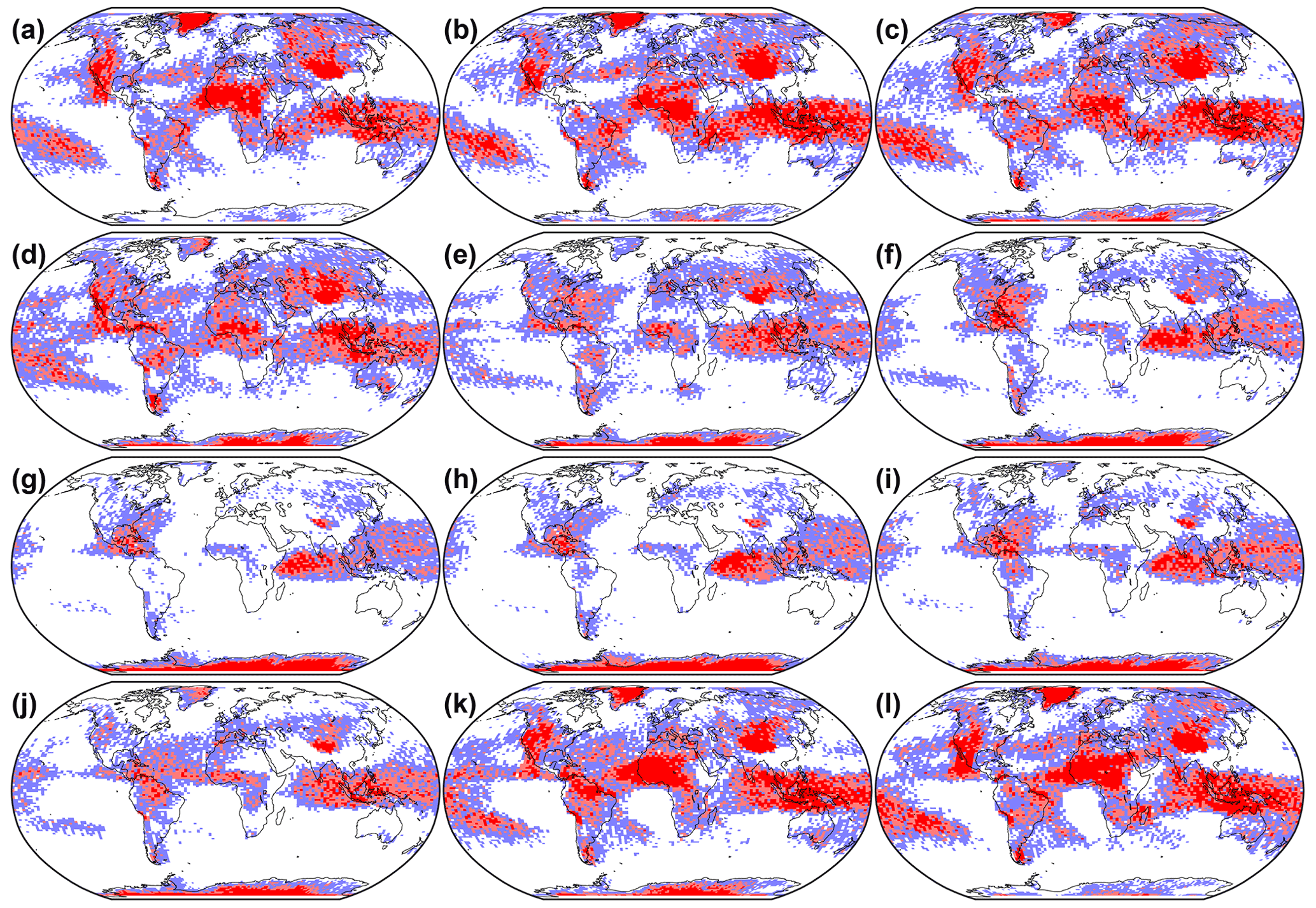
Figure A6 Same as Fig. 9a but for individual months: (a) January, (b) February, (c) March, (d) April, (e) May, (f) June, (g) July, (h) August, (i) September, (j) October, (k) November, and (l) December.

Figure A7 Same as Fig. 9b but for the 3-month periods (a) DJF, (b) MAM, (c) JJA, and (d) SON.

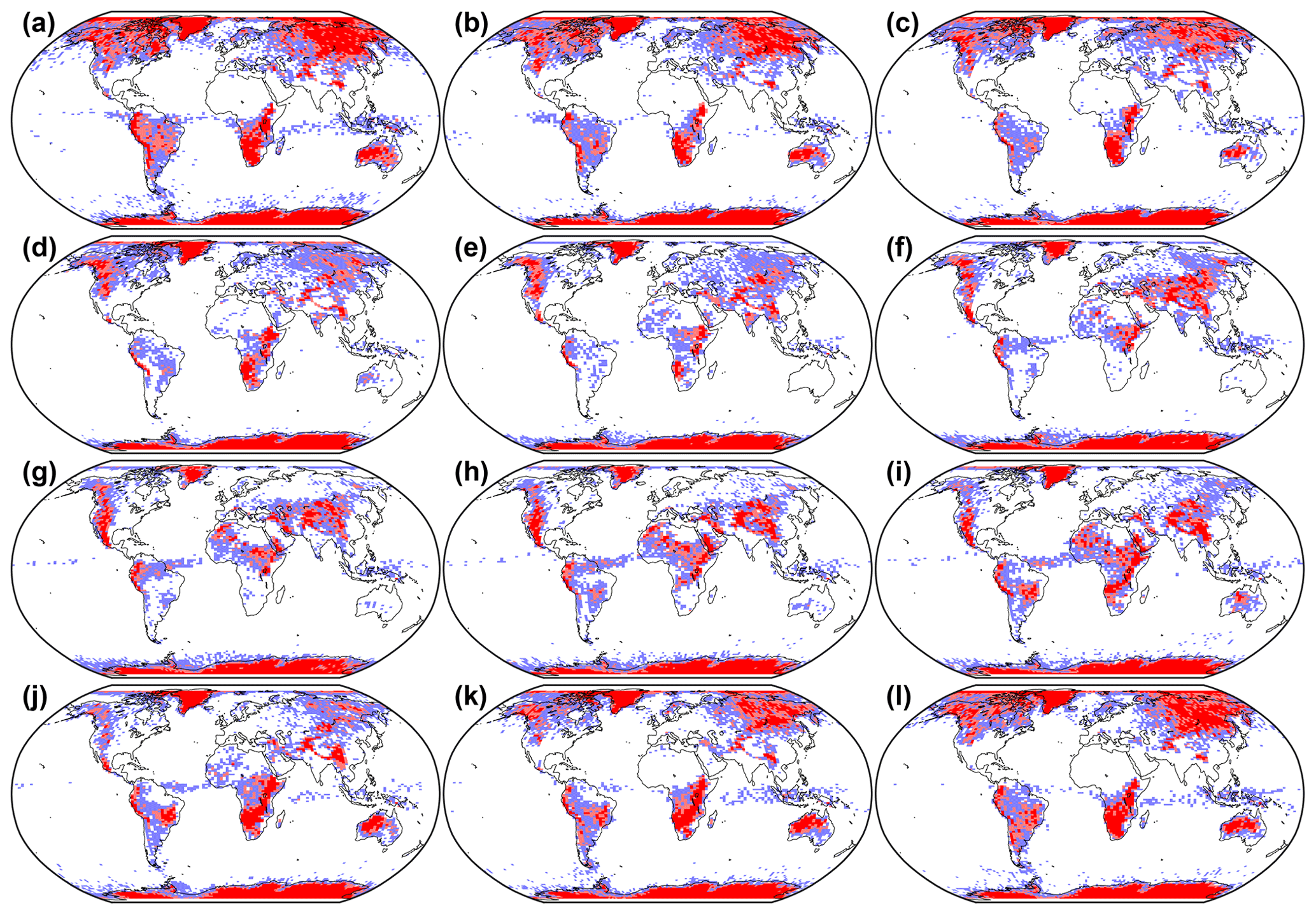
Figure A8 Same as Fig. 9b but for individual months: (a) January, (b) February, (c) March, (d) April, (e) May, (f) June, (g) July, (h) August, (i) September, (j) October, (k) November, and (l) December.

Figure A2 shows that the vertical profile and the zonal average of the fraction of isolated ice clouds as seen by CATS match those seen by CALIPSO very closely. About 75 % to 95 % of isolated ice clouds between 7.5 and 17.5 km height are categorized as cirrus. Moreover, 88 % of profiles containing isolated ice clouds in CALIPSO data between 51^∘ S and 51^∘ N are categorized as cirrus (92 % for 30^∘ S to 30^∘ N). This fraction decreases towards higher latitudes beyond the area of CATS data coverage between 51^∘ S and 51^∘ N. The findings in Fig. A2 suggest that the majority of isolated ice clouds in non-opaque CATS profiles are equivalent to isolated cirrus in CALIPSO data. In addition, cloud-fraction retrievals for isolated ice clouds in non-opaque profiles give comparable results when using data from the CALIPSO and CATS instruments. As a consequence, the investigation of the diurnal variability of ice clouds considers CATS profiles that contain isolated, non-opaque ice clouds and assumes that these profiles are equivalent to CALIPSO profiles that contain isolated cirrus clouds.

A2 Mid-level clouds

Figure A3 compares the spatial distribution of the occurrence frequency of transparent mid-level clouds as seen by CALIPSO and CATS during the CATS period of operation. Overall, the occurrence frequency is much lower than for ice clouds in Fig. A1. In addition, transparent altocumulus is observed primarily over land. Both time series resolve comparable regions of high altocumulus occurrence frequency over southern and eastern Africa, the Middle East, central Asia, western Australia, the Amazon, coastal Peru, and to the west of the Rocky Mountains. Discernible differences are restricted to northern Africa, central Asia, and eastern Australia – all regions where CATS finds a slightly higher altocumulus occurrence frequency than CALIPSO.

Figure A4a shows that the small differences in Fig. A3 do not lead to a large deviation in the zonal mean altocumulus fraction. The only exception is visible around 40^∘ N, where the higher altocumulus occurrence frequency over western North America and central Asia in CATS observations compared to CALIPSO leads to a higher zonal mean in the CATS data set. The vertical distribution of altocumulus fraction in Fig. A4b shows that both instruments place the target clouds within the same height range with a maximum at around 5 km height but a larger altocumulus fraction in the CALIPSO data set compared to the one derived from CATS measurements. As in the case of cirrus in Fig. A4b, different absolute maxima in the profiles of cloud fraction from CALIPSO and CATS are most likely the result of slight differences in how these cloud types are inferred from the measurements of the two instruments.

Appendix B: Seasonal and monthly variation

The information in Fig. 9 might not be specific enough to consider where to put a ground-based lidar for observing high- and mid-level clouds for a shorter-term field experiment. Seasonally and monthly resolved displays of the data in Fig. 9 are therefore presented in Figs. A5–A8 to resolve the annual variation in the advantageous conditions for observing altocumulus and cirrus clouds with ground-based lidar.