High-resolution satellite-based cloud detection for the analysis of land surface effects on boundary layer clouds

The observation of boundary layer clouds with high-resolution satellite data can provide comprehensive insights into spatiotemporal patterns of land-surface-driven modification of cloud occurrence, such as the diurnal variation of the occurrence of fog holes and cloud enhancements attributed to the impact of the urban heat island. High-resolution satellite-based cloud-masking approaches are often based on locally optimised thresholds that can be affected by the local surface reflectance, and they therefore introduce spatial biases in the detected cloud cover. In this study, geostationary satellite observations are used to develop and validate two high-resolution cloud-masking approaches for the region of Paris to show and improve applicability for analyses of urban effects on clouds. Firstly, the Local Empirical Cloud Detection Approach (LECDA) uses an optimised threshold to separate the distribution of visible reflectances into cloudy and clear sky for each individual pixel accounting for its locally specific brightness. Secondly, the Regional Empirical Cloud Detection Approach (RECDA) uses visible reflectance thresholds that are independent of surface reflection at the observed location. Validation against in-situ cloud fractions reveals that both approaches perform similarly, with a probability of detection (POD) of 0.77 and 0.69 for LECDA and RECDA, respectively. Results show that with the application of RECDA a decrease of cloud cover during typical fog or low-stratus conditions over the urban area of Paris for the month of November is likely a result of urban effects on cloud dissipation. While LECDA is representative for the widespread usage of locally optimised approaches, comparison against RECDA reveals that the cloud masks obtained from LECDA result in regional biases of ±5 % that are most likely caused by the differences in surface reflectance in and around the urban areas of Paris. This makes the regional approach, RECDA, a more appropriate choice for the high-resolution satellite-based analysis of cloud cover modifications over different surface types and the interpretation of locally induced cloud processes. Further, this approach is potentially transferable to other regions and temporal scales for analysing long-term natural and anthropogenic impacts of land cover changes on clouds.

1 Introduction

The detection of continental boundary layer clouds based on satellite data has a long tradition and is essential for the analysis of the various ways that clouds interact with the land surface from the climate scale to the microscale. Different land cover types, such as vegetation and urban surfaces, exhibit distinct physical surface properties that influence the latent and sensible heat fluxes between the surface and the boundary layer and thus cloud development and spatial patterns (Shepherd, 2005; Collier, 2006; Varentsov et al., 2018).

Frequently, satellite-based analyses of the impact of land surface characteristics on boundary layer clouds are based on comparisons of cloud fraction and its spatial anomalies with respect to different land cover types (Teuling et al., 2017; Theeuwes et al., 2019; Pauli et al., 2022). Characteristic modifications of spatial patterns of cloudiness can emerge over urban areas. For example, an afternoon cloud cover enhancement has been found over Paris during summer (Theeuwes et al., 2019), whereas fog frequencies have been observed to be lower over the urban areas of the Gangetic Plain during winter (Gautam and Singh, 2018). In this context, the urban heat island effect has been found to be a main driver of the boundary layer cloud enhancement over Paris (Theeuwes et al., 2019). In many cases, the mechanisms by which the land surface characteristics interact with the spatial patterns in cloudiness are not well understood (Zhong et al., 2017; Fan et al., 2016; Liang et al., 2018; Shepherd, 2005; Collier, 2006; Han et al., 2014).

Satellite data are ideally suited to map patterns of cloudiness and facilitate the analysis of land surface–atmosphere interactions at various scales. The High Resolution Visible (HRV) channel of the Spinning Enhanced Visible and Infrared Imager (SEVIRI) sensor onboard Meteosat Second Generation (MSG) is particularly useful in this context due to its high temporal (∼ 15 min) and spatial resolutions (1 km at nadir) (Klüser et al., 2008; Deneke and Roebeling, 2010; Derrien et al., 2010; Henken et al., 2011). High-resolution cloud masks enable the detection and analyses of modifications to spatial patterns of cloudiness induced by small-scale (effective spatial resolution of HRV in this region ∼ 2 km) features. While the higher spatial resolution is a clear advantage of the HRV channel, cloud detection from the single spectral HRV channel is hampered by missing multi-spectral information that is available at coarser resolutions (e.g. 3 km at nadir for SEVIRI). This is shown by the large number of cloud detection algorithms that are based on multi-spectral thresholding tests to separate clear sky from different cloud types (Ackerman et al., 1998; Rossow and Garder, 1993; Saunders and Kriebel, 1988; Stowe et al., 1999; Di Vittorio and Emery, 2002; Chen et al., 2003; Hutchison et al., 2005; Cermak, 2006; Yang et al., 2007; Bley and Deneke, 2013; Andersen and Cermak, 2018).

HRV-based cloud detection methods for deriving cloud masks are rare and challenging due to the limitation of observations from a single visible channel (Schulz et al., 2012; Nilo et al., 2018). Cloud masks obtained from a single channel are often based on histograms and seek to separate the clear-sky and cloudy components of the reflectivity distribution. The separation of the distribution is typically based on a threshold that is determined by a histogram-based minima approach in a representative data set of a specific surface type and geographic region (Minnis and Harrison, 1984; Ipe et al., 2003; Bley and Deneke, 2013; Cermak, 2006; Cermak and Bendix, 2008). For the empirical determination of the clear-sky reflectivity, the frequent occurrence of atmospheric and non-atmospheric features can be challenging, as aerosols, cloud shadows, thin cirrus clouds and fresh snow affect the retrieved reflectances (Yang et al., 2007; Ipe et al., 2003; Matthews and Rossow, 1987). In general, thresholds determined by such techniques are temporally dynamic to account for the diurnal and seasonal variations of the solar zenith angle (Yang et al., 2007) and the vegetation period (Teuling et al., 2017; Theeuwes et al., 2019). The main problem for cloud detection is the influence of the land surface signal on the clear-sky determination that can lead to severe misinterpretation of cloud occurrence over different surface types. For example, over bright surfaces a reduced contrast between clear-sky reflection and cloudy-sky reflection can lead to an under-detection of clouds (EUMETSAT, 2019). To account for location-specific differences in surface albedo and to reduce the local bias, thresholds determined over land are frequently locally optimised. Teuling et al. (2017) suggested an empirical approach that flags an observation as cloudy when reflectivity exceeds a locally (per pixel) and temporally (per hour, 10 d period) adjusted clear-sky climatological value. Such locally adjusted and empirically based thresholds have a low bias in total but are still challenged by a degradation of detection accuracy depending on the local surface brightness (Bley and Deneke, 2013). This is caused by locally optimised approaches that seek to find the optimal threshold to distinguish clouds and clear sky and thus have to deal with a surface-dependent bias (see explanation in Sects. 3.2 and 1b). For analyses of land surface impacts on clouds, however, it is crucial that the satellite-based detection of cloud occurrence over different land cover types is independent of variations in surface properties, like spectral albedo. With such an application-focused algorithm there is a great potential to further improve the understanding of cloud formation and dissipation processes with respect to regional characteristics.

In this study, two approaches to detect boundary layer clouds on the basis of SEVIRI HRV data are presented and compared for the analysis of cloud cover changes over different surface types: the locally optimised cloud detection scheme of the Local Empirical Cloud Detection Approach (LECDA) and the Regional Empirical Cloud Detection Approach (RECDA) that is more robust to regional variations in surface reflectivity. Both approaches are processed for November of a multi-year period over a large region of Paris and its surrounding area. During this month, fog occurs frequently and can be expected to be affected by the urban region of Paris (Gautam and Singh, 2018). Results are validated with measurements of a CloudNet station in the southwest of Paris.

In Sect. 2, the data used are described. The methods to derive LECDA and RECDA and their validation with in situ CloudNet data are explained in Sect. 3. Section 4 presents the results, a discussion of the comparison and the validation of the two cloud-masking approaches, and a meteorological case using RECDA. Section 5 contains the conclusions.

2 Data

2.1 SEVIRI satellite data

The main part of this study, including the generation of cloud masks, is based on the analysis of SEVIRI HRV data, which have a spatial resolution of 1 km at nadir and cover a broadband range from 0.4 to 1.1 µm. Together with the remaining three solar and eight thermal SEVIRI channels with a spatial sampling distance of 3 km at nadir, the Earth is observed in a repeat cycle of 15 min covering the full disc for the low-resolution channels and half of the full disc for the HRV channels. It must be noted that spatial resolutions of the low- and high-resolution channels are effectively lower than the given sampling distance due to the satellite viewing geometry and the fact that the reflectance field is oversampled by a factor of 1.6 (Deneke and Roebeling, 2010; Schmetz et al., 2002, MSG level 1.5 image data format description). For the detection and removal of snow and ice clouds, channel reflectances of the visible channels (0.6 and 1.6 µm) and brightness temperatures of the infrared channels (8.7, 10.8 and 12.0 µm) are used, respectively (see Sect. 3.1). In total, the time period of the data set spans the month of November from 2004 to 2019 (08:00–16:00 UTC), resulting in ∼ 14 400 time steps. The study region is the urban area of Paris and the adjacent rural areas extending from 48.0 to 49.6^∘ N and from 1.6 to 3.0^∘ E (Fig. 4b), where urban cloud modifications have already been observed and are considered relevant for the urban climate of Paris during summer (Theeuwes et al., 2019). The urban area of Paris further serves as an ideal test bed as it is surrounded by relatively homogeneous and flat terrain with altitude ranges of ∼ 200 m (see Fig. 6b). The month of November was chosen to investigate a possible reduction in fog clouds over the urban area of Paris as found in other regions during winter (Gautam and Singh, 2018). Further, with the selection of 1 month, seasonal variations of land cover, e.g. due to the vegetation period, can be neglected and long-term variability of the surface reflectance can assumed to be small.

2.2 CloudNet data

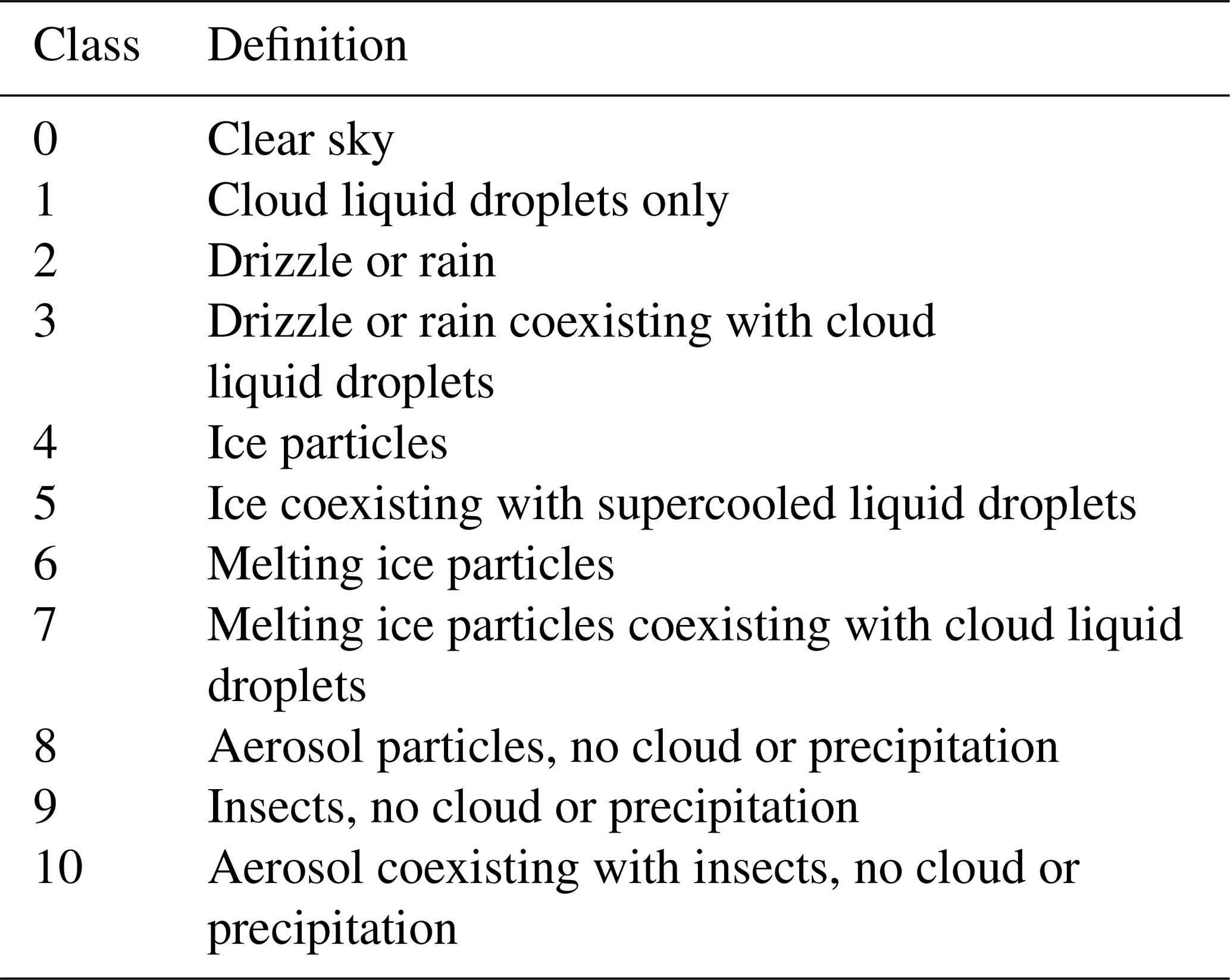
The cloud masks are validated against the calibrated CloudNet classification product (CF-1.0, level 2) for November (2015 to 2019) at Palaiseau (48.718^∘ N–2.202^∘ E) located ∼25 km to the southwest of Paris at 156 $\mathrm{m}\mathrm{a}.\mathrm{s}.\mathrm{l}.$ (Illingworth et al., 2007). The location of the CloudNet station is shown in Fig. 2. Ground-based remote sensing instrumentation, including a ceilometer, a Doppler cloud radar, a microwave radiometer from the atmospheric observatory SIRTA (Site Instrumental de Recherche par Télédétection Atmosphérique, Haeffelin et al., 2005) and model outputs of the ECMWF Integrated Forecast System (IFS), serve as input for the CloudNet target classification algorithms described in ACTRIS Deliverable WP5 D5.5 (M24). As a result, a classification into 11 classes distinguishes between ice and water clouds, precipitation, aerosols, insects, clear sky, and combinations thereof (See Table A1 in Appendix A) is obtained in a 30 s time interval and for 719 heights above sea level with a vertical resolution of 25 m (168.5–18 118.5 m).

2.3 Reanalysis data

To highlight the applicability of the novel cloud mask data set generated by the regional approach to study surface-driven modifications of fog cloud cover, ERA5 data are used to filter for atmospheric conditions under which these clouds typically occur. ERA5 hourly data on single levels from 1979 to present of the European Centre for Medium-Range Weather Forecasts (ECMWF; Hersbach et al., 2018) are averaged over the study region, and SEVIRI scenes are selected only if all of the following criteria are met: 10 m wind speed that is <3 m s⁻¹ ($U/V$ wind component), boundary layer height (BLH) that is <300 m and mean sea level pressure (MSL) that is >1020 hPa. These are boundary layer conditions that characterise and facilitate the formation of fog and low-strata cloud.

2.4 CORINE land cover

For comparisons between cloud fraction anomalies over different land cover types, CORINE land cover (CLC) level 3 data for 2012 (version 2020_20u1) at 100 m spatial resolution provided by the Copernicus Land Monitoring Service are used (European Environment Agency, EEA, 2021). The land use in 2012 only shows minor differences compared to the available land cover classifications in 2006 and 2018 and is chosen here to represent the period 2004–2019. CLC 2012 data are resampled to the HRV spatial resolution by using the most frequent land cover class within a HRV pixel (Fig. 4a). Only relevant land cover classes, including forests, continuous or discontinuous urban fabric, arable land, and pastures, are considered for a more detailed analysis.

2.5 Digital elevation model

The European Digital Elevation Model (EU-DEM; version 1.1) is used to compare changes in altitude of small-scale features of cloud fraction anomalies (Fig. 6b). The data set has a spatial resolution of 25 m and is provided by the Copernicus Land Monitoring Service (EEA, 2017; Tøttrup, 2014).

3 Methods

3.1 Snow and ice filter

The preprocessing of the HRV data includes the elimination of ice clouds and snow in order to retain only liquid and mixed clouds for the data analysis. This is done by using threshold tests on the SEVIRI channels at 0.6, 1.6, 8.7, 10.8 and 12 µm and collocating the flagged pixels with the associated HRV pixels. In this way, data that are not relevant for the analysis of urban cloud modifications are excluded from the data set.

Snow is detected by calculating the Normalised Difference Snow Index (NDSI) based on the 0.6 and 1.6 µm channels:

$$\begin{array}{}\text{(1)}& \text{NDSI}={\displaystyle \frac{r_{\mathrm{0.6}}-r_{\mathrm{1.6}}}{r_{\mathrm{0.6}}+r_{\mathrm{1.6}}}},\end{array}$$

where r_λ is the reflectance at wavelength λ (µm) (Dozier and Painter, 2004; Cermak, 2006). Tests done for specific scenes revealed a threshold of 0.3 to be suitable to detect snow. Pixels that feature an NDSI above this value are excluded from the data set. This approach has been widely and operationally applied to different satellite data, including MODIS and Sentinel-2 satellite sensors (Hall et al., 2001; Richter et al., 2012).

A second filter is applied to exclude ice clouds from the data set with a brightness temperature below 263 K in the 10.8 µm channel. To exclude potential remaining ice clouds, the difference between the 8.7 and 12 µm channels is used in a phase test to retain only liquid clouds. Ice absorbs much more strongly than liquid water between 10 and 13 µm, while both show a similar absorption pattern from 8 to 10 µm (Strabala et al., 1994; Cermak, 2006). The brightness difference should thus be smaller for ice clouds and is implemented as in Westerhuis et al. (2020) with the fog and low-stratus confidence level CL_FLS:

$$\begin{array}{}\text{(2)}& {\text{CL}}_{\mathrm{FLS}}={\displaystyle \frac{T_{\mathrm{LC}}-(T_{\mathrm{12}\mathrm{\mu }\mathrm{m}}-T_{\mathrm{8.7}\mathrm{\mu }\mathrm{m}})-T_{\mathrm{CCR}}}{-\mathrm{2}{T}_{\mathrm{CCR}}}},\end{array}$$

where T_LC = 1.8 K is the threshold for liquid clouds and T_CCR = 1 K is the cloud confidence range. Details of this approach can be found in Westerhuis et al. (2020). Pixel values with a CL_FLS below 0 are removed from the data set to retain only low-level liquid clouds.

Figure 1 (a) Conceptional distribution of a bimodal distribution of HRV pixel counts for one SZA bin and one pixel within the study region during November 2004–2019. The first and second components of the Gaussian mixture model present clear (red) and cloudy conditions (blue) with the local clear-sky reflectance CS_loc (vertical dashed black line) and a potential clear-cloud threshold T_loc (vertical black line). Clear-sky reflectance is defined as the maximum count per histogram bin (maxbin) of the CS GMM component. The histogram minimum would be a potential threshold to separate the near-Gaussian distributions of clear and cloudy pixels for this time and location. Panel (b) is the same as (a) over a bright and a dark surface with the corresponding cloud fraction (CF). Both figures are created with three randomly generated Gaussian distributions: a distribution for the cloudy conditions and two distributions for surfaces of different brightness (Sect. 3.2), showing the surface-brightness-driven shift in the threshold that leads to different estimates of cloud fraction in this artificial example.

3.2 Two approaches to delineate clouds and clear sky

3.2.1 Gaussian mixture model

Based on this preprocessed data set the Local Empirical Cloud Detection Approach and the Regional Empirical Cloud Detection Approach is proposed to delineate clouds from clear sky resulting in two different cloud masks (CMloc and CMreg). The ultimate goal of RECDA is to derive spatially unbiased cloud fraction anomalies over different land cover types, while the goal of LECDA is a pixel-by-pixel cloud detection with minimum bias.

Both approaches are relatively simple and nearly independent of other channel information. The thresholds are determined empirically based on occurrence frequencies of HRV counts in solar zenith angle (SZA) bins as shown conceptually in Fig. 1a for a single SZA bin and pixel. The first peak of the distribution presents clear-sky conditions (CS), while the second refers to cloudy (CL) conditions.

In both approaches the CS composite is obtained by applying a Gaussian mixture model (GMM) to the HRV reflectance histograms of each SZA bin and each pixel within the study region. A GMM is a probabilistic model that assumes that the data are generated from a mixture of a finite number (here this number is two: CS and CL in Fig. 1a) of Gaussian probability distributions with unknown parameters. This method is categorised as an unsupervised learning algorithm that works in a similar way as the distance-based k-means cluster method. Instead of a distance-based model, the algorithm finds the clusters based on Gaussian probability distributions. Based on the expectation minimisation algorithm, conditional expectations of the complete log likelihood are calculated, and estimates (mean and covariance) are updated iteratively until convergence to a local optimum is reached (Jain et al., 2000). While this method is limited to near-Gaussian distributions of a representative data set (excluding high SZA bins, where a bimodal distribution of clear sky and cloud is not always existent) and a sufficient amount of data, it has great potential beyond the simple usage of a binary cloud mask as it provides probabilities (Sci-kit learn implementation, Pedregosa et al., 2011).

In this setup, the GMM characteristics of the CS component are exploited to dynamically (pixel-based per SZA bin) derive thresholds. In the following, the computation of a local T_loc (1) and a regional threshold T_reg (2) is described based on the maximum bin count and standard deviation of the GMM CS component.

3.2.2 Local Empirical Cloud Detection Approach (LECDA)

In this approach a local HRV threshold T_loc is obtained based on the CS probability distribution (first GMM component) per SZA slot (five SZA bins 67–77; >1000 data points) and per pixel as follows. First, the local clear-sky reflectance CS_loc (Fig. 1a), which is determined by the reflectance value using the maximum count per histogram bin (maxbin) with a bin width of 0.5 within the mean ±2σ range of the CS GMM maxbin approach, is preferred over taking the mean of the first GMM component as it is representative for CS. Second, T_loc is computed as the sum of CS_loc (per pixel) and the regional median of all local 3σ of the CS GMM component. The regional median is chosen to increase the robustness of the derived T_loc against a sub-optimal local fit of the GMMs due to atmospheric noise, such as aerosols. In general, this method is assumed to be less contaminated by the effect of cloud shadows, aerosols and thin cirrus clouds compared to similar clear-sky minimum approaches as it is based on the maximum bin count of the GMM clear-sky distribution (Bley and Deneke, 2013; EUMETSAT, 2019). However, the impact of these atmospheric features on the results cannot be entirely excluded and may distort the clear-sky reflectance.

$$\begin{array}{}\text{(3)}& {\displaystyle }{\mathrm{\text{CS}}}_{\mathrm{loc}}=\text{maxbin}\in [\text{mean}+\mathrm{2}{\mathit{\sigma }}_{\mathrm{CSGMM}},\text{mean}-\mathrm{2}{\mathit{\sigma }}_{\mathrm{CSGMM}}]\text{(4)}& {\displaystyle }{T}_{\mathrm{loc}}={\text{CS}}_{\mathrm{loc}}+{\text{MED}}_{\mathrm{reg}}\left(\mathrm{3}{\mathit{\sigma }}_{\mathrm{CSGMM}}\right)\end{array}$$

Thresholds obtained by LECDA as in Eq. (4) are used in, for example, Teuling et al. (2017) and present a straightforward method to approximate the “real” cloud fraction. In their study a similar local cloud mask approach is proposed, where a constant threshold (10 counts) is added to an empirically determined clear-sky value for a given pixel based on a cumulative distribution function of reflectivity measurements. However, such locally optimised approaches including LECDA are dependent on variations in surface albedo due to different land cover types as a constant value is added to the clear-sky reflectance shown in Fig. 2 and Eq. (4). A brighter clear-sky surface pixel within the urban area of Paris will shift the clear-sky distribution to higher reflectance and thus clear-cloud thresholds assuming a constant cloud distribution as schematically illustrated using synthetic data in Fig. 1b. Due to the dynamic threshold method (pixel-based per SZA bin) that seeks to distinguish bright clear-sky surface pixels from clouds in a narrower bimodal distribution, a higher threshold is set in the case of brighter pixels compared to darker pixels. As a direct consequence, the application of LECDA for the retrieval of cloud fraction can potentially result in an underestimation of clouds over bright surfaces when compared to clouds over dark surfaces (see the legend of Fig. 1b for an example) given a constant cloud distribution over both surfaces.

As comparability of cloud detection over different surface albedos is not assured by LECDA, and to address the potentially resulting bias, RECDA is developed to use one regional threshold for all pixels of the study area (Eq. 5).

3.2.3 Regional Empirical Cloud Detection Approach (RECDA)

In this approach T_reg is obtained by setting the maximum of all T_loc as a “static” threshold that is applied to all pixels in the study area per SZA.

$$\begin{array}{}\text{(5)}& T_{\mathrm{reg}}=\text{max}\left(T_{\mathrm{loc}}\right)\end{array}$$

RECDA is thought to result in a slight underestimation of clouds for all pixels as it sets the reflectance threshold to a higher reflectance value. The advantage compared to the LECDA is that RECDA is independent of different surface albedo values (Fig. 2) and is therefore better suited to the comparison of regional cloud fraction anomalies over different land surfaces. The influence of the surface signal during the prevalence of thin liquid clouds may affect the cloud distribution but is assumed to be minor compared to the dependence of LECDA on the surface signal (see Sect. 4.2).

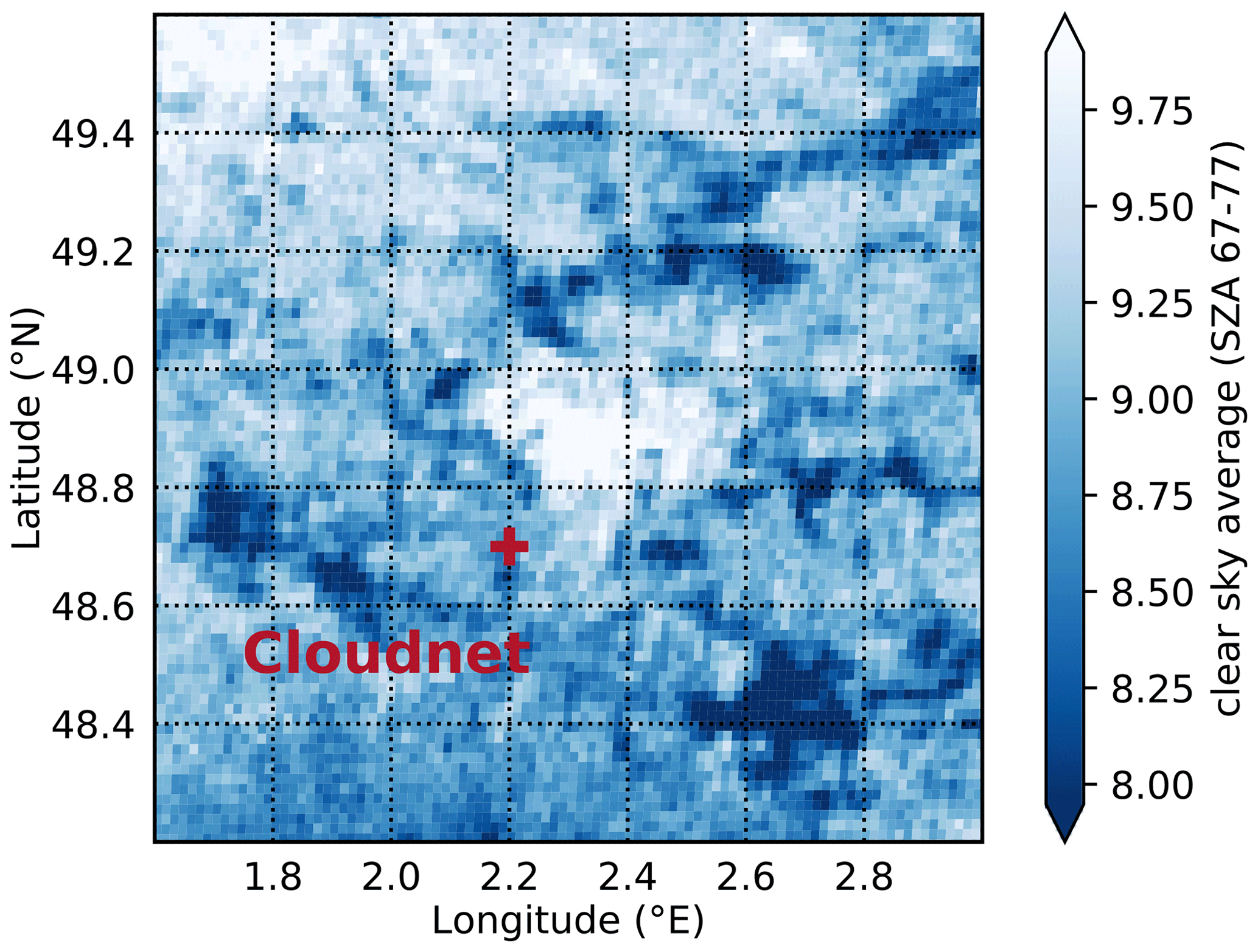
Figure 2 Average (SZA bins 67–77) of clear-sky reflectance CS_loc obtained by Eq. (3). The location of the CloudNet station at Palaiseau used for validation is marked in red.

3.3 Local evaluation using CloudNet data

CloudNet data are used to evaluate and compare the local performance of both approaches. In order to aggregate the CloudNet data to the temporal resolution of SEVIRI (15 min interval), CloudNet cloud fraction is calculated for each time step based on a 1 h time window centred around the corresponding SEVIRI time slot. This time window was chosen according to findings by Deneke et al. (2009) that compared SEVIRI satellite pixel (3 km×6 km) with ground-based radiometer measurements. A correction factor of 11 min was added to the SEVIRI time slot to match the SEVIRI nominal time with the actual scanning time over the validation site. Its calculation is based on the time SEVIRI needs per revolution (0.6 s) to scan one line (three image lines at a time) from south to north, accounting for the acquisition start at 81^∘ S, the spreading distance of the ground resolution in the S–N direction and the number of scan lines (MSG level 1.5 image data format description). The W–E scan time of 30 ms is neglected. Details of the computation for the low-resolution channels can be found in Kim et al. (2020) with the same nominal time as the HRV channel.

All CloudNet target classifications per time window are considered relevant for the validation of the cloud mask. To create a CloudNet cloud fraction as ground truth, classes 1 to 7 are assigned as cloudy, while 0 and 8 to 10 are assigned as clear sky (see Table A1; Veefkind et al., 2016). If one of the 719 vertical target layers at one specific time step is classified as cloud, the observation at this time step is flagged as cloud. If the resulting CloudNet cloud fraction of the defined time window is above 0.5, the CloudNet flag of the corresponding SEVIRI time is assigned as cloud (1) and is otherwise assigned as clear sky (0). This selected time window will ensure that only persistent cloud observations are matched with the SEVIRI cloud mask.

The temporally aggregated CloudNet cloud mask is compared to a spatial aggregate of 3 × 3 HRV cloud mask pixels ($\sim \mathrm{3}\mathrm{km}\times \mathrm{6}\mathrm{km}$) centred around the CloudNet validation station. Due to the oblique viewing angle of SEVIRI, a parallax correction is required, resulting in a horizontally displacement of the pixel matrix surrounding the validation station by ∼ 2.6 km (two pixels) to the north (Greuell and Roebeling, 2009; Schutgens and Roebeling, 2009). If more than four out of the nine matrix pixels are cloudy, the matrix is aggregated to one value assigned as cloud (1) and is otherwise assigned as clear sky (0). This matrix approach was chosen in order to fully capture clouds traversing the validation sight and to reduce the effect of cloud inhomogeneity and partial cloud cover (Deneke et al., 2005).

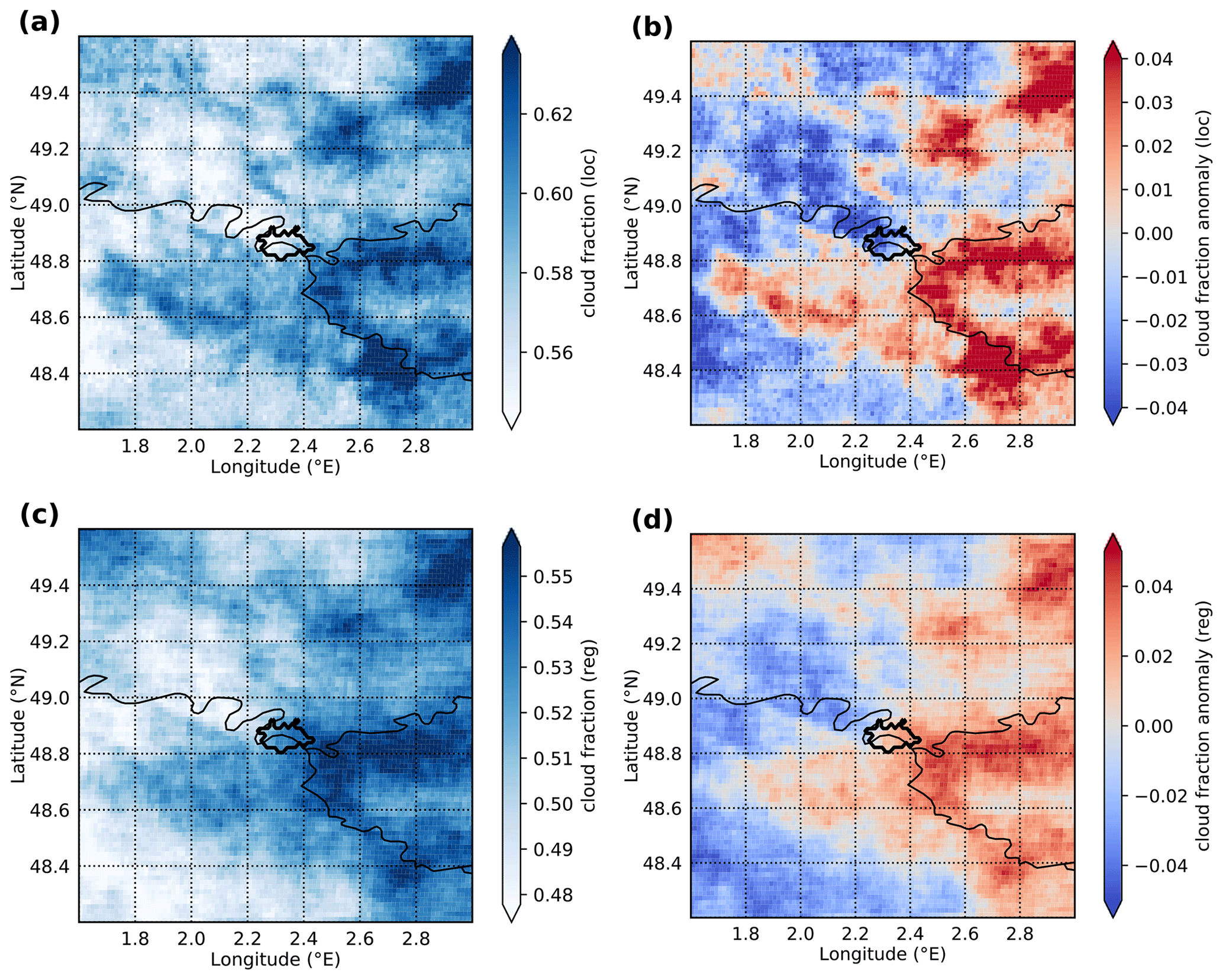
Figure 3 Cloud fraction CF_loc and CF_reg (a, c) and their spatial anomalies CF_locanomaly and CF_reganomaly (b, d) over the region of interest for the month of November during the years 2004–2019. Larger rivers are visualised as black lines, and the continuous urban area of Paris is shown as a black contour.

4 Results and discussion

4.1 Comparison of the two cloud-masking approaches

Figure 3 shows cloud fractions and their regional anomalies from the local and regional empirical cloud detection approaches, CFloc and CFreg. CFloc and CFreg are defined as the number of cloudy pixels divided by the total number of pixels, and their regional anomaly (CF_locanomaly, CF_reganomaly) is defined as the difference between the cloud fraction of the pixel and the average cloud fraction of the region. The spatial patterns of CF_loc and CF_reg in Fig. 3a and c are similar and show a high cloud fraction and hence a positive anomaly in Fig. 3b and d in a triangular shape east and northeast of Paris where the river valleys of the Oise, Marne and Seine are located. While CF_loc shows generally higher cloud fractions and a slightly larger anomaly range with more small-scale features, CF_reg spatial patterns are less distinct and more smooth. As expected, due to the algorithm differences (see Sect. 3.2), CF_reg is lower (on average by 7 %) than CF_loc.

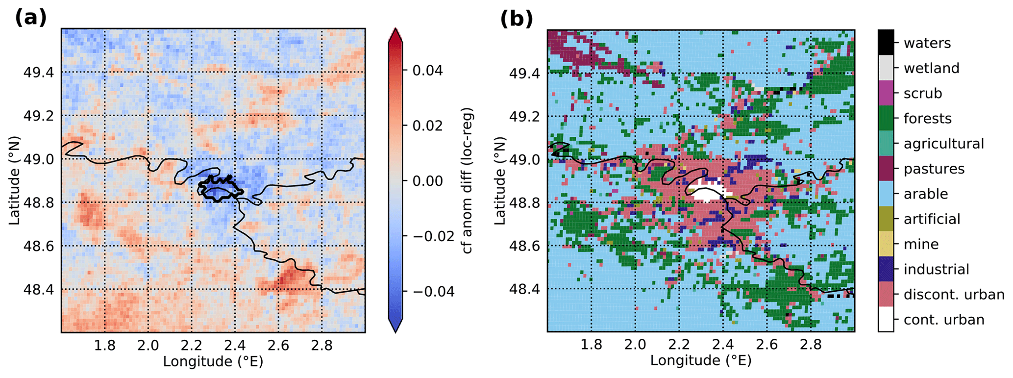
Figure 4 (a) Difference between cloud fraction anomalies (CF_locanomaly−CF_reganomaly) from local and regional empirical cloud detection approaches. (b) Main CORINE land cover classes L2 and L3 for the year 2012. Larger rivers are visualised as black lines.

Figure 5 (a) Difference between cloud fraction anomalies (LECDA–RECDA) and clear-sky reflectance (average of SZA bins 67–77). Bright colours represent a higher probability density of the data points using Gaussian kernels. (b) Difference between cloud fraction anomalies (CF_locanomaly−CF_reganomaly) from local and regional empirical cloud detection approaches grouped by five main CORINE land cover types: forest, continuous urban fabric, discontinuous urban fabric, arable land and pastures. The median and mean of each class are presented as horizontal orange lines and black dots, respectively. Whiskers are equal to 1.5 times the interquartile range beyond the first and third quartiles. Outliers are shown as black circles.

Differences between the two cloud-masking approaches are shown in Fig. 4a by mapping the difference of their respective cloud fraction anomaly patterns (CF_locanomaly-CF_reganomaly). The differences are most prominent over the urban region of Paris and over forests (cf. Fig. 4b) and are clearly connected with the clear-sky reflectance of these different land cover types (cf. Fig. 2). The comparison of the respective cloud fraction anomalies reveals a relative underestimation of CF_loc by more than 4 % over the relatively bright urban area of Paris, while it leads to a relative overestimation of clouds over some of the relatively dark forest areas. The general dependence of LECDA on the surface reflectance is shown in Fig. 5a, where the difference between LECDA and RECDA is a function of clear0sky surface reflectance. A total of 75 % of the variability in the difference between RECDA and LECDA can be explained by the surface reflectance. It is assumed that the dependence on the surface reflectance is mostly attributed to LECDA, while a small portion may be attributed to RECDA in conditions of thin liquid clouds. Grouping these cloud fraction anomaly differences by land cover types confirms these observations and shows that the relative biases over the continuous urban area of Paris exceed the biases over the forest region (Fig. 5b). The pasture land cover type present in the northwestern parts of the region also shows a relative underestimation of the local approach; however, local differences from the surrounding land cover types are not clearly visible. The contribution of land cover variability within a HRV pixel (see resampling of land cover classes, Sect. 2.4) is expected to have a marginal influence on the cloud statistics.

4.2 Analysis of cloud patterns in typical fog conditions

Patterns of cloud clearings over urban areas are mostly expected in conditions of fog or low-stratus cloud (Gautam and Singh, 2018). In order to test the application of CM_reg to study spatial patterns of urban cloud modification, the derived cloud mask is filtered for specific boundary layer conditions using the ERA5 reanalysis data (cf. Sect. 2.3). Cloud fraction anomaly patterns constrained by these meteorological conditions show small-scale features that can be clearly associated with surface characteristics (Fig. 6). Notable is the distinct relative decrease of presumed fog and low-stratus cloud fraction directly over the centre of Paris and extending to its western edges on the order of ∼ 10 % relative to the regional average CF. This spatial pattern is usually associated with the dissipation of fog or low-stratus cloud by depletion of liquid water at the surface or the lifting of the cloud base (Wærsted et al., 2019; Williams et al., 2015; Underwood and Hansen, 2008; Haeffelin et al., 2005). This negative cloud fraction anomaly is likely a signal of the occurrences of fog holes (Gautam and Singh, 2018) over the urban centre of Paris. It is interesting to note that the negative anomaly extends to the west of the city, suggesting that in the high-pressure situations considered here winds may be predominating from easterly directions. The effect of wind direction on the cloud fraction anomaly is considered minor due the focus on conditions with low wind speeds only.

Positive cloud fraction anomalies show clear links to topography, especially over river valleys where fog is naturally favoured (Bendix, 2002). This is visible in the northeast (Oise), the northwest (Epte, Avelon, Thérain), and east and southeast (Marne, Seine) of the study area. The high-resolution cloud fraction anomaly map thus highlights the ability of the regional approach to detect small-scale cloud patterns that can be linked to land cover characteristics and the topography.

For a systematic assessment of the land surface influences on spatial cloud fraction anomalies in the study region, cloud fraction anomalies are grouped by land cover types in Fig. 7. The land cover class “continuous urban” shows an average negative cloud fraction anomaly of 6 % that can be interpreted as a lower bound of the magnitude of the city's effect on fog occurrence, as Paris is located in a river valley and should thus have favourable conditions for fog formation. Over pastures an increase by 4 % is notable; however, this is likely linked to the location of the pastures in the Avelon river valley in the NW of the study area. Smaller anomalies of the remaining land cover classes are partly explained by the combined influence of land cover type, terrain height and the dynamic of the fog hole evolution itself. Discerning the way that this cloud pattern is linked to the urban heat island of Paris, the land surface characteristics and any further meteorological variables will require further analysis beyond the scope of this paper.

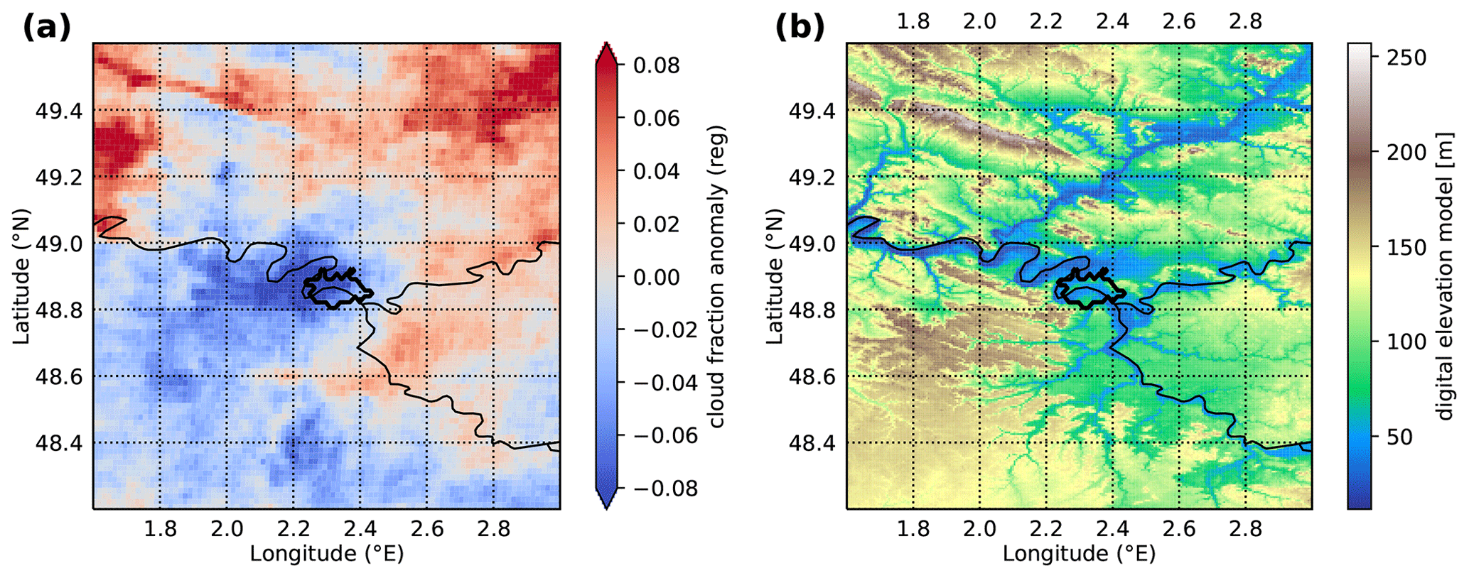
Figure 6 (a) Cloud fraction CF_reg anomaly (difference between the cloud fraction of the pixel and the average cloud fraction of the region) from the Regional Empirical Cloud Detection Approach constrained by the following meteorological conditions: low wind speed (<3 m s⁻¹), low BLH (<300 m) and high MSL (>1020 hPa). (b) European Digital Elevation Model with a spatial resolution of 25 m. The Seine river is visualised as a black line.

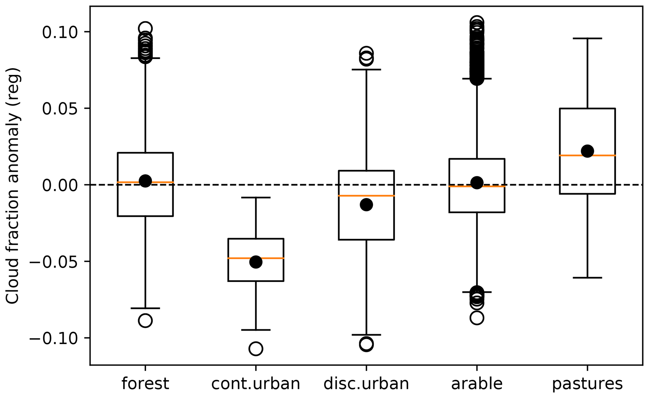
Figure 7 Cloud fraction CF_reg anomaly from the Regional Empirical Cloud Detection Approach constrained by meteorological conditions (Fig. 6) and grouped by five main CORINE land cover types: forest, continuous urban fabric, discontinuous urban fabric, arable land and pastures. Details are the same as in Fig. 5.

4.3 Validation with ground-based cloud fraction

The validation of the two cloud masks CM_loc and CM_reg with respect to the CloudNet data seeks to compare both approaches with ground truth data using standard measures of performance. However, it is not intended to prove the better applicability of one over another for the analysis of land surface effects on boundary layer clouds, as shown in Figs. 4a and 5a.

In Table 1 it is shown that both approaches perform similarly in terms of overall quality but achieve this with very different performance characteristics. In general, CM_loc outperforms CM_reg with a probability of detection (POD) of 0.77 compared to 0.69. However, the false alarm ratio (FAR) of 0.0 for CM_reg falls below that for CM_loc of 0.04. These results are expected as T_loc is generally lower than T_reg (except where $T_{\mathrm{loc}}=max\left(T_{\mathrm{loc}}\right)$), leading to a general underestimation of clouds in CM_reg with the benefit of reducing false alarms. It is notable that a main difference in validating both approaches originates from the definition of a more cloud-conservative threshold vs. a more clear-conservative threshold.

Table 1 CloudNet validation results for the cloud masks using the local (CM_loc) and the regional (CM_reg) threshold. Validation measurements used are as follows: probability of detection (POD), false alarm ratio (FAR), percentage correct (PC), critical success index (CSI), bias score (BS) and Heidke skill score (HSS).

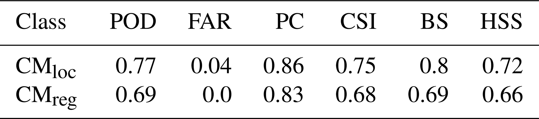
The CloudNet data validate both approaches over a location with a surface reflectance of 8.65 (see Fig. 2) that is close to the scene average of 8.96. It is expected that the validation of the local and regional approach will give the same or nearly identical results over the bright surfaces of the city, while over darker forest regions the local approach is likely to have a much higher POD, with little influence on the FAR.

For assessing the general performance of both approaches (CM_reg and CM_loc) in the context of various thresholds, POD and FAR are computed along the range of HRV values and exemplary for different SZA (Fig. 8). The resulting pseudo-ROC (receiver operating characteristic) curves can be used to determine the ideal threshold for cloud detection, which typically can be found in the upper-left-hand corner with a minimal FAR and a maximal POD. The main outcome is that CM_reg for the SZA bins 67(–69) and 69(–71) is close to being an optimal tradeoff, achieving a low FAR while losing only little detection skill (POD) when compared to CM_loc and alternative HRV thresholds. The proposed regional approach, however, shows a lower POD compared to the local approach that can be attributed to the general cloud underestimation that is true for all the different surface reflectances equally. Further, for the application suggested in this study the ROC cannot provide a measure to evaluate the performance of LECDA compared to RECDA as done in Sect. 4.2.

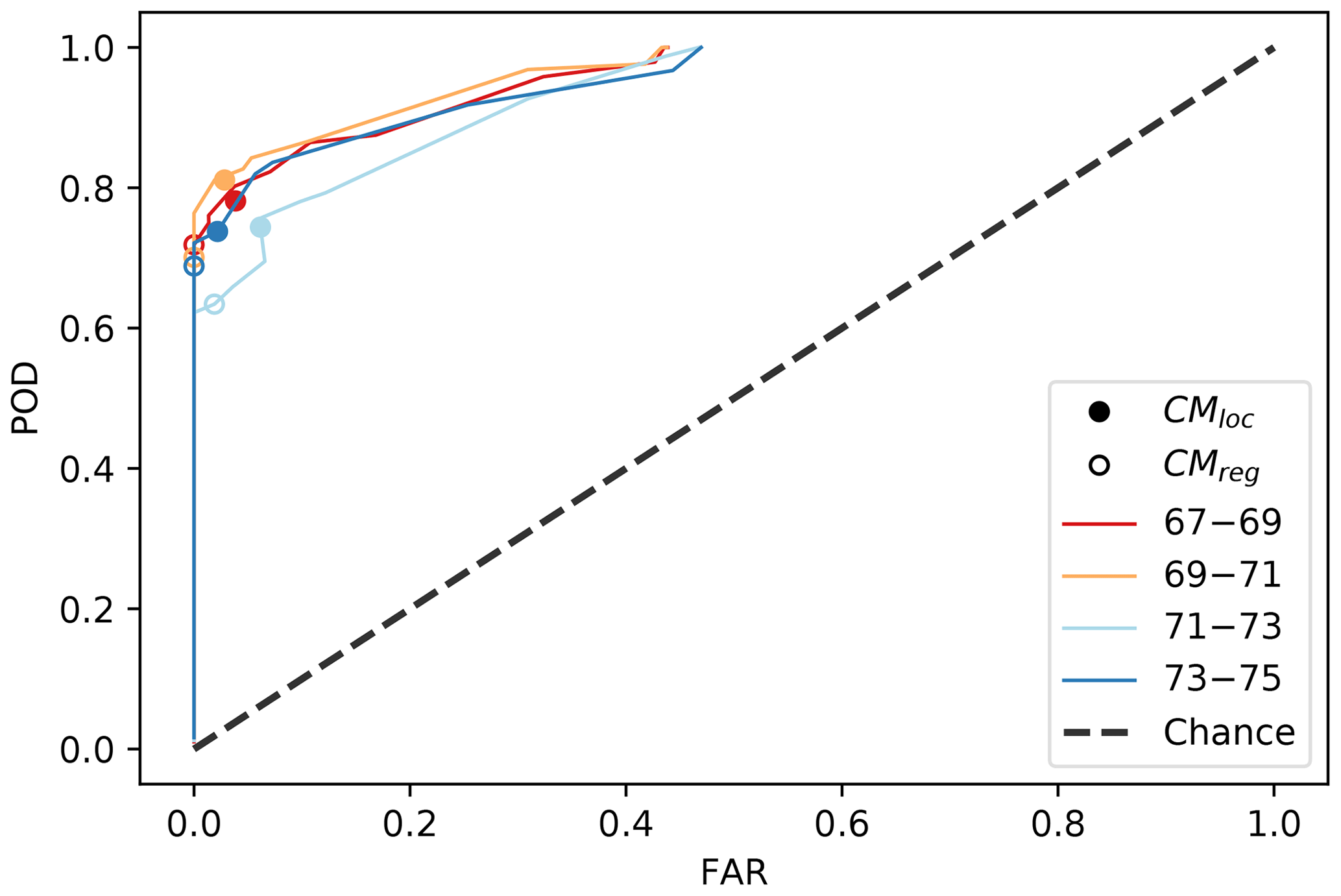
Figure 8 Relationship of POD and FAR for local and regional cloud masks (CM_loc and CM_reg; filled and transparent circles) and for a range of different HRV threshold values and four solar zenith angle (SZA) bins (coloured lines). HRV threshold values increase from the top to the bottom of the plot, i.e. from HRV minimum to HRV maximum per SZA. The pseudo-ROC curve shows the best performance of the HRV threshold values used for cloud masking in the upper-left corner, while accuracy decreases towards the dashed diagonal line.

The ground-based validation of the satellite-retrieved cloud masks is difficult as differences can be due to the specific measurement methods, including the different scales and the way cloud net data are aggregated to match the satellite data (cf. Greuell and Roebeling, 2009).

The performance of RECDA may vary depending on the location-specific characteristics of the land cover type, the satellite viewing geometry and the domain size. It is assumed that the performance of RECDA (similar to LECDA) will decrease in cases where the bimodal distribution broadens and flattens due to the effect of aerosols, thin liquid clouds, subpixel clouds or cloud edges contributing to the overlap area. It is expected that the presence of thin liquid clouds can lead to a surface-dependent bias in RECDA that is assumed to be minor compared to the influence of the surface signal in LECDA. Based on this study we can recommend RECDA for the proposed application and suggested domain size with a clear-sky reflectance between 8 % and 10 % (see Fig. 2). RECDA will not provide reliable results over regions with clear-sky reflectances varying between 8 % and 50 %, e.g. agricultural and desert regions. In addition, the gradual approximation of cloud and clear-sky reflectance in the morning and evening twilight contributes to the flattening of the distribution curve and will degrade the ability of both algorithms to separate clouds and clear sky. The SZA dependence of the clear-sky reflection is known by other cloud mask algorithms as well, e.g. EUMETSAT (2019).

5 Conclusions

This study presents and compares the applicability of two empirical cloud-masking approaches based on the single HRV channel of MSG SEVIRI for the high-resolution analysis of land surface effects on boundary layer clouds. The performance of the cloud mask based on the regional approach RECDA is compared to the local approach LECDA with respect to the influence of the underlying surface. Both cloud mask approaches and obtained cloud fractions are analysed over a $\sim \mathrm{150}\mathrm{km}\times \mathrm{150}\mathrm{km}$ region centred on Paris, where holes in fog and low-stratus cloud are expected.

It is shown that cloud masks obtained from LECDA result in a relative underestimation of cloud occurrence over the bright urban surface of Paris (up to 5 %), while cloud occurrence is overestimated in relative terms over dark surfaces, e.g. forests (up to 5 %), when compared to RECDA. This leads to the conclusion that studies using such locally optimised approaches have to be attentive when associating different land surface classes to cloud occurrence.

The application of the regional approach RECDA to compute cloud masks in contrast to a pixel-based surface-dependent threshold is shown to be advantageous as local biases due to differences of surface reflectance can be mostly prevented. As suggested in the study's context, the cloud mask obtained from empirically based regional thresholds is more robust towards variability of the surface reflectance and shows a reduced FAR. Based on this approach, a reduction of cloud cover filtered for typical fog low-stratus conditions of up to 10 % could have been observed for the month of November over the urban area of Paris and to its west. This spatial cloud pattern is associated with the urban surface that probably affects the boundary layer through gradual heat release by the urban surface. In addition to this prominent decrease, small-scale cloud enhancements attributed to river valleys, topography and forest regions prove the plausibility of the cloud mask. It should be noted that the cloud masks obtained with RECDA are likely underestimating cloud occurrence, and thus their application is limited to the quantification and analysis of regional cloud cover anomalies.

This study shows the great potential of an HRV-derived robust cloud mask that is designed to be more land surface independent than locally optimised approaches, and it is thus ideal for the satellite-based quantification of small-scale interactions of the urban surface and boundary layer clouds in the range of ∼ 1–2 km. The relatively simple and independent implementation and application of this approach for regional and urban analyses is expected to have a diverse potential on an Europe-wide scale and needs to be tested for a varying domain size and temporally varying surface reflectance. Future research may also include the expansion and validation of this approach to regions that have experienced human-made or naturally induced land cover changes. Understanding the impact of vegetation changes on clouds, e.g. due to heat stress, is a relevant aspect in a changing climate and can be addressed by combining this cloud-masking approach with future satellite missions such as FLEX (FLuorescence EXplorer).

Appendix A

Table A1 CloudNet target classification