the Creative Commons Attribution 4.0 License.
the Creative Commons Attribution 4.0 License.
 | 02 Aug 2022
Improvements of a low-cost CO2 commercial nondispersive near-infrared (NDIR) sensor for unmanned aerial vehicle (UAV) atmospheric mapping applications
Yunsong Liu
Jean-Daniel Paris
Mihalis Vrekoussis
Panayiota Antoniou
Christos Constantinides
Maximilien Desservettaz
Christos Keleshis
Olivier Laurent
Andreas Leonidou
Carole Philippon
Panagiotis Vouterakos
Pierre-Yves Quéhé
Philippe Bousquet
Jean Sciare
Unmanned aerial vehicles (UAVs) provide a cost-effective way to fill in gaps between surface in situ observations and remotely sensed data from space. In this study, a novel portable CO2 measuring system suitable for operations on board small-sized UAVs has been developed and validated. It is based on a low-cost commercial nondispersive near-infrared (NDIR) CO2 sensor (Senseair AB, Sweden), with a total weight of 1058 g, including batteries. The system performs in situ measurements autonomously, allowing for its integration into various platforms. Accuracy and linearity tests in the lab showed that the precision remains within ± 1 ppm (1σ) at 1 Hz. Corrections due to temperature and pressure changes were applied following environmental chamber experiments. The accuracy of the system in the field was validated against a reference instrument (Picarro, USA) on board a piloted aircraft and it was found to be ± 2 ppm (1σ) at 1 Hz and ± 1 ppm (1σ) at 1 min. Due to its fast response, the system has the capacity to measure CO2 mole fraction changes at 1 Hz, thus allowing the monitoring of CO2 emission plumes and of the characteristics of their spatial and temporal distribution. Details of the measurement system and field implementations are described to support future UAV platform applications for atmospheric trace gas measurements.
- Article
(9866 KB) - Full-text XML
-
Supplement
(962 KB) - BibTeX
- EndNote


According to the IPCC (2022), the global mean temperature will increase by at least 1.5 ∘C in the next 20 years relative to the pre-industrial period for all scenarios. This warming, attributed to human activities, is driven by the increased emissions of heat-trapping greenhouse gases (GHGs) in the atmosphere. Impacts of global warming, such as heat waves, extreme precipitation events, sea-level rise, and biodiversity loss, are already visible, affecting human societies and natural ecosystems (IPCC, 2018; Khangaonkat et al., 2019). Because of its importance, global warming has become one of the most critical challenges of the 21st century from both a scientific and societal perspective. To tackle global warming, almost all members of the United Nations agreed to join forces to keep the warming below 2 ∘C (ideally below 1.5 ∘C) under the Paris Agreement of 2015. This agreement intensifies the need to strengthen our capacity of having high-quality and accurate observations of atmospheric GHG at all scales including local, regional, and global measurements both at the surface and vertically resolved. Atmospheric concentration measurements from various platforms can therefore be used to estimate emissions at different scales.
Carbon dioxide (CO2) is the most abundant, human-released GHG in the atmosphere. Notably, the CO2 mole fraction recently reached a new high in 2020 of 413.2 ± 0.2 µmol mol−1 (ppm), which is 49 % over its pre-industrial level (WMO, 2021). About 90 % of total CO2 emissions emanate from fossil fuel combustion, with around 26 % of it being taken up by the oceans and 30 % by land surfaces (Friedlingstein et al., 2022).
Systematic in situ ground-based measurements of CO2 started in 1958 in Mauna Loa in Hawaii (Pales and Keeling, 1965). Since then, in situ measurements at many locations but also from various mobile platforms (e.g., cars and ships) have significantly improved our knowledge of the CO2 spatial and temporal distribution (Daube et al., 2002; Agustí-Panareda et al., 2014; Liu et al., 2018; Defratyka et al., 2021; Paris et al., 2021). Throughout time, in situ measurements have been complemented by remote sensing providing space-based global observations of CO2 column-averaged mole fraction data and ground-based remote-sensing observations from various instruments (Bovensmann et al., 1999; Wunch et al., 2011, 2017; Turner et al., 2015; Jacob et al., 2016; Frey et al., 2019; Suto et al., 2021). Meanwhile, CO2 instrumentation on board airborne platforms has been developed in the past 20 years (e.g., Watai et al., 2006; Sweeney et al., 2015). These measurements are meant to fill the gap between ground-based observations and remote-sensing space-based observations to better represent CO2 spatial distribution at large scales. However, manned (piloted) aircraft which can carry standard analyzers are costly and complex to organize, requiring frequent maintenance (Berman et al., 2012; Bara et al., 2017). Furthermore, at smaller geographical scales (landscape, industrial assets, urban area), manned airborne platforms have strong limitations and cannot fly at low speed in all areas. Unmanned aerial vehicles (UAVs) have been demonstrated to be useful to detect and map emission plumes of other trace gases because of their ability to operate at very low speed/altitude and with slow cruising speeds (e.g., Barchyn et al., 2018). Additionally, UAVs, unlike piloted aircraft, can operate over hazardous areas such as volcanic eruptions and forest wildfires. Actually, high-precision calibrated CO2 instruments have been deployed in manned aircraft (e.g., Paris et al., 2008; Xueref-Remy, et al., 2011; O'Shea et al., 2014; Pitt et al., 2019; Barker et al., 2020), but they are too heavy, large, and expensive for UAV applications. However, until now very few calibrated CO2 measurements have been reported in the literature (Kunz et al., 2018) due to the challenge of measuring this species with sufficient precision.
A large part of the anthropogenic CO2 originates from point emission sources such as power plants burning fossil fuels (Pinty et al., 2017; Reuter et al., 2021). An appropriate sensor for UAV platforms would have the potential to provide independent CO2 measurements across these source plumes to verify mitigation strategies. Often the CO2 signals of strong emitters can be mixed with strong biospheric signals even at local scales. In addition, the planetary boundary layer (PBL) dynamics can strongly influence atmospheric concentrations. It is therefore important to separate the influence of exogenic factors and isolate the contribution from targeted emission plumes. Another potential application of a UAV CO2 system is to document the spatial distribution of CO2 around fixed observations. Watai et al. (2006) argued that UAVs have the potential to provide measurements close to the surface and inside the PBL complementary to data obtained from fixed observatories such as tall towers and make frequent and simultaneous measurements in multiple locations at low cost. In this case, UAV measurements help separate signal variability into a large-scale footprint of ground stations and variability due to local influences. Despite these challenges, there have been ongoing efforts to develop compact, lightweight, and low-powered GHG sensors, able to be integrated into UAVs to address these needs. Berman et al. (2012) developed a highly accurate UAV greenhouse gas system (but heavy: 19.5 kg) for measuring carbon dioxide (CO2) and methane (CH4) mole fraction. Malaver et al. (2015) integrated a non-dispersive near-infrared (NDIR) sensor (3285 g) for CO2 measurement into a solar-powered UAV for effective 3D monitoring. Kunz et al. (2018) reported the development of high-accuracy (± 1.2 ppm) CO2 instrumentation well-suited for UAVs. However, the commercial CO2 sensor used in the study was disassembled and redesigned, making it difficult to replicate widely. Allen et al. (2019) applied a UAV CO2 sensor system to infer a landfill gas plume. Chiba et al. (2019) developed a UAV system (2.7 kg) to measure regional CO2 mole fraction and obtain vertical distributions within 1.75 ppm standard deviation over a farmland area and deduced vegetation sink distribution from their results. More recently, Reuter et al. (2021) developed a lightweight (about 1.2 kg) UAV system to quantify CO2 emissions of point sources with a precision of 3 ppm at 0.5 Hz. Moreover, very high-precision and commercial sensors (<0.2 ppm 1σ at 1 Hz) for UAV applications are emerging currently such as the ABB light micro-portable greenhouse gas analyzer (pMGGA) (Shah et al., 2020). However, the weight (about 3 kg) is much larger and the price is more expensive compared to the NDIR sensors mentioned in the above literature.
These works have faced the difficulty of miniaturizing high-precision, fast-response CO2 sensors. Few studies among them could reach a CO2 measurement accuracy below 2 ppm with light payload (2 kg) on board UAVs. It is also challenging to have stable and high-frequency measurements against rapid changes in pressure and temperature, which is also the main reason for UAV CO2 measurements not being widely applied. Therefore, this study aims to develop a cost-effective, compact, lightweight CO2 measurement system with high frequency and accuracy that can be widely used in different UAV applications. Targeted applications include emission estimates from point sources, stack emission factor measurements, and mapping CO2 distribution in mixed natural–urban environments.
Towards this goal, a portable CO2 sensor system has been developed based on a low-cost commercial NDIR CO2 sensor (Senseair AB, Sweden). Prior to integration, the accuracy and linearity of the instrument were ensured with a series of laboratory tests. The performance of the system was validated during laboratory (chamber) and ambient conditions. For the latter, the system was installed on board a manned aircraft and unmanned aerial vehicle platforms. As a proof of concept, intensive flights of the developed UAV CO2 sensor system were presented in the urban area (Nicosia, Cyprus). It is shown that our system is easy to reproduce, enabling a wide range of field applications, such as urban and point-source emissions monitoring. Moreover, the system developed in this study has the potential to accommodate other sensors to make stack emission ratio measurements.
2.1 CO2 sensor
The sensor used in this study is a non-dispersive near-infrared (NDIR) sensor from Senseair AB based on their High-Performance Platform (HPP) 3.2 version for gas detection below parts per million. These sensors measure the molar fraction of CO2 in the optical cell based on infrared (IR) light absorption, based on the Beer–Lambert law (Barritault et al., 2013). The multi-pass cell of the sensor provides eight round trips of the beam with a total path length of 1.28 m. Temperature-controlled molded optics in the sensors are used to keep the temperature of the sensor cell constant to prevent condensation on the mirrors (Hummelgård et al., 2015). This study involved two CO2 sensor units using this technology (named SaA and SaB hereafter). More information on the sensor can be found in Arzoumanian et al. (2019).
2.2 Laboratory tests
The schematic diagram of the measurement setup used for laboratory testing is shown in Fig. 1. In this setup, the sampled air first passes through a 15 cm cartridge filled with magnesium perchlorate (Mg(ClO4)2), which is sufficient to dry air at room temperature (24 ∘C) and a flow rate of 500 mL min−1 to a water mole fraction of 20 ppm for 2 h, and then through a 0.5 µm membrane filter to remove particles. A diaphragm micro-pump (GardnerDenverThomas, USA, Model 1410VD/1.5/E/BLDC/12V) drives the air through the gas line towards SaA and SaB. Temperature and relative humidity are continuously monitored via a SHT75 sensor placed between the micro-pump and the two sensors. Finally, a Raspberry Pi3 acquires the data from all the sensors. The integrated system is powered by a 12 V DC supply, isolated from the UAV power system. Parallel to the two sensors, a Picarro model G2401 instrument (Picarro, USA) based on cavity ring-down spectroscopy (CRDS) (Crosson, 2008) served as a reference instrument in this setup (see Fig. 1).
Figure 1The schematic of the developed system for lab tests and field deployment (A and B represent air flows to G2401 and CO2 sensors, respectively).
Figure 2 presents the data quality control procedure flow-chart. SaA and SaB were first tested in the metrology laboratory of the Integrated Carbon Observation System (ICOS) Atmosphere thematic center (ICOS ATC). Then the system was integrated into a manned aircraft and UAVs to be validated and evaluated under ambient conditions. Table 1 is a summary of all the laboratory and field tests performed for the system, and all results are presented in Sect. 3. In the laboratory, four calibration sequences were performed to determine the calibration function that linked the measured values to the assigned values (Yver Kwok et al., 2015). Four high-pressure calibration standard gas cylinders with known amounts of CO2, ranging from 380.096 to 459.773 ppm, were used. The standard gases were calibrated using the international primary standard for GHG, maintained in NOAA CMDL, Boulder, Colorado, USA (https://gml.noaa.gov/ccl/, last access: 9 February 2022). To ensure stabilization after adequate flushing of each sensor's cell with CO2, each standard gas ran for 30 min continuously and only the last 10 min of data was used. Then the calibration function using a linear fit was calculated for the sensors and the Picarro instrument. The cylinder with 459.773 ppm CO2 was considered to resemble ambient atmospheric conditions. During the Allan deviation test (Hummelgård et al., 2015), the CO2 sensors continuously measured a cylinder filled with dry air for 24 h.
Temperature (T) and pressure (P) sensitivity tests were performed in a closed automated climate chamber at the Observatoire de Versailles Saint-Quentin-en-Yvelines (OVSQ) Guyancourt, France, using the Plateforme d'Integration et de Tests (PIT). The temperature (from −60 to 100 ∘C) and pressure (from 10 to 1000 hPa) ranges inside the chamber can be controlled and supervised by the Spirale 2 software (https://www.ovsq.uvsq.fr/essais-thermiques, last access: 9 February 2022). We implemented repeated sequences of variable temperature and pressure following Arzoumanian et al. (2019). These tests allow determining the linear response of SaA and SaB sensors against temperature and pressure (as shown in Sect. 3.2).
Table 1A summary of the laboratory tests and field deployment.
N/A means “not applicable”.
2.3 Aircraft test
After a series of laboratory tests, the sensors were moved to a manned aircraft together with a reference instrument Picarro G2401-m to test the performance of SaA and SaB under real atmospheric conditions.
SaA, SaB, and the reference Picarro instrument G2401-m were flown on board a manned aircraft on 8 April 2019 in the vicinity of Orléans forest (150 km south of Paris), France. All instruments were calibrated using standard cylinders from ICOS ATC before and after the flight (Hazan et al., 2016). The setup used and the aircraft are shown in Fig. S1 in the Supplement. These flights aimed to confirm the accuracy of SaA and SaB in real flight conditions.
2.4 Unmanned aerial vehicle (UAV) system integration
Then, for further validation the system was miniaturized and integrated into a small-size unmanned aerial system (UAS), developed at the Unmanned Systems Research Laboratory (USRL) of the Cyprus Institute (CyI) (https://usrl.cyi.ac.cy/, last access: 28 March 2022). The components of the integrated system are shown in Fig. 3a. The CO2 sensor setup weighs 1058 g with dimensions of 15 cm × 9.5 cm × 11 cm, including the battery. A 15 cm customized cartridge was used here to reduce volume and weight. The impact of water vapor dilution on dry CO2 mole fraction is within 40 ppb by using the dryer. It does not depend on external systems, allowing for its integration into various small UAVs. The system was successfully integrated into the USRL small-sized quad-rotor UAS (Fig. 3b), optimally developed in terms of minimum size and maximum performance, to accomplish the desired CO2 unmanned measurements. Multi-rotors allow vertical take-off and landing (VTOL) in urban and remote regions (Kezoudi et al., 2021). The UAS has up to 30 min flight endurance for atmospheric measurements with the selected sensor. In order to improve accuracy and response time for in-flight temperature measurements (critical for CO2 correction), a Rotronic HC2-ROPCB sensor (Rotronic, Switzerland) replaced the SHT75 sensor. To validate the system on site, calibration sequences were performed before and after the flights in the laboratory. In addition, a target gas cylinder was performed for 20 min between each flight to determine and correct the instrument's drift over time.
3.1 Sensor calibration
The response curves obtained from the CO2 calibration are shown in Fig. S2. The stability of successive CO2 calibrations is shown in Fig. 4, which presents the difference between CO2 mole fraction measured by sensors and CO2 mole fraction assigned to each calibration cylinder. The biases of SaA and SaB against the four calibration standards are negative and positive, respectively, during the calibration (Fig. 4). Additionally, the biases increased by 0.2 ppm on average between calibration sequences (2 h of each sequence). This drift against the sensors' running time is further investigated and validated in the field deployment (Sect. 3.4). The result of the Allan deviation (AD) test is shown in Fig. S3. The plot shows the stability as a function of integration time (Hummelgård et al., 2015). The unfiltered data were used from the HPP data set. The precision improved by increasing the integration time. However, the sensors were intended for mobile platforms, their performance at 1 Hz was chosen as the most significant. The precision is, respectively, ± 0.36 ppm (1σ) and ± 0.85 ppm (1σ) for SaA and SaB at 1 Hz (S3), which shows the precision of the sensors in the laboratory is below 1 ppm (1σ) at 1 Hz.
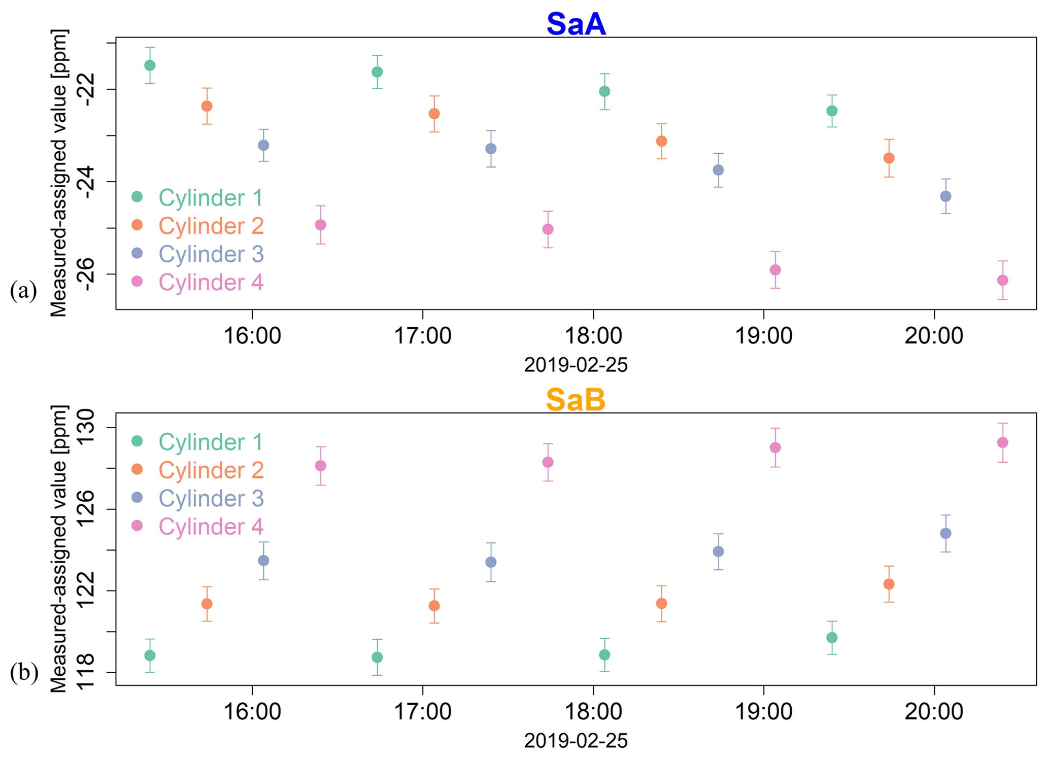
Figure 4Stability of successive CO2 calibrations for SaA (a) and SaB (b); the error bars represent the standard deviation of 2 s averages.
3.2 Temperature and pressure dependence
3.2.1 Temperature sensitivity test
During temperature sensitivity tests, the chamber pressure was kept constant at 950 hPa, while the temperature was gradually changed, as seen in Fig. S4. The temperature ranged between 0 and 45 ∘C, following 9 ∘C increment steps, lasting for 20 min. The sensors' cell temperature exhibited an unstable behavior for chamber temperatures below 25 ∘C, while it was stable, at approximately 57 ∘C, for chamber temperatures above 25 ∘C. However, SaA and SaB behaved oppositely when their cells' temperature changed. Therefore, two scenarios were considered for both sensors.
The first scenario is when the analyzer's cell temperature is stable while the ambient air temperature changes (above 25 ∘C). The trend coefficients of CO2 mole fraction over ambient temperatures were −0.564 and −0.527 for SaA and SaB, respectively (shown in Fig. 5a and c). The second scenario is when both the analyzer's cell and ambient temperatures change simultaneously. In this case, the impact of ambient air temperature changes obtained from the first scenario has been corrected prior to considering the cell temperature changes. The trend coefficients of CO2 mole fraction over cell temperatures were −0.979 and 0.378 for SaA and SaB, respectively (shown in Fig. 5b and d). Consequently, SaA performed better when applying the temperature sensitivity test (high R2, lower standard error).

Figure 5Temperature sensitivity tests in the environment chamber: (a) and (c) represent the first scenario; (b) and (d) represent the second scenario.
3.2.2 Pressure sensitivity test
During the pressure tests, the chamber temperature was maintained at 25 ∘C, and pressure ranged from 600 hPa corresponding to 3 km above sea level (a.s.l.) to 1000 hPa in 100 hPa steps, repeated twice. SaA and SaB performed significantly differently in this test, with the SaB sensor showing increased sensitivity to pressure changes (Fig. 6). Generally, the sensors have an internal pressure correction from the manufacturer, and it is apparently not implemented in SaB. However, SaB performed better in the pressure sensitivity test, with tighter linearity (higher R2) when both tests were accounted for.
From the sensitivity tests presented above, we derived the following equations for both sensors:
where Ccor is the mole fraction after correction for changes. Cobs is the observed mole fraction. Tc represents the analyzer's measurement cell temperature, and Tc0 is the original cell temperature at the start of the measurements. Ta represents the ambient temperature, and Ta0 is the ambient temperature at the start of the measurement. P represents the ambient pressure, and P0 is the ambient pressure at the start of the measurements. The equations are also applied for calibrations.
Replications of temperature and pressure sensitivity tests for SaB at a later stage showed high consistency with the initial results presented above. Both sensors have shown different responses in the tests. Therefore, it is essential to perform both temperature and pressure sensitivity tests for individual sensors to obtain their individual correction equations against temperature and pressure changes. Here, we highly recommend characterizing every individual sensor at least once before any use. We also recommend repeating (e.g., annually) these tests regularly as sensor performances tend to change over time.

Figure 6Pressure sensitivity tests in the environment chamber: (a) and (b) represent SaA results of the repeated pressure tests; (c) and (d) represent SaB results of the repeated pressure tests.
3.3 Manned aircraft test results
SaA and SaB measured consistently with the Picarro G2401-m for atmospheric pressure above 800 hPa (equal to 1.5 km a.s.l.) (see Fig. 7a). Their precision was ± 1.4 ppm (1σ) and ± 1.7 ppm (1σ) at 1 Hz and 0.78 ppm (1σ) and ± 1.1 ppm (1σ) with minute-averaged data, respectively (Fig. 7b), larger than the precisions calculated during the laboratory tests. This degradation was expected due to less optimal measurement conditions. Therefore, the test on the piloted aircraft shows the sensors' precision on board under real flight conditions is within 2 ppm (1σ) at 1 Hz and improves to about 1 ppm (1σ) with minute-averaged data.

Figure 7Manned aircraft results: (a) is the time series, and the gray shaded parts present measurements on the ground and measurements of the gas cylinder; (b) is the correlation between CO2 sensors and G2401-m.
3.4 Unmanned aerial vehicle (UAV) tests and validation
SaB was chosen for field deployments due to technical issues with SaA. SaB was integrated into a quad-rotor to evaluate and validate the performance of the sensor on board a UAV platform during flights. The flight path was over the Athalassa National Forest Park (35.1294∘ N, 33.3916∘ E) in Nicosia, Cyprus (Fig. 8). Four flights were performed on 10 June 2021 from 15:00 to 18:00 LT. The procedure was the following: calibration response curves were obtained before and after the flights. A target gas cylinder was measured for 20 min between each flight to characterize the instrument drift. The sensitivity correction Eq. (2) was then applied to the raw data. It was noted that the measured target gas mole fraction drifted linearly throughout the day (Fig. S5a). To account for that, a time-dependent correction, based on running time, was calculated and applied for calibration sequences (Fig. S5a). Practically, this correction was applied to obtain flight-specific calibration response curves according to the sensor running time and confirmed by the target linear drift (Fig. S5).
Reference CO2 measurements were additionally conducted with another Picarro G2401 on the roof of the Novel Technologies Building (NTL) at the Cyprus Institute (CyI) (Fig. 8), at 174 m a.s.l., 1.82 km northwest upwind from the UAV launching location (187 m a.s.l.). Therefore, the flight path was downwind from the Picarro G2401. The residual values of CO2 between the Picarro and UAV CO2 systems varied from 0.2 to 2.1 ppm (median = 1.1 ppm) during the experiment.

Figure 8The map presents the locations of the Picarro G2401 at CyI, the UAV flight path, Athalassa National Forest Park, and the residential area in Nicosia (© Google Earth 2022).
The field campaign to test operation in real conditions of our UAV CO2 system was performed on 14 May 2021 from early morning 06:00 LT to late afternoon 17:30 LT. It took place above the Athalassa National Forest Park located southeast of CyI in Nicosia, where 16 flights were performed. Each flight lasted approximately 15 min with most of the flight performed at a constant altitude of 50 and 100 m above ground level (a.g.l.) alternatively. The altitudes were determined following security rules. Firstly, the UAV had to maintain a safe distance above the treeline of the forest park. Therefore, the lowest safe altitude to fly the drone was 50 m a.g.l. Secondly, the ceiling of the UAV CO2 flights was set to 100 m a.g.l., following the European regulations (2019/947 and 2019/945; EASA, 2022) for UAV operations in sparsely populated areas (open category A2), with flights permitted up to 120 m a.g.l. The two selected altitudes were used alternatively in order to obtain representative measurements for either horizontal “mapping” or vertical gradients. The vertical gradients were completed at lower altitudes by rooftop measurements in a nearby building. CO2 mole fractions, as well as meteorological conditions, were measured during the flights on the roof of NTL at CyI. CO2 measurements were done using a Picarro G2401 (174 m a.s.l., 16 m a.g.l., 35.141∘ N, 33.381∘ E); wind speed and wind direction were measured using a sonic anemometer Clima Sensor US model 4.920x.x0.00x with a resolution of a wind speed of 0.1 m s−1 and a wind direction of 1∘.
Each pair of 50 and 100 m altitude flights lasted approximately 1 h (including flight time and the time needed to change the dryer and battery on the ground). The 15 cm cartridge filled with magnesium perchlorate (Mg(ClO4)2) was changed every two flights. The first six flights (three pairs) were performed continuously from 06:00 to 09:00 LT, as well as the last six flights from 15:00 to 17:30 LT. In between, four flights (two pairs) took place between 10:00 and 11:00 LT and between 13:00 and 14:00 LT.
According to the meteorological station data, the wind direction in the morning (before 08:00 LT) was from the northwest, with an average wind speed of 1.2 m s−1. Then the wind direction shifted to northeast and southeast during the day before 13:00 LT, with an average wind speed of 0.9 m s−1. Afterwards, the wind shifted back to northwest but with stronger wind speeds (average of 5.3 m s−1).
Figure 9a displays the measured CO2 (ppm) time series from all UAV flights and the Picarro. The CO2 mole fraction measured during the flights in the early morning and evening, when northwesterly winds occurred, was consistent with that measured by the G2401. A CO2 enhancement linked to the morning traffic peak (from 07:00 to 08:00 LT) was detected at all altitudes. Interestingly, the two measurements eventually differed at 10:00 LT, creating a vertical gradient: the CO2 mole fraction measured on board the UAV remained constant, whereas a decrease of about 5 ppm was measured by the G2401 on the ground.
During the day, with the surface wind direction shifting starting 08:00 LT from northwest to northeast and then southeast, the Picarro G2401 progressively sampled air from the Athalassa National Forest Park. The park, with a total area of 8.4 km2, is an oasis of greenery with many trees, shrubs, and grasses located on the southeastern edge of Nicosia. Considering that the inlet of the G2401 is at the same altitude above sea level as the UAV launching location, the lower observed CO2 mole fraction by the G2401 can most likely be attributed to the Athalassa National Forest Park acting as a surface sink taking up CO2. The reduction of traffic after the peak hour can also play a role in the first part of the day, when the air was blowing from the north. At 50 or 100 m height, the constancy of CO2 mole fractions during the day may suggest a different origin for the air sampled depending on the wind direction at these altitudes (wind was not measured on board the UAV). Potential origins may include “regional” air moving above the surface layer or a plume of emissions from the city lofted at a few tens of meters with a stratified air mass above the park.
During the afternoon, the progressive convergence of surface and UAV observations, with a decrease in UAV CO2 values, suggests either a diffusion of the surface signals at altitude or an enhanced atmospheric mixing. This explanation could be supported using an anemometer integrated on board the UAV to provide additional wind data at various heights. UAV-integrated wind measurements would have to be considered for future applications.
A CO2 mapping during the peak traffic hour is shown in Fig. 9c combined with the flight path at 100 m (the red dot represents the launching site). Figure 9b shows the corresponding CO2 time series combined with wind direction (arrow head) and wind speed (arrow length) information. The high mole fraction (20 ppm above background levels) probably originated from local traffic emissions from the main road southwest of the Athalassa National Forest Park (Fig. 8). This finding highlights the capability of the developed UAV CO2 sensor system to detect fast mole fraction changes and the potential to provide useful insights into CO2 emissions close to the ground in urban areas.
From the vertical profiles (Fig. 10), the difference between the 06:00 and 07:00 LT profiles highlights the peak traffic hour. Additionally, we observed an increasing difference (about 3 ppm) between ground level and 50 m a.g.l., followed by a difference (about 0.5 ppm) between 50 m and 100 m a.g.l. from 08:00 to 13:00 LT when the air mass came from the Athalassa National Forest Park with an average wind speed of 0.9 m s−1. This suggests that the CO2 mole fraction measured by the G2401 and UAV CO2 system represents local CO2 characteristics and that the Athalassa National Forest Park acted as a CO2 sink. Later on, between 15:00 and 17:00 LT when the average wind speed increased (5.3 m s−1), the CO2 mole fraction at 50 and 100 m a.g.l. converged towards surface values. This suggests that the observed wind speed enhancement enabled a better mixing of surface signals at altitude. However, the transport of well-mixed regional background air masses at the measurement area could also be an alternative explanation (background CO2 mole fraction is 418.9 ppm). Although we demonstrated the usefulness of UAV measurements to capture horizontal and vertical CO2 gradients in the planetary boundary layer in an urban or peri-urban environment, a definitive explanation of this particular observation would be beyond the scope of this paper.
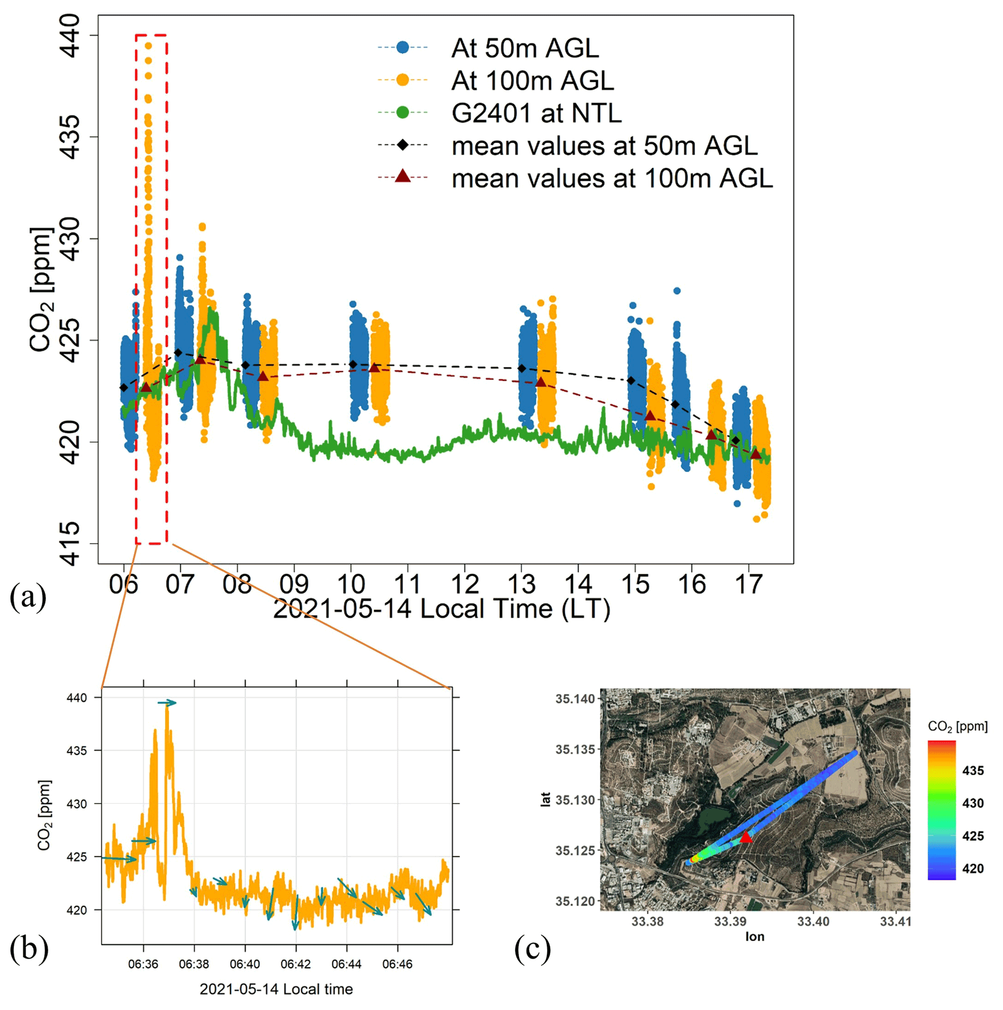
Figure 9(a) Time series of CO2 mole fraction measured by the UAV CO2 sensor (at 50 m in blue and 100 m a.g.l. in orange) and by the Picarro G2401 at CyI (in green). The black diamonds represent the averaged CO2 mole fraction measured by SaB during the flights at 50 m, and the dark red triangles represent the averaged CO2 mole fraction measured by SaB during the flights at 100 m. (b) The corresponding CO2 time series combined with wind direction (arrow head) and wind speed (arrow length) information obtained from the nearby meteorological station, which is a zoom of the second flight marked in the red dashed box in (a). Panel (c) presents the CO2 mapping (the red triangle represents the launching location) during the rush hour (map data: © Google, Maxar Technologies).
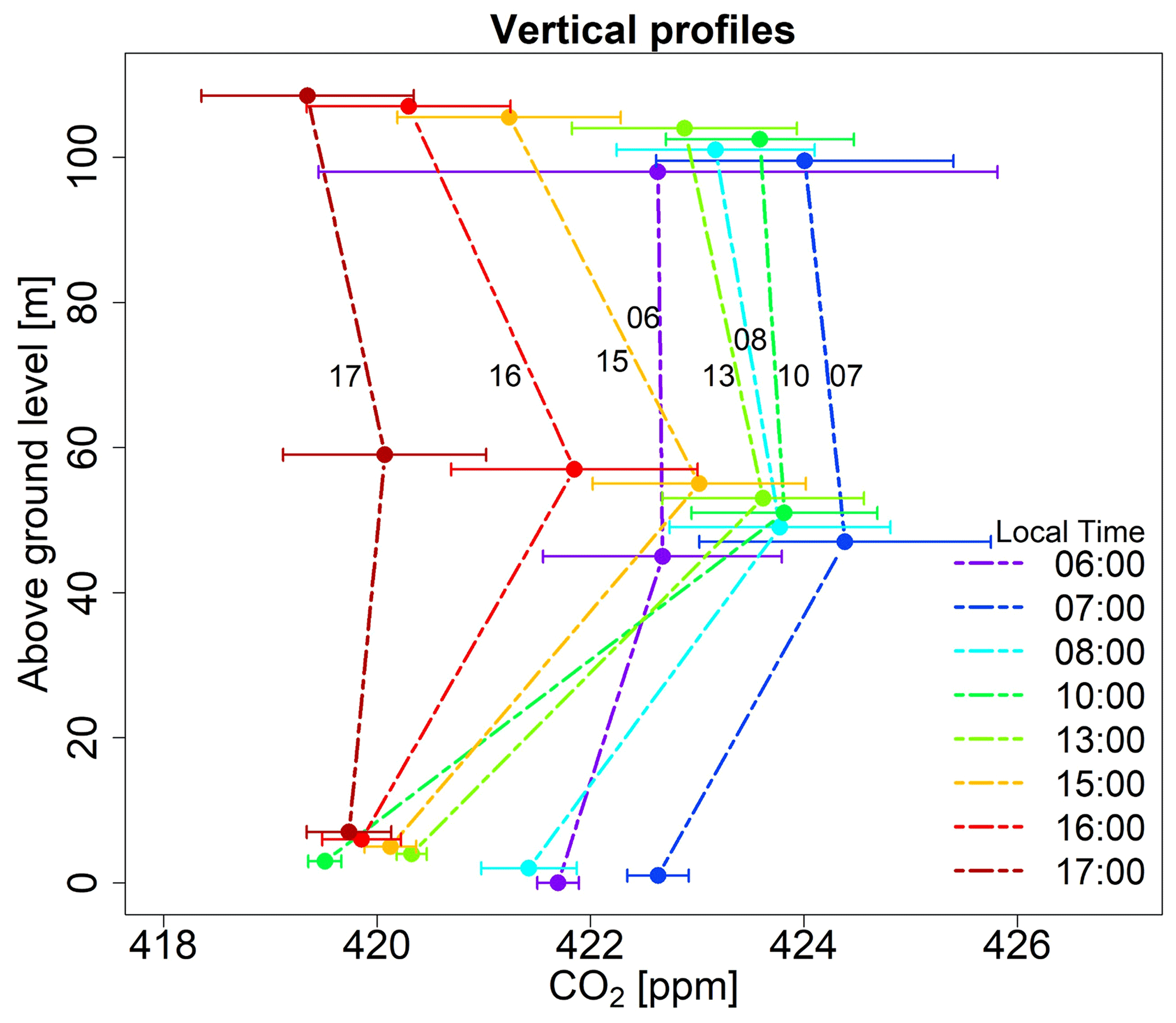
Figure 10Vertical profiles from the eight pairs of flights. The ground level values are from the Picarro G2401 at CyI. CO2 at 50 and 100 m a.g.l. are from the UAV CO2 sensor horizontal flights; the error bars represent the standard deviation of the duration of each flight.
Following the integration of an NDIR CO2 sensor, we developed and validated an autonomous system that can be regarded as a portable package (1058 g), suitable for CO2 measurements on board small UAVs (or other platforms) with good field performance after applying calibration and data corrections (± 1 ppm accuracy for 1 min averages). Prior to deployment, and in order to acquire high-quality observations, the sensor followed a series of quality control procedures. The laboratory tests indicated that the precision was within ± 1 ppm (1σ) at 1 Hz. Two CO2 sensors (SaA and SaB) were tested. It is essential to conduct calibrations before any measurements as shown in this study. NDIR CO2 sensors should not be regarded as plug and play without conducting calibrations and bias correction prior to any measurement campaigns as measurement data would suffer from large, unknown biases without that important step. In general, we advocate that low- and mid-cost sensor units should systematically be characterized for their dependence on pressure and temperature and their factory correction and calibration verified. Strategies for field deployment should also take into account the significant drift that can be observed at the hourly scale. Using a single target gas between flights is sufficient to cope with this drift. Alternative strategies to correct the drift without using gas cylinders on the field remain to be explored, such as comparison against a high-precision instrument at regular intervals during the deployment. Each sensor's performance is impacted by changes in pressure and temperature; therefore, it is necessary to perform pressure and temperature sensitivity tests before any field applications.
Further validation on board a manned aircraft resulted in an estimated precision of ± 2 ppm (1σ) at 1 Hz and ± 1 ppm (1σ) at a 1 min time resolution. During the integration of our system on board a small quadcopter, the calibration strategy was extended to account for running-time-dependent instrumental drifts. Due to its simplicity, the developed system can be replicated easily for wider applications since it has compact, cost-effective, and lightweight advantages. It is anticipated that the integrated portable package can be used in the investigation of emission ratios and fluxes, especially when combined with other sensors on board the UAV platform.
As a proof of concept, the developed system was deployed in a UAV-based flight campaign, where several horizontal flights were performed near the ground and up to 100 m in height. The mole fraction of CO2 up to 440 ppm (20 ppm above the background levels) was detected during the morning traffic rush hour, attributed to emission from a major road located on the southwest of the Athalassa National Forest Park. The CO2 mole fraction measured by the UAV system was consistent with that measured by the Picarro G2401 at CyI when the flight path was downwind of CyI. The system also revealed its ability to capture the temporal variability of the vertical CO2 gradient between the surface and the lower atmosphere. The observed CO2 profiles depict the contribution of traffic emission in the morning from 06:00 to 08:00 LT and also a probable sink due to the Athalassa National Forest Park during the course of the day from 08:00 to 13:00 LT. Furthermore, the measurement system captured the mole fraction drop from 15:00 to 17:00 LT observed at different height levels due to the intensification in the wind speed leading to more horizontal and vertical mixing. In conclusion, the designed system demonstrated its capability to measure fast mole fraction changes and spatial gradients and to provide accurate plume dispersion maps. It proved to be a good complementary measurement tool to the in situ observations performed at the surface.
The data presented in this study are based on many different experiments, given the fact that our experiments and field deployments were aimed at characterizing the two sensors used here. The data are not made publicly available in a repository but can be requested from the corresponding author.
The supplement related to this article is available online at: https://doi.org/10.5194/amt-15-4431-2022-supplement.
YL contributed to the lab experiments' design and setup, field deployments, data collection, data analysis, and writing of the paper. JDP, MV, PB, and JS contributed to project advising, reviewing, and editing the paper. PA, CC, CK, AL, and PV contributed to the miniaturization, integration, and evaluation of the UAV CO2 sensor system, UAS operations, and data collection. OL and CP contributed to the laboratory experiments' setup, design, and advising. PYQ contributed to manned aircraft flight measurements, ground Picarro G2401 and meteorological station measurements and maintenance, data collection, and providing support during UAV CO2 flights. MD contributed to the review and editing of the paper.
The contact author has declared that none of the authors has any competing interests.
Publisher’s note: Copernicus Publications remains neutral with regard to jurisdictional claims in published maps and institutional affiliations.
We would like to thank ICOS teams at LSCE for supporting a series of laboratory tests and aircraft field deployment flights. We are grateful for all the efforts of the technicians, pilots, and software developers from USRL/CARE-C at CyI for their support in the integration and field validation of the UAV CO2 sensor system.
This research has been supported by the project Eastern Mediterranean Middle East-Climate & Atmosphere Research Center (EMME-CARE), which has received funding from the European Union's Horizon 2020 research and innovation program (grant no. EMME-CARE (856612)) and the Cyprus Government, and the project Air Quality Services for clean air in Cyprus (AQ-SERVE) (grant no. INTEGRATED/0916/0016) is co-financed by the European Regional Development Fund and the Republic of Cyprus through the Research and Innovation Foundation.
This paper was edited by Justus Notholt and reviewed by Grant Allen and one anonymous referee.
Agustí-Panareda, A., Massart, S., Chevallier, F., Boussetta, S., Balsamo, G., Beljaars, A., Ciais, P., Deutscher, N. M., Engelen, R., Jones, L., Kivi, R., Paris, J.-D., Peuch, V.-H., Sherlock, V., Vermeulen, A. T., Wennberg, P. O., and Wunch, D.: Forecasting global atmospheric CO2, Atmos. Chem. Phys., 14, 11959–11983, https://doi.org/10.5194/acp-14-11959-2014, 2014.
Allen, G., Hollingsworth, P., Kabbabe, K., Pitt, J. R., Mead, M. I., Illingworth, S., Roberts, G., Bourn, M., Shallcross, D. E., and Percival, C. J.: The development and trial of an unmanned aerial system for the measurement of methane flux from landfill and greenhouse gas emission hotspots, Waste Manage., 87, 883–892, https://doi.org/10.1016/j.wasman.2017.12.024, 2019.
Arzoumanian, E., Vogel, F. R., Bastos, A., Gaynullin, B., Laurent, O., Ramonet, M., and Ciais, P.: Characterization of a commercial lower-cost medium-precision non-dispersive infrared sensor for atmospheric CO2 monitoring in urban areas, Atmos. Meas. Tech., 12, 2665–2677, https://doi.org/10.5194/amt-12-2665-2019, 2019.
Bara, E., Dwayne, T., and Homayoun, N.: Low-Altitude Aerial Methane Concentration Mapping, Remote Sens., 9, 823, https://doi.org/10.3390/rs9080823, 2017.
Barchyn, T., Hugenholtz, C. H., Myshak, S., and Bauer, J.: A UAV-based system for detecting natural gas leaks, J. Unmanned Veh. Sys., 6, 18–30, https://doi.org/10.1139/juvs-2017-0018, 2018.
Barker, P. A., Allen, G., Gallagher, M., Pitt, J. R., Fisher, R. E., Bannan, T., Nisbet, E. G., Bauguitte, S. J.-B., Pasternak, D., Cliff, S., Schimpf, M. B., Mehra, A., Bower, K. N., Lee, J. D., Coe, H., and Percival, C. J.: Airborne measurements of fire emission factors for African biomass burning sampled during the MOYA campaign, Atmos. Chem. Phys., 20, 15443–15459, https://doi.org/10.5194/acp-20-15443-2020, 2020.
Barritault, P., Brun, M., Lartigue, O., Willemin, J., Ouvrier-Buffet, J.-L., Pocas, S., and Nicoletti, S.: Low power CO2 NDIR sensing using a micro-bolometer detector and a micro-hotplate IR-source, Sens. Actuators B: Chem., 182, 565–570, https://doi.org/10.1016/j.snb.2013.03.048, 2013.
Berman, E. S. F., Fladeland, M., Liem, J., Kolyer, R., and Gupta, M.: Greenhouse gas analyzer for measurements of carbon dioxide, methane, and water vapor aboard an unmanned aerial vehicle, Sens. Actuators B Chem., 169, 128–135, https://doi.org/10.1016/j.snb.2012.04.036, 2012.
Bovensmann, H., Burrows, J. P., Buchwitz, M., Frerick, J., Noël, S., Rozanov, V. V., Chance, K. V., and Goede, A. P. H.: SCIAMACHY: Mission Objectives and Measurement Modes, J. Atmos. Sci., 56, 127–150, https://doi.org/10.1175/1520-0469(1999)056<0127:SMOAMM>2.0.CO;2, 1999.
Chiba, T., Haga, Y., Inoue, M., Kiguchi, O., Nagayoshi, T., Madokoro, H., and Morino, I.: Measuring Regional Atmospheric CO2 Concentrations in the Lower Troposphere with a Non-Dispersive Infrared Analyzer Mounted on a UAV, Ogata Village, Akita, Japan, Atmosphere, 10, 487, https://doi.org/10.3390/atmos10090487, 2019.
Crosson, E. R.: A cavity ring-down analyzer for measuring atmospheric levels of methane, carbon dioxide, and water vapor, Appl. Phys. B, 92, 403–408, https://doi.org/10.1007/s00340-008-3135-y, 2008.
Defratyka, S. M., Paris, J.-D., Yver-Kwok, C., Loeb, D., France, J., Helmore, J., Yarrow, N., Gros, V., and Bousquet, P.: Ethane measurement by Picarro CRDS G2201-i in laboratory and field conditions: potential and limitations, Atmos. Meas. Tech., 14, 5049–5069, https://doi.org/10.5194/amt-14-5049-2021, 2021.
EASA (European Union Aviation Safety Agency): Easy Access Rules for Unmanned Aircraft Systems (Regulation (EU) 2019/947 and Regulation (EU) 2019/945), https://www.easa.europa.eu/document-library/easy-access-rules/easy-access-rules-unmanned-aircraft-systems-regulation-eu, last access: 28 March 2022.
Frey, M., Sha, M. K., Hase, F., Kiel, M., Blumenstock, T., Harig, R., Surawicz, G., Deutscher, N. M., Shiomi, K., Franklin, J. E., Bösch, H., Chen, J., Grutter, M., Ohyama, H., Sun, Y., Butz, A., Mengistu Tsidu, G., Ene, D., Wunch, D., Cao, Z., Garcia, O., Ramonet, M., Vogel, F., and Orphal, J.: Building the COllaborative Carbon Column Observing Network (COCCON): long-term stability and ensemble performance of the EM27/SUN Fourier transform spectrometer, Atmos. Meas. Tech., 12, 1513–1530, https://doi.org/10.5194/amt-12-1513-2019, 2019.
Friedlingstein, P., Jones, M. W., O'Sullivan, M., Andrew, R. M., Bakker, D. C. E., Hauck, J., Le Quéré, C., Peters, G. P., Peters, W., Pongratz, J., Sitch, S., Canadell, J. G., Ciais, P., Jackson, R. B., Alin, S. R., Anthoni, P., Bates, N. R., Becker, M., Bellouin, N., Bopp, L., Chau, T. T. T., Chevallier, F., Chini, L. P., Cronin, M., Currie, K. I., Decharme, B., Djeutchouang, L. M., Dou, X., Evans, W., Feely, R. A., Feng, L., Gasser, T., Gilfillan, D., Gkritzalis, T., Grassi, G., Gregor, L., Gruber, N., Gürses, Ö., Harris, I., Houghton, R. A., Hurtt, G. C., Iida, Y., Ilyina, T., Luijkx, I. T., Jain, A., Jones, S. D., Kato, E., Kennedy, D., Klein Goldewijk, K., Knauer, J., Korsbakken, J. I., Körtzinger, A., Landschützer, P., Lauvset, S. K., Lefèvre, N., Lienert, S., Liu, J., Marland, G., McGuire, P. C., Melton, J. R., Munro, D. R., Nabel, J. E. M. S., Nakaoka, S.-I., Niwa, Y., Ono, T., Pierrot, D., Poulter, B., Rehder, G., Resplandy, L., Robertson, E., Rödenbeck, C., Rosan, T. M., Schwinger, J., Schwingshackl, C., Séférian, R., Sutton, A. J., Sweeney, C., Tanhua, T., Tans, P. P., Tian, H., Tilbrook, B., Tubiello, F., van der Werf, G. R., Vuichard, N., Wada, C., Wanninkhof, R., Watson, A. J., Willis, D., Wiltshire, A. J., Yuan, W., Yue, C., Yue, X., Zaehle, S., and Zeng, J.: Global Carbon Budget 2021, Earth Syst. Sci. Data, 14, 1917–2005, https://doi.org/10.5194/essd-14-1917-2022, 2022.
Hazan, L., Tarniewicz, J., Ramonet, M., Laurent, O., and Abbaris, A.: Automatic processing of atmospheric CO2 and CH4 mole fractions at the ICOS Atmosphere Thematic Centre, Atmos. Meas. Tech., 9, 4719–4736, https://doi.org/10.5194/amt-9-4719-2016, 2016.
Hummelgård, C., Bryntse, I., Bryzgalov, M., Henning, J.-A., Martin, H., Norén, M., and Rödjegård, H.: Low-cost NDIR based sensor platform for sub-ppm gas detection, Urban Clim., 14, 342–350, https://doi.org/10.1016/j.uclim.2014.09.001, 2015.
Jacob, D. J., Turner, A. J., Maasakkers, J. D., Sheng, J., Sun, K., Liu, X., Chance, K., Aben, I., McKeever, J., and Frankenberg, C.: Satellite observations of atmospheric methane and their value for quantifying methane emissions, Atmos. Chem. Phys., 16, 14371–14396, https://doi.org/10.5194/acp-16-14371-2016, 2016.
Daube Jr, B. C. D., Boering, K. A., Andrews, A. E., and Wofsy, S. C.: A High-Precision Fast-Response Airborne CO2 Analyzer for In Situ Sampling from the Surface to the Middle Stratosphere, J. Atmos. Ocean. Technol., 19, 1532–1543, https://doi.org/10.1175/1520-0426(2002)019<1532:AHPFRA>2.0.CO;2, 2002.
Kezoudi, M., Keleshis, C., Antoniou, P., Biskos, G., Bronz, M., Constantinides, C., Desservettaz, M., Gao, R.-S., Girdwood, J., Harnetiaux, J., Kandler, K., Leonidou, A., Liu, Y., Lelieveld, J., Marenco, F., Mihalopoulos, N., Močnik, G., Neitola, K., Paris, J.-D., Pikridas, M., Sarda-Esteve, R., Stopford, C., Unga, F., Vrekoussis, M., and Sciare, J.: The Unmanned Systems Research Laboratory (USRL): A New Facility for UAV-Based Atmospheric Observations, Atmosphere, 12, 1042, https://doi.org/10.3390/atmos12081042, 2021.
Khangaonkat, T., Nugraha, A., Xu, W., and Balaguru, K.: Salish Sea response to global climate change, sea level rise, and future nutrient loads, J. Geophys. Res.-Oceans, 124, 3876–3904, https://doi.org/10.1029/2018JC014670, 2019.
Kunz, M., Lavric, J. V., Gerbig, C., Tans, P., Neff, D., Hummelgård, C., Martin, H., Rödjegård, H., Wrenger, B., and Heimann, M.: COCAP: a carbon dioxide analyser for small unmanned aircraft systems, Atmos. Meas. Tech., 11, 1833–1849, https://doi.org/10.5194/amt-11-1833-2018, 2018.
Liu, Y., Zhou, L., Tans, P. P., Zang, K., and Cheng, S.: Ratios of greenhouse gas emissions observed over the Yellow Sea and the East China Sea, Sci. Total Environ., 633, 1022–1031, https://doi.org/10.1016/j.scitotenv.2018.03.250, 2018.
Malaver, A., Motta, N., Corke, P., and Gonzalez, F.: Development and Integration of a Solar Powered Unmanned Aerial Vehicle and a Wireless Sensor Network to Monitor Greenhouse Gases, Sensors, 15, 4072–4096, https://doi.org/10.3390/s150204072, 2015.
Masson-Delmotte, V., Zhai, P., Pörtner, H.-O., Roberts, D., Skea, J., Shukla, P. R., Pirani, A., Moufouma-Okia, W., Péan, C., Pidcock, R., Connors, S., Matthews, J. B. R., Chen, Y., Zhou, X., Gomis, M. I., Lonnoy, E., Maycock, T., Tignor, M., and Waterfield, T. (Eds.): IPCC, 2018: Global Warming of 1.5 ∘C. An IPCC Special Report on the impacts of global warming of 1.5 ∘C above pre-industrial levels and related global greenhouse gas emission pathways, in the context of strengthening the global response to the threat of climate change, sustainable development, and efforts to eradicate poverty, Cambridge University Press, 2018.
Masson-Delmotte, V., Zhai, P., Pirani, A., Connors, S. L., Péan, C., Berger, S., Caud, N., Chen, Y., Goldfarb, L., Gomis, M. I., Huang, M., Leitzell, K., Lonnoy, E., Matthews, J. B. R., Maycock, T. K., Waterfield, T.,Yelekçi, O., Yu, R., and Zhou, B. (Eds.): IPCC, 2021: Climate Change 2021: The Physical Science Basis. Contribution of Working Group I to the Sixth Assessment Report of the Intergovernmental Panel on Climate Change, Cambridge University Press, in press, 2022.
O'Shea, S. J., Allen, G., Gallagher, M. W., Bower, K., Illingworth, S. M., Muller, J. B. A., Jones, B. T., Percival, C. J., Bauguitte, S. J.-B., Cain, M., Warwick, N., Quiquet, A., Skiba, U., Drewer, J., Dinsmore, K., Nisbet, E. G., Lowry, D., Fisher, R. E., France, J. L., Aurela, M., Lohila, A., Hayman, G., George, C., Clark, D. B., Manning, A. J., Friend, A. D., and Pyle, J.: Methane and carbon dioxide fluxes and their regional scalability for the European Arctic wetlands during the MAMM project in summer 2012, Atmos. Chem. Phys., 14, 13159–13174, https://doi.org/10.5194/acp-14-13159-2014, 2014.
OVSQ Essais thermiques: https://www.ovsq.uvsq.fr/essais-thermiques, last access: 9 February 2022.
Pales, J. C. and Keeling, C. D.: The concentration of atmospheric carbon dioxide in Hawaii, J. Geophys. Res., 70, 6053–6076, https://doi.org/10.1029/JZ070i024p06053, 1965.
Paris, J.-D., Ciais, P., Nédélec, P., Ramonet, M., Belan, B. D., Arshinov, M. Yu., Golitsyn, G. S., Granberg, I., Stohl, A., Cayez, G., Athier, G., Boumard, F., and Cousin, J.-M.: The YAK-AEROSIB transcontinental aircraft campaigns: new insights on the transport of CO2, CO and O3 across Siberia, Tellus B Chem. Phys. Meteorol., 60, 551–568, https://doi.org/10.1111/j.1600-0889.2008.00369.x, 2008.
Paris, J.-D., Riandet, A., Bourtsoukidis, E., Delmotte, M., Berchet, A., Williams, J., Ernle, L., Tadic, I., Harder, H., and Lelieveld, J.: Shipborne measurements of methane and carbon dioxide in the Middle East and Mediterranean areas and the contribution from oil and gas emissions, Atmos. Chem. Phys., 21, 12443–12462, https://doi.org/10.5194/acp-21-12443-2021, 2021.
Pinty, B., Janssens-Maenhout, G., M., D., Zunker, H., Brunhes, T., Ciais, P., Denier van der Gon, D. Dee, H., Dolman, H., M., D., Engelen, R., Heimann, M., Holmlund, K., Husband, R., Kentarchos, A., Meijer, Y., Palmer, P., and Scholze, M.: An Operational Anthropogenic CO2 Emissions Monitoring and Verification Support capacity: Baseline Requirements, Model Components and Functional Architecture, European Commission Joint Research Centre, EUR 28736 EN, https://doi.org/10.2760/08644, 2017.
Pitt, J. R., Allen, G., Bauguitte, S. J.-B., Gallagher, M. W., Lee, J. D., Drysdale, W., Nelson, B., Manning, A. J., and Palmer, P. I.: Assessing London CO2, CH4 and CO emissions using aircraft measurements and dispersion modelling, Atmos. Chem. Phys., 19, 8931–8945, https://doi.org/10.5194/acp-19-8931-2019, 2019.
Shah, A., Pitt, J. R., Ricketts, H., Leen, J. B., Williams, P. I., Kabbabe, K., Gallagher, M. W., and Allen, G.: Testing the near-field Gaussian plume inversion flux quantification technique using unmanned aerial vehicle sampling, Atmos. Meas. Tech., 13, 1467–1484, https://doi.org/10.5194/amt-13-1467-2020, 2020.
Suto, H., Kataoka, F., Kikuchi, N., Knuteson, R. O., Butz, A., Haun, M., Buijs, H., Shiomi, K., Imai, H., and Kuze, A.: Thermal and near-infrared sensor for carbon observation Fourier transform spectrometer-2 (TANSO-FTS-2) on the Greenhouse gases Observing SATellite-2 (GOSAT-2) during its first year in orbit, Atmos. Meas. Tech., 14, 2013–2039, https://doi.org/10.5194/amt-14-2013-2021, 2021.
Reuter, M., Bovensmann, H., Buchwitz, M., Borchardt, J., Krautwurst, S., Gerilowski, K., Lindauer, M., Kubistin, D., and Burrows, J. P.: Development of a small unmanned aircraft system to derive CO2 emissions of anthropogenic point sources, Atmos. Meas. Tech., 14, 153–172, https://doi.org/10.5194/amt-14-153-2021, 2021.
Sweeney, C., Karion, A., Wolter, S., Newberger, T., Guenther, D., Higgs, J. A., Andrews, A. E., Lang, P. M., Neff, D., Dlugokencky, E., Miller, J. B., Montzka, S. A., Miller, B. R., Masarie, K. A., Biraud, S. C., Novelli, P. C., Crotwell, M., Crotwell, A. M., Thoning, K., and Tans, P. P.: Seasonal climatology of CO2 across North America from aircraft measurements in the NOAA/ESRL Global Greenhouse Gas Reference Network, 120, 5155–5190, https://doi.org/10.1002/2014JD022591, 2015.
Turner, A. J., Jacob, D. J., Wecht, K. J., Maasakkers, J. D., Lundgren, E., Andrews, A. E., Biraud, S. C., Boesch, H., Bowman, K. W., Deutscher, N. M., Dubey, M. K., Griffith, D. W. T., Hase, F., Kuze, A., Notholt, J., Ohyama, H., Parker, R., Payne, V. H., Sussmann, R., Sweeney, C., Velazco, V. A., Warneke, T., Wennberg, P. O., and Wunch, D.: Estimating global and North American methane emissions with high spatial resolution using GOSAT satellite data, Atmos. Chem. Phys., 15, 7049–7069, https://doi.org/10.5194/acp-15-7049-2015, 2015.
Unmanned systems research laboratory, the Cyprus Institute: https://usrl.cyi.ac.cy/, last access: 28 March 2022.
Watai, T., Machida, T., Ishizaki, N., and Inoue, G.: A Lightweight Observation System for Atmospheric Carbon Dioxide Concentration Using a Small Unmanned Aerial Vehicle, J. Atmos. Ocean. Technol., 23, 700–710, https://doi.org/10.1175/JTECH1866.1, 2006.
WMO GAW Central Calibration Laboratories: https://gml.noaa.gov/ccl/, last access: 9 February 2022.
WMO Greenhouse Gas Bulletin (GHG Bulletin)-No.17: The State of Greenhouse Gases in the Atmosphere Based on Global Observations through 2020, WMO, https://library.wmo.int/doc_num.php?explnum_id=10904 (last access: 28 July 2022), 2021.
Wunch, D., Wennberg, P. O., Osterman, G., Fisher, B., Naylor, B., Roehl, C. M., O'Dell, C., Mandrake, L., Viatte, C., Kiel, M., Griffith, D. W. T., Deutscher, N. M., Velazco, V. A., Notholt, J., Warneke, T., Petri, C., De Maziere, M., Sha, M. K., Sussmann, R., Rettinger, M., Pollard, D., Robinson, J., Morino, I., Uchino, O., Hase, F., Blumenstock, T., Feist, D. G., Arnold, S. G., Strong, K., Mendonca, J., Kivi, R., Heikkinen, P., Iraci, L., Podolske, J., Hillyard, P. W., Kawakami, S., Dubey, M. K., Parker, H. A., Sepulveda, E., García, O. E., Te, Y., Jeseck, P., Gunson, M. R., Crisp, D., and Eldering, A.: Comparisons of the Orbiting Carbon Observatory-2 (OCO-2) XCO2 measurements with TCCON, Atmos. Meas. Tech., 10, 2209–2238, https://doi.org/10.5194/amt-10-2209-2017, 2017.
Wunch, D., Toon, G. C., Blavier, J.-F. L., Washenfelder, R. A., Notholt, J., Connor, B. J., Griffith, D.W. T., Sherlock, V., and Wennberg, P. O.: The Total Carbon Column Observing Network, Philosophical Transactions of the Royal Society of London A: Mathematical, Phys. Eng. Sci., 369, 2087–2112, https://doi.org/10.1098/rsta.2010.0240, 2011.
Xueref-Remy, I., Messager, C., Filippi, D., Pastel, M., Nedelec, P., Ramonet, M., Paris, J. D., and Ciais, P.: Variability and budget of CO2 in Europe: analysis of the CAATER airborne campaigns – Part 1: Observed variability, Atmos. Chem. Phys., 11, 5655–5672, https://doi.org/10.5194/acp-11-5655-2011, 2011.
Yver Kwok, C., Laurent, O., Guemri, A., Philippon, C., Wastine, B., Rella, C. W., Vuillemin, C., Truong, F., Delmotte, M., Kazan, V., Darding, M., Lebègue, B., Kaiser, C., Xueref-Rémy, I., and Ramonet, M.: Comprehensive laboratory and field testing of cavity ring-down spectroscopy analyzers measuring H2O, CO2, CH4 and CO, Atmos. Meas. Tech., 8, 3867–3892, https://doi.org/10.5194/amt-8-3867-2015, 2015.