Polarization performance simulation for the GeoXO atmospheric composition instrument: NO₂ retrieval impacts

NOAA's Geostationary Extended Observations (GeoXO) constellation will continue and expand on the capabilities of the current generation of geostationary satellite systems to support US weather, ocean, atmosphere, and climate operations. It is planned to consist of a dedicated atmospheric composition instrument (ACX) to support air quality forecasting and monitoring by providing capabilities similar to missions such as TEMPO (Tropospheric Emission: Monitoring Pollution), currently planned to launch in 2023, as well as OMI (Ozone Monitoring Instrument), TROPOMI (TROPOspheric Monitoring Instrument), and GEMS (Geostationary Environment Monitoring Spectrometer) currently in operation. As the early phases of ACX development are progressing, design trade-offs are being considered to understand the relationship between instrument design choices and trace gas retrieval impacts. Some of these choices will affect the instrument polarization sensitivity (PS), which can have radiometric impacts on environmental satellite observations. We conducted a study to investigate how such radiometric impacts can affect NO₂ retrievals by exploring their sensitivities to time of day, location, and scene type with an ACX instrument model that incorporates PS. The study addresses the basic steps of operational NO₂ retrievals: the spectral fitting step and the conversion of slant column to vertical column via the air mass factor (AMF). The spectral fitting step was performed by generating at-sensor radiance from a clear-sky scene with a known NO₂ amount, the application of an instrument model including both instrument PS and noise, and a physical retrieval. The spectral fitting step was found to mitigate the impacts of instrument PS. The AMF-related step was considered for clear-sky and partially cloudy scenes, for which instrument PS can lead to errors in interpreting the cloud content, propagating to AMF errors and finally to NO₂ retrieval errors. For this step, the NO₂ retrieval impacts were small but non-negligible for high NO₂ amounts; we estimated that a typical high NO₂ amount can cause a maximum retrieval error of 0.25×10¹⁵ molec. cm⁻² for a PS of 5 %. These simulation capabilities were designed to aid in the development of a GeoXO atmospheric composition instrument that will improve our ability to monitor and understand the Earth's atmosphere.

1 Introduction

NOAA's Geostationary Extended Observations (GeoXO) constellation will continue and expand on the capabilities of the current generation of geostationary satellite systems to support US weather, ocean, atmosphere, and climate operations. It is planned to consist of a dedicated atmospheric composition instrument (ACX) to support air quality monitoring and forecasting. The mission will build on knowledge obtained from low-Earth orbit (LEO) and geostationary (GEO) satellite air quality monitoring instruments such as the TROPOspheric Monitoring Instrument (TROPOMI) (Veefkind et al., 2012), OMI (Ozone Monitoring Instrument) (Levelt et al., 2006, 2018), the Geostationary Environment Monitoring Spectrometer (GEMS) (Kim et al., 2020), and Sentinel 4 (Kolm et al., 2017). Retrievals of trace gases like NO₂ derived from satellite platform observations have been used to relate top-down emissions estimates, air quality monitoring and forecasting, pollution events, trends, and health studies (Bovensmann et al., 2011; Levelt et al., 2018; Burrows et al., 1999; Bovensmann et al., 1999; Levelt et al., 2006; Munro et al., 2016; Bak et al., 2017; Veefkind et al., 2012; Cooper et al., 2022; Hollingsworth et al., 2008). The World Health Organization has designated NO₂ as a pollutant, since it has detrimental effects on human health (World Health Organization, 2021; Huangfu and Atkinson, 2020). It also impacts climate by contributing to the formation of aerosols in the upper troposphere that reflect incoming solar radiation and thus cool the planet (Shindell et al., 2009). Over non-polluted regions, stratospheric NO₂ participates in photochemical reactions that can affect the ozone layer (Crutzen, 1979).

In the near future, these phenomena will be monitored from geostationary (GEO) orbit over greater North America as part of the TEMPO (Troposphere Emission: Monitoring Pollution) mission (Zoogman et al., 2017) at an increased temporal frequency than available from its LEO counterparts. Like other atmospheric composition monitoring instruments, TEMPO is and ACX will be a hyperspectral imager with fine spectral sampling and resolution from the ultraviolet to the near-infrared, allowing trace gas absorption features to be discriminated using the well-known differential optical absorption spectroscopy (DOAS) technique. For total vertical NO₂ amount retrievals, the DOAS technique is applied around the 420 to 455 nm range (Bucsela et al., 2006; Lamsal et al., 2021; Marchenko et al., 2015; Boersma et al., 2007; Richter and Burrows, 2002; Valks et al., 2011; Martin, 2002).

ACX is in its early stages of development with its initial performance requirements being formulated with respect to parameters like sampling and resolution to enable this DOAS approach. Other parameters such as pixel size, noise, and polarization sensitivity (PS) are also being defined. These requirements may be updated as the instrument design choices are better understood. This study focuses on the requirements for instrument PS, which, for instance, may provide information on whether a polarization scrambler is needed. Air quality monitoring instruments such as OMI and TROPOMI were designed with polarization scramblers to reduce their PS (Bézy et al., 2017; Voors et al., 2017).

Without PS suppression, the polarization state of incoming radiation will impact the at-sensor radiance for satellite sensors in both GEO (Pearlman et al., 2015) and LEO, though these impacts have been more extensively analyzed for LEO satellites (Meister and Franz, 2011; Wu et al., 2017; Goldin et al., 2019). GEO orbit presents unique challenges due to the highly variable solar angles throughout the day. This results in variation in the degree of linear polarization of the at-sensor radiance throughout the day due to Rayleigh scattering in the Earth's atmosphere; for instance, light scattered in the normal direction to the incident light generates highly polarized radiation but not in the forward or backward direction. If the instrument is sensitive to light with a certain polarization, this variation in degree of linear polarization translates to a variation in measured radiance throughout the day. Thus, limiting the PS of the satellite sensor can limit the radiometric uncertainty. These impacts can be derived by employing radiative transfer simulations to predict the at-sensor polarization state or Stokes parameters (S) and applying the instrument polarization impacts via its Mueller matrix (M).

$$\begin{array}{}\text{(1)}& \begin{array}{rl}& S={\left[S_{\mathrm{0}}{S}_{\mathrm{1}}{S}_{\mathrm{2}}{S}_{\mathrm{3}}\right]}^t\\ & {\mathbf{S}}^{\prime }=\mathbf{M}S\end{array}\end{array}$$

The Stokes formulation expresses the polarization state consisting of its un-polarized (or randomly polarized) component, S₀. Two terms describe its linear polarization state: the excess in horizontal linear polarization relative to the vertical direction, S₁, and excess in linear polarization at 45^∘ relative to 135^∘, S₂. One term describes its circular polarization through its excess of right circular relative to left circular polarization, S₃. The Mueller matrix is a 4×4 matrix used to apply the optical effects of an element to generate an output Stokes vector. We model ACX as a Mueller matrix with a transmission of 1 and nonzero linear polarization extinction elements (m₀₁, m₀₂, m₁₀, and m₂₀). Since the system only detects total energy or radiance, not polarization state, only the first row is relevant. So the output term corresponding to the detected normalized Stokes parameter is

$$\begin{array}{}\text{(2)}& S_{\mathrm{ACX}}^{\prime }=\mathrm{1}+m_{\mathrm{01}}{S}_{\mathrm{1}}+m_{\mathrm{02}}{S}_{\mathrm{2}}.\end{array}$$

This detected radiance can differ from the true at-sensor radiance if ACX has linear PS, defined as $\sqrt{(m_{\mathrm{01}}^{\mathrm{2}}+m_{\mathrm{02}}^{\mathrm{2}})}$, which can propagate to higher-level satellite products. For instance, the retrieval of surface reflectance can suffer from large uncertainties, especially when the signal from the surface is small compared to the atmospheric component. In this work, we discuss our study of NO₂ retrievals and investigate the parts of the process that may be affected. To our knowledge, NO₂ retrieval dependences on instrument PS have not yet been fully documented. We describe an initial study to show the ways that these retrievals can be impacted and make initial estimates of those impacts associated with the current PS requirements: <5 % PS for wavelengths <500 nm.

Our NO₂ retrieval simulation approach discussed here follows a simplified version of the DOAS technique used for operational NO₂ retrievals and consists of two basic steps: one involves the DOAS spectral fitting step for the at-sensor radiance. This fit is normally used to retrieve the NO₂ slant column amount – the total number of molecules along the atmospheric photon path to the satellite sensor. The second step converts this slant column amount to the vertical column amount through the air mass factor (AMF), which depends on the geometrical path as well as the differences in scattering and absorption within the atmosphere between the slant and vertical paths. Our first approach for analyzing polarization effects deals with the DOAS spectral fitting step with clear-sky scenes by simulating at-sensor Stokes parameters and applying an instrument model that includes a range of PS values in several orientations (defined by m₀₁ and m₀₂), as well as the instrument noise and spectral properties consistent with our current knowledge of ACX. The fits of these spectra are used to retrieve NO₂ vertical column amount directly, not slant column, in our case; since these are simulations with the vertical profiles used as inputs, we do not need to use the AMF for converting slant column to vertical column amount. The second approach deals exclusively with the AMF derivation step. For this analysis, the AMF, required for operational retrievals, is affected by instrument PS when considering the potential for partially cloudy scenes. Retrievals in such situations are commonly performed for atmospheric monitoring instruments, since their large instantaneous fields of view make completely clear scenes rare. We will discuss the formalism in detail for both approaches in the Methods section. With these two approaches, referred to as the methods for “clear scenes” and “partially cloudy scenes”, we demonstrate the capability to investigate PS requirements.

2 Methods

As mentioned, the approach for clear scenes exploits the spectral features in the radiance spectra to retrieve the total vertical amount of NO₂, and the approach for cloudy scenes relies on the AMF calculation.

2.1 Clear scenes

The overall method for clear scenes is illustrated in Fig. 1. In this process, simulated radiance spectra are propagated through an instrument model, and the total vertical column NO₂ is retrieved using a look-up table (LUT) approach with the aid of a constrained energy minimization algorithm (CEM) algorithm (Farrand, 1997). Further details are discussed below.

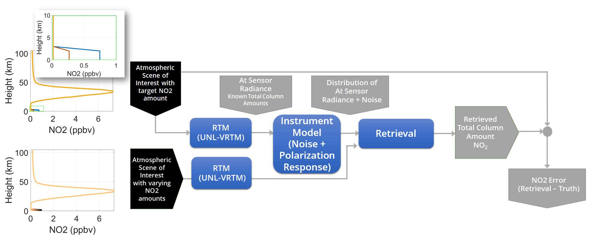
Figure 1 Simulation method for retrieving NO₂ in clear scenes: the scenes of interest consist of selected custom NO₂ profiles to represent low, medium, and high NO₂ cases shown at the upper left (including a zoomed-in view) corresponding to total vertical NO₂ amounts of 4.60, 5.93, and 8.44×10¹⁵ molec. cm⁻², respectively. The lower left profiles contain all profiles used in the retrieval process. The profiles are used in the radiative transfer model (RTM) called the Unified Linearized Vector Radiative Transfer Model (UNL-VRTM) to generate at-sensor radiance.

2.1.1 Radiative transfer modeling

The at-sensor radiances from clear scenes are simulated using a vector radiative transfer code, the Unified Linearized Vector Radiative Transfer Model, UNL-VRTM, which integrates the linearized vector radiative transfer (VLIDORT) into a broader framework (Xu and Wang, 2019). The code can generate Stokes vectors from any scene defined by its view and solar geometry, surface reflectance, wavelength range, and atmospheric composition. Note that rotational Raman scattering is not included in the model. The ACX was assumed to be at 105^∘W longitude, viewing several locations across the continental US (CONUS). The time of day was chosen to generate solar zenith angles of 60 to 70^∘, at which PS is expected to be highest but still within the range in which NO₂ retrievals are typically performed. The US Standard Model default profiles were used for 21 trace gases for all scenes (excluding NO₂). The default NO₂ profiles were modified by injecting a known amount uniformly into the troposphere below 2 km (Fig. 1). Three basic surface spectra generated from spectral libraries were used. The water spectrum used is associated with an open-ocean case (Kokaly et al., 2017). The vegetation is a combination of trees (30 %), grass (30 %), shrubs (30 %), non-photosynthetic material (5 %), and soil (5 %). The urban case is a combination of roof (50 %), concrete (20 %), road (20 %), and vegetation (10 %) (Meerdink et al., 2019; Baldridge et al., 2009) as depicted in Fig. 2. Their associated background aerosol content was included in the boundary layer up to 2 km with a uniform vertical distribution. The rural and urban scenes use a bimodal aerosol distribution as shown in Table 1, where the loading and size distribution values for each mode are given for these scenes. The aerosol parameters including the complex indices of refraction per wavelength were taken from Shettle and Fenn (1979) (with mean values listed in Table 1) and aerosol optical depth (AOD) values from the climatology reported in Yan et al. (2021).

Figure 2 Basic surface reflectance spectra used in radiative transfer simulations: (a) water, (b) vegetation, and (c) urban. (d) Spectra in the NO₂ retrieval spectral range.

Table 1 UNL-VRTM parameters.

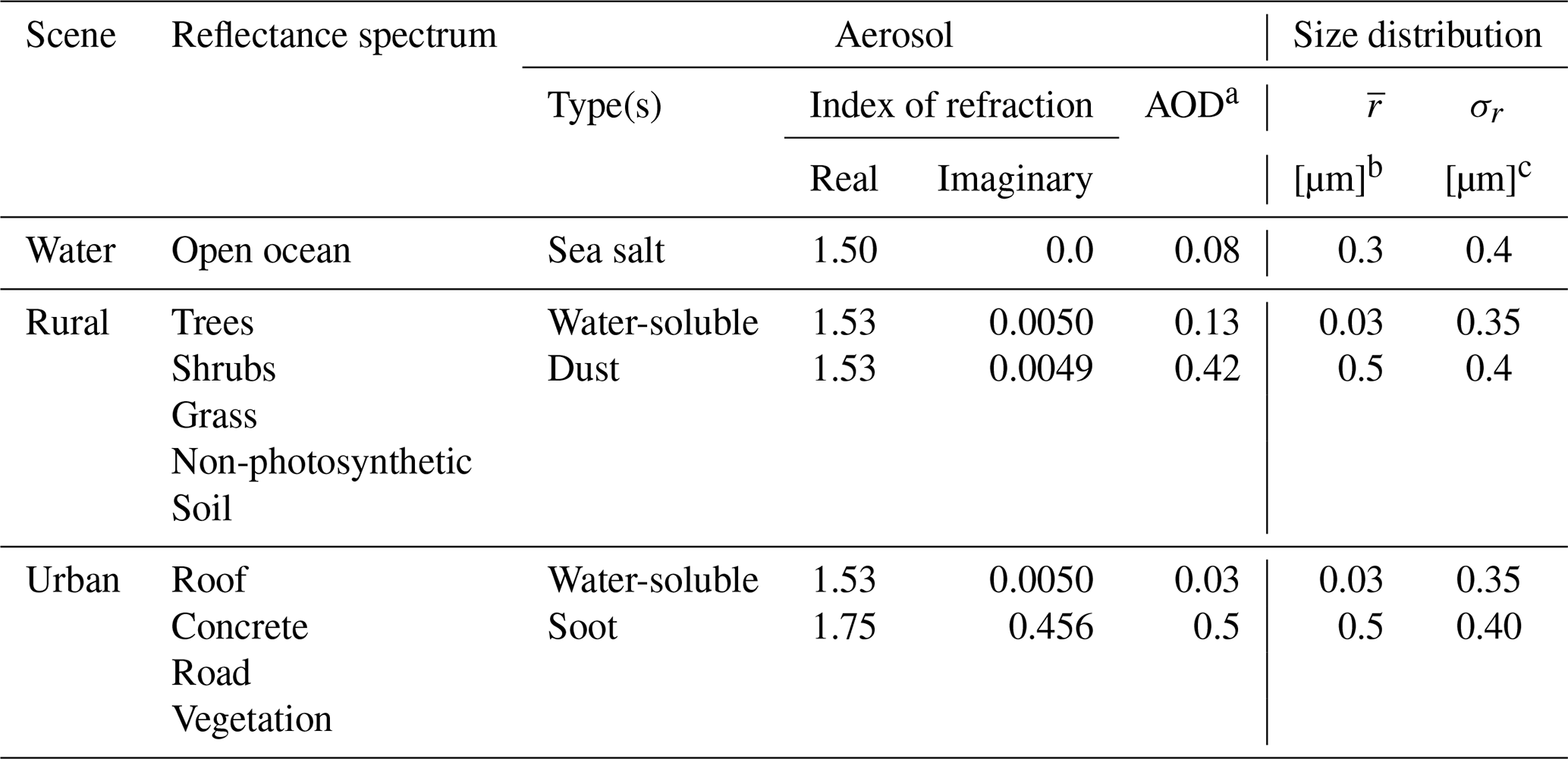
^a Aerosol optical depth. ^b Radius mean. ^c Radius standard deviation.

We ran radiative transfer simulations for several US locations with the three scene types, with varying amounts of tropospheric NO₂. This produced a look-up table (LUT) of scene type, NO₂ vertical amount, and at-sensor radiance spectra. This LUT was used in the retrieval discussed below.

2.1.2 Instrument model and NO₂ retrievals

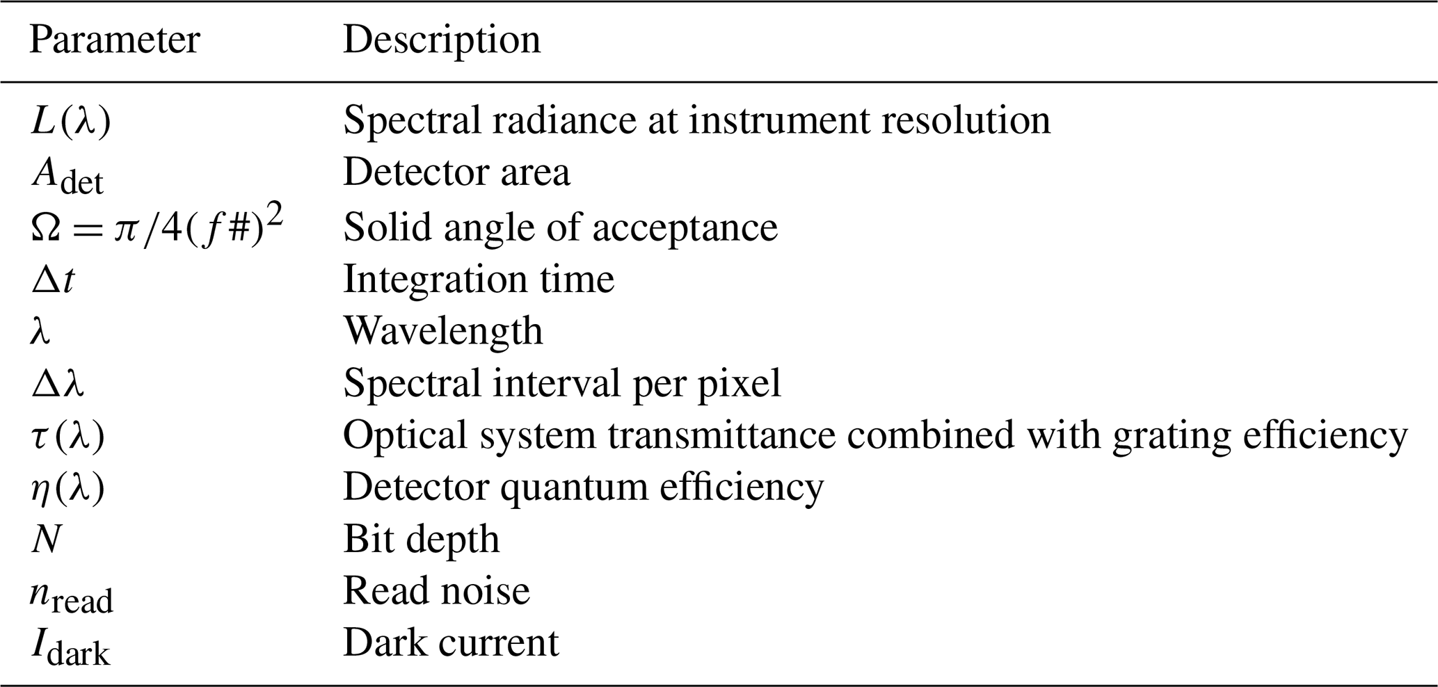
The reference radiance spectra corresponding to the NO₂ reference amounts over water as well as rural and urban scenes were modified by applying the instrument model (for several US locations). The instrument response model was based on the TEMPO design, which consists of a reflective $f/\mathrm{3}$ Schmidt-form telescope and a spectrometer assembly that utilizes a diffraction grating to form an image on charge-coupled device (CCD) detector arrays (Zoogman et al., 2017). The simulated radiance was modified by this instrument response model, which sampled the radiance at 0.2 nm wavelength steps with a resolution of 0.6 nm and applied a PS response. The PS response model was not specific to TEMPO as our goal was to understand the range of impacts associated with the ACX polarization requirements. The noise was also applied as defined by the ACX signal-to-noise ratio (SNR) specification. Our instrument parameters from TEMPO were modified by assuming a sampling strategy or integration time modification that brought the noise in line with that specified by ACX. Table 2​​​​​​​ shows the parameters included in this model.

Table 2 ACX instrument response model parameters.

The noise was applied by generating 1000 spectra with different amounts of noise following a Gaussian distribution that are added to the at-sensor radiance (after being modified by the polarization response). All spectra were normalized by subtracting a second-order polynomial fit to remove the sensitivity to absolute radiance as is done in the DOAS retrieval technique. The NO₂ vertical amount was retrieved using the look-up table and the CEM algorithm:

$$\begin{array}{}\text{(3)}& \text{CEM}={\displaystyle \frac{(t-m{)}^T{C}^{-\mathrm{1}}(x-m)}{(t-m{)}^T{C}^{-\mathrm{1}}(t-m)}},\end{array}$$

where C⁻¹ and m are the inverse covariance matrix and mean over the noise spectra, respectively. The CEM was calculated for all (target) spectra in the LUT, t, with the noise spectra, C⁻¹ and m. The spectrum, x, that generated a CEM value closest to 1 was chosen, and its associated NO₂ vertical amount was retrieved.

2.2 Partially cloudy scenes

The process for “partially cloudy scenes” involves an AMF derivation process that includes the consideration of subpixel-scale clouds. The typical instantaneous field of view for atmospheric composition instruments means that most scenes contain some clouds. Operational trace gas retrievals are routinely done in partially cloudy scenes, so we derive PS impacts for such scenes primarily through their impact on the AMF.

2.2.1 Theoretical background

This approach assumes a simple cloudy scene model with each scene assumed to be a combination of a fully cloud-covered subpixel and a clear-sky subpixel weighted with an effective cloud fraction, f, consistent with previous approaches (Stammes et al., 2008):

$$\begin{array}{}\text{(4)}& L_{\mathrm{obs}}=L_{\mathrm{clr}}(\mathrm{1}-f)+L_{\mathrm{cld}}f,\end{array}$$

where L_obs is the observed radiance, L_clr is the calculated radiance in a clear sky, and L_cld is the cloudy radiance. To produce observed amounts of Rayleigh scattering and absorption, it was found that for this equation to work across most conditions, we model L_cld as a Lambertian surface (opaque) with surface reflectivity 0.80 at the effective cloud pressure, assumed here to be equivalent to a cloud at 2 km. Aerosols are not considered for the cloudy scenes, since they would have a negligible impact; the clouds would lie above the tropospheric NO₂ and aerosol layer. This simple model has been demonstrated to represent the complex radiative transfer in clouds accurately (Stammes et al., 2008; Joiner, 2004; Vasilkov et al., 2008). So, we typically derive f at a wavelength with little absorption and use a surface climatology for L_clr. Then, we simply invert the above equation to give

$$\begin{array}{}\text{(5)}& f={\displaystyle \frac{L_{\mathrm{obs}}-L_{\mathrm{clr}}}{L_{\mathrm{cld}}-L_{\mathrm{clr}}}}.\end{array}$$

For the trace gas retrievals, another quantity defines the fraction of scene radiance from the cloud versus the clear parts of the scene called the cloud radiance fraction, f_r, which has wavelength dependence:

$$\begin{array}{}\text{(6)}& f_{\mathrm{r}}=f{\displaystyle \frac{L_{\mathrm{cld}}}{L_{\mathrm{obs}}}}.\end{array}$$

A cloudy air mass factor (AMF) is computed along with the clear-sky AMF. The total AMF is then computed with the clear and cloudy AMFs weighted by the cloud radiance fraction:

$$\begin{array}{}\text{(7)}& {\text{AMF}}_{\mathrm{total}}={\text{AMF}}_{\mathrm{clr}}\left(\mathrm{1}-f_{\mathrm{r}}\right)+{\text{AMF}}_{\mathrm{cld}}{f}_{\mathrm{r}}.\end{array}$$

To compute the error in the NO₂ vertical column due to an error in f, we started with the calculation of the error in f due to an error from PS,

$$\begin{array}{}\text{(8)}& {\displaystyle \frac{\mathrm{d}f}{\mathrm{d}{\mathit{ϵ}}_{\mathrm{PS}}}}={\displaystyle \frac{\mathrm{d}{L}_{\mathrm{obs}}}{\mathrm{d}{\mathit{ϵ}}_{\mathrm{PS}}}}{\displaystyle \frac{\mathrm{1}}{\left(L_{\mathrm{cld}}-L_{\mathrm{clr}}\right)}},\end{array}$$

and this would then propagate into the error in NO₂ vertical column density (NO_2,VCD) through Eqs. (6) and (7) above, along with

$$\begin{array}{}\text{(9)}& {\mathrm{NO}}_{\mathrm{2},\mathrm{VCD}}={\displaystyle \frac{{\mathrm{NO}}_{\mathrm{2},\mathrm{SCD}}}{{\text{AMF}}_{\mathrm{total}}}}.\end{array}$$

This process is shown graphically in Fig. 3, where a clear and cloudy version of a scene are simulated. The clear version is propagated through the instrument polarization response model, and, using the radiance generated from the cloudy scene, the impacts are propagated through the cloud fraction, cloud radiance fraction, AMF, and finally the NO₂ amount. Following the process by Kuhlmann et al. (2015), the AMFs for each atmospheric layer (also called box AMFs) were computed using a pre-calculated LUT with input parameters of altitude, z, solar zenith angle, view zenith angle, relative azimuth angle, surface reflectance, and surface altitude. The total AMF was calculated by linearly interpolating over all variables for each altitude and summing over all layers to the top of atmosphere (TOA), with each layer dz having a vertical column amount $V_{{\mathrm{NO}}_{\mathrm{2}}}$:

$$\begin{array}{}\text{(10)}& {\text{AMF}}_{\mathrm{clr}/\mathrm{cld}}={\displaystyle \frac{{\int }_{\mathrm{0}}^{\mathrm{TOA}}\mathit{\alpha }\cdot \text{AMF}\left(z\right)\cdot V_{{\mathrm{NO}}_{\mathrm{2}}}\mathrm{d}z}{{\int }_{\mathrm{0}}^{\mathrm{TOA}}{V}_{{\mathrm{NO}}_{\mathrm{2}}}\mathrm{d}z}},\end{array}$$

where the integration assumes an exponential dependence within each layer. A correction term, α, is normally included in the AMF calculation to account for the temperature dependence of the NO₂ cross sections, though it was neglected here by setting it to 1. The NO₂ error derived through the conversion of slant to vertical amount is then computed. This error can be considered the effect of a change in detected radiance due to PS, which, in turn, leads to an error in the interpretation of the amount of cloud in the scene. This leads to an impact on the NO₂ retrieval over the total vertical column. Note that, assuming a constant PS over the wavelength range, this error will also change negligibly as a function of wavelength. We perform this analysis at one wavelength (425.8 nm) in this study. By differentiating Eq. (9), the NO₂ error in the total vertical column amount $(\partial ({\mathrm{NO}}_{\mathrm{2},\mathrm{total}}\left)\right)$ is then calculated in terms of the total vertical NO₂ amount $\left(V_{{\mathrm{NO}}_{\mathrm{2}},\mathrm{total}}\right)$, the AMF, and the AMF error (∂AMF_total) as

$$\begin{array}{}\text{(11)}& \partial \left({\mathrm{NO}}_{\mathrm{2},\mathrm{total}}\right)={\displaystyle \frac{-V_{{\mathrm{NO}}_{\mathrm{2}},\mathrm{total}}}{{\text{AMF}}_{\mathrm{total}}}}\cdot \partial \left({\text{AMF}}_{\mathrm{total}}\right).\end{array}$$

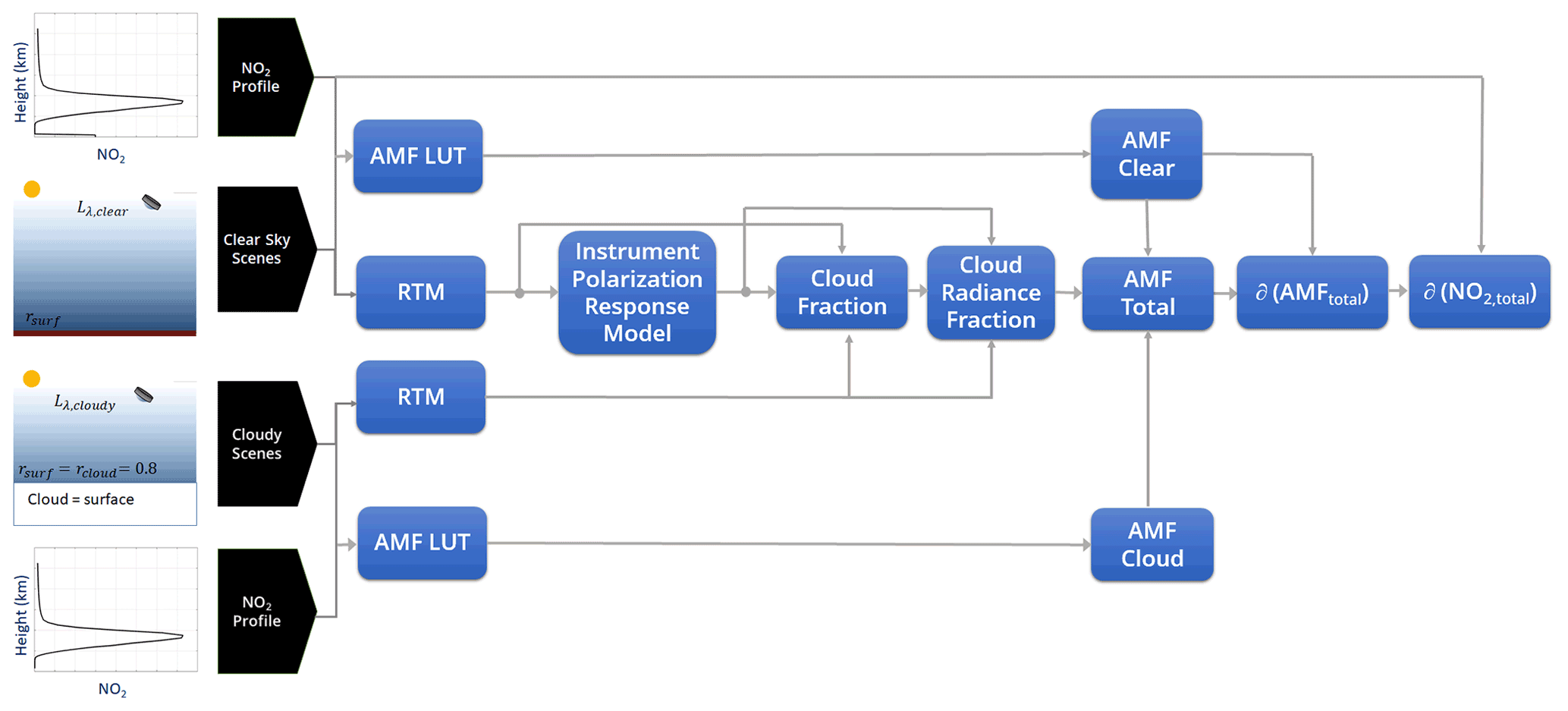
Figure 3 Simulation method for deriving NO₂ errors by interpreting a clear scene as a partially cloudy scene due to instrument PS: through a radiative transfer model (RTM) and air mass factor (AMF) calculations via a look-up table (LUT) of clear and cloudy scenes, as well as applying the instrument polarization response model to a clear scene, the NO₂ error is determined by propagating through the variables shown to errors in AMF (∂(AMF_total)) and total vertical NO₂ amount ($\partial \left({\mathrm{NO}}_{\mathrm{2},\mathrm{total}}\right)$).

2.2.2 Radiative transfer modeling

We conducted the radiative transfer simulations as summarized in Table 3. Simulation A will be shown to define an upper bound for the retrieval error with a PS of 5 % by using an NO₂ profile (similar to those defined in the clear scene simulations) with a large NO₂ amount, the lowest reflectance scene, and high constant solar zenith angle over all of CONUS over a 1^∘ latitude–longitude grid. Simulation B quantifies the retrieval impact of scene type – water, rural, and urban scene – over CONUS for a constant reference NO₂ profile. The scene types are the same as defined in Table 1 and are assigned to all pixels in CONUS for each run. Simulation C explores the retrieval impacts on the solar zenith angle and NO₂ amount for selected US locations. The PS is also varied over a wider range of values. Finally, Simulation D uses NO₂ profiles from GEOS-Chem model data that utilize inputs from the Goddard Earth Observing System Model, Version 5 (GEOS-5) (Molod et al., 2012; Zoogman et al., 2017), on a particular time and day with a fixed scene type over the CONUS grid. Simulations A–C give a contrived version that is useful for bounding the impacts of instrument PS and isolating impacts of different variables. Simulation D represents cases with more realistic nominal parameters. Note that we also used the cloud fraction from the GEOS-Chem model for deriving the simulated radiance prior to applying the polarization response model. This deviates from the illustration in Fig. 1 (top left), where instead of a clear scene, a mixture of cloudy and clear scene according to the GEOS-Chem cloud fraction value is used, thereby accounting for the radiance polarization state of both clear and cloudy scenes in generating the NO₂ retrieval errors. A single day was chosen to demonstrate this approach: 15 July 2007 at two selected times of 16:00 and 20:00 UTC so that the impacts of extreme solar zenith angles (corresponding to high degree of linear polarization) could be seen for both the eastern and western US regions.

Table 3 ACX radiative transfer simulation for cloudy scenes.

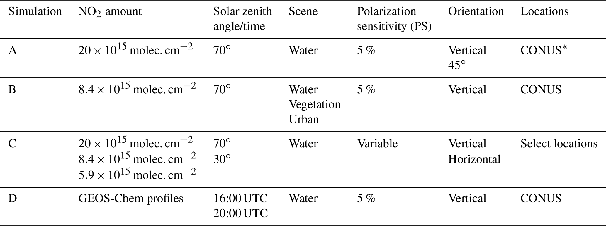
^∗ Continental United States.

3 Results

3.1 Clear scenes

As part of the method for clear scenes, the ACX instrument model was applied to the at-sensor radiance including sampling with a Gaussian slit function at the interval and resolution of 0.2 and 0.6 nm, respectively, as well as its noise as depicted in Fig. 4. The differences between the normalized solar irradiance (multiplied by a factor of 5 for visibility) and radiance spectra show the atmospheric contribution and the effects of this resampling. The 1000 radiance spectra shown cannot be discerned clearly given the high SNR (explicitly shown by the blue line). The noise was applied after modifying with the PS response. The PS model parameters were applied via Eq. (2) using $m_{\mathrm{01}}=\pm \text{PS}$ and m₀₂=0 so that the PS was applied in the vertical or horizontal orientation. These orientations were chosen for most simulations for simplicity, but other orientations will be discussed in the cloudy scene analysis.

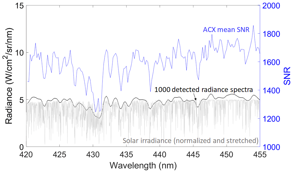
Figure 4 Example of at-sensor radiance spectra simulated with an applied instrument model including resampling effects and an added noise set by ACX instrument parameters. A total of 1000 spectra are plotted (black lines), which appear as lines slightly thicker than the mean SNR (blue line and right axis). The normalized solar irradiance multiplied by a factor of 5 is shown for comparison to the resampled spectra.

The retrieval process effectively matches the spectral shape of the simulated detected spectra – affected by spectral sampling, noise, and PS – to the most similar spectra in the LUT that contains a large range of tropospheric NO₂ amounts for the three surfaces. Figure 5a shows an example of a the adjusted sample spectrum with the spectra in the LUT. Note that all spectra were adjusted using quadratic fits in the spectral fitting process. The CEM algorithm finds the spectrum from the spectra that is most similar. Figure 5b shows a summary of the NO₂ retrieval errors, average biases, and standard deviations as a function of PS for several scene types for a particular location (Norman, Oklahoma). The errors are driven by a combination of the SNR, view and solar geometry, surface reflectance spectrum, and aerosol model and are similar for all scene types. The flat dependence indicates that the PS does not affect the retrieval error in the DOAS spectral fitting retrieval step. The reason is that the PS is a smooth function of wavelength, and the radiometric errors introduced are compensated for through the spectral fitting process. These results were similar for all locations (not shown). We note that other retrieval techniques that do not use a polynomial correction term in the spectral fitting approach may exhibit larger PS impacts.

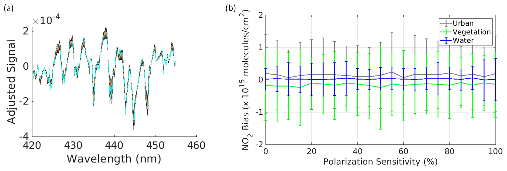
Figure 5 Clear-sky scene retrieval results: (a) an example of an adjusted ACX-simulated spectrum (cyan) with all spectra from the look-up table (LUT) with varying amounts of tropospheric NO₂. (b) The average error (or bias) and standard deviation for 1000 total vertical NO₂ retrievals of the “high” amount (8.44×10¹⁵ molec. cm⁻²) for the three scene types (water, vegetation, and urban) at Norman, Oklahoma, assuming a vertical PS orientation.

3.2 Partially cloudy scenes

In contrast to the previous results, the AMF-related processing step showed more significant polarization impacts, with an error induced when a clear scene is interpreted as a partially cloudy scene due to the instrument response model that includes PS (but not noise). Figure 6 shows the results as they are propagated through each step in the process (Fig. 3) for an example with an extremely high total vertical NO₂ amount of 20×10¹⁵ molec. cm⁻² over all of CONUS (Table 3, Simulation A). The simulation ran using 70^∘ solar zenith angle and water scene for all pixels as well as an instrument PS of 5 %, $m_{\mathrm{01}}=-\mathrm{0.05}$, vertical orientation and m₀₂=0.05, 45^∘ orientation, and an initial cloud fraction of zero. The Stokes parameter, S₁, is relevant for vertical (or horizontal) polarization, and S₂ is relevant for 45^∘ (or 135^∘) polarization. The correlations between the relevant Stokes parameters, retrieved cloud fraction, and NO₂ error are particularly apparent. This example shows that the PS orientation can generate vastly different spatial dependence in NO₂ retrieval errors. The maximum NO₂ error of 1.4×10¹⁵ molec. cm⁻² is above the specified TEMPO NO₂ precision (Zoogman et al., 2017). Note that this is likely an upper bound, since NO₂ amounts like these are mostly found in industrialized areas in other regions of the world.

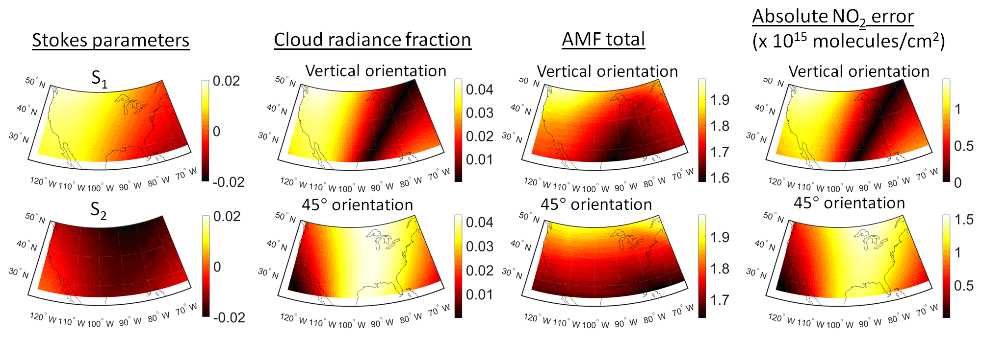
Figure 6 Derived parameters for NO₂ amount of 20×10¹⁵ molec. cm⁻², water scenes, and 5 % PS in a vertical and 45^∘ orientation (see Table 3, Simulation A for more details).

Similar simulations for more realistic NO₂ amounts using constant profiles across CONUS show how these retrieval errors change as a function of surface type (Table 3, Simulation B). Figure 7 shows a lower, more realistic NO₂ amount of 8.4×10¹⁵ molec. cm⁻² corresponding to the “high” NO₂ case shown in Fig. 1. The results are shown for the three different scene types applied uniformly across all of CONUS. The other parameters are the same as the previous higher NO₂ case. The NO₂ error increases as the surface reflectance decreases. All cases show the same spatial pattern over CONUS as in the previous case. The maximum NO₂ error is 0.25×10¹⁵ molec. cm⁻².

Figure 7 NO₂ errors assuming different scene types across CONUS for 5 % PS in a vertical orientation and constant NO₂ profiles with 8.4×10¹⁵ molec. cm⁻² (see Table 3, Simulation B for more details.)

Figure 8 shows the results repeating similar simulations with different NO₂ amounts and times of day for select US locations and their (nonlinear) dependence on PS (Table 3, Simulation C). The figure shows that derived NO₂ errors decrease as the NO₂ amounts decrease using three different total vertical amounts of 5.9, 8.4, and 20×10¹⁵ molec. cm⁻² as a function of PS and two different orientations. The dependence on NO₂ amount is nonlinear; for instance, at 5 % PS for the Seattle evening case, the retrieval errors for increasing amounts are 0.22 %, 2.6 %, and 6.6 %. The time of day dependence is illustrated by the edge of the shading: the darker shading shows the retrieved NO₂ amount with a solar zenith angle of 30^∘, and the edge of the lighter shading shows the amount with an angle of 70^∘. The shading is meant to emphasize the difference between the reference and retrieved amount. The horizontal orientation results are similar to those for the vertical orientation. As evident in the previous results, the largest NO₂ errors occur in the western regions (Seattle, San Diego) for these orientations. The lower solar zenith angle corresponds to a lower degree of linear polarization, accounting for the lower NO₂ errors.

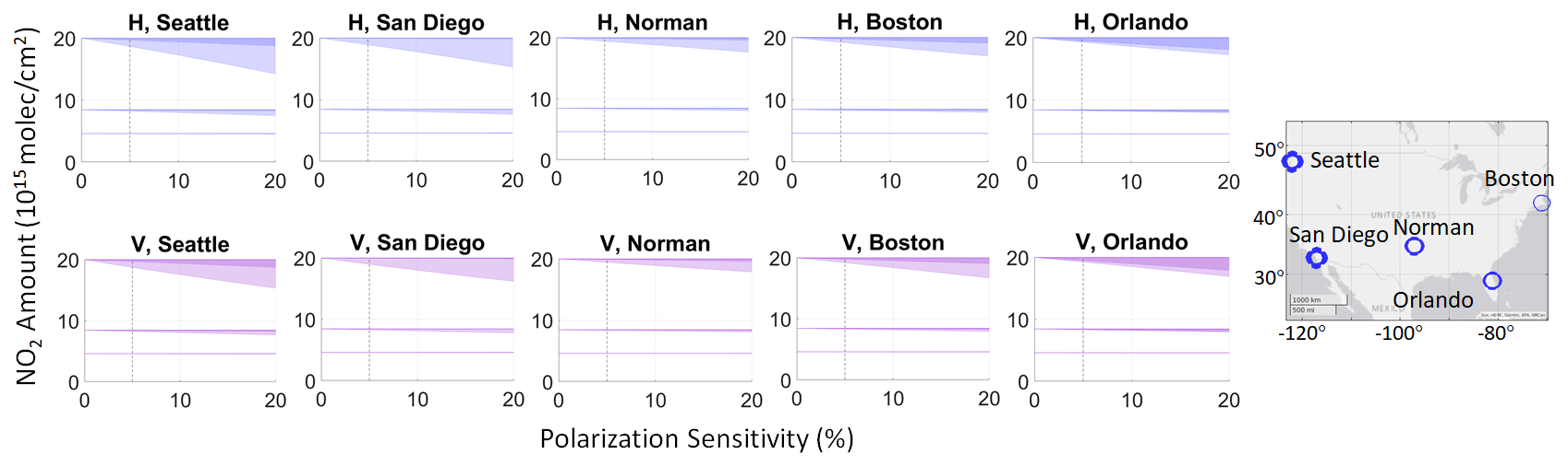
Figure 8 The retrieved amount is shown (left) as a function of polarization sensitivity (PS) for two different orientations (H – horizontal, V – vertical) for selected US locations and NO₂ total vertical amounts: 5.0, 8.6, and 20×10¹⁵ molec. cm⁻². The edge of the darker (lighter) shading shows the retrieved NO₂ amount with a solar zenith angle of 30^∘ (70^∘). The vertical dotted line shows the current PS requirement for reference. The locations are shown (right) on the map, with thicker circles representing higher NO₂ errors (see Table 3, Simulation C for more details.)

In contrast to the previous results with constant profiles across CONUS, Fig. 9 shows the results using GEOS-Chem profiles, which appear qualitatively consistent with the results using the artificial profiles used above (Table 3, Simulation D). The NO₂ amounts for this day, which varied between 2.5 and 6.5×10¹⁵ molec. cm⁻², are displayed. The figure shows the polarization impacts with 5 % PS in the vertical orientation. The impacts are more apparent as the solar zenith angle increases and resemble the previous results in Fig. 7, where the solar zenith angle is fixed at 70^∘. For instance, the NO₂ errors are larger at 20:00 UTC in the eastern regions where the solar angles are relatively large, and the NO₂ errors are larger in the western regions at 16:00 UTC where the solar zenith angles are larger. The higher cloud fraction decreases the retrieval errors, which can be seen in the western regions at 16:00 UTC; although the southwest and southeast have similar solar zenith angles, the southwest has lower retrieval errors due to the increased cloud fraction. As a result of the cloud fraction and lower NO₂ amount, the maximum NO₂ errors found were 0.03×10¹⁵ molec. cm⁻² for this day – a negligible value when compared to the TEMPO precision requirement.

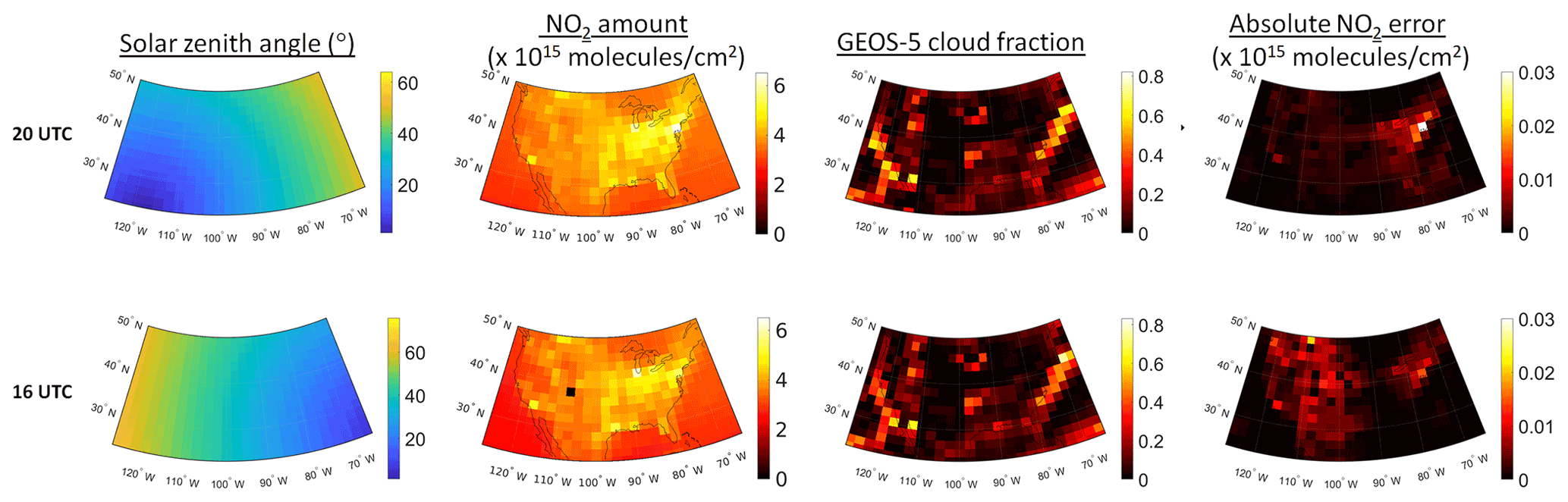
Figure 9 Solar zenith angles, total NO₂ column amount, GOES-5 cloud fraction, and resulting NO₂ errors at 20:00 UTC (top) and 16:00 UTC (bottom). GEOS-Chem NO₂ profiles were used assuming 5% PS with vertical orientation, all water scenes, and clouds at a 2 km altitude (see Table 3, Simulation D for more details.)

4 Summary and conclusions

We demonstrated a simulation and modeling capability to assess polarization effects for ACX predicted performance studies. Our results show that the DOAS spectral fitting step mitigates PS effects in the NO₂ retrieval process. The AMF calculation step, however, can cause retrieval errors from instrument PS when considering partially cloudy scenes. The PS magnitude and orientation (Mueller matrix elements) impacts can cause different NO₂ retrieval errors depending on location, time of day, cloud fraction, and NO₂ amount. For a PS of 5 % with vertical orientation, the maximum NO₂ retrieval errors were 0.25×10¹⁵ molec. cm⁻² for high-pollution cases. In extreme cases, if NO₂ pollution significantly increases to levels on the order of the world's most polluted regions, these errors can reach 1.4×10¹⁵ molec. cm⁻². A more typical maximum error found through analyzing the GEOS-Chem profiles was 0.03×10¹⁵ molec. cm⁻². This study shows that in most cases, the 5 % PS requirement introduces retrieval uncertainties significantly lower than the TEMPO precision requirement except in the most extreme cases. Note that these estimates assume a particular set of instrument Mueller matrix elements. We emphasized a vertical orientation based on an assumed vertical grating orientation for which its polarization axis would likely be in this direction. In this configuration, the instrument effectively sweeps wavelengths over locations in the west–east direction. The Mueller matrix will be updated with the appropriate values as the instrument design matures to refine the estimates of NO₂ retrieval impacts. Our simplified retrieval approach may have neglected factors used in operational retrievals that could be affected by instrument PS and contribute to additional retrieval errors related to estimates of aerosols, surface reflectance, and cloud parameters. Rotational Raman scattering, which has been used in cloud height retrievals (e.g., Vasilkov et al., 2008), for instance, can be particularly sensitive to polarization. Other approaches for cloud height retrievals such as oxygen dimer absorption (Acarreta et al., 2004) should be much less sensitive. We do not account for the PS to cloud height retrievals. The PS to cloud optical thickness is implicitly accounted for within the effective cloud fraction estimation. In addition, the limited set of surface reflectance types that were used as well as the directional and polarization surface effects that were neglected can be included in future work to improve the accuracy of the results. This capability can be utilized to support the development of ACX to continue and build on the legacy of atmospheric composition measurements to forecast and monitor air quality.