the Creative Commons Attribution 4.0 License.
the Creative Commons Attribution 4.0 License.
 | 10 Aug 2022
On the use of high-frequency surface wave oceanographic research radars as bistatic single-frequency oblique ionospheric sounders
Ethan S. Miller
Daniel Cole
Teresa Updyke
We demonstrate that bistatic reception of high-frequency oceanographic radars can be used as single-frequency oblique ionospheric sounders. We develop methods that are agnostic of the software-defined radio system to estimate the group range from the bistatic observations. The group range observations are used to estimate the virtual height and equivalent vertical frequency at the midpoint of the oblique propagation path. Uncertainty estimates of the virtual height and equivalent vertical frequency are presented. We apply this analysis to observations collected from two experiments run at two locations in different years, but utilizing similar software-defined radio data collection systems. In the first experiment, 10 d of data were collected in March 2016 at a site located in Maryland, USA, while the second experiment collected 20 d of data in October 2020 at a site located in South Carolina, USA. In both experiments, three Coastal Oceanographic Dynamics and Applications Radars (CODARs) located along the Virginia and North Carolina coast of the US were bistatically observed at 4.53718 MHz. The virtual height and equivalent virtual frequency were estimated in both experiments and compared with contemporaneous observations from a vertical incident digisonde–ionosonde at Wallops Island, VA, USA. We find good agreement between the oblique CODAR-derived and WP937 digisonde virtual heights. Variations in the virtual height from the CODAR observations and the digisonde are found to be nearly in phase with each other. We conclude from this investigation that observations of oceanographic radar can be used as single-frequency oblique incidence sounders. We discuss applications with respect to investigations of traveling ionospheric disturbances, studies of day-to-day ionospheric variability, and using these observations in data assimilation.
- Article
(5124 KB) - Full-text XML
-
Supplement
(4129 KB) - BibTeX
- EndNote


Understanding the spatial and temporal variations of the ionospheric electron density remains an ongoing challenge in the space weather community. It has been known since the 1950s that disturbances propagate through the ionospheric electron density; these structures have been termed traveling ionospheric disturbances (TIDs) (e.g., Munro, 1950). It has been established that there are two dominant spatial and temporal scales for TIDs: medium-scale TIDs (MSTIDs) and large-scale TIDs (LSTIDs) (Hunsucker, 1982; Hocke and Schlegel, 1996; Harris et al., 2012; Frissell et al., 2014; Otsuka, 2021). However, understanding the physical processes responsible for the generation of these disturbances and understanding the sources of the disturbances are open questions. Some observations have also suggested non-propagating disturbances in the electron density (e.g., Harris et al., 2012).
Making progress toward addressing these questions has been frustrated by relatively sparse observations. In the last 10 years, vertical incidence ionosondes have been used in networks of various spatial sizes (Cervera and Harris, 2014; Reinisch et al., 2018; Belehaki et al., 2020). Incoherent scatter radars provide height-resolved observations, but these facilities are constrained to a single observation location and have a small field of view (Kirchengast et al., 1995, 1996; Nicolls et al., 2004; Nicolls and Heinselman, 2007; Vlasov et al., 2011). SuperDARN has been used to examine TIDs over larger spatial scales, which has produced climatological results particularly for MSTIDs (e.g., Bristow et al., 1994; Frissell et al., 2014). GPS TEC has high spatial density (e.g., Crowley et al., 2016; Coster et al., 2017; Figueiredo et al., 2017), but tends to be strongly influenced by the electron density associated with the F-region peak and the topside of the ionosphere (Nickisch et al., 2016; Belehaki et al., 2020); this technique can be relatively insensitive to the bottom side of the ionosphere.
High-frequency (HF) radio-wave propagation experiments have been developed to understand the electron density of the bottom-side ionosphere. One of the earliest techniques measured the Doppler frequency shift of timing signals (e.g., WWV) that had high phase coherence (Georges, 1968; Crowley and Rodrigues, 2012). Using the Doppler shift, it is possible to derive the ionospheric velocity (Davies, 1990). Chilcote et al. (2015) used a similar technique to measure Doppler shifts of clear-channel AM radio stations in the northeast sector of the US to derive properties of TIDs. TIDs have also been investigated using the frequency and angular sounding (FAS) technique in which observations of angular deflections, the Doppler shift frequency, and the group delay changes are related back to an oscillating mirror disturbance moving through the ionosphere (Beley et al., 1995; Galushko et al., 2003; Paznukhov et al., 2012; Huang et al., 2016). This technique has been primarily used in association with radio telescope observatories (Beley et al., 1995; Obenberger et al., 2019). Recently, the TechTIDE effort has used networks of ionosondes to study TIDs with both vertical incidence and oblique sounding (e.g., Reinisch et al., 2018; Belehaki et al., 2020). In addition, a recent thesis by Heitmann (2020) presents a review of multi-static oblique HF radio-wave propagation used for studies of TIDs.
Over the past 2 decades, advances in receiver technologies and computer storage have evolved to the point that inexpensive, direct-sampling digital software-defined radios are able to sample and store the full 30 MHz HF spectrum. Simultaneously, inexpensive satellite-based precision navigation and timing devices have simplified and reduced the cost of synchronizing stations to produce bistatic observations. These techniques have enabled the development of low-cost, low-power ionosondes at single or multiple frequencies (Vierinen, 2012; Hysell et al., 2016; Saito et al., 2018; Bostan et al., 2019; Chartier et al., 2020). For example, one such experiment has utilized software-defined radios in a network of bistatic HF beacon transmitters and receivers located in Peru that have been used to investigate conditions associated with the development of equatorial spread F (Hysell et al., 2016, 2018, 2021).
One transmission that can be received bistatically is from coastal HF radar stations that are used for ocean wave and current diagnostics within several hundred kilometers of the coastline (e.g., Barrick, 1972; Barrick et al., 1977; Gurgel et al., 1999). These systems operate on the principle of Bragg scatter from ocean waves and operate at a variety of frequencies between 4 and 50 MHz, with some of the most useful frequencies for ionospheric diagnostics operating between 4 and 5 MHz. A typical radar signal at 4–5 MHz has a bandwidth of approximately 25 kHz, which is similar to the current generation of ionosondes (Reinisch, 2021), and a waveform repetition frequency (WRF) of 1 Hz. The modulation is a linear frequency-modulated continuous wave (FMCW) chirp, resulting in a one-way range resolution of ∼ 10–12 km, thus making these transmissions suitable as a single-frequency oblique ionosonde. Although ionospheric sounding has been reported on internet blog posts (RFSPACE, 2011; Estevez, 2017), to our knowledge, there have not been any investigations in the peer-reviewed literature that have evaluated the efficacy of these HF oceanographic radars as potential vertical or oblique single-frequency ionospheric sounders.
The purpose of this investigation is to test whether bistatic observations of coastal HF radars can be used as high-time-resolution single-frequency oblique ionospheric sounders. We present observations of the group range and polarization splitting of the sky-wave mode at two locations using similar software-defined radio systems that observed three Coastal Oceanographic Dynamics and Applications Radar (CODARs) located along the east coast of the US. It is important to note that we are unable to control the frequency or waveform characteristics of the CODAR transmitters, although both factors are known. Using the group range and the known location of the transmitters, we quantify the virtual height and effective vertical frequency using the so-called secant law (Davies, 1990). We compare the CODAR-derived virtual heights and frequency with similar vertical incident HF soundings from the Wallops Island DPS256 digisonde to validate our methodology. We conclude by discussing some of the observed features and their implications for improving understanding of spatial and temporal variations of the electron density in the ionosphere.
2.1 Basic signal processing
A classic “chirped” (linear frequency-modulated) continuous wave (CW) radar operates on the principle of a continuously varying transmitter of known frequency characteristic, for example
where f(t)=κt is a linearly varying frequency. For a monostatic (shared transmit and receive antenna with gain G) radar illuminating targets with radar cross sections (σi) at ranges , the received signal is
Mixing (multiplying) the transmitted signal with the conjugate of the received signal together yields a series of discrete frequency components at baseband corresponding to the ranges to the individual targets.
The range can then be calculated from
This may be generalized to the case of the ionospheric propagation channel between two (bistatic, in the radar lexicon) stations; the “targets” represent individual distinct propagation modes supported by the channel between the two stations. The FMCW radar technique has a number of advantages over pulsed radars, including the higher average power on the target. The Doppler shift is due to a change in phase path to the target,
Practically speaking, the change in the phase path may be calculated by comparing (fitting) the observed phase to subsequent coherently processed pairs (sequences) of returned pulses (waveforms). The WRF sets the Doppler shift aliasing frequency, which is half the WRF.
For the present analysis, a replica of the transmitted waveform is prepared and correlated with the received signal in the frequency domain in the following manner. The replica of a single waveform (pulse) is created, extending Eq. (1) to include a raised-cosine window (w(t)) in order to reduce artifacts when Fourier-transforming a function with finite support:
where κ is the frequency sweep rate and s0 is the magnitude and can be taken as unity. Using discrete sampling, n is the sample index within the waveform.
In order to increase the signal-to-noise ratio and perform Doppler shift calculations, a number (M) of sequential waveforms are integrated coherently. If each waveform contains N samples, this is accomplished in the frequency domain in the following way. The replica is Fourier-transformed and replicated into an N×M matrix:
Likewise, the entire coherent processing interval (CPI, ) is also (discrete) Fourier-transformed (in two dimensions) and the Hadamard (element-wise, ∘) product taken with the replica () to complete the convolution in the frequency domain.
The notation breaks down a bit when we go back to the time domain, where only the Fourier transform in the “fast time” (samples within a waveform) dimension is taken.
The result, , is an N×M matrix that contains the magnitude and phase vs. range (N elements) and Doppler (M elements). Standard range–time–intensity (RTI) presentations of the data may be achieved by identifying or fitting the peak power at each range for each processing interval.
2.2 Virtual height estimation
To determine the virtual height, we make the simple approximation that the ionosphere is effectively a reflecting mirror at an altitude of h, which is defined as the virtual height (Davies, 1990). We determine the virtual height, h, using the following trigonometric relation (Davies, 1990):
where P is the group range, P=cΔt, with Δt being the time delay of the ionospheric channel, and D is the distance between the CODAR transmitter and the receive site. Considering that we obtain the group range, P, and we know the distance D between the transmitter and receiver, this mirror model is the most straightforward model which is consistent with the observables. A more sophisticated treatment of this inversion problem using ray tracing is possible, but our approach is to consider the simplest model first. We assume that the curvature of the Earth is not significant for this application because the ground range is typically less than 600 km (Davies, 1990), but we do use the Haversine formula to calculate the ground distance, D. We also assume that the propagation mode we observe corresponds to the direct sky-wave propagation mode directly from the antenna, and our analysis specifically focuses on one-hop propagation modes vs. multiple hop modes.
We also use the so-called secant law to calculate the equivalent vertical frequency for the oblique propagation path (Davies, 1990),
where fo is the oblique frequency, i.e., the frequency observed at the receiver, and fv corresponds to the vertical frequency of the ionospheric layer at the midpoint of the path between the transmitter and the receiver. The angle ϕ is derived as , where we note that D is known and P is obtained by radar signal processing, as described above in Sect. 2.1.
We use the E region or, when present, the sea surface wave as a means by which to calibrate for an absolute group range for the F-region propagation mode. Each CODAR has a unique time delay set relative to GPS pulse per second (PPS), but those may not be well known ahead of time. The daytime E-region propagation mode is suitable since it occurs at a relatively stable and constant group range. To predict a group range for the E region, , we solve Eq. (10) using the known distance D and an assumed virtual height, hE, of 125 km. We can measure the group range of the E-region hop, , and the calibration time delay, Δ, can be determined as
Our results are relatively insensitive to the choice of hE. This calibration factor can now be used to obtain , where is the measured group range for the F region. Given PF, the virtual height for the F region can be estimated using Eq. (10).
The uncertainty of the virtual height, Δh, can be determined by propagating the uncertainty through Eq. (10),
where Δh is the uncertainty of the virtual height, ΔP is the uncertainty in the group range, and ΔD is the uncertainty in the ground range distance. For this investigation, we assume that ΔD is effectively zero because we know the location of the transmitters and the receiver locations to high levels of certainty. The uncertainty of the group range, ΔP, corresponds to range uncertainty produced by dechirping the waveform. Since the bandwidth of the waveform is ∼25.733913 kHz, the corresponding group range uncertainty is ΔP∼11.7 km (for one-way propagation). The propagated uncertainty for fv is
where D and P are known or observed, respectively.
2.3 Polarization
We also calculated Stokes parameters when we had observations with both loop antennas to determine whether the incoming wave has right-hand or left-hand circular polarization, corresponding to X- and O-mode propagation (in the Northern Hemisphere), respectively. For the convention of increasing phase, the loop antennas define an orthogonal coordinate system,
where Vx and Vy correspond to the complex voltage for the nominal north–south- and east–west-aligned antennas, respectively. Left-hand circular polarization (O mode) corresponds to +V and right-hand circular polarization (X mode) corresponds to −V.
2.4 Group range trace extraction
After performing the radar signal processing, we obtain a time series of the pseudo-group range, in which the time correction has not yet been performed, as discussed above. From a given transmitter, there can be two polarization modes per ionospheric channel. A Python-based “clicker” program was developed and implemented to extract the pseudo-group range time series for each ionospheric propagation mode and polarization. Although more sophisticated methods could be used, including cluster algorithms or machine learning techniques, we find that this problem is well suited to a more manual approach, similar to hand-scaling ionograms (Dandenault et al., 2020).
The signal processing outlined in Sect. 2 is agnostic to the software-defined radio data acquisition system; therefore, a wide variety of experiments can be envisioned and conducted. Table 1 describes the cost breakdown of the software-defined radio system used at the Clemson Atmospheric Research Laboratory (hereafter referred to as “CARL”) site, including the receive antennas but excluding the cost of a host computer. Both systems at both receive locations, as discussed below, are based on a commercially available Ettus Research Universal Software Radio Peripheral (USRP) model N210, which provides complex baseband samples over a simple Ethernet interface and a well-defined API. The standard build of the FPGA in the USRP N210 allows IQ sampling at a minimum of 250 kHz, which is then filtered and decimated in real time by a factor of 8 in software on a personal computer and recorded to disk. These raw, decimated IQ samples are processed offline using the algorithm described previously. Other software-defined radios could provide similar performance to the Ettus USRP system, but such an investigation is outside the scope of this paper.
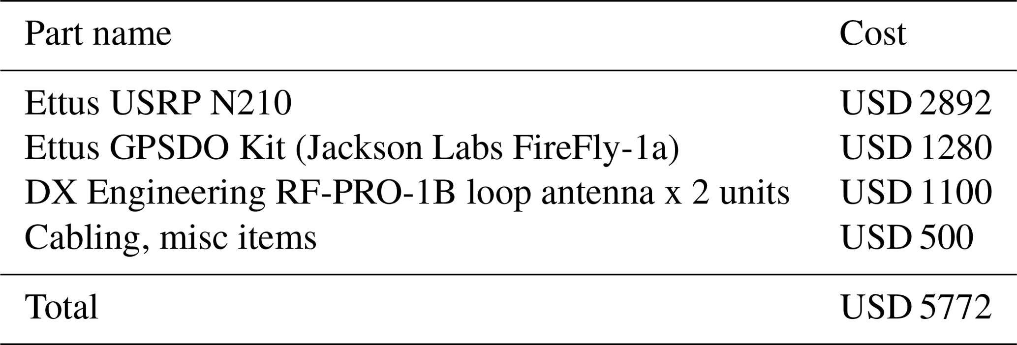
The USRP N210 is synchronized to GPS PPS and a stable 10 MHz time base either via external inputs or an internal option GPS disciplined oscillator (GPSDO) board (Jackson Labs FireFly-1a). Recordings start on the rise of a 1 PPS pulse and continue for the duration of the coherent processing interval, usually 5–20 s. Besides bistatic time synchronization, the GPSDO also provides clock stability, which is essential for performing the signal processing described in Sect. 2.1. The oscillator native in the USRP N210 has a stability of 2.5 ppm, which is insufficient for this application because the dechirped waveform will have large range resolution driven by the jitter of the oscillator. The USRP is designed to be a component in a receiving system and therefore requires a front-end low-noise amplifier to increase gain and reduce noise figure, even at HF. A suitable amplifier has about 20 dB of gain and a moderately high (>20 dBm) power at 1 dB compression.
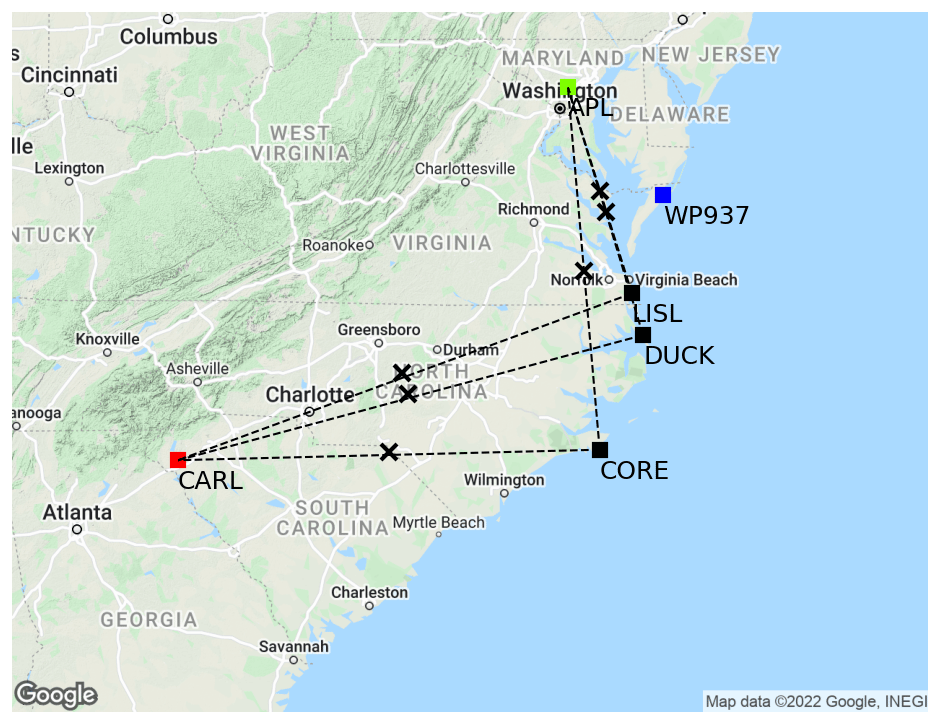
Figure 1A map showing the physical locations of the CODAR transmitters (DUCK, CORE, and LISL), the Wallops Island digisonde (WP937), and the receive locations of MSR and CARL. Midpoint locations along the great circle path are shown as black X marks.
We present results collected at two locations in different years, but using similar data collection systems. A quiet, exurban receiving site (hereafter referred to as “MSR”) was established near the Johns Hopkins University Applied Physics Laboratory at approximately 39.34∘ N, 77.06∘ W. A short, commercially available “active whip” (electric field probe) antenna about 2 m tall was installed at ground level. The receiver was tuned to 4.53718 MHz; three CODAR radars along the Virginia and North Carolina coast share the same frequency allocation by a time-division multiple-access (TDMA) scheme, with each radar's chirp start time-delayed by some arbitrary number of milliseconds from GPS PPS. These CODAR transmitters have station code names DUCK, LISL, and CORE. The second location was at the Clemson Atmospheric Research Laboratory (CARL). Two crossed-loop antennas were used at this location, and the 4.53718 MHz CODAR band was also monitored.
Figure 1 shows a map detailing the locations of CARL and MSR relative to the CODAR transmitters and a diagnostic ionosonde, i.e., a DPS256 digisonde, at the NASA Wallops Flight Facility (hereafter referred to by its call sign “WP937”). The midpoints of the ionospheric channel from MSR to the CODARs are indicated by black X marks. The midpoints for the CODAR–CARL path form a north–south line located in North Carolina. The locations of the receiver, transmitters, and diagnostic instrument are summarized in Table 2.

The results presented correspond to 10 d of continuous data collected at the MSR site during 10–19 March 2016 and 20 d of continuous data collected at the CARL site for 5–24 October 2020. Results are shown from two locations to demonstrate that similar data collection systems produce consistent features. A representative example from 10 March 2016 at MSR and 8 October 2020 at CARL is presented in Figs. 2 and 3, respectively. These figures correspond to pseudo-group range–time–intensity (RTI) on the y–x–z axis, respectively. The circuits are arranged in the following order from the smallest GPS PPS delay to the largest: LISL, DUCK, and CORE. This arrangement is based on an internal time offset from GPS PPS, which has been provided by the Radiowave Operators Working Group.
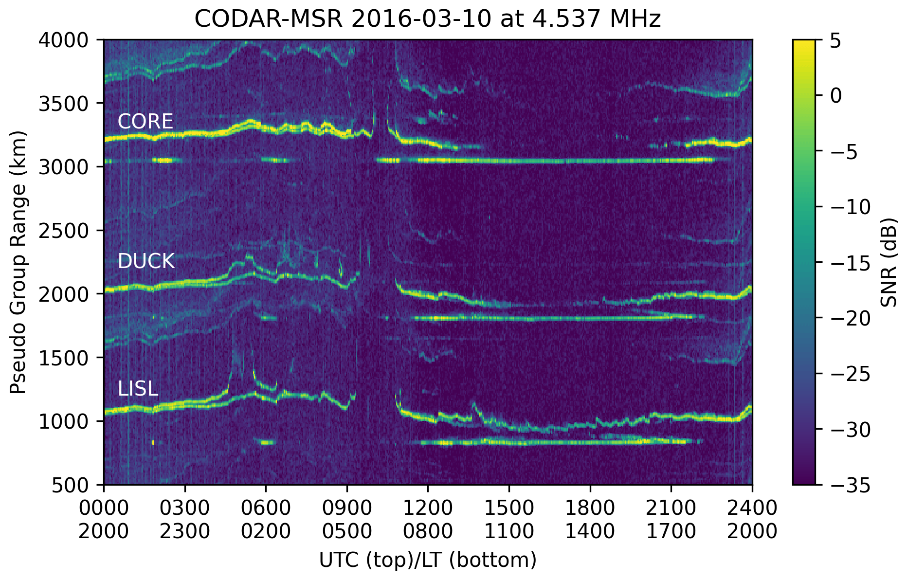
Figure 2A 24 h (pseudo) range–time–intensity (RTI) plot from three ocean wave radar transmitters received at MSR at 4.53718 MHz on 10 March 2016. The pseudo-group ranges corresponding to the LISL, DUCK, and CORE CODAR transmitters are listed. The figures are plotted with respect to UTC, but Eastern Time (LT) is also shown for reference. See the text for further discussion.
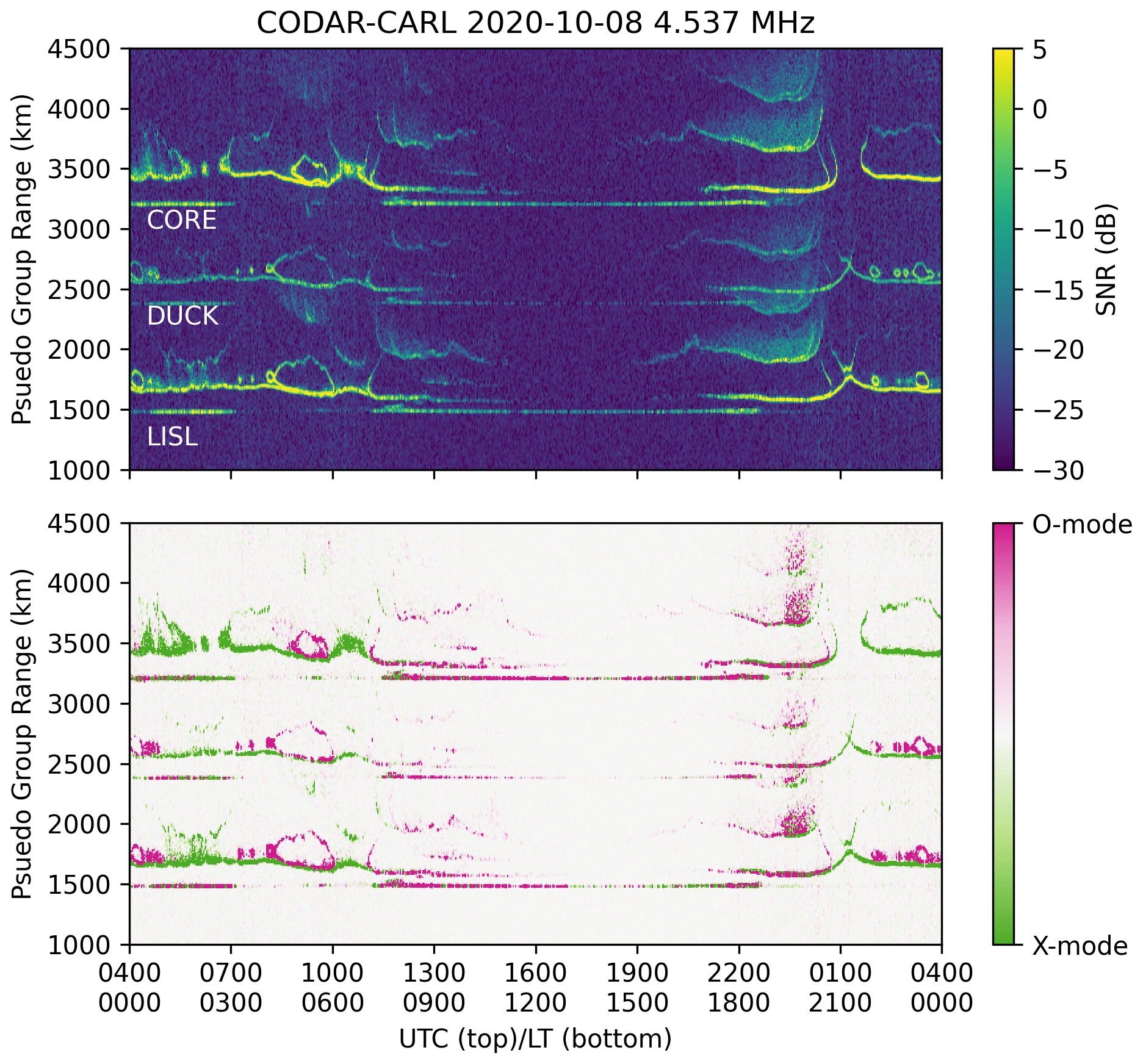
Figure 3Top row: 24 h (pseudo) range–time–intensity plot from three North Carolina CODAR transmitters received at CARL at 4.53718 MHz on 8 October 2020. Bottom row: polarization separation of O- and X-mode propagation as purple and green, respectively. See the text for further discussion.
A few features are quite clear in Fig. 2. Universal Time (UTC) is local time +4 h; so, the time series begins in the early evening local time, a little after sunset. We note that even though a single antenna was used, mode splitting becomes apparent in the pseudo-group range, as indicated by two distinct propagation modes at the same time. Throughout the night, 00:00–11:00 UTC, two stable F-region propagation modes are present, separating slowly in range as the bottom side of the F region erodes due to recombination. Around 04:30 UTC on the LISL circuit, the ordinary (O) mode begins to penetrate through the ionosphere before returning at 05:30 UTC for another hour. After about 06:30 UTC, only the extraordinary (X) mode completes the circuit until it disappears at 09:30 UTC. On the DUCK circuit, the O mode departs from the X mode by 100–200 km during 04:30–05:30 UTC and after 06:30 UTC but does not penetrate the ionosphere as in the LISL case. This is due to the slightly longer great circle distance to DUCK and attendant increase in the subionospheric zenith angle. Likewise, the O mode remains subionospheric until 09:30 UTC on the CORE circuit.
Also during the night of 10 March 2016, several sporadic E layers appear at around 02:00–03:00 and 05:30–07:00 UTC. We also note that between 18:00 and 22:00 UTC the DUCK and LISL link shows evidence of a descending layer. For the sake of discussion, assume that the geographic extent of the sporadic E layers covers the reflection points of all three circuits (in this case, a north–south extent of about 70 km); we observe the appearance and dissipation at different probing critical frequencies. By solving Eq. (11) this expression for fv with fMUF=4.53718 MHz yields the “cutoff frequency” for each circuit in the E region. That is, Eq. (11) predicts the ionospheric critical frequency at which the fixed-frequency circuit closes; i.e., the propagation is no longer supported on the circuit. Since each circuit has a different great circle distance (and therefore subionospheric zenith angle), it creates a sieve to investigate the rate of change in electron density.
The top row of Fig. 3 shows a similar RTI as Fig. 2 using the data collection system at CARL. We find many similar features between the observations from MSR and the observations from CARL. For example, a stable daytime E region due to solar production becomes clear between 10:30 and 22:30 UTC at pseudo-group ranges of 1500, 2300, and 3600 km, respectively. D-region absorption is also evident during the day, as represented by the fading of the F2 path or closing of the propagation circuit during the daytime. Dawn and dusk show rapid changes in the pseudo-group range, which occur at approximately 10:30 UTC and near 01:00 UTC, respectively. These rapid changes correspond to an increase and decrease in photoionization caused by the sun rising and setting locally, respectively.
Between 21:00 and 01:00 UTC, there are signatures of multipath propagation and range spreading. In the case of CORE and LISL, there are three identifiable propagation paths. The range spreading signature could be associated with ground scatter, sea backscatter, or in some cases (not currently presented) signatures of midlatitude spread F, which we may also expect to appear in the one-hop propagation modes as well. The focus of this investigation is on the one-hop sky-wave propagation, and therefore investigation of these multipath signatures is left for a future investigation.
The bottom row of Fig. 3 presents the polarization calculated from the cross-loop antenna configuration at CARL using Eq. (15). The polarization provides additional insight into the propagation modes that were observed with the system at CARL. We find at night, between 00:00 and 10:30 UTC and after 01:00 UTC, that the X mode is the dominant propagation mode. For this day, we also find some intervals in which both O- and X-mode propagation were present including between 07:00 and 10:00 UTC. During this interval in particular, the ionosphere may have been supporting a high and low ray configuration (Davies, 1990) in the O-mode propagation, which corresponds to the “hoop” feature in the pseudo-group range. However, further investigation is required to verify this hypothesis, which is outside the scope of the current investigation.
4.1 Comparison with Wallops Island digisonde
Figure 4 presents a comparison of 5 d of virtual heights derived from CODAR observations relative to virtual height observations provided by the Wallops Island digisonde, WP937. The 5 d chosen correspond to 15–19 October 2020. For each CODAR–CARL circuit, the corresponding virtual height was calculated using Eq. (10), and the equivalent vertical frequency, fv, was calculated using Eq. (11) above. We interpret the location of the virtual height and equivalent vertical frequency to correspond to the midpoint of the great circle path between the CODAR transmitter and CARL, as shown as black X marks in Fig. 1. From the digisonde data, we extract the virtual heights for the frequency nearest to the equivalent vertical frequency derived from the CODAR observations. We plot the power from this frequency slice as a function of time, similar to the height–time–intensity figures discussed in Altadill et al. (2019). For the digisonde data, we consider both polarizations, with O- and X-mode corresponding to purple and green, respectively, but we excluded the received power that is <30 dB below the peak power. The black triangles and blue dots correspond to the virtual height for the X- and O-mode CODAR–CARL paths, respectively. This digisonde processing creates an equivalent single-frequency time series, which is shown in the top three rows for LISL, DUCK, and CORE, respectively. The fourth row shows the equivalent vertical frequency derived for the X mode for LISL, DUCK, and CORE as green dots, orange squares, and purple triangles, respectively; the fifth row shows the equivalent vertical frequency derived for the O mode.
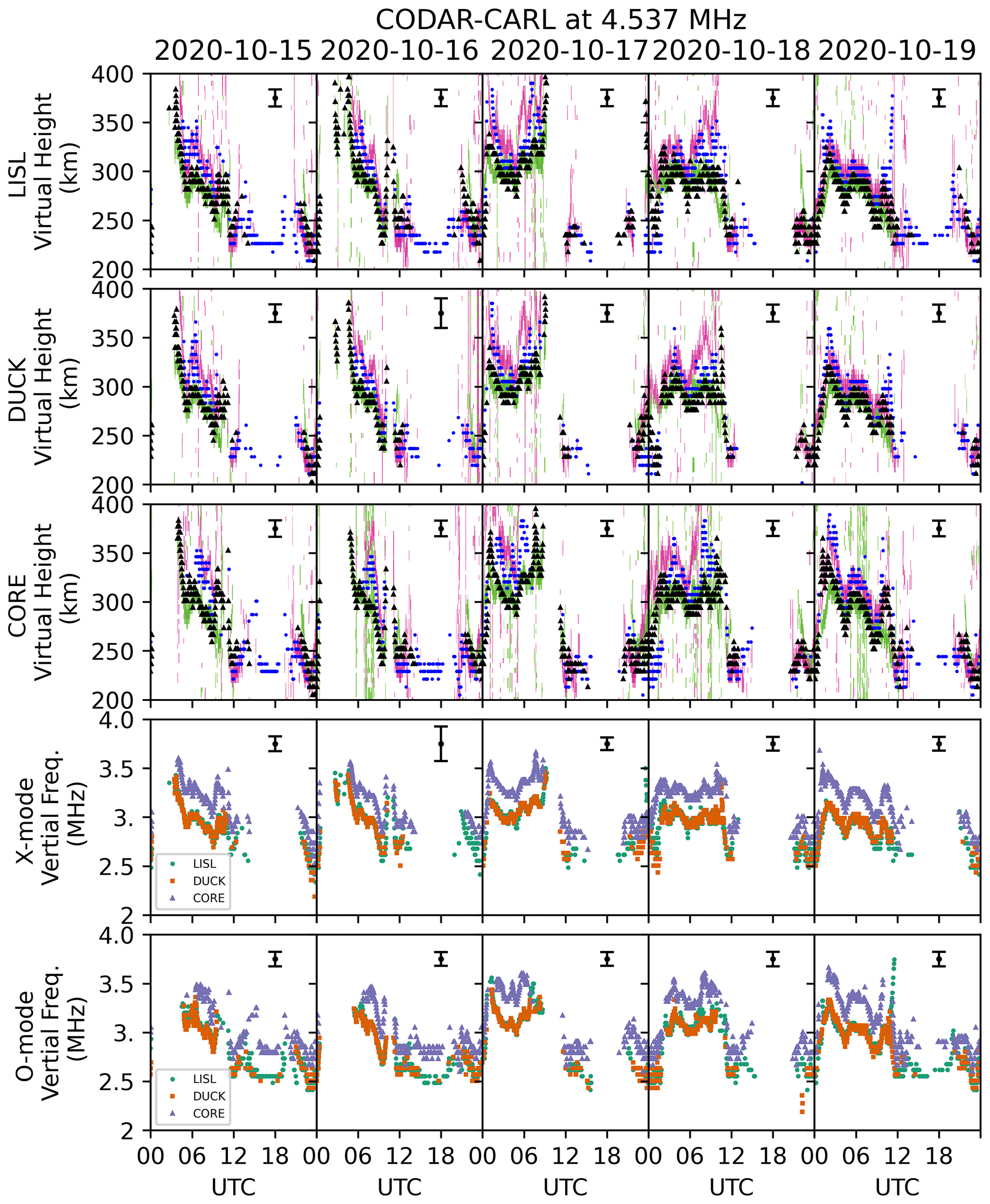
Figure 4A virtual height–time derived using the oblique CODAR–CARL observations vs. the WP397 digisonde at Wallops Island, VA, between 15 and 19 October 2020. In the top three rows, the X- and O-mode virtual height time series are plotted as black triangles and blue dots, respectively. The WP937 X mode and O mode at the frequency nearest to the equivalent vertical frequency derived using the CODAR observations are shown as green and purple, respectively. From top to bottom, rows 1–3 show the virtual height calculated from the LISL, DUCK, and CORE CODARs. The error bar plotted at 18:00 UTC is the maximum propagated uncertain estimated, calculated using Eq. (13). Rows 4 and 5 show the vertical frequency calculated using the secant law in Eq. (11) for the X and O mode, respectively. More details can be found in the text.
We find good agreement between the oblique CODAR-derived virtual height and virtual height from the WP937 digisonde. The consistency between the CODAR observations and the WP937 observations is best during the night, between roughly 01:00 and 10:30 UTC. We observe a gap in the CODAR observations during the day from 10:30–22:30 UTC, which is due primarily to absorption associated with the daytime D-region ionosphere. The propagation channel between the CODAR transmitter and CARL is closed. Additional gaps in data sometimes correspond to the ionosphere not supporting propagation; for example, between ∼ 00:00 and 06:00 UTC on 16 October 2020, the original RTIs show a closed propagation channel during the night.
Figure 5 corresponds to 5 d of observations from MSR between 10 and 14 March 2016, looking at the same CODAR transmitters at 4.53718 MHz and presented in a similar format as Fig. 4. In this case, because a single vertical antenna was used we present only a single virtual height, although there was propagation mode splitting evident in the pseudo-group range, as shown above. We find good agreement when comparing the virtual height from WP937 with the equivalent virtual height from the CODAR observations. The nighttime sector, 00:00–09:00 UTC, is well resolved with these observations and there are fairly consistent features day to day for this 5 d interval. We also find that the daytime F-region ionosphere can be resolved, in particular for the LISL circuit between 12:00 and 18:00 UTC. For the case of MSR, LISL has the shortest circuit length; therefore, we expect the equivalent vertical frequency to be the largest. The equivalent vertical frequencies, presented in the bottom row, are nearest to the transmitter frequency, as indicated by the secant law in Eq. (11) above. With this analysis, the spatial diversity of transmitters relative to receivers also provides frequency diversity.
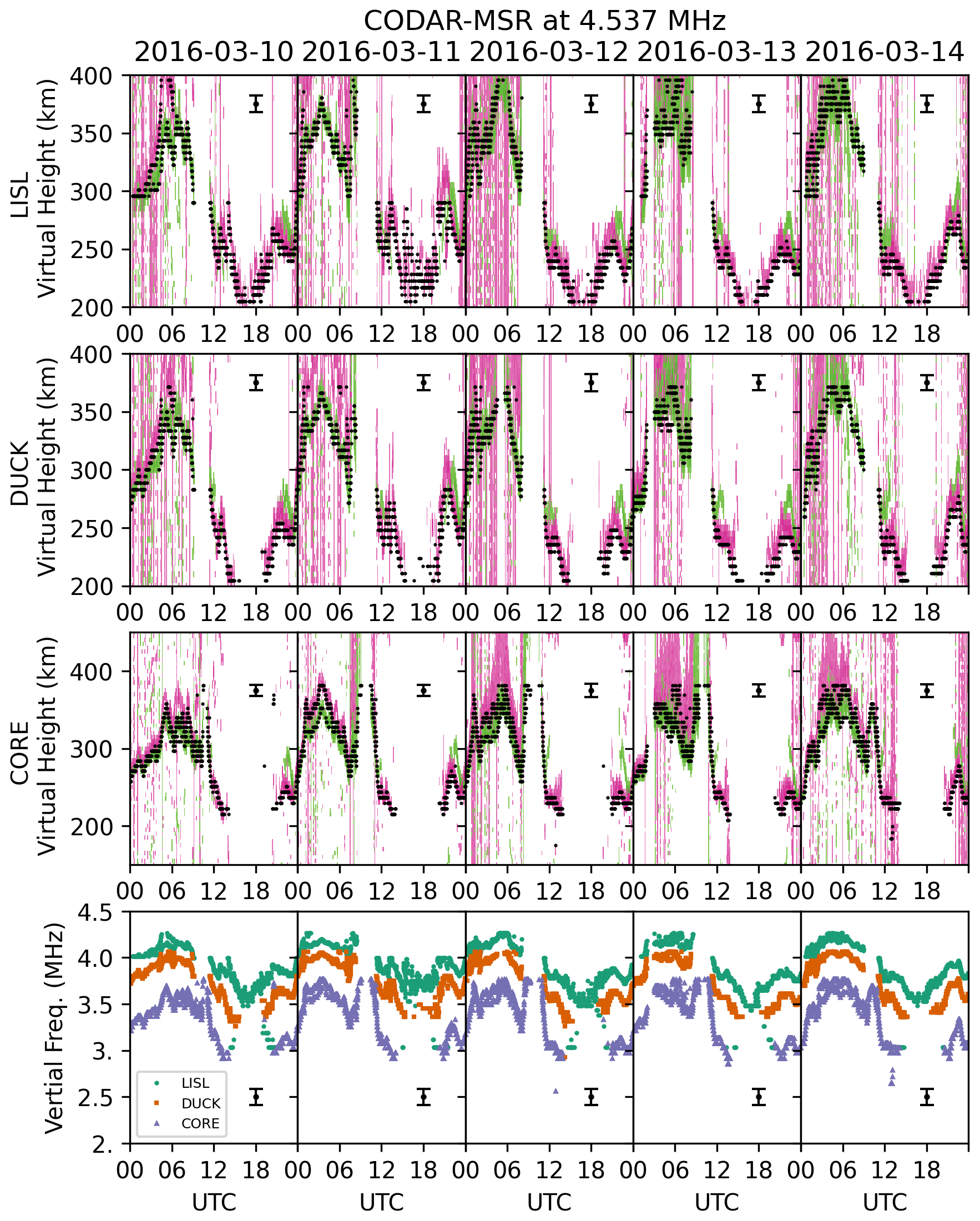
Figure 5A comparison of the virtual heights derived using the CODAR observations from MSR for 10–14 March 2016 and the virtual height from the WP937 digisonde at Wallops Island, VA. The figure is in the same format as Fig. 4, except there is no distinction between the X and O mode for the CODAR observations. See the text for more details.
The virtual height separation between the X and O mode is less pronounced for the CODAR observations from the CARL site vs. the digisonde observations or the from the MSR site. This can be partially attributed to oblique propagation. The propagation delay time (group range) will tend to increase because the ray will slow down as it nears the reflection point. However, as the ray paths become more oblique, the rays will tend to reflect at lower altitudes, thus resulting in a similar group range between the X- and O-mode propagation.
For completeness, we include observations from CARL for 5–9, 10–14, and 20–24 October as Figs. S1, S2, and S3 in the Supplement, respectively. Observations from MSR are included for 15–19 March as Fig. S4.
Our results have demonstrated that coastal HF surface wave radars, with appropriate waveforms, can be used as bistatic oblique ionospheric sounders at a single frequency. The RTIs shown in Sect. 4 are qualitatively consistent with Fig. 2 in Hysell et al. (2016), which illustrates the results from an HF beacon experiment that uses a pseudo-random code with 10 µs baud length, and Fig. 5 from Bostan et al. (2019). Our analysis demonstrates that a time series of the virtual height can be obtained through bistatic reception of CODAR transmissions, and our observations produce similar virtual height as that extracted from the WP937 digisonde observations at a single frequency.
5.1 Applications
Observations such as these can be used to understand the spatial scale sizes of disturbances that affect the bottom-side electron density. These disturbances may include propagating disturbances, i.e., TIDs, or non-traveling disturbances, which can have scale sizes less than 500 km (Harris et al., 2012). The spatial distribution of north–south CODAR–receiver midpoints can enable investigations to test whether these disturbances are propagating. We would expect to see a time delay between the digisonde observations of virtual height relative to the CODAR observations of virtual height or between virtual height observations derived solely from multiple CODAR observations. Although it is important to note that while CODAR observations in the 4 MHz band have a minimum sweep period of 1 s, a full digisonde sweep is of the order of 5 min. If, hypothetically, the CODAR midpoint relative to a digisonde were separated by ∼200 km (∼2∘ latitude), for an LSTID, with a nominal propagation speed of 500 m s−1 purely north–south (e.g., Figueiredo et al., 2017), the time delay would be ∼6 min. This time interval is resolvable by CODAR observations alone with ≤1 min sampling, but approximately 1–2 data points of digisonde observations would cover the passage of a wavefront of the LSTID at a fixed frequency due to the ∼5 min revisit time.
Figure 6 presents an example of virtual height observations of an assumed TID observed on 6 October 2020 between 00:00 and 12:00 UTC during local night. We find perturbations in the virtual height derived using CODAR data that are in phase with virtual height observations derived from the WP937 digisonde for the same frequency. Figure 6 shows that the CODAR-derived virtual height tracks the WP937 X-mode time series very well. Previous ionosonde observations have shown that TIDs cause perturbations of isodensity contours that are in phase as the ionosonde frequency increases (e.g., Reinisch et al., 2018; Altadill et al., 2019; Belehaki et al., 2020). Our observations are consistent with TechTIDE height–time–intensity (see Fig. 6, Altadill et al., 2019).
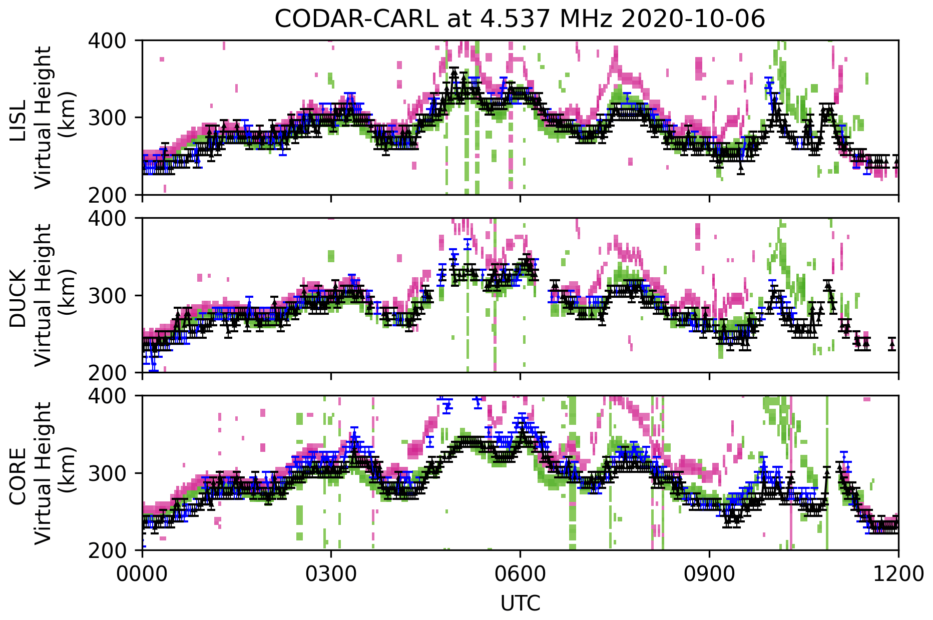
Figure 6An example of virtual height observations of an assumed TID on 6 October 2020 from 00:00–12:00 UTC. The format is similar to the top three rows of Fig. 4. The virtual height derived from CODAR observations for the X and O mode are shown as black triangles and blue dots, respectively. We also show uncertainty estimates for the virtual height. More details can be found in the text.
The implications of a small time delay may suggest a preferential propagation direction; i.e., a crest of the TID may be over both the Wallops digisonde WP937 and the midpoints of the CODAR at the same time. Another possible explanation is that the ionosphere was moving upward and downward over a spatially extended region that covers the CODAR midpoints and WP937. Either of these hypotheses can be investigated further with additional CODAR observations and ionosonde observations, but this investigation is outside the scope of this paper. Additional data sources, such as GPS TEC or airglow imagers, may be able to provide added insight into these structures. The observations from HF coastal radars could be used as an additional signal source for TechTIDE or other similar efforts to understand and mitigate effects from TIDs.
Nearly continuous bistatic observations can be used to quantify the day-to-day variability of the bottom-side ionosphere. TIDs are one of the most significant sources of day-to-day variability (e.g., Harris et al., 2012; Frissell et al., 2014; Reinisch et al., 2018). A recent investigation by Zawdie et al. (2020) examined bottom-side day-to-day variability using the SAMI-3/WACCM coupled ionosphere–thermosphere model and comparing the model output with ionosonde observations. They concluded that one of the best parameters to quantify day-to-day variability are virtual height measurements at a fixed frequency, which this investigation has demonstrated can be produced from bistatic reception of the CODAR transmissions. Qualitatively, Zawdie et al. (2020) suggested there was more variability during the local nighttime sector, which is consistent with the observations in this investigation. CODAR-derived virtual heights can be used to assess day-to-day variability, although limited to a narrow range of frequencies, but with higher time resolution and more diverse spatial coverage.
A third application is use of these data in assimilative ionosphere models of the bottom-side ionosphere. A number of recent investigations have suggested methodologies to assimilate data collected from HF beacons to inform regional ionosphere models (Nickisch et al., 2016; Fridman et al., 2016; Mitchell et al., 2017; Hysell et al., 2016, 2018; Munton et al., 2019; Hysell et al., 2021). Our simple analysis illustrates the potential efficacy of high-bandwidth FMCW transmitters as a possible data source for these models. Additionally, these observations provide a suitable source to examine other propagation models, including the effects of TIDs (Huang et al., 2016; Zawdie et al., 2016; Psiaki, 2019).
5.2 Limitations and advantages
One of the key limitations of passive reception of single-frequency sounding is limited probing of the ionospheric plasma. Recall that we do not have control over the transmitter frequency, schedule, or waveform characteristics. Clearly, a swept frequency vertical incidence sounder is able to probe the bottom-side altitude distribution of the ionospheric electron density, while the single-frequency sounding method is limited to a smaller range of electron densities. From the secant law in Eq. (11) above, the equivalent vertical electron density that can be probed cannot be greater than the transmit frequency of the CODAR. This limits our observations to 4.5 MHz for the case of a nearly vertical incident sounding. As the distance between the transmitter and receiver increases the equivalent vertical frequency will also decrease. One way to circumvent this issue would be to use additional frequencies, as has been done in the investigation by Chartier et al. (2020).
A few other limitations include degraded signal performance during the daytime due to D-region absorption. Second, the unambiguous Doppler resolution is approximately 0.5 Hz for a 1 s FMCW signal. Pulsed-Doppler signal processing techniques can be applied (Richards, 2005); this step is left for a future investigation.
While there are some important limitations with this technique, there are also some advantages that make use of these signals appealing. First, our results demonstrate additional use of an existing network of coastal surface wave HF transmitters; therefore, funding for a transmitter is not required. Second, the overall cost of the system is relatively inexpensive and with advances in software-defined radio technology, particularly with respect to clock stability, it is likely that the system cost will continue to decrease over time. In fact, it is possible that the current-generation software-defined radio dongles with a 0.5 ppm temperature-controlled crystal oscillator (TCXO) may be used for this application. Third, the spatial distribution of stations can be configured to more optimally probe the ionospheric isodensity. For the first-order analysis we have performed, the controlling factor of the equivalent vertical electron density is the distance from the CODAR transmitter to the receiver. Fourth, the data we obtain has high temporal resolution. In principle, we could obtain a data point at 1 s cadence, which is significantly faster than a typical frequency sweep of an ionosonde corresponding to 5–15 min depending on the sweep rate. Finally, what is presented in this investigation only shows use of polarization and group range data. Other state parameters can be obtained, including angle of arrival and Doppler shift, which can be used in a more rigorous estimation of the ionospheric electron density as has been performed in other investigations (Galushko et al., 2003; Paznukhov et al., 2012; Huang et al., 2016; Hysell et al., 2018, 2021).
We present an investigation demonstrating that bistatic observations of existing high-frequency coastal oceanographic radars, with suitable waveform characteristics, can be used as single-frequency oblique ionospheric sounders, even though we do not have control over the transmitter frequency or waveform characteristics. The techniques we describe in this investigation are agnostic of the type of software-defined radio system used, although good frequency stability is required. We present techniques for extracting the group range from the bistatic observations and using the E region as a means to provide an absolute time delay for the F-region propagation mode. The virtual height and equivalent vertical frequency at the midpoint of the oblique path are also estimated using the group delay observations and the known location of the transmitters and receivers. Uncertainty estimates of the virtual height and equivalent vertical frequency are also derived.
We performed an experiment in which we collected 10 d of data in March 2016 from a site in Maryland, USA (MSR), and 20 d of data collected in October 2020 from a site near Clemson, South Carolina, USA (CARL). For both experiments, we used a similar hardware setup utilizing an Ettus USRP N210 software-defined radio, including the GPSDO unit. We obtained bistatic observations of Coastal Ocean Dynamics Applications Radars (CODARs). Our observations for both intervals focused on one frequency band at 4.53718 MHz, which included three CODAR transmitters located on the US east coast with station names DUCK, CORE, and LISL. The digisonde located at Wallops Island, VA (WP937), was used as the diagnostic to compare and validate the observations collected from oblique CODAR–MSR(CARL) propagation channels.
For the analysis, we estimated the virtual height and equivalent vertical frequency for the CODAR–MSR(CARL) path. For the digisonde data, we extracted the virtual height at the frequency nearest to the CODAR-derived equivalent vertical frequency and produced a time series of the virtual height of the digisonde data. Upward or downward virtual height changes observed by the digisonde were also observed by the CODAR-derived observations with small time delays. The agreement was best during the night, which was partially attributed to significant D-region absorption during the day, thus resulting in no suitable CODAR–CARL path. Our results show that disturbances in the virtual height appear to be correlated over a spatial scale length of ∼350 km.
To our knowledge, this is one of the first investigations that has compared and validated bistatic HF observations from oceanographic radars with ionosonde measurements. The application of this investigation may be useful for expanding spatial coverage for traveling ionospheric disturbance studies, day-to-day variability studies, or within data assimilation routines. Additionally, HF coastal radars may be used by the scientific community or radio amateurs, i.e., HamSci, as a suitable RF source for ionospheric sounding.
Processed and analyzed CODAR observations from CARL and MSR that were used in this investigation can be found at https://doi.org/10.5281/zenodo.6341875 (Kaeppler and Miller, 2022). The Wallops Island digisonde data for October 2020 can be found at https://data.ngdc.noaa.gov/instruments/remote-sensing/active/profilers-sounders/ionosonde/mids12/WP937/individual/ (last access: 1 August 2022, National Geophysical Data Center, 2021a) and for March 2016 at https://data.ngdc.noaa.gov/instruments/remote-sensing/active/profilers-sounders/ionosonde/mids08/WP937/individual/ (last access: 1 August 2022, National Geophysical Data Center, 2021b). The dgsraw used to process the digisonde data is publicly available at https://data.ngdc.noaa.gov/instruments/remote-sensing/active/profilers-sounders/ionosonde/software/Digisonde/ (last access: 26 July 2022, NOAA National Centers for Environmental Information, 2022). Ionosonde data as part of the Global Ionospheric Radio Observatory (GIRO) are available at https://doi.org/10.5047/eps.2011.03.001 (Reinisch and Galkin, 2011).
The supplement related to this article is available online at: https://doi.org/10.5194/amt-15-4531-2022-supplement.
SRK collected and analyzed data from CARL and MSR, produced figures, and drafted the paper. ESM provided CODAR observations from the MSR site and drafted portions of the paper. DC developed the Python pseudo-range extraction algorithm and applied it to the CARL dataset. TU provided timing information for the CODARs located along the east coast of the US.
The contact author has declared that none of the authors has any competing interests.
Publisher's note: Copernicus Publications remains neutral with regard to jurisdictional claims in published maps and institutional affiliations.
Stephen R. Kaeppler wishes to acknowledge Gary Bust for useful contributions to this paper. Ethan S. Miller acknowledges fruitful discussions with Vito Mecca and Greg Ginet of MIT Lincoln Laboratory. The LISL transmitter is operated by Teresa Updyke at Old Dominion University as part of the Mid-Atlantic Regional Association Coastal Ocean Observing System (MARACOOS). The DUCK and CORE transmitters are operated by University of North Carolina, East Carolina University, and Coastal Studies Institute personnel through the Southeast Coastal Ocean Observing Regional Association (SECOORA). We wish to thank Terrance Bullett for writing the dgsraw, which was used to process the digisonde data, and Lowell Digisonde for collecting ionosonde data as part of the Global Ionospheric Radio Observatory (GIRO).
Stephen R. Kaeppler was supported by the Office of Naval Research (grant no. N00014-21-1-2546) with a grant to Clemson University. Daniel Cole was supported by an Undergraduate Student Research Award provided by the NASA South Carolina Space Grant Consortium. Ethan S. Miller was supported by the Air Force Office of Scientific Research (grant no. FA9550-14-1-0278) through an Office of Naval Research (grant no. N00014-17-1-2123) grant to JHU/APL. The the Mid-Atlantic Regional Association Coastal Ocean Observing System (MARACOOS) is supported with funding provided by the National Oceanic and Atmospheric Administration (award contract NA16NOS0120020).
This paper was edited by Jorge Luis Chau and reviewed by David Holdsworth and one anonymous referee.
Altadill, F., Belehaki, A., Blanch, E., Borries, C., Buresova, D., Chum, J., Galkin, I., Haralambus, H., Juan Zornoza, J. M., Kutiev, I., Oikonomou, C., Sanz Subirana, J., Segarra, A., and Tsagouri, I.: Report on the design and specifications of the TID algorithms and products, Zenodo, https://doi.org/10.5281/zenodo.2590419, 2019. a, b, c
Barrick, D.: Remote sensing of sea state by radar, in: Ocean 72 – IEEE International Conference on Engineering in the Ocean Environment, Newport RI, USA, 13–15 September 1972, IEEE, 186–192, https://doi.org/10.1109/OCEANS.1972.1161190, 1972. a
Barrick, D. E., Evans, M. W., and Weber, B. L.: Ocean Surface Currents Mapped by Radar, Science, 198, 138–144, https://doi.org/10.1126/science.198.4313.138, 1977. a
Belehaki, A., Tsagouri, I., Altadill, D., Blanch, E., Borries, C., Buresova, D., Chum, J., Galkin, I., Juan, J. M., Segarra, A., Timoté, C. C., Tziotziou, K., Verhulst, T. G. W., and Watermann, J.: An overview of methodologies for real-time detection, characterisation and tracking of traveling ionospheric disturbances developed in the TechTIDE project, J. Space Weather Spa., 10, 42, https://doi.org/10.1051/swsc/2020043, 2020. a, b, c, d
Beley, V. S., Galushko, V. G., and Yampolski, Y. M.: Traveling ionospheric disturbance diagnostics using HF signal trajectory parameter variations, Radio Sci., 30, 1739–1752, https://doi.org/10.1029/95RS01992, 1995. a, b
Bostan, S. M., Urbina, J. V., Mathews, J. D., Bilén, S. G., and Breakall, J. K.: An HF Software-Defined Radar to Study the Ionosphere, Radio Sci., 54, 839–849, https://doi.org/10.1029/2018RS006773, 2019. a, b
Bristow, W. A., Greenwald, R. A., and Samson, J. C.: Identification of high-latitude acoustic gravity wave sources using the Goose Bay HF Radar, J. Geophys. Res., 99, 319–331, https://doi.org/10.1029/93JA01470, 1994. a
Cervera, M. A. and Harris, T. J.: Modeling ionospheric disturbance features in quasi-vertically incident ionograms using 3-D magnetoionic ray tracing and atmospheric gravity waves, J. Geophys. Res.-Space, 119, 431–440, https://doi.org/10.1002/2013JA019247, 2014. a
Chartier, A. T., Vierinen, J., and Jee, G.: First observations of the McMurdo–South Pole oblique ionospheric HF channel, Atmos. Meas. Tech., 13, 3023–3031, https://doi.org/10.5194/amt-13-3023-2020, 2020. a, b
Chilcote, M., LaBelle, J., Lind, F. D., Coster, A. J., Miller, E. S., Galkin, I. A., and Weatherwax, A. T.: Detection of traveling ionospheric disturbances by medium-frequency Doppler sounding using AM radio transmissions, Radio Sci., 50, 249–263, https://doi.org/10.1002/2014RS005617, 2015. a
Coster, A. J., Goncharenko, L., Zhang, S.-R., Erickson, P. J., Rideout, W., and Vierinen, J.: GNSS Observations of Ionospheric Variations During the 21 August 2017 Solar Eclipse, Geophys. Res. Lett., 44, 12041–12048, https://doi.org/10.1002/2017GL075774, 2017. a
Crowley, G. and Rodrigues, F. S.: Characteristics of traveling ionospheric disturbances observed by the TIDDBIT sounder, Radio Sci., 47, RS0L22, https://doi.org/10.1029/2011RS004959, 2012. a
Crowley, G., Azeem, I., Reynolds, A., Duly, T. M., McBride, P., Winkler, C., and Hunton, D.: Analysis of traveling ionospheric disturbances (TIDs) in GPS TEC launched by the 2011 Tohoku earthquake, Radio Sci., 51, 507–514, https://doi.org/10.1002/2015RS005907, 2016. a
Dandenault, P. B., Dao, E., Kaeppler, S. R., and Miller, E. S.: An Estimation of Human-Error Contributions to Historical Ionospheric Data, Earth and Space Science, 7, e2020EA001123, https://doi.org/10.1029/2020EA001123, 2020. a
Davies, K.: Ionospheric Radio, Electromagnetics and Radar Series, Peregrinus, https://books.google.com/books?id=qdWUKSj5PCcC (last access: 26 July 2022), 1990. a, b, c, d, e, f, g
Estevez, D.: Using CODAR for ionospheric sounding, https://destevez.net/2017/12/using-codar-for-ionospheric-sounding/ (last access: 26 July 2022), 2017. a
Figueiredo, C. A. O. B., Wrasse, C. M., Takahashi, H., Otsuka, Y., Shiokawa, K., and Barros, D.: Large-scale traveling ionospheric disturbances observed by GPS dTEC maps over North and South America on Saint Patrick's Day storm in 2015, J. Geophys. Res.-Space, 122, 4755–4763, https://doi.org/10.1002/2016JA023417, 2017. a, b
Fridman, S. V., Nickisch, L. J., Hausman, M., and Zunich, G.: Assimilative model for ionospheric dynamics employing delay, Doppler, and direction of arrival measurements from multiple HF channels, Radio Sci., 51, 176–183, https://doi.org/10.1002/2015RS005890, 2016. a
Frissell, N. A., Baker, J., Ruohoniemi, J. M., Gerrard, A. J., Miller, E. S., Marini, J. P., West, M. L., and Bristow, W. A.: Climatology of medium-scale traveling ionospheric disturbances observed by the midlatitude Blackstone SuperDARN radar, J. Geophys. Res.-Space, 119, 7679–7697, https://doi.org/10.1002/2014JA019870, 2014. a, b, c
Galushko, V. G., Beley, V. S., Koloskov, A. V., Yampolski, Y. M., Paznukhov, V. V., Reinisch, B. W., Foster, J. C., and Erickson, P.: Frequency-and-angular HF sounding and ISR diagnostics of TIDs, Radio Sci., 38, 1102, https://doi.org/10.1029/2002RS002861, 2003. a, b
Georges, T.: HF Doppler studies of traveling ionospheric disturbances, J. Atmos. Terr. Phys., 30, 735–746, https://doi.org/10.1016/S0021-9169(68)80029-7, 1968. a
Gurgel, K.-W., Essen, H.-H., and Kingsley, S.: High-frequency radars: physical limitations and recent developments, Coast. Eng., 37, 201–218, https://doi.org/10.1016/S0378-3839(99)00026-5, 1999. a
Harris, T. J., Cervera, M. A., and Meehan, D. H.: SpICE: A program to study small-scale disturbances in the ionosphere, J. Geophys. Res., 117, A06321, https://doi.org/10.1029/2011JA017438, 2012. a, b, c, d
Heitmann, A. J.: Characterising Spatial and Temporal Ionospheric Variability with a Network of Oblique Angle-of-arrival and Doppler Ionosondes, PhD thesis, University of Adelaide, School of Physical Sciences: Physics, https://hdl.handle.net/2440/130401 (last access: 26 July 2022), 2020. a
Hocke, K. and Schlegel, K.: A review of atmospheric gravity waves and travelling ionospheric disturbances: 1982–1995, Ann. Geophys., 14, 917–940, https://doi.org/10.1007/s00585-996-0917-6, 1996. a
Huang, X., Reinisch, B. W., Sales, G. S., Paznukhov, V. V., and Galkin, I. A.: Comparing TID simulations using 3-D ray tracing and mirror reflection, Radio Sci., 51, 337–343, https://doi.org/10.1002/2015RS005872, 2016. a, b, c
Hunsucker, R. D.: Atmospheric gravity waves generated in the high-latitude ionosphere: A review, Rev. Geophys., 20, 293–315, https://doi.org/10.1029/RG020i002p00293, 1982. a
Hysell, D. L., Milla, M. A., and Vierinen, J.: A multistatic HF beacon network for ionospheric specification in the Peruvian sector, Radio Sci., 51, 392–401, https://doi.org/10.1002/2016RS005951, 2016. a, b, c, d
Hysell, D. L., Baumgarten, Y., Milla, M. A., Valdez, A., and Kuyeng, K.: Ionospheric Specification and Space Weather Forecasting With an HF Beacon Network in the Peruvian Sector, J. Geophys. Res.-Space, 123, 6851–6864, https://doi.org/10.1029/2018JA025648, 2018. a, b, c
Hysell, D. L., Rojas, E., Goldberg, H., Milla, M. A., Kuyeng, K., Valdez, A., Morton, Y. T., and Bourne, H.: Mapping Irregularities in the Postsunset Equatorial Ionosphere With an Expanded Network of HF Beacons, J. Geophys. Res.-Space, 126, e2021JA029229, https://doi.org/10.1029/2021JA029229, 2021. a, b, c
Kaeppler, S. R. and Miller, E. S.: Processed CODAR Data for March 2016 and October 2020, Zenodo [data set], https://doi.org/10.5281/zenodo.6341875, 2022. a
Kirchengast, G., Hocke, K., and Schlegel, K.: Gravity waves determined by modeling of traveling ionospheric disturbances in incoherent-scatter radar measurements, Radio Sci., 30, 1551–1567, https://doi.org/10.1029/95RS02080, 1995. a
Kirchengast, G., Hocke, K., and Schlegel, K.: The gravity wave – TID relationship: insight via theoretical model – EISCAT data comparison, J. Atmos. Terr. Phy., 58, 233–243, https://doi.org/10.1016/0021-9169(95)00032-1, 1996. a
Mitchell, C. N., Rankov, N. R., Bust, G. S., Miller, E., Gaussiran, T., Calfas, R., Doyle, J. D., Teig, L. J., Werth, J. L., and Dekine, I.: Ionospheric data assimilation applied to HF geolocation in the presence of traveling ionospheric disturbances, Radio Sci., 52, 829–840, https://doi.org/10.1002/2016RS006187, 2017. a
Munro, G. H.: Travelling Disturbances in the Ionosphere, P. Roy. Soc. A-Math. Phy., 202, 208–223, https://doi.org/10.1098/rspa.1950.0095, 1950. a
Munton, D., Rainwater, D., Gaussiran, T., Calfas, R., Reay, M., Schofield, J., and Fleischmann, A.: A Midlatitude HF Propagation Experiment Over New Mexico, Radio Sci., 54, 298–313, https://doi.org/10.1029/2018RS006740, 2019. a
National Geophysical Data Center – NOAA: Wallops Island Digisonde Observations WP937, National Geophysical Data Center – NOAA [data set], https://data.ngdc.noaa.gov/instruments/remote-sensing/active/profilers-sounders/ionosonde/mids12/WP937/individual/ (last access: 1 August 2022), 2021a. a
National Geophysical Data Center – NOAA: Wallops Island Digisonde Observations WP937, National Geophysical Data Center – NOAA [data set], https://data.ngdc.noaa.gov/instruments/remote-sensing/active/profilers-sounders/ionosonde/mids08/WP937/individual/ (last access: 1 August 2022), 2021b. a
Nickisch, L. J., Fridman, S., Hausman, M., Kraut, S., and Zunich, G.: Assimilative modeling of ionospheric dynamics for nowcasting of HF propagation channels in the presence of TIDs, Radio Sci., 51, 184–193, https://doi.org/10.1002/2015RS005902, 2016. a, b
Nicolls, M. J. and Heinselman, C. J.: Three-dimensional measurements of traveling ionospheric disturbances with the Poker Flat Incoherent Scatter Radar, Geophys. Res. Lett., 34, L21104, https://doi.org/10.1029/2007GL031506, 2007. a
Nicolls, M. J., Kelley, M. C., Coster, A. J., González, S. A., and Makela, J. J.: Imaging the structure of a large-scale TID using ISR and TEC data, Geophys. Res. Lett., 31, L09812, https://doi.org/10.1029/2004GL019797, 2004. a
NOAA National Centers for Environmental Information (NCEI): dgsraw-0.5.1, NOAA NCEI [code], https://data.ngdc.noaa.gov/instruments/remote-sensing/active/profilers-sounders/ionosonde/software/Digisonde/, last access: 26 July 2022. a
Obenberger, K. S., Dao, E., and Dowell, J.: Experimenting With Frequency-And-Angular Sounding to Characterize Traveling Ionospheric Disturbances Using the LWA-SV Radio Telescope and A DPS4D, Radio Sci., 54, 181–193, https://doi.org/10.1029/2018RS006690, 2019. a
Otsuka, Y.: Medium-Scale Traveling Ionospheric Disturbances, chap. 18, American Geophysical Union (AGU), 421–437, https://doi.org/10.1002/9781119815617.ch18, 2021. a
Paznukhov, V., Galushko, V., and Reinisch, B.: Digisonde observations of TIDs with frequency and angular sounding technique, Adv. Space Res., 49, 700–710, https://doi.org/10.1016/j.asr.2011.11.012, 2012. a, b
Psiaki, M. L.: Ionosphere Ray Tracing of Radio-Frequency Signals and Solution Sensitivities to Model Parameters, Radio Sci., 54, 738–757, https://doi.org/10.1029/2019RS006792, 2019. a
Reinisch, B.: An HF Radar System for Ionospheric Research and Monitoring: Technical Manual, http://www.digisonde.com/pdf/Digisonde4DManual_LDI-web.pdf (last access: 26 July 2022), 2021. a
Reinisch, B., Galkin, I., Belehaki, A., Paznukhov, V., Huang, X., Altadill, D., Buresova, D., Mielich, J., Verhulst, T., Stankov, S., Blanch, E., Kouba, D., Hamel, R., Kozlov, A., Tsagouri, I., Mouzakis, A., Messerotti, M., Parkinson, M., and Ishii, M.: Pilot Ionosonde Network for Identification of Traveling Ionospheric Disturbances, Radio Sci., 53, 365–378, https://doi.org/10.1002/2017RS006263, 2018. a, b, c, d
Reinisch, B. W. and Galkin, I. A.: Global Ionospheric Radio Observatory (GIRO), Earth Planets Space, 63, 377–381, https://doi.org/10.5047/eps.2011.03.001, 2011. a
RFSPACE: Using CODAR Signals for Ionospheric Sounding, http://www.rfspace.com/RFSPACE/BLOG/Entries/2011/12/30_Using_CODAR_Signals_for_Ionospheric_Sounding.html (last access: 26 July 2022), 2011. a
Richards, M.: Fundamentals of Radar Signal Processing, Professional Engineering, McGraw-Hill Education, https://books.google.com/books?id=j91oJ22ldoQC (last access: 26 July 2022), 2005. a
Saito, S., Yamamoto, M., and Maruyama, T.: Arrival Angle and Travel Time Measurements of HF Transequatorial Propagation for Plasma Bubble Monitoring, Radio Sci., 53, 1304–1315, https://doi.org/10.1029/2017RS006518, 2018. a
Vierinen, J.: On statistical theory of radar measurements, Doctoral thesis, School of Science, ISBN:978-952-60-4779-9, 2012. a
Vlasov, A., Kauristie, K., van de Kamp, M., Luntama, J.-P., and Pogoreltsev, A.: A study of Traveling Ionospheric Disturbances and Atmospheric Gravity Waves using EISCAT Svalbard Radar IPY-data, Ann. Geophys., 29, 2101–2116, https://doi.org/10.5194/angeo-29-2101-2011, 2011. a
Zawdie, K. A., Drob, D. P., Huba, J. D., and Coker, C.: Effect of time-dependent 3-D electron density gradients on high angle of incidence HF radiowave propagation, Radio Sci., 51, 1131–1141, https://doi.org/10.1002/2015RS005843, 2016. a
Zawdie, K. A., Dhadly, M. S., McDonald, S. E., Sassi, F., Coker, C., and Drob, D. P.: Day-to-day variability of the bottomside ionosphere, J. Atmos. Sol.-Terr. Phy., 205, 105299, https://doi.org/10.1016/j.jastp.2020.105299, 2020. a, b