Behavior and mechanisms of Doppler wind lidar error in varying stability regimes

Wind lidars are widespread and important tools in atmospheric observations. An intrinsic part of lidar measurement error is due to atmospheric variability in the remote-sensing scan volume. This study describes and quantifies the distribution of measurement error due to turbulence in varying atmospheric stability. While the lidar error model is general, we demonstrate the approach using large ensembles of virtual WindCube V2 lidar performing a profiling Doppler-beam-swinging scan in quasi-stationary large-eddy simulations (LESs) of convective and stable boundary layers. Error trends vary with the stability regime, time averaging of results, and observation height. A systematic analysis of the observation error explains dominant mechanisms and supports the findings of the empirical results. Treating the error under a random variable framework allows for informed predictions about the effect of different configurations or conditions on lidar performance. Convective conditions are most prone to large errors (up to 1.5 m s⁻¹ in 1 Hz wind speed in strong convection), driven by the large vertical velocity variances in convective conditions and the high elevation angle of the scanning beams (62^∘). Range-gate weighting induces a negative bias into the horizontal wind speeds near the surface shear layer (−0.2 m s⁻¹ in the stable test case). Errors in the horizontal wind speed and direction computed from the wind components are sensitive to the background wind speed but have negligible dependence on the relative orientation of the instrument. Especially during low winds and in the presence of large errors in the horizontal velocity estimates, the reported wind speed is subject to a systematic positive bias (up to 0.4 m s⁻¹ in 1 Hz measurements in strong convection). Vector time-averaged measurements can improve the behavior of the error distributions (reducing the 10 min wind speed error standard deviation to <0.3 m s⁻¹ and the bias to <0.1 m s⁻¹ in strong convection) with a predictable effectiveness related to the number of decorrelated samples in the time window. Hybrid schemes weighting the 10 min scalar- and vector-averaged lidar measurements are shown to be effective at reducing the wind speed biases compared to cup measurements in most of the simulated conditions, with time averages longer than 10 min recommended for best use in some unstable conditions. The approach in decomposing the error mechanisms with the help of the LES flow field could be extended to more complex measurement scenarios and scans.

1 Introduction

Effectively and efficiently collecting observations of atmospheric winds poses an ongoing, multi-faceted challenge for the atmospheric science community. Wind-profiling light detection and ranging (lidar) instruments offer a cheaper, more easily deployable and higher-ranging alternative to traditional meteorological towers while scanning lidar systems allow for collection of data over broad regions of the atmosphere. Over the last few decades, lidar technology has matured, with several commercial wind lidar systems becoming available since the late 2000s. Lidar systems are widely employed in scientific studies of atmospheric boundary layer meteorology (Cheynet et al., 2017; Smith et al., 2019) and in assessments of wind resources (Gryning et al., 2017; Menke et al., 2020), wind turbine wake behavior (Aitken and Lundquist, 2014; Bodini et al., 2017), air quality (Liu et al., 2019), and fire meteorology (Clements et al., 2018). Lidar data, as opposed to “point” measurements collected by in situ instruments like sonic anemometers, offer a more complex, indirect representation of the flow field that must be analyzed critically and in conjunction with an understanding of what is being measured and the extent of its limitations and potential biases.

All wind lidar instruments function on the fundamental basis of sampling the flow along an emitted beam. With a single lidar's beam, only a one-dimensional line-of-sight projection of the velocity can be measured. In light of this sampling limitation, dual- and triple-lidar methods have been explored to allow concurrent measurement of the necessary spanning wind vectors (Newsom et al., 2008; Stawiarski et al., 2013; Choukulkar et al., 2017; Menke et al., 2020). Use of single profiling or scanning lidar remains common and economic, so that quantifying their error behavior remains a high priority. Profiling lidars in particular make additional assumptions about the flow (usually “horizontal homogeneity”, i.e. constant winds across the scan volume) to reconstruct an estimate of the three-dimensional (3D) winds at various heights from a series of measurements pointing the beam in different directions (Bingöl et al., 2009; Lundquist et al., 2015).

The error of remote-sensing instruments like lidar, sodar, and radar depends not just on the system itself but is a statistical distribution arising from the interplay of the system with the turbulent atmospheric flow. Sources of error in profiling lidar measurement are delineated by Gottschall and Courtney (2010). Uncertainties in the instrument hardware configuration (e.g. the beam angle) or in the alignment of the lidar on-site (e.g. leveling and direction) can introduce measurement errors that can roughly be controlled by the calibration accuracy. Additional error is inherent to the measurement system, depending on the atmospheric conditions, the distribution of aerosols in the air, and the character of the flow itself. Measurements of mean horizontal winds in favorable (flat, uniform) conditions have generally performed well in field assessments; the 10 min averages of the horizontal wind have a reported accuracy of 0.1–0.2 m s⁻¹ with a wind direction within 2^∘ (Lindelöw, 2008; Cariou and Boquet, 2010). Questions about the ability of wind-profiling lidar to measure turbulence remain an active area of research (Sathe et al., 2011, 2015; Sathe and Mann, 2012; Newman et al., 2016; Bonin et al., 2016).

The study of instrument error using numerical large-eddy simulations (LESs) was introduced by Muschinski et al. (1999). The simulated flow, in conjunction with radio-wave-scattering theory, represented the action of a radar wind profiler in a flow field. Analysis of the virtual instrument data provided valuable insights into field study results concerning vertical-velocity bias and primary sources of signal-to-noise ratio (SNR). Wainwright et al. (2014) leveraged LES in a similar way with a sodar simulator applied to a convective boundary layer. As wind lidar systems took off in popularity, interest grew for similar kinds of investigations combining a lidar model with LES and the insights they might yield.

LES enables the generation of realistic turbulent atmospheric flows with which to study likely interactions and resulting error behavior of remote-sensing instruments. The spatial resolution of LES is typically on the order of 1 m to tens of meters and is designed to explicitly capture the most critical length scales in the atmospheric boundary layer while parameterizing the effects of the smallest turbulent scales. The resolution is not sufficient to explicitly compute the underlying optical measurement of scattering in profiling lidar; however, the salient effects of volume averaging and reconstruction over the scanning volume occur at a scale that can be supported by the LES data. Compared to field studies of instrument accuracy, studies with virtual instruments in LES have unencumbered access to full knowledge of the flow field. This knowledge enables control over the case parameters (terrain, forcing, boundaries), and so users can “deploy” instruments in ways that may not be physically or financially possible in reality (e.g. re-sampling the same flow field or testing many locations in a domain) (Muschinski et al., 1999; Stawiarski et al., 2013; Wainwright et al., 2014; Gasch et al., 2020). The comprehensive flow-field data also open up the discussion about the appropriate reference truth for lidar observations. Measurements may be better thought of as representing volume averages, which we cannot directly measure in the field but can compute in an LES flow.

Earlier virtual lidar studies have generally considered complex lidar behavior and have been built on a range of different LES models. The coordinated use of multiple lidar devices to simultaneously probe spanning vectors of the wind in a volume was studied by Stawiarski et al. (2013) using the parallelized large-eddy simulation model (PALM) (Raasch and Schröter, 2001; Maronga et al., 2015). The dependence of profiling lidar on horizontal homogeneity complicates its use in complex terrain; Klaas et al. (2015) investigated observation deviations due to terrain and choice of instrument location. Gasch et al. (2020) implemented an airborne virtual lidar with PALM and studied errors due to flow inhomogeneities. Wind energy applications have been a notable driver of virtual lidar studies. Simley et al. (2011) modeled scanning continuous-wave lidar to optimize their upwind measurements for use in wind turbine control. The measurement of turbine wakes with profiling lidar was explored in Lundquist et al. (2015) (using Simulator fOr Wind Farm Applications, SOWFA) and Mirocha et al. (2015) (using Weather Research and Forecasting, WRF-LES). Turbine wakes are also considered in Forsting et al. (2017), who focus on the volume averaging along lidar beams in these high-gradient regions. Only recently has virtual lidar been employed for baseline studies of profiling wind lidar in favorable (flat, uniform, quasi-stationary) conditions. Rahlves et al. (2021) used virtual lidar in PALM LES to compare the bulk performance of various profiling scan types (Doppler beam swinging (DBS) and velocity azimuth display (VAD) at varying cone angles) across a suite of convective conditions.

We have developed a virtual lidar tool in Python to run on output from WRF-LES. WRF-LES boasts a user base of over 48 000 and is attractive for its accessibility as an open-source documented model. It can be configured for ideal simulations or coupled with mesoscale nesting to simulate case studies of real sites (Mazzaro et al., 2017; Haupt et al., 2019) and offers a range of sub-filter-scale turbulence models for use in LES (Mirocha et al., 2010; Kirkil et al., 2012). In validations, WRF-LES has also compared well to observations of boundary layers in varying stabilities (Peña et al., 2021). Though the virtual lidar tool is targeted at WRF-LES, with minor adjustments to accommodate for different output formats, it could be easily adapted for use with other LES models.

In this first demonstration of the virtual lidar tool, we consider a specific case of the Leosphere WindCube V2 profiling lidar (Fig. 1) measuring mean wind vectors in ideal simulations of stable and convective conditions over flat terrain. As in Rahlves et al. (2021), the configuration allows for a baseline assessment of the lidar performance by omitting external sources of inhomogeneities, like complex terrain or wind turbines, and isolates the system error arising from complex but statistically stationary turbulent boundary layer flow. Depending on the quantity of interest, Rahlves et al. (2021) found that the configuration choices (scan type, cone angle, averaging time) have distinct effects on the lidar retrieval error. Additionally, profiling in strongly convective conditions, absent other sources of inhomogeneity, the lidar exhibited markedly larger errors than in more moderate convection. Our work extends that study for a single DBS profiling scan to include range-gate weighting in the lidar model, a further stable stability regime, and the disaggregation of the vertical profile heights. The idea of using ensembles to gauge the uncertainty of the error (Rahlves et al., 2021) is expanded to using larger ensembles to characterize an error distribution particular to the flow conditions and scan geometry. Further, we present an analytic treatment of the observation system error to explain the dominant error mechanisms and trends, supporting the findings of the empirical results. The framework further enables informed a priori predictions of how different configurations or conditions might be expected to impact lidar performance, without relying on the full virtual lidar model.

Figure 1 Geometry of a DBS scan performed by a Leosphere WindCube V2 to estimate a vertical profile of the 3D wind velocity. At a frequency of 1 Hz, the sampling beam moves through a vertical and four angled positions corresponding to the cardinal directions. The light grey cylinder demarcates a reference volume for the scan.

Section 2 presents the lidar model and its configuration to represent the WindCube V2 lidar. It then describes the WRF-LES cases against which ensembles of the virtual instruments were tested. A corresponding random-variable model of the error in the measurement is developed. Here, we address the expected influence of the range-gate weighting function (RWF) and the impact of violations of the horizontal homogeneity (uniformity) assumption. The expected behavior of the errors in the horizontal wind speed and direction arising from the reconstructed wind components is also treated, along with the effect of time averaging. In Sect. 3, we present the error distributions of the ensemble of virtual measurements, focusing on trends with respect to stability condition, height, and time averages of the measurements. The mechanisms and conditions driving the error behavior are analyzed through a combination of the analytic representation and the LES data. A discussion of how our findings relate to existing work and a summary of the key findings are given in Sects. 4 and 5, respectively.

2 Data and methods

2.1 Generalized virtual lidar model

The virtual lidar is designed to create a configurable, general model that can be modified to replicate most lidar instruments. The observing system is decomposed into modular components common across lidar systems: the retrieval of radial wind velocities along an individual beam via an RWF, the scanning pattern the beam moves through, and the internal post-processing of these measurements. The handling of each of the components can be easily modified and new definitions substituted to allow for customization.

This initial study focuses on a common commercial system: the vertical profiling Leosphere WindCube V2 performing a DBS scan (Fig. 1). Its parameters and geometry, summarized in Table 1, form the basis of the description of the model stages. Thorough discussions of the WindCube, other wind lidar systems, and the underlying technology can be found in Courtney et al. (2008), Lindelöw (2008), Cariou and Boquet (2010), and Thobois et al. (2015).

2.1.1 Sampling along a single lidar beam

The basis of wind lidar technology is the retrieval of radial (line-of-sight) wind velocities along an emitted laser beam using the backscatter off aerosols entrained in the flow. Doppler lidar devices diagnose the shift in the frequency of the backscattered light to measure radial wind velocity (Eq. 1).

$$\begin{array}{}\text{(1)}& {\displaystyle }{v}_{\mathrm{r}}=\widehat{\mathit{b}}\cdot \mathit{u}=u\sin \mathit{\gamma }\cos \mathit{\varphi }+v\cos \mathit{\gamma }\cos \mathit{\varphi }+w\sin \mathit{\varphi }\end{array}$$

The radial velocity, v_r, is the projection of the wind velocity vector, $\mathit{u}=(u,v,w{)}^T$, onto the beam unit direction vector, $\widehat{\mathit{b}}$. We take u to be along the zonal and v the meridional direction. The beam direction points along the azimuthal angle, γ∈[0, 360^∘), measured clockwise from north, and the elevation angle from the horizon, ϕ∈[0, 90^∘]. With this convention, positive radial velocities move away from the instrument.

In the context of our model, we assume “perfect” conditions in the sense of ignoring factors like aerosol type, size, and density distribution and conditions like humidity, fog, or precipitation that can affect the quality of the return signal in the optical measurement of the radial velocity (Aitken et al., 2012; Boquet et al., 2016; Rösner et al., 2020). We similarly omit impacts of the carrier-to-noise ratio which can introduce additional uncertainty into the diagnosis of the radial velocity (Cariou and Boquet, 2010; Aitken et al., 2012). We instead focus on the representation of the averaging introduced by the sampling process.

Although the scattering cannot be explicitly resolved on an LES scale, previous studies have found that the full sampling procedure (collection and internal processing of backscattered light) is well-approximated by the application of an RWF (Frehlich, 1997; Gryning et al., 2017; Simley et al., 2018). Prevalent lidar technologies employ either continuous wave (e.g. ZephIR) or pulsed (e.g. WindCube) lasers to target distances along the beam at which to retrieve velocities. Continuous-wave systems set a focal distance to center returns, whereas pulsed lidar systems release a rapid sequence of pulses and separate the returns into a series of spatiotemporal “range gates” along the beam. In both cases, the process acts like a weighted volume average of radial velocities along the beam about the target distance. The cross-sectional area of the beam is negligible compared to the along-beam length scale, so that the averaging may be described by a one-dimensional line integral. At a target distance, r₀, the system-observed radial velocity, ${\stackrel{\mathrm{‾}}{v}}_r\left(r_{\mathrm{0}}\right)$, is given by the convolution of projected wind velocities with the weighting function (Eq. 2).

$$\begin{array}{}\text{(2)}& {\displaystyle }\begin{array}{rl}{\stackrel{\mathrm{‾}}{v}}_r\left(r_{\mathrm{0}}\right)& =\underset{-\mathrm{\infty }}{\overset{\mathrm{\infty }}{\int }}\mathit{\rho }\left(s\right)v_{\mathrm{r}}(r_{\mathrm{0}}+s)\mathrm{d}s\\ & =\underset{-\mathrm{\infty }}{\overset{\mathrm{\infty }}{\int }}\mathit{\rho }\left(s\right)\widehat{\mathit{b}}\cdot \mathit{u}\left(\right(r_{\mathrm{0}}+s\left)\widehat{\mathit{b}}\right)\mathrm{d}s\end{array}\end{array}$$

ρ(s) is the normalized RWF satisfying ${\int }_{-\mathrm{\infty }}^{\mathrm{\infty }}\mathit{\rho }\left(s\right)\mathrm{d}s=\mathrm{1}$, $\widehat{\mathit{b}}$ is the beam direction unit vector, and u is the velocity field.

For a pulsed lidar, the weighting function arises from the convolution of the range-gate profile with the pulse profile (Frehlich, 1997); Eq. (3) gives the integral in space.

$$\begin{array}{}\text{(3)}& {\displaystyle }\mathit{\rho }\left(r\right)=\underset{-\mathrm{\infty }}{\overset{\mathrm{\infty }}{\int }}g(r-s)\mathit{\chi }\left(s\right)\mathrm{d}s\end{array}$$

A top-hat normalized indicator function, χ(s), represents the time span of the range gate and the pulse shape, g(s), and is assumed to be Gaussian (Banakh et al., 1997). In the lidar operation, the parameters for the pulse and range gate are temporal quantities. To transform into their representation for the spatial integral, assume that propagation is at the speed of light, c (0.29979 m ns⁻¹), and note that the originating signal must travel to a point in space and back to the instrument receiver to be collected (Lindelöw, 2008; Cariou and Boquet, 2010). The indicator function for the range gate, Δp, corresponding to the temporal interval, τ_m, is given in Eq. (4).

$$\begin{array}{}\text{(4)}& {\displaystyle }\mathit{\chi }\left(s\right)=\left\{\begin{array}{ll}\frac{\mathrm{1}}{\mathrm{\Delta }p},& s\in \left[-\frac{\mathrm{\Delta }p}{\mathrm{2}},\frac{\mathrm{\Delta }p}{\mathrm{2}}\right]\\ \mathrm{0},& \text{else}\end{array}\right.;\mathrm{\Delta }p={\displaystyle \frac{c{\mathit{\tau }}_m}{\mathrm{2}}}\end{array}$$

We can express the spatial Gaussian pulse in terms of the temporal full-width half-maximum (FWHM) parameter, τ (Eq. 5).

$$\begin{array}{}\text{(5)}& {\displaystyle }g\left(s\right)={\displaystyle \frac{\mathrm{2}\sqrt{\ln \mathrm{2}}}{{\mathit{\tau }}_s\sqrt{\mathit{\pi }}}}\exp \left(-\mathrm{4}\ln \mathrm{2}{\displaystyle \frac{s^{\mathrm{2}}}{{\mathit{\tau }}_s^{\mathrm{2}}}}\right);{\mathit{\tau }}_s={\displaystyle \frac{c\mathit{\tau }}{\mathrm{2}}}\end{array}$$

The convolution integral (Eq. 3) may be solved analytically in this case, yielding the expanded form (Eq. 6) found in some references (Cariou and Boquet, 2010; Lundquist et al., 2015; Forsting et al., 2017).

$$\begin{array}{}\text{(6)}& \begin{array}{rl}\mathit{\rho }\left(r\right)& ={\displaystyle \frac{\mathrm{1}}{c{\mathit{\tau }}_m}}\left[\text{erf}\left({\displaystyle \frac{\mathrm{4}\sqrt{\ln \mathrm{2}}}{c\mathit{\tau }}}r+{\displaystyle \frac{{\mathit{\tau }}_m\sqrt{\ln \mathrm{2}}}{\mathit{\tau }}}\right)\right.\\ & \left.-\text{erf}\left({\displaystyle \frac{\mathrm{4}\sqrt{\ln \mathrm{2}}}{c\mathit{\tau }}}r-{\displaystyle \frac{{\mathit{\tau }}_m\sqrt{\ln \mathrm{2}}}{\mathit{\tau }}}\right)\right]\end{array}\end{array}$$

Other representations of the pulse and range gate (i.e. not top hat and Gaussian) are not necessarily valid under this approximation. Lindelöw (2008), for example, adapted the form to account for a focused beam that scales the RWF by the focusing efficiency. The basic, unadapted form presented here and implemented in our model for this study is also used in several other virtual lidar models (Stawiarski et al., 2013; Lundquist et al., 2015; Gasch et al., 2020; Forsting et al., 2017).

Table 1 Parameters used in the model to configure a representative WindCube V2 lidar performing a DBS scan.

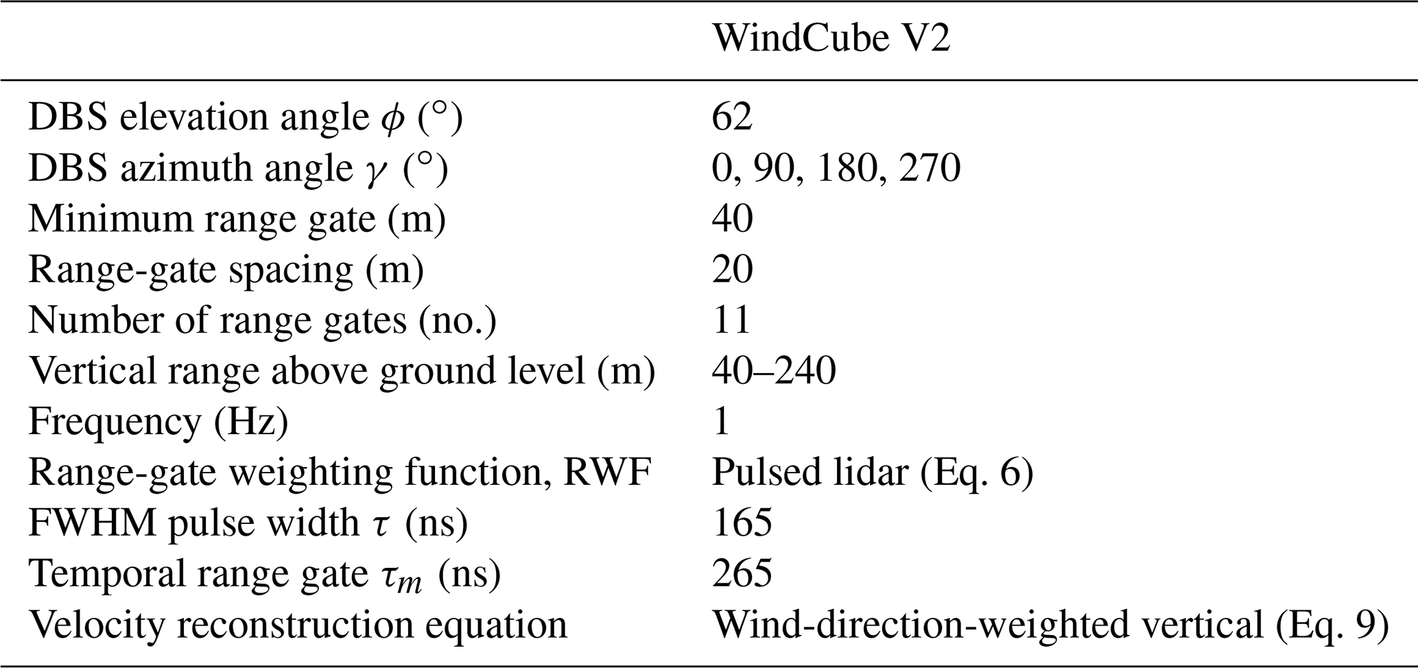
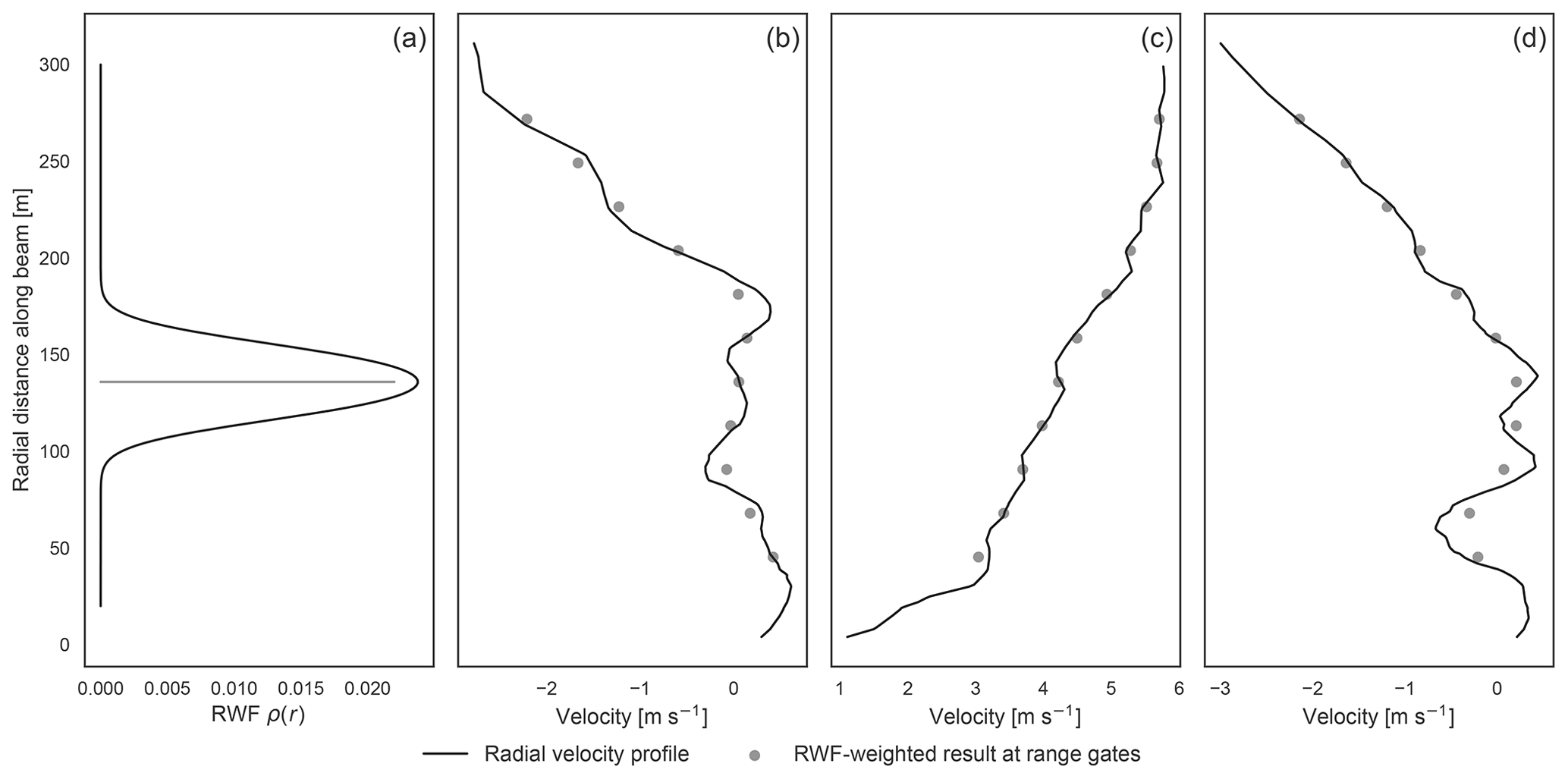
Figure 2 (a) WindCube V2 RWF centered at the 120 m range gate and examples (b, c, d) of unweighted radial velocity profiles, interpolated from instantaneous LES winds, compared to the corresponding weighted result at the range gates.

The RWF for the modeled WindCube V2 (Fig. 2a) results from substituting its range gate and pulse parameters (Table 1) into the general pulsed lidar equation (Eq. 6). The shape of the RWF peaks at the center and tapers symmetrically toward zero to either side. The weights drop to half their peak value about 20 m from the target distance and are non-negligible up to around 40 m. The range-gate parameter in a coherent lidar system must balance the desire for spatial locality and the need for accurate frequencies used in measuring the radial velocity. The more signal points from the traveling pulse used, i.e. the longer the range gate, the more accurate the diagnosis of the frequencies but the longer the averaging volume along the beam. The application of the RWF to the radial velocity profile may be thought of as a smoothing low-pass filter (Fig. 2b, c, d).

To compute the RWF-weighted retrieval from an LES flow field, the wind components are first interpolated to points along the beam and then projected onto the beam direction. The virtual lidar uses a linear barycentric interpolation from a triangulation of the LES grid (i.e. linear interpolation on tetrahedrons using Virtanen et al., 2020). The numerical approximation of the convolution integral of the RWF with the interpolated radial velocities treats the continuous weighted average as a discrete weighted average (Eq. 7). The form is a slightly modified formulation of that used in Lundquist et al. (2015) and Forsting et al. (2017) (see Appendix D).

$$\begin{array}{}\text{(7)}& \begin{array}{rl}{\stackrel{\mathrm{‾}}{v}}_r\left(r_{\mathrm{0}}\right)& =\underset{-\mathrm{\infty }}{\overset{\mathrm{\infty }}{\int }}\mathit{\rho }\left(s\right)v_{\mathrm{r}}(r_{\mathrm{0}}+s)\mathrm{d}s\approx \underset{-R}{\overset{R}{\int }}\mathit{\rho }\left(s\right)v_{\mathrm{r}}(r_{\mathrm{0}}+s)\mathrm{d}s\\ & \approx \sum _k{\displaystyle \frac{h_k\mathit{\rho }\left(s_k\right)}{{\sum }_i{h}_i\mathit{\rho }\left(s_i\right)}}{v}_{\mathrm{r}}(r_{\mathrm{0}}+s_k)\end{array}\end{array}$$

Parameterizing along the beam, the {s_i} nodes are the points where the winds have been interpolated (s_i=0 is at r₀). If the nodes are taken to be midpoints of intervals with corresponding lengths {h_i} that partition the integral range, $[-R,R]$, then the quadrature formulation is a normalized midpoint rule. The normalization ensures the result is a weighted average (avoiding over- or under-estimation due to the numeric weights not summing to unity). The placement of the nodes {s_i} is free to be chosen for convenience or, as recommended by Forsting et al. (2017), to optimize utility of the interpolated points in the convolution so that fewer points need be interpolated. Our current implementation uses equispaced points 1 m apart along the beam (see Appendix D for discussion).

2.1.2 Time-resolved scanning patterns

Based on the type of scan they perform, lidars are categorized as profiling or scanning systems. Profiling lidars are designed to provide a vertical profile of the 3D wind velocity, much as would be reported by a meteorological tower. To reconstruct a 3D wind vector, the instrument needs spanning radial velocity samples from at least three different directions. The scan is completed quickly to limit the intervening evolution of the wind field. Any scanning geometry, such as that described here or other common or complex options as in Clifton et al. (2015), arises from “pointing” the beam and is most naturally and compactly represented as a time series of elevation, ϕ, and azimuthal, γ, angles in spherical coordinates with the beam source at the origin.

For the purposes of this study, we consider the DBS profiling scan used by the WindCube V2, which moves through the four cardinal directions, angled 62^∘ from the horizon, before pointing the beam straight vertically (Fig. 1). The total scan takes approximately 5 s, spending about a second at each of the scan positions (Bodini et al., 2019). The range gates correspond to equispaced heights above the ground. The vertical range of the WindCube V2 is determined by the number and spacing of the range gates, and a typical configuration for the instrument has 11 range gates spaced vertically every 20 m from 40 to 240 m above ground level (Table 1). As the beam rotates through the scan, radial velocities are measured at the center and four points around the circular perimeter of the scanning cone for each given height. At each second in the post-processing stage, the most recent set of radial velocities is used to reconstruct an estimate of the vertical profile of 3D velocities.

The beam accumulation time for the WindCube V2 is about a second, whereas the LES model time steps are on the order of a 10th of a second. The additional averaging due to the longer accumulation time is ignored in the current version of the virtual lidar; it handles the scan by performing the beam sampling on snapshots of the flow field output at 1 s intervals. It is assumed that in the WindCube V2, the temporal average is less significant than the spatial averaging; future versions of the model will account for accumulation times by performing this averaging step explicitly.

2.1.3 Internal processing: 3D velocity reconstruction

In the WindCube V2, the post-processing stage reconstructs the 3D velocity from the radial velocities collected across the scan cycle. Under the assumptions of horizontal homogeneity (i.e. constant winds) over the scan volume and invariance over the scan duration, the radial velocities collected by each of the beams at a given height are all projections of the same 3D velocity vector. Omitting the vertical beam, we solve for the vector components at a given range-gate height (Eq. 8) (Cariou and Boquet, 2010).

$$\begin{array}{}\text{(8)}& {\mathit{u}}_l=\left(\begin{array}{c}\frac{v_{r,E}-v_{r,W}}{\mathrm{2}\cos \mathit{\varphi }}\\ \frac{v_{r,N}-v_{r,S}}{\mathrm{2}\cos \mathit{\varphi }}\\ \frac{v_{r,N}+v_{r,E}+v_{r,S}+v_{r,W}}{\mathrm{4}\sin \mathit{\varphi }}\end{array}\right)\end{array}$$

At a fixed height, $v_{r,E,W,N,S}$ represent the most recently measured radial velocities (${\stackrel{\mathrm{‾}}{v}}_r\left(r_{\mathrm{0}}\right)$) from beams pointed in each of the cardinal directions. The elevation angle of the beams from the horizon is ϕ=62^∘.

Later versions of Leosphere's WindCube instruments use a modified reconstruction (Raghavendra Krishnamurthy​​​​​​​, personal communication, 2020) for the vertical velocity (Eq. 9), which weights the beams in the reconstruction using the estimated wind direction, Θ_l, measured clockwise from due north, as presented in Newman et al. (2016) and Sathe et al. (2011). Re-weighting emphasizes beams along the mean wind direction, exploiting the fact that decorrelation distances along the mean wind direction are typically longer than along the cross-stream direction.

$$\begin{array}{}\text{(9)}& {\mathit{u}}_l=\left(\begin{array}{c}\frac{v_{r,E}-v_{r,W}}{\mathrm{2}\cos \left(\mathit{\varphi }\right)}\\ \frac{v_{r,N}-v_{r,S}}{\mathrm{2}\cos \left(\mathit{\varphi }\right)}\\ \frac{(v_{r,N}+v_{r,S}){\cos }^{\mathrm{2}}\left({\mathrm{\Theta }}_l\right)+(v_{r,E}+v_{r,W}){\sin }^{\mathrm{2}}\left({\mathrm{\Theta }}_l\right)}{\mathrm{2}\sin \left(\mathit{\varphi }\right)}\end{array}\right)\end{array}$$

When the mean wind direction is at a 45^∘ angle to the lidar axes (delineated by the south–north and east–west beam pairs), the weights reduce to the uniform one-fourth in the original reconstruction (Eq. 8). When the mean wind aligns directly with one of the lidar axes, only the two respective beams on that axis are used. We compare the error in both approaches as well as the measurement by the vertically pointing beam (Sect. 3.4).

2.2 Idealized atmospheric boundary layer simulations of varying stability

Realistic atmospheric flow fields are generated using LES configurations of the Advanced Research Weather Research and Forecasting (WRF-ARW) model v4.1 (Skamarock et al., 2019). WRF-ARW is a finite difference numerical model that solves the flux form of the fully compressible, nonhydrostatic Euler equations for high-Reynolds-number flows. The model runs on a staggered, Arakawa-C grid with stretched, terrain-following hydrostatic pressure coordinates in the vertical. The simulations in this study employ a third-order Runge–Kutta time integrator and fifth- and third-order horizontal and vertical advection. All simulations use a non-linear backscatter and anisotropy (NBA2) sub-filter-scale stress model (Mirocha et al., 2010).

Table 2 Parameters for WRF-LES runs used to represent different stability regimes.

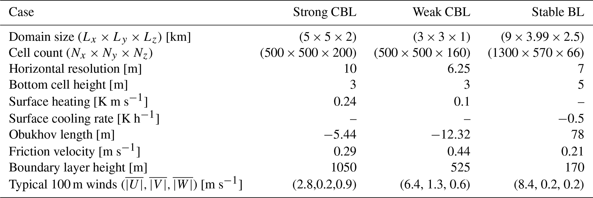
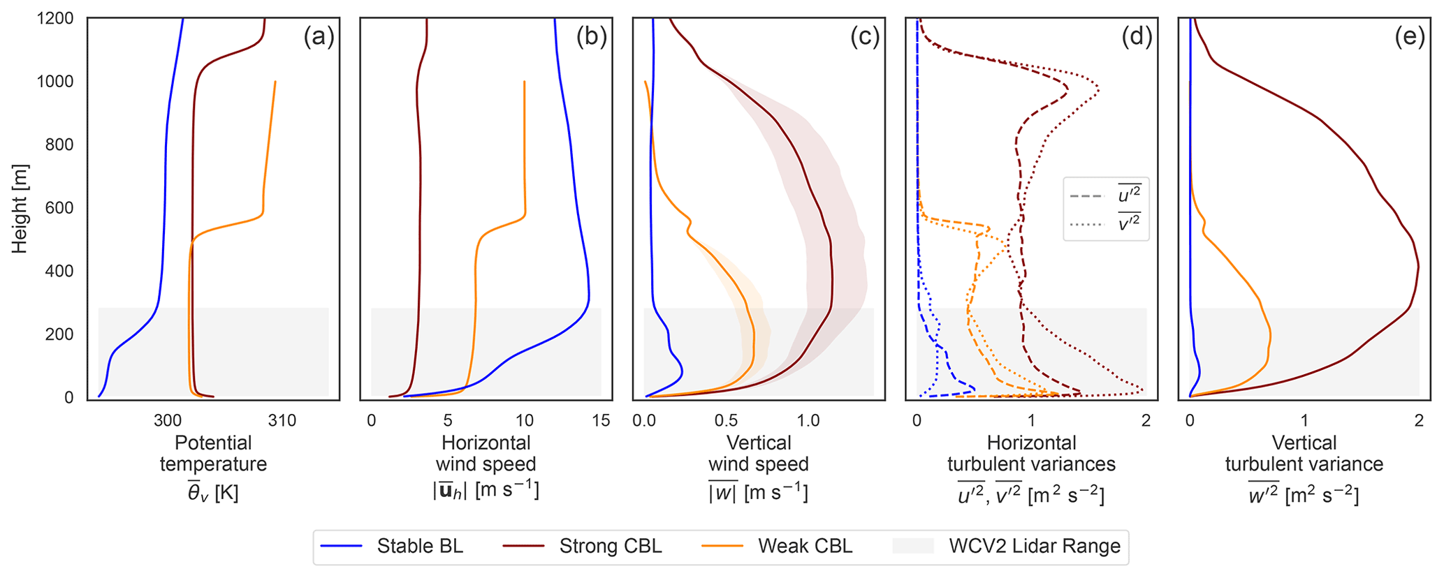
Figure 3 For each of the idealized LES cases, mean profiles of (a) virtual potential temperature, (b) horizontal wind speed, and (c) mean vertical velocity magnitudes with shaded color indicating the span between mean negative and positive values are shown. The turbulent velocity variances, $\stackrel{\mathrm{‾}}{{u^{\prime }}^{\mathrm{2}}}$ (dashed) and $\stackrel{\mathrm{‾}}{{v^{\prime }}^{\mathrm{2}}}$ (dotted), are shown in (d) with $\stackrel{\mathrm{‾}}{{w^{\prime }}^{\mathrm{2}}}$ in panel (e). The grey region demarcates the WindCube V2 vertical range including the region of influence for the range-gate weighting.

To establish a baseline reference for lidar operation in ideal conditions, all simulations in this study use uniform flat, grassy terrain (roughness length z₀=0.1 m); periodic boundary conditions; and temporally and spatially invariant forcing. The idealized scenarios isolate fundamental characteristics of the atmospheric flows, removing potential influence from additional complexities and inhomogeneities, e.g. mesoscale forcing, varied terrain and land cover, and the diurnal cycle or nearby obstructions like wind turbines. None of the simulations in this study incorporate models for moisture, clouds, radiation, microphysics, or land surface. The simulations are distinguished by varying stability: two convective cases and one stable stratification case, detailed in Table 2 and Fig. 3. For each of the simulations, we use 10 min of simulated time after spin-up has been achieved, output at 1 s intervals.

For the convective boundary layers (CBLs), we use data from precursory simulations in Rybchuk et al. (2021), which emulate observed conditions during the Project Prairie Grass campaign (Barad, 1958). Following the labeling therein, we designate the cases as the “strong” and “weak” convective boundary layers. Although both are considered strongly convective by their Obukhov length classification (Muñoz-Esparza et al., 2012) and are largely dominated by cell structures (Salesky et al., 2017), the cases differ meaningfully in the relative strength of the surface heating and geostrophic winds. The strong CBL case features stronger heating and slower winds than the weak CBL.

The stable-boundary-layer simulation closely follows the configuration of Sanchez Gomez et al. (2021). The surface condition for the stable case is driven with a cooling rate, rather than a negative heat flux (Basu et al., 2007). Spinning up a stable case to relatively steady turbulence statistics can also be computationally expensive; a set of two one-way nested domains is used to reduce the computational demand. The parent domain has periodic boundary conditions and a horizontal resolution of 70 m. It evolves for about 13.5 h before the inner domain is started and simulated over the final 45 min. To reduce the fetch required to spin up fine turbulence in the nested interior grid, we employ the cell-perturbation method from Muñoz-Esparza et al. (2014). The first 30 min of data from the fine-scale domain are discarded, and only an interior region excluding fetch and edge effects is used for the virtual lidar sampling.

Mean profiles, computed with data from the valid regions of the LES cases, are characteristic of the respective stability regimes (Fig. 3). Well-developed mixed layers, with consistent virtual potential temperature and wind speeds, account for the majority of the lidar observation range in the convective boundary layers. The bottom two reported range gates, however, incorporate values from the surface layer due to range-gate weighting. The weaker convective case has significantly stronger winds, and the surface heating only supports a boundary layer about half as high as in the strong CBL case. The entrainment zone is out of lidar range in both cases. Vertical velocity magnitudes reach maximum values in the middle of the convective boundary layers, with a notable gap between the mean negative and positive values reflecting strong upward plumes and weaker, broader downdrafts. In the stable case, the boundary layer falls entirely within the lidar range. The distinctive temperature stratification is paired with strong winds that reach a maximum in a jet not far above the top of the boundary layer. Vertical velocities are typically small and balanced and become negligible aloft.

2.2.1 Configuration of virtual WindCube V2 ensemble

A virtual WindCube V2 is created in the lidar model as described in Sect. 2.1 and summarized in Table 1. To maximize realizations of the instrument sampling from each of the LES flows, a grid of 45 instances of the virtual WindCube V2 is placed in each domain. The locations are spaced such that their scanning volumes do not overlap. Each lidar scan coincides uniquely with surrounding flow structures, comprising a statistical sample of how the instrument might interact with the distinctive atmospheric variability of each regime.

The mean background states of the LES cases are spatially and temporally consistent across the domain, including the direction of the prevailing winds. To account for potential differences due to the relative orientation of the lidar axes in the flow, the ensemble of virtual lidar instruments is re-oriented at three additional offset angles (15, 30, 45^∘) and allowed to sample the LES fields again. The negligible sensitivity of the error to the relative orientation is discussed in Sect. 3.2.

Determining the error in the lidar observation depends on defining a reference truth. Profiling lidars are often thought of as replacing meteorological towers, returning a vertical profile of 3D velocities similar to a tower fitted with instruments, but what value the lidar should actually be thought of as measuring is not so straightforward. The samples used to estimate the wind components lack the precise locality of tower instruments; the beams collecting line-of-sight data span an increasingly large area with height, each incorporating a vertical extent via the RWF. These factors suggest that a volume average might be a more appropriate reference truth (as suggested in Courtney et al., 2008). The lidar reflects pieces of both representations: it has the spatial spread of the volume average but depends on only a handful of points on the edge of the volume that impart higher variability similar to a pointwise profile.

Along with a “pointwise” tower-style truth profile of interpolated velocities above the instrument, we determined a volume-averaged profile for each lidar. The volume average is computed as the mean of all LES points that fall inside cylinders tracing the lidar scan radius (Fig. 1). Centered at each range gate, the cylinders are defined to have a radius equal to that of the scan cone and height corresponding to the vertical projection of the RWF range resolution. For the WindCube V2, the range resolution is the FWHM of the RWF so that the cylinders are 40sin (ϕ)≈ 35.3 m tall. At the lowest levels with the smallest volumes, a minimum of around 80 LES points are used, which increases to several hundred points in the top cylinders.

2.3 Random-variable model of error

Alongside the virtual model of the lidar, we develop an analytic model of the measurement error which serves to help explain the mechanisms at work and interpret the results of the virtual measurements. The following analysis systematically addresses how turbulent variations induce error in the wind reconstruction and how that error propagates into derived quantities. Much of the analysis presented in this section is quite general and applies to any DBS reconstruction of the form of Eq. (8) and in any flow condition. The approach can be extended to different scan types as well in decomposing their error.

Two elements directly introduce error into the observation model: the application of the RWF in the radial velocity measurement and the assumption of horizontal uniformity in the reconstruction. Using a random variable model, we identify the contributions of the RWF and horizontal velocity variations to the error in the wind component reconstructions. Duration of the scan cycle and time staggering of the beams are not explicitly addressed in the error model, though they are included in the implementation of the virtual instrument.

Quantities derived from the estimated wind components can take on their own non-trivial error behavior. Natural derived quantities that are often computed from lidar data include horizontal wind speed and direction and time-averaged winds. We characterize the error in wind speed and direction in terms of the u and v error distributions and trace the expected effect of time averaging on the error distributions.

2.3.1 Wind component reconstruction

We start by deriving the form of the error in the reconstructed velocity components. The formulation allows the contribution to the error due to the turbulent variations to be explicitly delineated and tracked. For a fixed height, let $\mathit{U}=(U,V,W{)}^T$ be the mean velocity across the scan volume, i.e. the volume-averaged truth, and assume that it is constant through the 5 s scan duration. Different notions of the volume average could be used here, e.g. the two- or four-point average over the beam locations, but the disk seems the most useful average representation to measure. Each angled beam samples a perturbed velocity, ${\mathit{u}}_{E,W,N,S}\left(t\right)=\mathit{U}+{\mathit{u}}_{E,W,N,S}^{\prime \prime }\left(t\right)$, where the subscript denotes the cardinal direction of the beam azimuthal direction. The measurement of the projection of the point velocity is subject to an additional perturbation, $r_{E,W,N,S}$, due to the RWF. Then, the radial velocity measured by the beam pointed east, for example, is given in Eq. (10).

$$\begin{array}{}\text{(10)}& {\displaystyle }{v}_{r,E}=\cos \left(\mathit{\varphi }\right)(U+u_E^{\prime \prime })+\sin \left(\mathit{\varphi }\right)(W+w_E^{\prime \prime })+r_E\end{array}$$

Carrying the forms through the reconstruction (Eq. 8), the error in the wind components is given by the difference with the volume-averaged value, U. (This analysis is similar to that of Newman et al. (2016), which extends the derivation to turbulent variances.) The vertical velocity error form depends on whether the wind direction weighting is used; we limit our error model analysis to the equally weighted version (Eq. 11).

$$\begin{array}{}\text{(11)}& \begin{array}{rl}& {\mathit{u}}_{\mathrm{err}}={\mathit{u}}_l-\mathit{U}=\\ & \left(\begin{array}{c}\frac{\mathrm{1}}{\mathrm{2}}\left[(u_E^{\prime \prime }+u_W^{\prime \prime })+\tan \left(\mathit{\varphi }\right)(w_E^{\prime \prime }-w_W^{\prime \prime })\right.\\ \left.+\sec \left(\mathit{\varphi }\right)(r_E-r_W)\right]\\ \frac{\mathrm{1}}{\mathrm{2}}\left[(v_N^{\prime \prime }+v_S^{\prime \prime })+\tan \left(\mathit{\varphi }\right)(w_N^{\prime \prime }-w_S^{\prime \prime })\right.\\ \left.+\sec \left(\mathit{\varphi }\right)(r_N-r_S)\right]\\ \frac{\mathrm{1}}{\mathrm{4}}\left[(w_N^{\prime \prime }+w_E^{\prime \prime }+w_S^{\prime \prime }+w_W^{\prime \prime })\right.\\ +\cot \left(\mathit{\varphi }\right)(u_E^{\prime \prime }-u_W^{\prime \prime }+v_N^{\prime \prime }-v_S^{\prime \prime })\\ \left.+\csc \left(\mathit{\varphi }\right)(r_N+r_E+r_S+r_W)\right]\end{array}\right)\end{array}\end{array}$$

In a perfectly horizontally uniform wind field, the velocity perturbation values all individually vanish (i.e. not due to cancelations). However, even in that perfectly horizontally uniform case, a non-linear vertical profile can still induce non-zero error through the RWF.

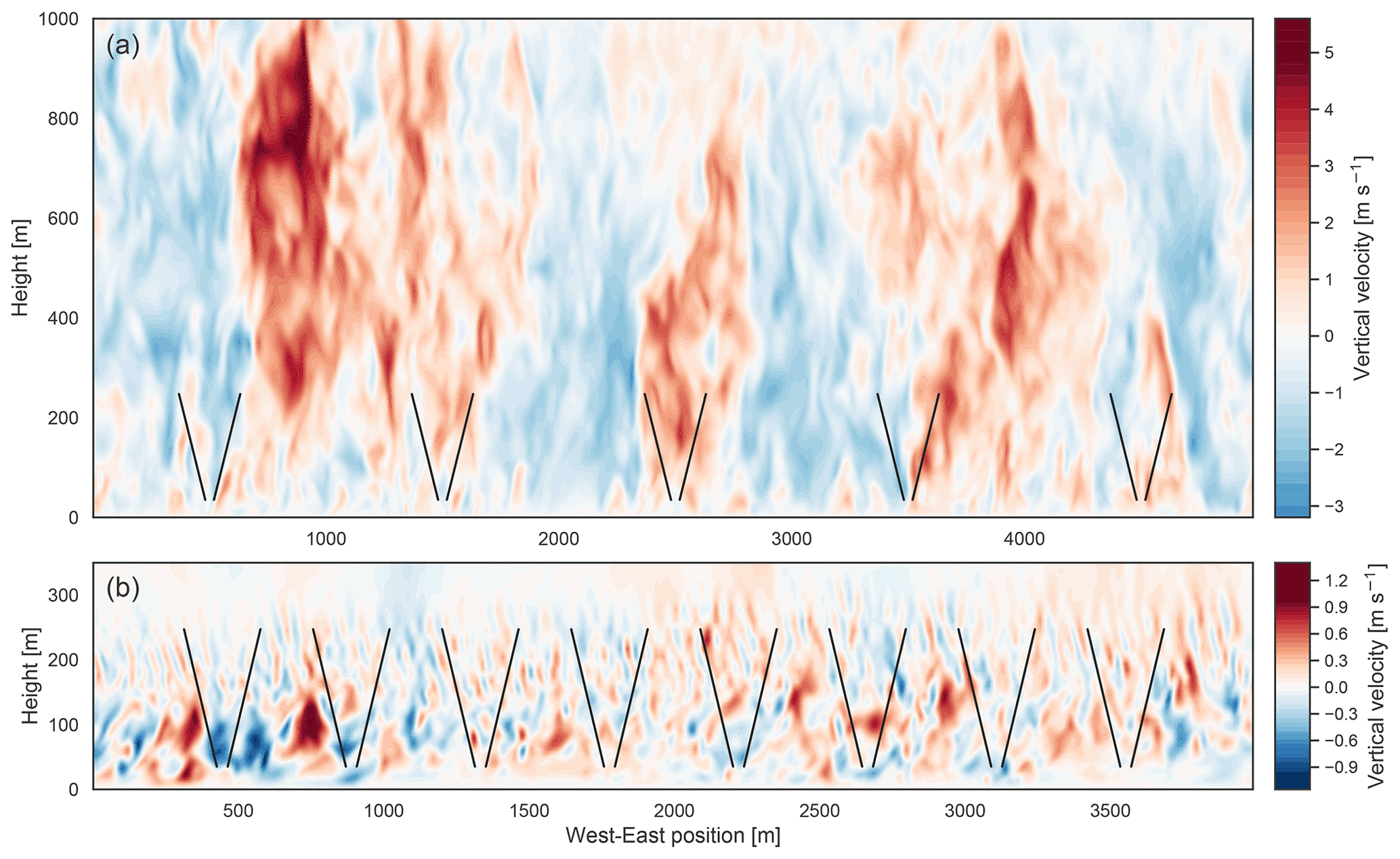
Figure 4 Instantaneous slice of vertical velocity across the west–east plane in (a) the strong CBL and (b) the stable BL. The WindCube V2 scan geometry is shown for reference by the beams in black.

In the presence of turbulence in the flow, the velocity over the scan volume is no longer uniform, and the beams sample perturbed variations, violating the assumption underlying the exact reconstruction. The perturbation values may be regarded as random variables with distributions resulting from the character of the atmospheric variations and the lidar scan geometry (Fig. 4). Under this model, spatial trends in the background flow would be expressed in shifted perturbation mean values at the respective beam locations. The error formulation defines how the turbulent variations in separate wind components and RWF effects combine to produce the total error.

As functions of the random perturbations, the wind component errors are themselves random variables. The mean, μ, and variance, σ², of the error distributions can be expressed in terms of the perturbation distributions through algebra of random variables (Zwillinger and Kokoska, 2000). The mean of the error distribution describes offsets, or biases, in the error; it represents how quantities are consistently over- or under-estimated. The variance of the error describes the spread in the error values; it reflects the magnitude of errors on top of any systematic mean bias.

The mean operator is linear and directly decomposes the overall error mean into constituent parts for the horizontal (Eq. 12) and vertical (Eq. 13) wind components.

$$\begin{array}{}\text{(12)}& \begin{array}{rl}\mathit{\mu }\left(u_{\mathrm{err}}\right)& ={\displaystyle \frac{\mathrm{1}}{\mathrm{2}}}\left[\mathit{\mu }\right(u_E^{\prime \prime })+\mathit{\mu }(u_W^{\prime \prime }\left)\right]+{\displaystyle \frac{\tan \left(\mathit{\varphi }\right)}{\mathrm{2}}}\left[\mathit{\mu }\left(w_E^{\prime \prime }\right)\right.\\ & \left.-\mathit{\mu }\left(w_W^{\prime \prime }\right)\right]+{\displaystyle \frac{\sec \left(\mathit{\varphi }\right)}{\mathrm{2}}}\left[\mathit{\mu }\right(r_E)-\mathit{\mu }(r_W\left)\right]\end{array}\end{array}$$

$$\begin{array}{}\text{(13)}& \begin{array}{rl}\mathit{\mu }\left(w_{\mathrm{err}}\right)& ={\displaystyle \frac{\mathrm{1}}{\mathrm{2}}}\left[\mathit{\mu }\right(w_E^{\prime \prime })+\mathit{\mu }(w_W^{\prime \prime })+\mathit{\mu }(w_N^{\prime \prime })+\mathit{\mu }(w_S^{\prime \prime }\left)\right]\\ & +{\displaystyle \frac{\cot \left(\mathit{\varphi }\right)}{\mathrm{2}}}\left[\mathit{\mu }\right(u_E^{\prime \prime })-\mathit{\mu }(u_W^{\prime \prime })+\mathit{\mu }(u_N^{\prime \prime })-\mathit{\mu }(u_S^{\prime \prime }\left)\right]\\ & +{\displaystyle \frac{\csc \left(\mathit{\varphi }\right)}{\mathrm{2}}}\left[\mathit{\mu }\right(r_E)+\mathit{\mu }(r_W)+\mathit{\mu }(r_N)+\mathit{\mu }(r_S\left)\right]\end{array}\end{array}$$

The variance (σ²) can also be decomposed into a linear combination of constituent terms but introduces covariance terms (Eqs. 14 and 15). The variance is preferred here to the standard deviation (σ) so that the contributions are additive (i.e. no square root). We do not explicitly expand the covariance terms, which quantify correlations between the perturbations.

$$\begin{array}{}\text{(14)}& {\displaystyle }\begin{array}{rl}{\mathit{\sigma }}^{\mathrm{2}}\left(u_{\mathrm{err}}\right)& ={\displaystyle \frac{\mathrm{1}}{\mathrm{4}}}\left[{\mathit{\sigma }}^{\mathrm{2}}\right(u_E^{\prime \prime })+{\mathit{\sigma }}^{\mathrm{2}}(u_W^{\prime \prime }\left)\right]+{\displaystyle \frac{{\tan }^{\mathrm{2}}\left(\mathit{\varphi }\right)}{\mathrm{4}}}\left[{\mathit{\sigma }}^{\mathrm{2}}\left(w_E^{\prime \prime }\right)\right.\\ & \left.+{\mathit{\sigma }}^{\mathrm{2}}\left(w_W^{\prime \prime }\right)\right]+{\displaystyle \frac{{\sec }^{\mathrm{2}}\left(\mathit{\varphi }\right)}{\mathrm{4}}}\left[{\mathit{\sigma }}^{\mathrm{2}}\right(r_E)+{\mathit{\sigma }}^{\mathrm{2}}(r_W\left)\right]\\ & +\text{covariance terms}\end{array}\text{(15)}& {\displaystyle }\begin{array}{rl}& {\mathit{\sigma }}^{\mathrm{2}}\left(w_{\mathrm{err}}\right)={\displaystyle \frac{\mathrm{1}}{\mathrm{4}}}\left[{\mathit{\sigma }}^{\mathrm{2}}\right(w_E^{\prime \prime })+\mathit{\mu }(w_W^{\prime \prime })+{\mathit{\sigma }}^{\mathrm{2}}(w_N^{\prime \prime })+{\mathit{\sigma }}^{\mathrm{2}}(w_S^{\prime \prime }\left)\right]\\ & +{\displaystyle \frac{{\cot }^{\mathrm{2}}\left(\mathit{\varphi }\right)}{\mathrm{4}}}\left[{\mathit{\sigma }}^{\mathrm{2}}\right(u_E^{\prime \prime })+{\mathit{\sigma }}^{\mathrm{2}}(u_W^{\prime \prime })+{\mathit{\sigma }}^{\mathrm{2}}(u_N^{\prime \prime })+{\mathit{\sigma }}^{\mathrm{2}}(u_S^{\prime \prime }\left)\right]\\ & +{\displaystyle \frac{{\csc }^{\mathrm{2}}\left(\mathit{\varphi }\right)}{\mathrm{4}}}\left[{\mathit{\sigma }}^{\mathrm{2}}\right(r_E)+{\mathit{\sigma }}^{\mathrm{2}}(r_W)+{\mathit{\sigma }}^{\mathrm{2}}(r_N)+{\mathit{\sigma }}^{\mathrm{2}}(r_S\left)\right]\\ & +\text{covariance terms}\end{array}\end{array}$$

The relative weighting of the perturbations is controlled by the scan cone elevation angle from the horizon, ϕ (Fig. 1), and describes the result of the relative projection of the perturbations on the beam. For the WindCube V2 cone angle, tan ϕ≈1.88, so that the vertical velocity perturbations are weighted almost twice as heavily as the horizontal velocity perturbations. The radial velocity perturbations are similarly heavily weighted, with sec ϕ≈2.1. The asymmetric weighting is further exacerbated in the variance, which uses the squares of these values.

Along with the relative weights, the elevation angle controls the spatial separation of the beams, thus implicitly influencing the distributions of the perturbations themselves. The beam separation can be of particular importance in the presence of background spatial variation in the flow in which larger separation can induce a greater mean error, as explored in terms of linear variations in vertical velocity in Bingöl et al. (2009). Teschke and Lehmann (2017) derived a shallow elevation angle (ϕ≈35.26^∘) as minimizing error in the reconstruction in the presence of noisy radial velocity measurements in locally homogeneous conditions. The magnitude of the radial velocity variances is not constant, instead varying with the elevation angle and the resulting projection of the turbulent fluctuations onto the beam.

More off-vertical beams may be used with a linear least-squares reconstruction process (Newsom et al., 2015), of which the DBS scan presented in this study is a special case. The beams are usually preferred to be symmetrically spaced to cancel potential systematic biases in the u and v reconstructions (Sathe et al., 2015; Teschke and Lehmann, 2017).

The virtual lidar model uses the LES to indirectly predict the perturbation distributions and the complex ways in which the perturbations can be inter-related with each other and with respect to the volume averages. Random variable theory can then be used to describe the propagation of uncertainty into the error from the attributes of the perturbation distributions.

2.3.2 Effects of range-gate weighting

The size of discrepancies in the radial velocity measurement due to weighting by the RWF may be analytically bound. The bound serves to illuminate the conditions under which the perturbations from the point value can become large.

Assume any RWF, ρ(s), is a non-negative, even function that monotonically decays as $s\to \pm \mathrm{\infty }$ and satisfies ${\int }_{-\mathrm{\infty }}^{\mathrm{\infty }}\mathit{\rho }\left(s\right)=\mathrm{1}$. Let v_r(r) be the radial velocity profile along the beam and R>0 a threshold distance from the target, r₀. Then under the RWF model, the size of the discrepancy between the range-gate-weighted measurement, ${\stackrel{\mathrm{‾}}{v}}_r\left(r_{\mathrm{0}}\right)$, and the actual pointwise radial velocity, v_r(r₀), is constrained in Eq. (16) (derivation in Appendix C).

$$\begin{array}{}\text{(16)}& \begin{array}{rl}& \left|{\stackrel{\mathrm{‾}}{v}}_r\left(r_{\mathrm{0}}\right)-v_{\mathrm{r}}\left(r_{\mathrm{0}}\right)\right|\le \\ & \left[\mathrm{1}-\underset{\left|s\right|\le R}{\int }\mathit{\rho }\left(s\right)\mathrm{d}s\right]\left(\underset{s>\left|R\right|}{max}\left|v_{\mathrm{r}}\right(r_{\mathrm{0}}+s\left)\right|+\left|v_{\mathrm{r}}\right(r_{\mathrm{0}}\left)\right|\right)\\ & +\left[{\displaystyle \frac{\mathrm{1}}{\mathrm{2}}}\underset{\left|s\right|\le R}{\int }\mathit{\rho }\left(s\right)s^{\mathrm{2}}\mathrm{d}s\right]\left|v_{\mathrm{r}}^{\prime \prime }\right(r_{\mathrm{0}}+{\mathit{\xi }}_{*}\left)\right|\end{array}\end{array}$$

The bounding terms can be forced to be small by selecting R to manipulate the coefficients. The magnitude of the radial velocities in the atmosphere can practically be expected to be finitely bound. Taking R to be large drives the integral of ρ(s) to 1 and thus the first term to zero. The second term does the opposite: the coefficient grows rapidly with R and is small for small R. The tension between the requirements picks out the conditions that allow for potentially large deviations in the weighted measurement from the true point value.

Radial velocity profiles with constant gradient do not incur error in the RWF application; symmetry leads the linear contributions to cancel. Indeed, visual inspection confirms this behavior in regions of constant gradient about r₀, which incur only small discrepancies (Fig. 2b, c, d). The competition between the remaining bounding terms (Eq. 16) places requirements on the radial velocity behavior itself; in the absence of large curvature in the radial velocity profile ($\left|v_{\mathrm{r}}^{\prime \prime }\right|$ small), the error can be expected to be negligible. The largest misrepresentations appear in areas with sharp bends in the radial velocity profile (Fig. 2).

2.3.3 Horizontal uniformity violations

Variations in the velocity across the scan volume are directly represented in the error model by the velocity perturbations in the wind component errors (Eq. 11). Horizontal variations may also be reflected in the radial velocity along the beam and are assumed to be encapsulated in the treatment of the RWF. The perturbations in the velocity around the scan radius occur due to variations over a larger spatial scale than those along a single beam, potentially permitting larger turbulent structures with larger variations.

To describe the error due to the perturbation terms, we consider what they represent and how they relate to the turbulence in the flow. In the lidar model, the velocity perturbations (${\mathbf{u}}_{E,W,N,S}^{\prime \prime }$) are taken with respect to the average over the scan volume; they are a kind of turbulent fluctuation under the high-pass filter based on the scale of the scan volume (about 42 m across at the bottom range gate and 255 m at the top), filtering out turbulence at the larger scales. The variance of the perturbations, ${\mathit{\sigma }}^{\mathrm{2}}\left(u_{E,W,N,S}^{\prime \prime }\right)$, which determines their magnitude, is a filtered fraction of the full-turbulence velocity variance, $\stackrel{\mathrm{‾}}{{u^{\prime }}^{\mathrm{2}}}$. As the size of the scan volume increases, the volume average approaches an ensemble mean so that the perturbations become Reynolds fluctuations, u^′. The variance expected in the lidar perturbations is determined by the proportion of turbulent variances in each direction above the filter scale, with the full turbulent variance constituting a cap on the total possible variance.

It is tempting, with usual conventions about turbulent perturbations, to assume that the lidar velocity perturbations will have zero mean and identical distributions at each of the beam locations. Under these assumptions, the mean error due to the horizontal homogeneity violations would be zero. However, the volume average over the disk is neither the direct mean of the beam velocities nor the turbulent ensemble mean. The velocity perturbations can produce a non-zero mean because of consistently occurring spatial patterns in how the velocities vary at the edges of the scan volume with respect to the average velocity over that volume. The spatial structures at play in the LES cases with respect to the lidar scan volume can be seen in the cross sections in Fig. 4. If the turbulent structures are small enough and the scan volume large enough, then the volume average approaches a turbulent ensemble mean so that the beams sample independent turbulent fluctuations. Under such conditions, the assumption of zero mean and identically distributed perturbations at each beam is appropriate. When coherent turbulent structures occur that fill the scan volume, however, the volume average no longer represents a turbulent ensemble mean. Without dissecting the mechanics more closely, we simply note that large coherent structures, like turbulent plumes characteristic of the convective boundary layer, can induce repeated, non-symmetric patterns in the relative perturbations of the beams, leading to non-zero means.

2.3.4 Secondary effect on derived quantities: wind speed and direction

The horizontal wind vector is commonly represented not by its components but by the wind speed, $\left|{\mathit{U}}_h\right|$, and direction, Θ. The WindCube V2 internally computes and reports these quantities, derived from the reconstructed u and v components (Eq. 17).

$$\begin{array}{}\text{(17)}& {\displaystyle }\left|{\mathit{u}}_{h,l}\right|=\sqrt{u_l^{\mathrm{2}}+v_l^{\mathrm{2}}},{\mathrm{\Theta }}_l=\arctan \mathrm{2}(-u_l,-v_l)\end{array}$$

The wind direction, placed in the appropriate quadrant, is compactly represented by the two-argument inverse tangent (the sign and order of the arguments follow meteorological conventions with the angle measuring the wind source clockwise from north). Wind direction error is bound in the interval (−180, 180^∘), where positive values indicate the lidar reading an angle clockwise from truth and negative values an angle counterclockwise from truth (Fig. 5).

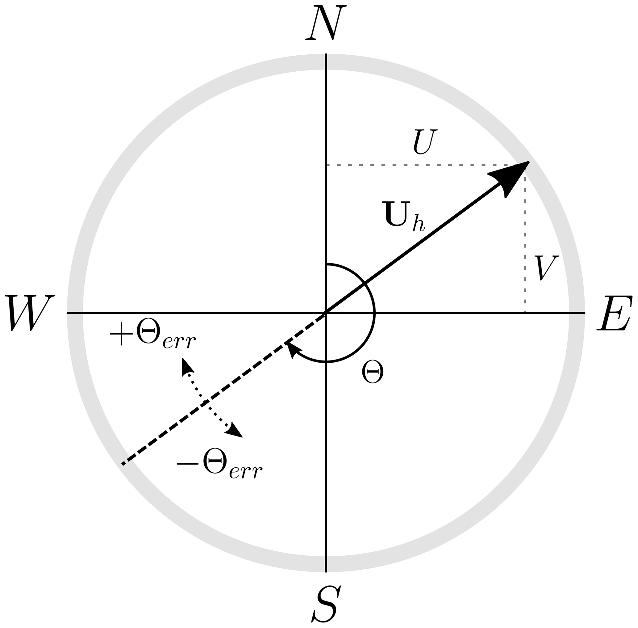
Figure 5 Conventions used for the horizontal wind vector direction and signs of the wind direction error.

The derived values do not inherit the error from the wind component errors directly; rather the quantities should be thought of as functions of the u and v errors treated earlier, taking on their own distinct, related error distribution behavior. As non-linear functions of u and v, the errors in the wind speed and direction do not drop out directly.

We may expand the lidar-sensed horizontal wind speed (Eq. 17) about the volume-averaged wind speed, using ${\mathbf{u}}_{h,l}={\mathbf{U}}_h+{\mathbf{u}}_{h,\mathrm{err}}$. (The error compared to a pointwise reference is better served by expanding both about an average reference.) We assume the errors in u and v to be small and take a second-order Taylor-series expansion of the square root. Then we obtain Eq. (18) (by mathematical analog to the Reynolds decomposition, echoing Rosenbusch et al., 2021).

$$\begin{array}{}\text{(18)}& \begin{array}{rl}|{\mathit{U}}_h{|}_{\mathrm{err}}& =\left|{\mathit{u}}_{h,l}\right|-\left|{\mathit{U}}_h\right|\approx {\displaystyle \frac{U}{\left|{\mathit{U}}_h\right|}}{u}_{\mathrm{err}}+{\displaystyle \frac{V}{\left|{\mathit{U}}_h\right|}}{v}_{\mathrm{err}}\\ & +{\displaystyle \frac{(\frac{U}{\left|{\mathbf{U}}_h\right|}{v}_{\mathrm{err}}-\frac{V}{\left|{\mathbf{U}}_h\right|}{u}_{\mathrm{err}}{)}^{\mathrm{2}}}{\mathrm{2}\left|{\mathbf{U}}_h\right|}}={\displaystyle \frac{{\mathit{U}}_h}{\left|{\mathit{U}}_h\right|}}\cdot {\mathit{u}}_{h,\mathrm{err}}\\ & +{\displaystyle \frac{{\left|{\left(\frac{U}{\left|{\mathbf{U}}_h\right|},\frac{V}{\left|{\mathbf{U}}_h\right|},\mathrm{0}\right)}^T\times {\left(u_{\mathrm{err}},v_{\mathrm{err}},\mathrm{0}\right)}^T\right|}^{\mathrm{2}}}{\mathrm{2}\left|{\mathit{U}}_h\right|}}\end{array}\end{array}$$

We can explicitly find a theoretical mean of the wind speed error and simplify by assuming the u and v error random variables have a mean of zero (Appendix B) and are uncorrelated.

$$\begin{array}{}\text{(19)}& {\displaystyle }\mathit{\mu }\left(\right|{\mathit{U}}_h{|}_{\mathrm{err}})\approx {\displaystyle \frac{{\cos }^{\mathrm{2}}\mathrm{\Theta }{\mathit{\sigma }}^{\mathrm{2}}\left(u_{\mathrm{err}}\right)+{\sin }^{\mathrm{2}}\mathrm{\Theta }{\mathit{\sigma }}^{\mathrm{2}}\left(v_{\mathrm{err}}\right)}{\mathrm{2}\left|{\mathit{U}}_h\right|}}\end{array}$$

The persisting strictly positive term implies we should expect a systematic positive bias in the wind speed error, i.e. that the wind speed will be over-estimated more than under-estimated. Note that this does not mean the total error (Eq. 18) is always positive – the weighted component errors can cause it to be negative – but that on average the reported wind speed will be greater than that of the actual volume-averaged horizontal wind. The expected magnitude of the bias is proportional to the variance of the error in the u and v measurements and inversely proportional to the volume-averaged wind speed.

Without explicitly computing the variance, we can estimate the magnitude of the wind speed error. Based on the leading order terms, the error should generally be on the order of the individual component errors (i.e. their standard deviation), though the bias term has the potential to become more prominent in adverse conditions (large u and v errors, slow winds).

Now consider the wind direction error. To simplify the analysis, we set aside the quadrant correction and consider just the traditional inverse tangent function to find the angle in [−90, 90^∘]. Then the wind direction error, in radians, is the difference.

$$\begin{array}{}\text{(20)}& {\displaystyle }{\mathrm{\Theta }}_{\mathrm{err}}={\mathrm{\Theta }}_l-\mathrm{\Theta }=\arctan \left({\displaystyle \frac{u_l}{v_l}}\right)-\arctan \left({\displaystyle \frac{U}{V}}\right)\end{array}$$

As with the wind speed, the mean value does not directly cancel. Applying the difference identity for arctan and simplifying,

$$\begin{array}{}\text{(21)}& {\displaystyle }{\mathrm{\Theta }}_{\mathrm{err}}=\arctan \left({\displaystyle \frac{V{u}_{\mathrm{err}}-U{v}_{\mathrm{err}}}{|{\mathit{U}}_h{|}^{\mathrm{2}}+V{v}_{\mathrm{err}}+U{u}_{\mathrm{err}}}}\right).\end{array}$$

The form in Eq. (21) may be turned into a looser bound that is simpler to interpret. The derivative of arctan is continuous and bound above by 1 so that we may bound $\left|\arctan \right(x\left)\right|\le \left|x\right|$. For the error,

$$\begin{array}{}\text{(22)}& {\displaystyle }\left|{\mathrm{\Theta }}_{\mathrm{err}}\right|\le \left|{\displaystyle \frac{\frac{V}{\left|{\mathit{U}}_h\right|}{u}_{\mathrm{err}}-\frac{U}{\left|{\mathit{U}}_h\right|}{v}_{\mathrm{err}}}{\left|{\mathit{U}}_h\right|+v_{\mathrm{err}}+u_{\mathrm{err}}}}\right|.\end{array}$$

The bound is tighter the smaller the error, and the sign of the bounding expression should match that of the error, creating an “envelope” for the error. From the error approximation, if we again assume the reconstruction of u and v to have zero mean error and similar variances, then the wind direction mean error should also be zero (Appendix  B). Without explicitly computing the variance, we estimate the bound on the wind direction magnitude to be (in radians) roughly proportional to the standard deviation of the u and v errors over the volume-averaged wind speed.

2.3.5 Reducing error through time averaging

Time averaging is a tool used to reduce the variation in the error in the raw high-frequency measurements made by the lidar, leaving a more reliable mean measurement. Under conditions in which the background flow continues to evolve in time, the utility of time averaging must be weighed against the length of the interval during which quasi-stationary conditions exist and the sacrificed resolution of shorter timescale dynamics. Making an informed assessment of an appropriate time window length rests on quantifying the expectation of the improvement of the measurement accuracy.

The lidar error varies along with the “random” turbulence in the flow, which we have reflected by describing the error as a random variable that is drawn from a distribution dependent on the character of the turbulence and the lidar scan geometry. Here, we consider how time averaging acts on the error distribution of the raw 1 Hz measurements.

First, we consider a time average (arithmetic mean) performed over the wind components (which is mathematically equivalent to averaging over the beam radial velocities when the reconstruction is linear as in Eq. 8). The following derivations are given in terms of u, but hold identically for all of the wind components ($u,v,w$). Let T be the length of time window and suppose the instrument samples at a constant interval of τ_s (every second for the WindCube V2). Then there are $T_s=\lfloor T/{\mathit{\tau }}_s\rfloor$ samples in the discrete time average over the window. Expanding the lidar estimate of the time-averaged truth, ${\stackrel{\mathrm{‾}}{U}}^T$, the error in the time-averaged measurement emerges by linearity to be the arithmetic mean of the sample errors (Eq. 23).

$$\begin{array}{}\text{(23)}& {\displaystyle }{\stackrel{\mathrm{‾}}{u}}_{\mathrm{err}}^T={\displaystyle \frac{\mathrm{1}}{T_s}}\sum _{i=\mathrm{1}}^{T_s}{u}_{\mathrm{err}}\left(t_i\right)\end{array}$$

That is, the error in the time-averaged measurement can be expressed as the sum of (scaled) random variables drawn from the distribution of the constituent 1 Hz errors. Again using linearity, the mean of the time-averaged error distribution, ${\stackrel{\mathrm{‾}}{u}}_{\mathrm{err}}^T$, is equal to the mean of the original sample errors, $\mathit{\mu }\left({\stackrel{\mathrm{‾}}{u}}_{\mathrm{err}}^T\right)=\mathit{\mu }\left(u_{\mathrm{err}}\right)$; i.e. time averaging does not change the mean ensemble error of the wind components.

The primary effect of the time average on the velocity components is to reduce the width of the error distribution, i.e. the typical magnitude of the errors. The variance of the arithmetic mean of independent, identically distributed random variables is well-known (Zwillinger and Kokoska, 2000); given the variance of the original un-averaged random variable, σ²(u_err), the variance of the mean over N samples is $\frac{\mathrm{1}}{N}{\mathit{\sigma }}^{\mathrm{2}}\left(u_{\mathrm{err}}\right)$. In a time series, however, the samples cannot simply be treated as independent because subsequent samples can be highly correlated. The correlated data contribute less independent information, which results in a lower effective sample size in terms of reducing the variance. Assuming a finite integral scale (decorrelation time), τ_c, in the error time series, the variance of the error in the time-averaged wind component is expected to converge according to Eq. (24) for large enough T (Lumley and Panofsky, 1964).

$$\begin{array}{}\text{(24)}& {\displaystyle }{\mathit{\sigma }}^{\mathrm{2}}\left({\stackrel{\mathrm{‾}}{u}}_{\mathrm{err}}^T\right)\approx {\displaystyle \frac{\mathrm{2}{\mathit{\tau }}_c{\mathit{\sigma }}^{\mathrm{2}}\left(u_{\mathrm{err}}\right)}{T}}\approx {\displaystyle \frac{\mathrm{2}({\mathit{\tau }}_c/{\mathit{\tau }}_s){\mathit{\sigma }}^{\mathrm{2}}\left(u_{\mathrm{err}}\right)}{T_s}}\end{array}$$

Then the reduction factor for the error standard deviation scales proportionally to $T^{-\mathrm{1}/\mathrm{2}}$ (Eq. 25).

$$\begin{array}{}\text{(25)}& {\displaystyle \frac{\mathit{\sigma }\left({\stackrel{\mathrm{‾}}{u}}_{\mathrm{err}}^T\right)}{\mathit{\sigma }\left(u_{\mathrm{err}}\right)}}\approx \sqrt{{\displaystyle \frac{\mathrm{2}{\mathit{\tau }}_c}{T}}}\end{array}$$

Under this analysis, the marginal utility of longer time average in terms of reducing the standard deviation shrinks rapidly; just four independent samples are needed to halve the standard deviation but 100 are needed to bring the standard deviation to a 10th of its original value.

In the horizontal wind speed and direction, the time average can be computed either from the time-averaged vector components (a vector average) or directly over the scalar speed and direction computed each second (a scalar average) (Eqs. 26–29). In general, these quantities are not equal; the scalar-averaged wind speed is known to systematically exceed the vector average (Courtney et al., 2014; Clive, 2008; Rosenbusch et al., 2021).

$$\begin{array}{}\text{(26)}& {\displaystyle }{\stackrel{\mathrm{‾}}{\left|{\mathbf{u}}_h\right|}}^{T,\mathrm{vec}}& {\displaystyle }=\left|\stackrel{\mathrm{‾}}{{\mathbf{u}}_h^T}\right|={\left[({\stackrel{\mathrm{‾}}{u}}^T{)}^{\mathrm{2}}+({\stackrel{\mathrm{‾}}{v}}^T{)}^{\mathrm{2}}\right]}^{\mathrm{1}/\mathrm{2}}\text{(27)}& {\displaystyle }{\stackrel{\mathrm{‾}}{\left|{\mathbf{u}}_h\right|}}^{T,\mathrm{sca}}& {\displaystyle }={\stackrel{\mathrm{‾}}{\left|{\mathit{u}}_h\right|}}^T={\stackrel{\mathrm{‾}}{{\left[u^{\mathrm{2}}+v^{\mathrm{2}}\right]}^{\mathrm{1}/\mathrm{2}}}}^T\text{(28)}& {\displaystyle }{\stackrel{\mathrm{‾}}{\mathrm{\Theta }}}^{T,\mathrm{vec}}& {\displaystyle }=\arctan \mathrm{2}(-{\stackrel{\mathrm{‾}}{u}}^T,-{\stackrel{\mathrm{‾}}{v}}^T)\text{(29)}& {\displaystyle }{\stackrel{\mathrm{‾}}{\mathrm{\Theta }}}^{T,\mathrm{sca}}& {\displaystyle }={\stackrel{\mathrm{‾}}{\arctan \mathrm{2}(-u,-v)}}^T\end{array}$$

The average of the scalar quantities is again a linear operator so that, as with the velocity components, no change is expected in the means of the scalar time-averaged measurement errors compared to the raw 1 Hz error. The decay of the standard deviations of the errors both should mirror that of the wind components as well because the decorrelation time is similar.

For the vector-averaged quantities, we determine the effect on the wind direction and speed error by carrying the changes in the time-averaged wind component error distributions through into the error forms (Eqs. 18 and 21). Assume that the volume-averaged wind speed does not change significantly over the averaging window so that it may be treated as constant. Because we identified the magnitude of the wind speed and direction error to be proportional to the u and v errors, we also expect the variances to decay with the same rate as the wind components. The mean of the vector-averaged wind direction error should experience negligible change under the time average because it arises primarily from the component error means which remain the same. In the mean error of the vector-averaged wind speed (Eq. 18), the first terms in the error depend only on the component means and remain unaltered. The positive bias term, however, is proportional to the u and v error variances and is accordingly scaled by a factor $\propto T^{-\mathrm{1}}$. Therefore, we expect the vector-averaged wind speed error to experience an improvement not only in reducing the magnitudes of the error but also in the mitigation of the positive bias, which decays to zero in the limit, T→∞.

The discrepancy between the scalar- and vector-averaged lidar quantities arises from the persistence of the positive bias term in the scalar average and its corresponding decay in the vector average. By mathematical analog of a Reynolds decomposition to the error fluctuation on the volume-average winds, the wind speed error derivation (Eq. 18) reflects a discrepancy between any scalar and vector averages of wind measurements. The literature has noted the inflation of scalar-averaged wind speeds compared to the vector average, which has consequences for the comparison of time-averaged lidar measurements to the pointwise scalar-averaged measurements made by cup anemometers. Courtney et al. (2014) perform several cross-comparisons of vector and scalar averages between lidar and point measurements while Rosenbusch et al. (2021) derive and analyze limiting bounds for the comparison of lidar and cup measurements. We briefly re-derive the difference in the inflation for pointwise and lidar measurements.

Assume that the vector time average acts like an ensemble Reynolds average (as it does over a long enough time window), so that the vector time averages of the pointwise and lidar measurements both reduce to ${\stackrel{\mathrm{‾}}{\mathit{u}}}_h$. Under this assumption, the 1 Hz wind speed bias accounts for the total difference between the scalar- and vector-averaged wind speed. The inflation in the scalar-averaged wind speed over the corresponding vector average is proportional to the variance of the fluctuations transverse to the mean wind in the measurements of the u and v winds (Eq. 30) (Courtney et al., 2014; Rosenbusch et al., 2021).

$$\begin{array}{}\text{(30)}& |{\stackrel{\mathrm{‾}}{\mathit{u}}}_h{|}^{T,\mathrm{sca}}=|{\stackrel{\mathrm{‾}}{\mathit{u}}}_h{|}^{T,\mathrm{vec}}\left(\mathrm{1}+\mathit{\alpha }\right)\approx |{\stackrel{\mathrm{‾}}{\mathit{u}}}_h{|}^{T,\mathrm{vec}}\left(\mathrm{1}+{\displaystyle \frac{{\mathit{\sigma }}^{\mathrm{2}}\left(r_{⟂}\right)}{\mathrm{2}\left|{\mathit{u}}_h\right|}}\right)\end{array}$$

The fractional inflation in the scalar average is denoted by α, and r_⟂ is the fluctuation in the observed horizontal wind perpendicular to the mean wind direction.

Let the volume-average reference be the Reynolds-averaged wind, $\mathbf{U}=\stackrel{\mathrm{‾}}{\mathit{u}}$. Then the perturbations in the lidar velocities are Reynolds fluctuations ($u^{\prime \prime }=u^{\prime }$), and the lidar-perceived turbulence, ${\mathit{u}}_{h,l}-{\stackrel{\mathrm{‾}}{\mathit{u}}}_h$, follows the derived error form (Eq. 11). We omit the RWF terms (r) to focus only on the direct turbulent fluctuations. As before, assume that the vector time averages of both the lidar and pointwise measurement approximate the Reynolds average, ${\stackrel{\mathrm{‾}}{\mathit{u}}}_l^T={\stackrel{\mathrm{‾}}{\mathit{u}}}_p^T=\stackrel{\mathrm{‾}}{\mathit{u}}$. Then we recover, as in Rosenbusch et al. (2021), the inflation factors for the pointwise, α_p, and lidar-derived, α_l, scalar averages (Eqs. 31 and 32).

$$\begin{array}{}\text{(31)}& {\mathit{\alpha }}_{\mathrm{p}}\approx {\displaystyle \frac{\mathrm{1}}{\mathrm{2}|{\stackrel{\mathrm{‾}}{\mathbf{u}}}_h{|}^{\mathrm{3}}}}\stackrel{\mathrm{‾}}{{\left|\left(\begin{array}{c}\stackrel{\mathrm{‾}}{u}\\ \stackrel{\mathrm{‾}}{v}\\ \mathrm{0}\end{array}\right)\times \left(\begin{array}{c}{u}^{\prime }\\ v^{\prime }\\ \mathrm{0}\end{array}\right)\right|}^{\mathrm{2}}}\end{array}$$

$$\begin{array}{}\text{(32)}& \begin{array}{rl}& {\mathit{\alpha }}_{\mathrm{l}}\approx \\ & {\displaystyle \frac{\mathrm{1}}{\mathrm{2}|{\stackrel{\mathrm{‾}}{\mathbf{u}}}_h{|}^{\mathrm{3}}}}\stackrel{\mathrm{‾}}{{\left|\left(\begin{array}{c}\stackrel{\mathrm{‾}}{u}\\ \stackrel{\mathrm{‾}}{v}\\ \mathrm{0}\end{array}\right)\times {\displaystyle \frac{\mathrm{1}}{\mathrm{2}}}\left(\begin{array}{c}{u}_E^{\prime }+u_W^{\prime }+\tan \mathit{\varphi }(w_E^{\prime }-w_W^{\prime })\\ v_N^{\prime }+u_S^{\prime }+\tan \mathit{\varphi }(w_N^{\prime }-w_S^{\prime })\\ \mathrm{0}\end{array}\right)\right|}^{\mathrm{2}}}\end{array}\end{array}$$

The inflation will scale with the variance of the perceived velocity fluctuations. A pointwise anemometer measurement experiences only horizontal fluctuations whereas the u and v measurements made by the lidar experience fluctuations due to both horizontal and vertical velocity turbulence. In the lidar measurement, the contribution from the horizontal velocity fluctuations, which is the average over the samples at the two beam points, should be smaller than the variance of the sample at just a single point. The vertical velocity fluctuations can conversely increase the variation in the lidar-observed u and v. Analysis of the limiting cases suggests that when the vertical velocity contributions are negligible, e.g. in very stable cases, the pointwise inflation exceeds that experienced by the lidar (α_p≥α_l). On the other hand, when all components fluctuate independently and the vertical velocity variance is larger, e.g. in unstable conditions, the reverse is true (α_p≤α_l) (Rosenbusch et al., 2021). The latter condition leads to the hybrid scheme (Eq. 33) used in the internal time averaging in WindCube V2.1 (earlier versions use a scalar average).

$$\begin{array}{}\text{(33)}& {\displaystyle }{\stackrel{\mathrm{‾}}{\left|{\mathbf{u}}_h\right|}}^{T,\mathrm{hyb}}={\displaystyle \frac{\mathrm{1}}{\mathrm{3}}}{\stackrel{\mathrm{‾}}{\left|{\mathbf{u}}_h\right|}}^{T,\mathrm{vec}}+{\displaystyle \frac{\mathrm{2}}{\mathrm{3}}}{\stackrel{\mathrm{‾}}{\left|{\mathbf{u}}_h\right|}}^{T,\mathrm{sca}}\end{array}$$

By weighting the scalar- and vector-averaged lidar measurements, the hybrid scheme scales its effective inflation factor to better represent that experienced at a point, thereby improving the bias in the lidar compared to cup measurements. The ideal weighting depends on the degree of correlation in the velocity fluctuations at the lidar beams and the impact of the vertical fluctuations, which inevitably vary with the flow conditions.

3 Virtual lidar observation error

The error incurred in any individual measurement depends on the specific realization of turbulence during the measurement and is not necessarily representative of the full variability of possible error behavior. To deduce useful information about bias and typical error magnitudes that can be generalized to other measurements in the same conditions, we focus instead on the distribution of the observation error. Each virtual instrument in the ensemble provides instances of the way the WindCube V2 might interact with turbulent features in each flow regime, thereby sampling the error distribution. The raw 1 Hz distributions describe the error in a single measurement made by an instrument randomly dropped into each stability regime. We characterize the resulting error distributions and trends in behavior, in the raw 1 Hz and time-averaged lidar output, and deconstruct the driving mechanisms. Though the error magnitudes are not generally large, the behavior is far from uniform and exhibits strong dependence on the flow itself, even with respect to height within the same stability regime.

3.1 Raw 1 s reconstructed velocity components

A lidar reports a vertical profile of velocities each second over the duration of the simulation. Each distribution consists of 10 min of data combined over the 45 ensemble members and four orientation angles, giving a total of 108 000 error samples. Disaggregating by height and stability, kernel density estimates (KDEs) of the error histogram visualize the resulting distribution. Collating the KDEs into a ridgeline plot (e.g. wind speed in Fig. 6), distinct variations in the distribution center, width, and shape appear. The distribution width in particular varies heavily with stability and height. Visual inspection confirms that the distributions are well-behaved and roughly normal with one central peak.

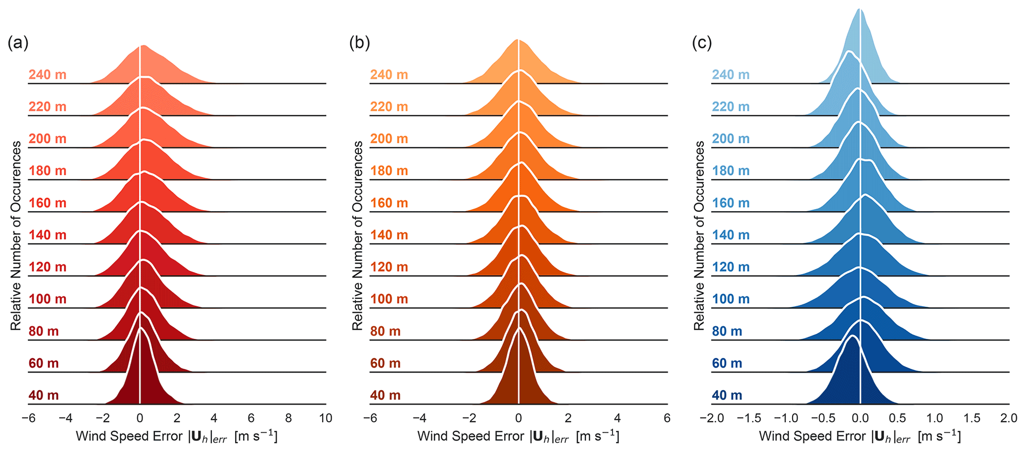
Figure 6 Kernel density estimates of the 1 Hz wind speed error distributions. Errors are computed with respect to the volume average at each height for the (a) strong CBL, (b) weak CBL, and (c) stable boundary layer (BL). Each distribution comprises 108 000 data points.

Statistical moments serve to summarize and quantify the properties of the distributions, facilitating intercomparison and the identification of trends in the error behavior. We consider the first four moments: unbiased estimators of the mean, centered variance/standard deviation, and the adjusted Fisher–Pearson standardized moment coefficients for skewness and excess kurtosis (Zwillinger and Kokoska, 2000; Joanes and Gill, 1998). The mean, μ, represents the expected error, with non-zero values indicating a bias in the lidar observation. The centered variance, σ², measures the spread of the distribution about the mean, though the corresponding standard deviation, σ, can be easier to intuit as an indication of the distribution width and represents typical error magnitude in the original measurement units. For centered (zero mean) distributions, the standard deviation is comparable to the root-mean-squared error (RMSE or RMSD) metric. The higher-order moments of skewness and kurtosis, normalized by the standard deviation, are non-dimensional descriptors of the distribution shape, namely asymmetries and decay of the tails. With a few exceptions, the metrics suggest that the distributions do not differ substantially from normal.

We start by examining the reconstructed horizontal velocity components. The skewness and kurtosis metrics suggest generally normal behavior except for the excess kurtosis (+1) indicating more slowly decaying tails, particularly near the surface. The rest of the discussion of the component errors focuses on trends in the mean and variance; see Appendix A for the first four moments for all variables.

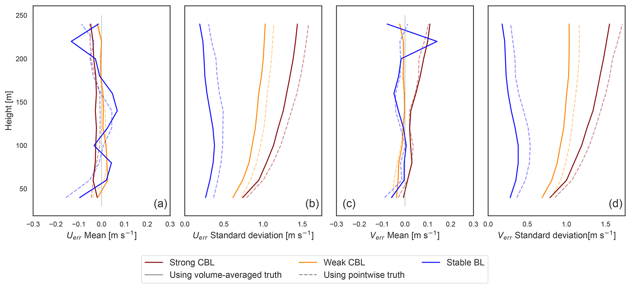
Figure 7 Mean and standard deviation of error in the u (a, b) and v (c, d) horizontal velocity components using both volume-averaged truth (solid) and pointwise “tower” truth (dashed). Stability cases are distinguished by line color.

In all cases, the distribution of the error with respect to the pointwise truth displays a larger standard deviation than the error using the volume-averaged truth (Fig. 7). With the beam measurements at the perimeter of the scan volume, the lidar reconstruction has no way to predict small-scale variations at the center of the volume where the pointwise truth resides. It can only reconstruct an average representation, and comparison with the point value incorporates additional uncertainty into the error.

Figure 8 Contributions to the mean (a, b, c) and variance (d, e, f) of the error for each wind component, partitioned according to Eqs. (12)–(15) into horizontal ($u^{\prime \prime },v^{\prime \prime }$) and vertical (w^′′) velocity perturbations, RWF effects (r), and combined covariance effects.

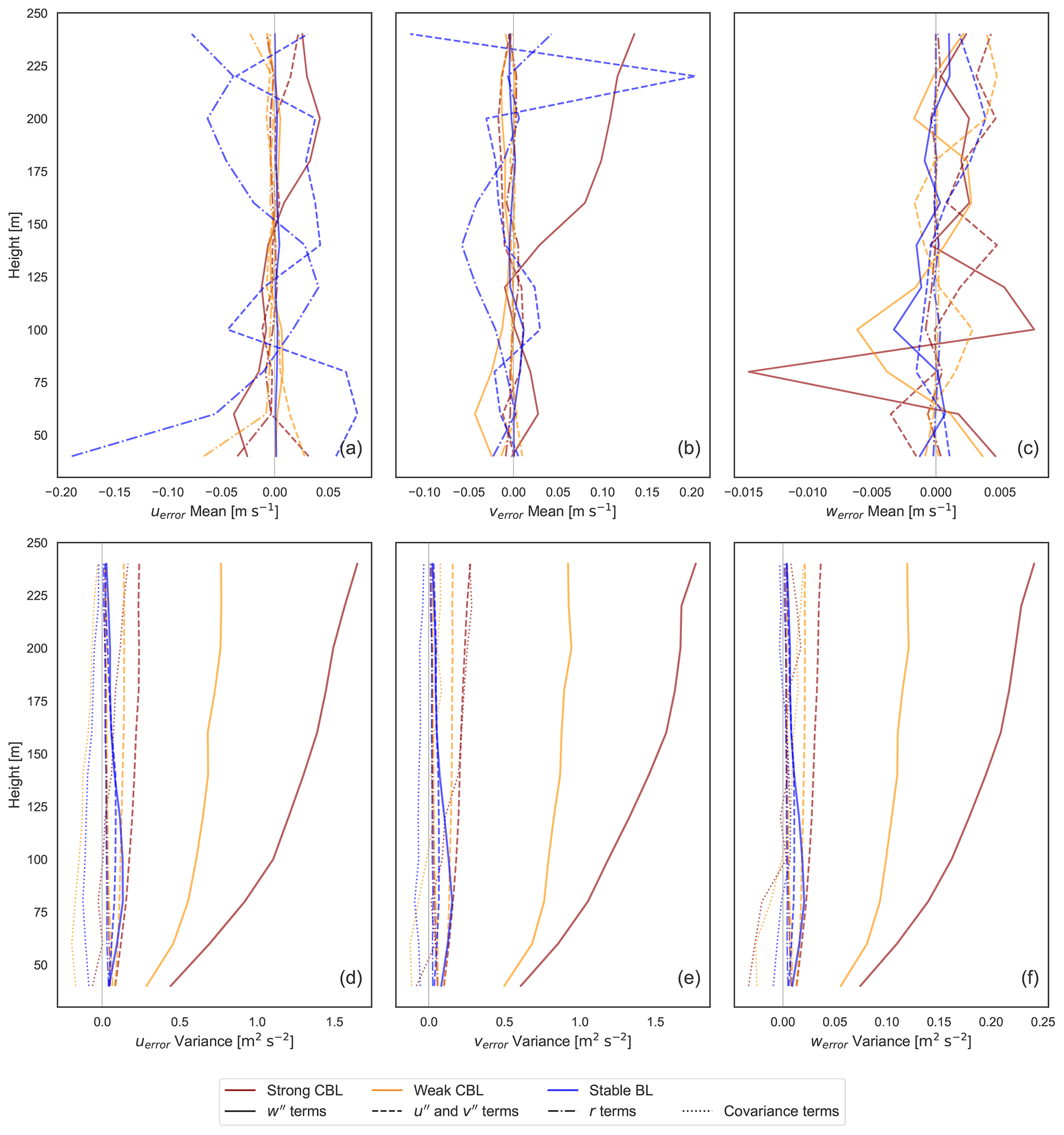
In general, the mean biases are close to zero (<0.05 m s⁻¹) with just a few instances in the stable BL and at the top of the range in the strong CBL exhibiting biases up to 0.15 m s⁻¹. The strong convective case consistently suffers from more significant errors, reflected in the greater error standard deviations (around 1–1.5 m s⁻¹). It is followed by the weak CBL (0.5–1 m s⁻¹), with the stable case being the best behaved (<0.5 m s⁻¹). In the convective cases, the error magnitudes grow consistently with height to the top of the lidar range in the middle of the boundary layer. The stable BL error peaks in the middle of the boundary layer (around 80 m). Using the derived forms for the wind component errors (Eq. 11), we delineate the roles of the perturbations in the horizontal ($u^{\prime \prime },v^{\prime \prime }$) and vertical (w^′′) velocities and due to the RWF in the total error mean and variance (computed from the 45 virtual lidar with no offset from the LES axes) (Fig. 8).

For the most part, in homogeneous turbulence, non-zero mean biases in u and v can be attributed to RWF effects. The largest deviations from zero arising instead from velocity perturbation terms occur in the strong CBL case and stable case (Fig. 8a, b), where coherent structures large enough to span the scan volume (42–255 m) may appear. Repeated sampling across asymmetric internal structures in convective plumes or large turbulent features above the stable BL could potentially induce small biases. In the absence of strong systematic results, however, numerical noise and the finite nature of the ensemble can also induce small apparent deviations in the model that do not meaningfully indicate bias. The bias introduced by the RWF, though also generally small (<0.15 m s⁻¹), is considered robust since it is mechanistically supported.

Figure 9 The mean vertical profiles of (a) $\stackrel{\mathrm{‾}}{u}$ and (c) $\stackrel{\mathrm{‾}}{v}$ from the LES along with the corresponding RWF-weighted view of the profile sampled along the angled beam. (b, d) The RWF-weighting bias on the uniform mean vertical profiles of $\stackrel{\mathrm{‾}}{u}$ and $\stackrel{\mathrm{‾}}{v}$ compared to the bias due to the RWF in the full virtual lidar.

The most prominent influence of the RWF is near the surface layer due to strong shear, manifesting as an under-estimate of the magnitude of the horizontal velocities. As shown for a general RWF (Eq. 16), curvature in the wind profile permits larger measurement biases from the targeted point value. In the LES test cases, the RWF contribution to the mean ensemble error corresponds to the bias of the RWF acting on the background $\stackrel{\mathrm{‾}}{u}$ and $\stackrel{\mathrm{‾}}{v}$ profiles (Fig. 9). The effect is most significant near the surface layer in strong shear (−0.2 m s⁻¹ in the stable BL) and around inflection points. Although the peak curvature of the vertical profile of the weak CBL (about −0.03 m⁻¹ s⁻¹) has a greater magnitude than that of the stable BL (around −0.01 m⁻¹ s⁻¹), the curvature in the stable CBL is more sustained and paired with larger wind speeds, which leads to a larger realized bias (Eq. 16). Our findings are consistent with previous studies that have identified the key interaction of the RWF with shear, resulting in error bias (Lindelöw et al., 2008; Clive, 2008; Courtney et al., 2014).

The variability of the measurement errors, shown in the variance and standard deviation, is a consequence of the velocity perturbations, with negligible contribution from the RWF. In convective conditions, the weighted vertical velocity perturbations dominate the other sources of variance in the error, indicating the w^′′ terms are dwarfing the others and driving the error (Fig. 8d, e). The stronger the convection, the stronger the effect, echoing the findings by Rahlves et al. (2021) that the bulk error is larger in more strongly convective conditions. By contrast, the error in the stable BL arises from a more even interplay of the horizontal and vertical velocity perturbation terms. The covariances between the beam perturbations generally serve to temper the overall error variances, particularly near the surface where the smaller scan volume may permit stronger correlations.

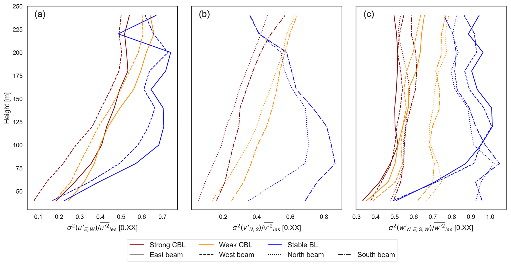
Figure 10 The proportion of the full turbulent velocity variances ($\stackrel{\mathrm{‾}}{{u^{\prime }}^{\mathrm{2}}},\stackrel{\mathrm{‾}}{{v^{\prime }}^{\mathrm{2}}},\stackrel{\mathrm{‾}}{{w^{\prime }}^{\mathrm{2}}}$) present in the variance of the turbulent perturbations from the lidar scan-volume average (e.g. ${\mathit{\sigma }}^{\mathrm{2}}\left(u_E^{\prime \prime }\right)$). Ratios shown using the perturbation variances at each beam.

The velocity perturbation terms arise from a weighted, filtered portion of the full turbulent velocity variance. Physically, we might expect convective plumes to violate horizontal uniformity in the flow (Fig. 4), but it is an even more outsized effect that creates the error in convective conditions. The convective plumes induce large but localized vertical velocity variations, much of which are not filtered out by the lidar scan volume, the diameter of which ranges from 42–255 m (Fig. 10). The cone angle then over-weights the vertical velocity variance terms (Eq. 11). The compounding effects conspire to make the vertical velocity dominant in creating large errors in convective conditions (Fig. 8d, e, f). Even in the stable BL, the vertical velocity perturbations contribute significantly to the error. The smaller length scales of the vertical velocity turbulence in stable conditions coincide with smaller turbulent variance, but also allow a larger portion of the variance to be filtered through the lidar scan volume (Fig. 10). The result is again over-weighted according to the cone angle. The horizontal velocity variances, meanwhile, are filtered out to a greater degree by the scan volume and are not weighted in the error form, lessening their relative impact compared to the vertical velocity terms.

The coupling of the error with the turbulent structure, and the vertical velocity in particular, helps explain the cause of the correlation of the error height trends with the boundary layer structure. The error variance in the stable boundary layer peaks near the center of the boundary layer where the turbulent vertical velocity variances are large and more of the horizontal variances pass through the filter. The diminishing error variance at higher altitudes relies on the decay of both the horizontal and vertical perturbations and the increase in turbulent length scales, which combats the increase in scan volume size. The lidar range does not extend to the top of the boundary layer in the convective test cases, but we might expect the error variance to also peak in the middle of the boundary layer and decrease with height as the vertical velocity variance tapers back toward zero. The dependence of the error height trends not only on the volume circumscribed by the scan but also on the vertical structure of the boundary layer and corresponding scale and character of the turbulent structures was also noted by Wainwright et al. (2014) for sodar measurements.

The choice of cone angle determines the degree of projection of the horizontal and vertical perturbations (manifest in the weighting in the error form) as well as the spatial separation of the sampling beams. In the strong and weak CBL test cases in particular, the error demonstrates the adverse impacts of heavy weighting on the vertical perturbations. Rahlves et al. (2021) tested a low elevation angle (35.3^∘ from Teschke and Lehmann, 2017) with a virtual instrument in quasi-homogeneous convective conditions with favorable results compared to more typical larger elevation angles (60, 75^∘). Improvements achieved by reducing the angle to lessen the weighting on the vertical velocity perturbations, however, may be offset by the corresponding effects of increasing the separation of the beams. In quasi-homogeneous turbulent conditions, a lower elevation angle lengthens the filter scale, allowing for larger error variances, up to a cap determined by the full, unfiltered turbulence. The optimal cone angle to minimize the error will depend on the balance of the competing effects in a particular flow.

3.2 Raw 1 s horizontal wind speed and direction

The horizontal wind speed and direction are computed from the lidar-measured wind components and compared against those of the volume-averaged winds (Eq. 17). The errors (Eqs. 18 and 21) exhibit behavior consistent with theoretical expectations (Sect. 2.3.4).

The distributions are again roughly normal. There is a slight positive skewness (long tail on the positive side of the distribution) in the wind speed error (0.25 in strong convection) (Fig. A2), likely due to the positive second-order bias term (Eq. 18). The bottom range gates, influenced by the surface layer, also deviate from normal under strong convection: there is evidence of slight positive skewness (0.4) at the surface in wind direction. The excess kurtosis (+1–2) again suggests more slowly decaying tails, more pronounced near the surface. Wind direction at the surface exhibits the most extreme behavior, with an excess kurtosis of +8 at the surface.

Figure 11 Mean and standard deviation of error in the 1 Hz vector-averaged wind speed and wind direction. For wind speed, the primary axis gives absolute error, and colored secondary axes designate relative error with respect to 100 m values for the respective LES case.

The height and stability trends in the mean and variance of the errors (Fig. 11) follow from those of the horizontal velocity components (Fig. 7). The standard deviation of the wind speed error corresponds to that of the horizontal components as anticipated, carrying over the larger error magnitudes in the strong CBL compared to the weak CBL and followed by the stable BL. The trends in standard deviation, growing with height over the lidar range in the convective cases and peaking mid-boundary layer in the stable BL, are also consistent with those of the u and v component errors. The bias in the u and v components also propagates into the bias in the wind speed error, reflecting the underestimate due to shear near the surface of the stable BL and weak CBL.

We derived a systematic positive bias term in the wind speed measurement (Eq. 18) that is leading order when the biases in u and v are negligible. In the ensemble mean, it is proportional to the variance of the horizontal component errors and inversely proportional to the wind speed (Eq. 19). It follows that measurements in the strong CBL experience the most significant biases (0.2–0.4 m s⁻¹), growing with height as do the u and v error variances. The same occurs, to a lesser degree, in the weak CBL with a bias <0.2 m s⁻¹. In the stable BL, which has small u and v error variances and fast mean winds, the bias term becomes negligible.

We anticipated that the wind direction bias should be close to zero assuming the u_err and v_err were similarly distributed with zero mean. The computed bias is indeed generally small (<0.5^∘ in the weak CBL and stable BL and <2^∘ in the strong CBL). Under strong convection, the wind direction observations list more and more counterclockwise (southward) from truth with height. The expansion of the expected bias in the wind direction (Appendix B) relies on the uniform distribution of the direction and magnitude of the horizontal error vector (u_err,v_err)^T, which coincides with zero mean bias in the horizontal wind components. Deviations from this assumption result in small terms scaled by powers of $\mathrm{1}/\left|{\mathit{U}}_h\right|$ (Eq. B9) so that fast wind speeds act instrumentally to diminish bias in the wind direction. The combination in the strong convection case of the coherent structures and the weak winds allows even small non-zero means in u and v to be amplified to create the wind direction error bias. The stable BL, on the other hand, tempers wind direction bias through the strength of the wind speeds. Over an ensemble including instruments spanning a full 360^∘ set of offsets, we would expect the signs to cancel, leaving zero bias. Within the ensemble of offsets over a 45^∘ arc used here, however, the signs are consistent, and the bias persists across the rotated lidar measurements. Measurements made in conditions of slow winds of fairly consistent direction, as in the strong CBL case, do not benefit from the cancellation expected in an ensemble over all instrument orientations and should take into account the possibility of a persistent bias arising in the wind direction.

3.2.1 Effects of wind speed and orientation angle

The idea that lidar might manifest a smaller error at higher winds seems intuitive. In addition to potential implicit effects on correlations across the scan volume, the derived error forms (Eqs. 18 and 21) draw out explicit dependencies on wind speed and direction. We find that wind speed powerfully influences error in the lidar observations, whereas the orientation of the lidar with respect to the mean wind has a negligible impact.

Figure 12 Trends in (a) wind speed and (b) wind direction errors with respect to the volume-averaged wind speed. Data points from all lidar measurements are colored by stability case: strong CBL (red), weak CBL (orange), and stable BL (blue). Reference lines are given for the mean error for each stability at each wind speed (colored, dashed). Reference lines (grey, solid) trace (a) $\mathrm{1}/\left|{\mathit{U}}_h\right|$ decay and (b) the $\mathrm{1}/\left|{\mathit{U}}_h\right|$ and $\mathrm{4}/\left|{\mathit{U}}_h\right|$ envelopes.

The wind speed trends across all the virtual lidar wind speed and direction data are shown in Fig. 12. The wind speed error magnitudes visibly contract from the slow, strong CBL data to the fast winds of the stable BL; the decrease has to do with the identified mechanisms of filtered turbulence driving the error variance in each of the stability regimes. A trend line for the mean error in the wind speed measurement is computed for each stability case with respect to the true volume-averaged wind speed over 0.5 m s⁻¹ bins with at least 2500 points. The positive bias in each stability case is clearly evident. All else being equal, we expect from the form of the wind speed bias (Eq. 19) that faster wind speeds should temper the magnitude of the bias according to $\mathrm{1}/\left(\right|{\mathit{U}}_h\left|\right)$. Comparing the tending bias with the expected decay, we cannot confirm the behavior empirically over the natural variations in the error variances concomitant with wind speed in the virtual lidar test case data.

According to the wind direction error form (Eq. 21), we expect the magnitude of the error to decay on the whole with at least $\mathrm{1}/\left|{\mathit{U}}_h\right|$. Indeed, allowing for potentially different scales of u and v error in the numerator, the data fall nicely along the reference envelopes, especially along the tail of the stable BL. In some cases, the decay in the error magnitudes is greater than the anticipated $\mathrm{1}/\left|{\mathit{U}}_h\right|$ bound. This may be in part because the inverse tangent in the full error expression (Eq. 21) should act to further curtail the size of the largest errors more than is captured in the bounding estimate (Eq. 22) and in part because of implicit correlation effects and variance behavior with height and wind speed.

Potential differences in error as a function of the lidar orientation are due to projection of the error vector onto the mean wind parallel or transverse directions (Eqs. 18 and 21) and implicit differences in correlation effects in the streamwise and cross-stream directions. In the virtual lidar error data, only small discrepancies could be distinguished between errors in the streamwise and cross-stream velocity component estimates; comparing the disaggregated rotated lidar ensembles (Fig. 7), a slight amplification in error variance shifts from one component to the other.

Figure 13 Errors in the 100 m (a) wind speed, (b) wind direction, and (c) vertical velocity (wind direction weighting, Eq. 9) in the stable BL case plotted against the offset angle between the wind direction and the nearest lidar axis. Lines show the means (solid) and standard deviation interval (dashed).

As in Rahlves et al. (2021), our results suggest that a change in orientation has a negligible effect on the error that is washed out by other more significant effects (illustrated by the 100 m measurements in the stable case, Fig. 13). The noticeable trend with offset angle in the vertical velocity error appears only when using the wind direction weighting (Eq. 9), not under equal weighting of the beams (Eq. 8). As discussed in Sect. 3.4, the dependence is likely due to the difference in the effective number of beams used, with an average over two beams having more variability than over four. The lack of sensitivity in the wind speed and direction error distributions suggests that the direction of the error vector, (u_err, v_err)^T, is fairly evenly distributed. Comparing moments across the rotated ensembles (Fig. A2) confirms that there is little meaningful difference in the error behavior between offset angles (with some exception for peak variance of the stable BL vertical velocity error). It should be noted that although no strong trends were found with respect to the relative offset between the mean wind and the lidar axes, the signs of some of the biases can change with the signs of u and v.

3.3 Time-averaged horizontal velocities

Common time-averaging intervals used with lidar data may be over 2, 10, or even 30 min, with experimental evaluations of the system accuracy often reported in terms of the 10 min average in wind energy contexts. As with the error in the high(er)-frequency wind measurements, we characterize the error distribution of the 10 min averaged measurements (Fig. 14).

Figure 14 Mean and standard deviation of error in (vector) 10 min averaged wind speed and wind direction. For wind speed, the primary axis gives absolute error, and colored secondary axes designate relative error with respect to 100 m values for the respective LES case.

We first characterize the error distributions of the vector-averaged lidar measurement compared to the vector-averaged point and volume references for the wind speed and direction (Fig. 14). Each distribution in the 10 min average comprises an ensemble of a total of 180 values (ensemble and offset angles).

Under stationary and homogeneous flow conditions, the notions of pointwise and volume-averaged truth start to converge to a general spatiotemporal average, which is reflected in the merging of the two error distribution profiles. The correspondence suggests that field studies comparing against time-averaged “point” tower measurements can effectively reflect the error with respect to the volume average as well (ignoring spatial displacement of the tower from the lidar). The overall error magnitudes found by the virtual lidar are consistent with those in field deployments of lidar compared against tower measurements. In select flat conditions typical mean discrepancies in the range ±0.2 m s⁻¹ with standard deviations of 0.20 m s⁻¹ (Courtney et al., 2008) have been reported, which encompass all but the more extreme errors in the strong convection case. The virtual 10 min averaged wind speeds have mean errors within ±0.2 m s⁻¹ with standard deviation <0.3 m s⁻¹. Furthermore, the wind direction has mean error bias within 2^∘ and standard deviations within 2.5^∘, except for in the strongly convective case where it can reach up to 12^∘.

As anticipated, the time-averaged errors reflect a decrease in the wind speed bias in the convective cases, little change in the wind direction bias, and a reduction of the standard deviations (by a factor of around 5). The degree of reduction in the biases and standard deviation is not uniform, but varies somewhat with stability and height, likely depending on the decorrelation scales in the error time series. This leads to some shift in the shape of the moment profiles compared to the original distribution, e.g. the curvature of the standard deviation with height.

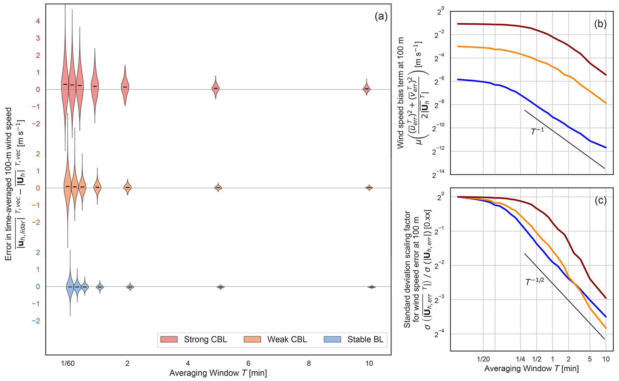
Figure 15 Wind speed error at 100 m under a vector time average. (a) A violin plot of the error distribution and mean for each stability over several averaging windows up to 10 min. (b) The reduction in the second-order positive bias term against a reference T⁻¹ rate. (c) The reduction in the error standard deviation against a reference $T^{-\mathrm{1}/\mathrm{2}}$ rate.

Based on the error model, not only a reduction in error magnitude and bias (in the wind speed) were predicted, but also the rate of reduction. The wind speed error distribution at 100 m was computed for several time-averaging windows ranging from a few seconds to the full 10 min span available. Not only is the reduced spread of the distribution marked across cases and the decay of the bias apparent in the strong CBL (Fig. 15a), but both decay according to the anticipated power laws ($\propto T^{-\mathrm{1}}$ decay of the bias term and $\propto T^{-\mathrm{1}/\mathrm{2}}$ reduction in the standard deviation (Fig. 15b,c)). The behavior is representative of other heights and of the decay rate in the standard deviation of the wind components and wind direction averages.

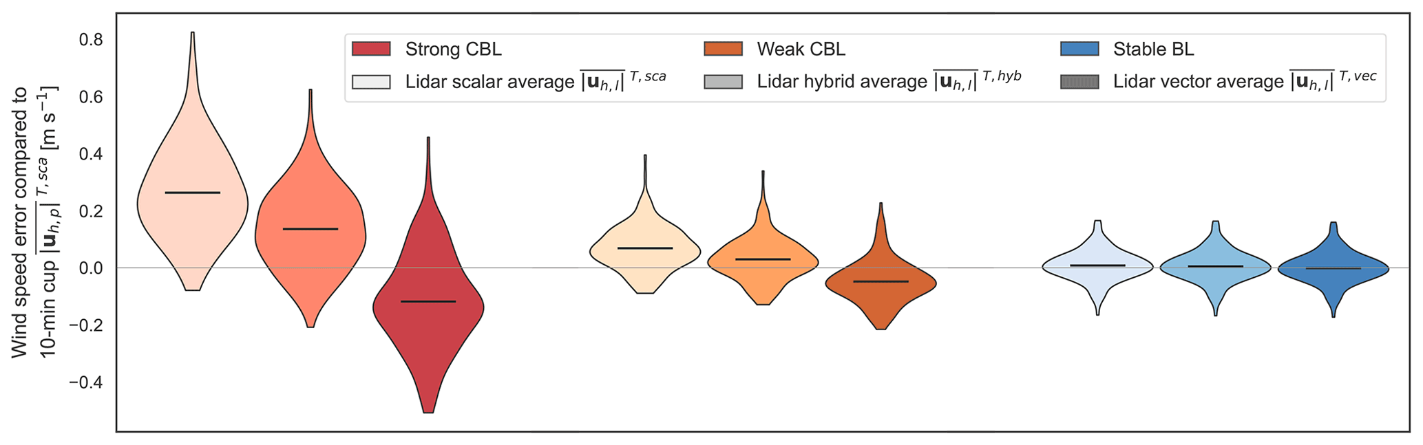
Figure 16 Comparison of time-averaged lidar wind speed estimates at 100 m (using vector, scalar, and hybrid average) with the pointwise scalar average representing a cup measurement. Black horizontal lines show the distribution means.

We also compared 10 min vector-, scalar-, and hybrid-averaged lidar wind speeds (Eqs. 26, 27, and 33) against a scalar-averaged point measurement made at the center of the scan volume for the 100 m winds (Fig. 16). At this height, which is mid-boundary layer in all stability cases, the lidar scalar average over-estimates the speed reported by the “cup” measurement whereas the vector average under-estimates the speed. The straddling of the cup measurement was anticipated for unstable stratification or cases of strong mechanical turbulence. The hybrid scheme, taking the weighted average, works as designed to scale the inflation of the lidar scalar-averaged winds compared to the vector average to better represent the inflation experienced by a point measurement, thereby improving the error bias. The reduced bias is most pronounced in the convective cases, which experienced larger biases compared to the cup measurement in both the vector and scalar averages and a larger gap between the two averaging types. The bias in both average types is small in the stable BL so that the realized change is negligible. We now consider what the ideal weights for a hybrid scheme would be, across the simulated cases and heights, and how they relate to the flow behavior.

The theory behind the hybrid average leverages the expected inflation in a scalar-averaged wind speed (compared to the vector average) in a lidar and a pointwise measurement (Eqs. 32 and 31). A pointwise inflation arises purely from fluctuations in the horizontal velocities ($u^{\prime },v^{\prime }$) while the lidar measurements of u and v contain projected vertical velocity fluctuations, which are also reflected in the inflation factor. We decompose the contributions to the lidar inflation factor based on the virtual lidar ensembles and compare to the corresponding pointwise inflation (Fig. 17). Following the form of the analysis in Rosenbusch et al. (2021), the two-point beam average is used as the U and V truth reference in the lidar computation, and the RWF is omitted (instead directly interpolating the radial velocity) to focus on the turbulence effects.

Figure 17 Decomposition of the lidar and pointwise scalar-average inflation factor (α_l and α_p) in the (a) strong CBL, (b) weak CBL, and (c) stable BL. Contributions to the inflation from horizontal ($u^{\prime },v^{\prime }$), vertical (w^′), and cross terms $(u^{\prime }{w}^{\prime },v^{\prime }{w}^{\prime })$ with the lidar shown in color and the pointwise inflation in grey. (d) The ideal weighting for the scalar-averaged lidar measurement in a hybrid scheme computed from the ratio of pointwise inflation factors and solved directly from the 10 min averaged mean errors.

The lidar wind speed inflation is decomposed into horizontal velocity fluctuation terms and terms due to vertical or mixed vertical–horizontal velocity fluctuations. Note that the lidar inflation factor is due to perceived variances in the horizontal velocity components, and its decomposition echoes the decomposition of the u and v error variances (Fig. 8). The findings are consistent with the analysis of limiting-case behavior in Rosenbusch et al. (2021). The combined contribution to the lidar inflation factor by the horizontal velocity fluctuations is consistently less than that experienced by a point measurement (across stability and height). Based solely on these terms, the lidar-scalar average would under-estimate the averaged cup wind speed. The additional variation due to the vertical velocity, which has no counterpart in the point measurement, means that in the convective cases the lidar scalar average experiences a greater inflation than a cup measurement would. The stable BL behaves in a similar fashion within the bulk of the boundary layer (<150 m) where there is moderate vertical velocity variance. Higher, however, the vertical velocity contributions become less substantial and only just compensate for the difference between the lidar and pointwise horizontal velocity terms. In this upper regime, the cup measurement would be expected to match or exceed the lidar scalar average. The ideal weighting of the lidar scalar average for the hybrid scheme (assuming the vector-average biases are zero) is given by the ratio of the pointwise to lidar inflation factors, ${\mathit{\alpha }}_{\mathrm{p}}/{\mathit{\alpha }}_{\mathrm{l}}$. The ratio determined from the LES test cases (Fig. 17d) suggests a value smaller than two-thirds is needed to fully counter the vertical velocity contribution in the convective conditions (around 0.3–0.6). A larger weight would be required in stable conditions: 0.7 up to 1 in the bottom portion of the boundary layer and exceeding a weight of 1 where the lidar scalar average underestimates the point scalar average. Overall, without optimizing the weighting for a particular type of flow, the two-thirds weight splits the difference between the LES test cases.

The derivation of the hybrid scheme and the weightings shown above are predicated on the assumption that the bias term vanishes completely in the 10 min vector-averaged pointwise and lidar measurements. The vector averages were assumed to be equal approximations of the speed of a Reynolds-averaged wind. The behavior of the bias in the vector-averaged winds suggests that, at least for the upper range gates in the strong CBL, a non-negligible positive bias (0.1–0.2 m s⁻¹) persists under a 10 min average (Fig. 14a). The persisting bias results from the combination of a large initial bias (Fig. 11a) and correlation in the time series slowing the decay of the bias term under the vector average (Fig. 12). In the derivation, the difference between the vector and scalar time average is assumed to reflect the entire inflation factor; however, in conditions such as the upper strong CBL, only a portion of the inflation factor divides the two after 10 min. The 10 min lidar scalar average will consequently be over-weighted when using the ${\mathit{\alpha }}_{\mathrm{p}}/{\mathit{\alpha }}_{\mathrm{l}}$ ratio. Again omitting the RWF from the model, we solved for the weights required to fully cancel the bias in the lidar–cup comparison using the ensemble errors of the 10 min averaged winds (Fig. 17d). We have omitted the weights for the stable BL; the small biases, <0.02 m s⁻¹, produce noisy, unreliable results, and the vector-average bias in this case has decayed to negligible levels. In practice, the 10 min averages in the strong CBL require smaller weights (0–0.4) on the lidar scalar-averaged wind speed than expected based on the full inflation factors (0.3–0.6). In order for the underlying theory in the weighting to be applied in this case, the remaining inflation in the vector-averaged wind speed would have to be addressed directly or further diminished by extending the time window.

3.4 Vertical velocity measurements

The vertical velocity measurement demands separate treatment from the horizontal winds. The vertical velocity itself behaves distinctly from the horizontal winds because it varies more rapidly, and the features of interest occur at smaller spatial and temporal scales, with the background (spatiotemporal average) signal tending close to zero. The WindCube V2 offers two possibilities to reconstruct the vertical velocity from the measured radial velocities by either equally weighting the beams or using the wind direction to selectively weight them (Eqs. 8 and 9). Because the variation in the vertical velocity generally occurs at a smaller scale than the scan volume, much of the dynamics will tend to be lost in the reconstruction process. Even if the volume average were perfectly recovered, the average itself loses information. The measurement from the vertical beam is a third option that samples just the vertical velocity and does not require reconstruction.

Figure 18 shows the mean and variance of the error using the two reconstruction techniques. The vertical velocity error distributions using point and volume-averaged truth references do not mirror one another as they do for the u and v velocities. Because the variability in vertical velocity occurs on a shorter length scale, the pointwise value is less representative of the volume average, which explains the greater discrepancy. In all cases, the bias is negligible (<0.02 m s⁻¹). The standard deviation of the error is driven by similar dynamics as in the horizontal components; the vertical velocity variance dominates and the height trends follow the boundary layer structure (Fig. 8). In the vertical velocity, however, the relative magnitude of the standard deviation can grow to large fractions (0.3–0.9) of typical magnitudes in all stability cases, obscuring the actual signal in the measurement.

Figure 18 Comparison of the error in vertical velocity measurement using the evenly weighted vertical velocity reconstruction (Eq. 8, dotted line) and the wind-direction-weighted reconstruction (Eq. 9, solid line). Both use the volume average as truth.

Comparing the reconstruction techniques, at least with respect to the disk-averaged truth, the lessened dependence on the full four beams using wind direction weighting seems to outweigh the beneficial effects. When the wind is directed between the lidar axes (45^∘ offset), the two reconstructions are identical; the difference arises when the wind direction lies more closely with one of the axes so that two beams are weighted more heavily, shrinking the contribution from the other two beams. In our test cases, the reconstruction relies primarily on the east and west beams. With respect to the volume-averaged vertical velocity, the standard deviation of the error is on the whole larger under the reconstruction using wind direction weights than with equally weighted beams (Fig. 18b). The behavior is consistent with the sensitivity of the wind direction weighting to the orientation angle of the instrument (Fig. 13), which showed slightly smaller standard deviations when the mean wind was closer to a 45^∘ offset with the lidar axes.

In the context of the random variable error model (Eq. 11), weakening or removing dependence on some of the beams removes the chance for canceling the perturbations; the mean over two points will tend to be a poorer representation of the volume average than the mean over four points. The concentrated dependence can also magnify the influence of variations experienced at the two beam locations. In light of the empirical error behavior, the benefits of incorporating more points seem to supersede the benefits of streamwise correlations.

The vertical beam sidesteps the implicit volume average along with the need for any reconstruction. In this case, the error incurred in measuring a pointwise vertical velocity arises purely from the effects of the range-gate weighting in the measurement process. The RWF produces errors with magnitude and character that are distinct from the reconstruction errors (Fig. 19). Across stability cases, the bias is negligible (<0.005 m s⁻¹). The difference in standard deviation between the convective cases vanishes, and the overall magnitude is significantly reduced compared to that in the reconstruction methods. As opposed to the error in the reconstruction estimate, the standard deviation with only the RWF decreases with height. In the stable case, the RWF was a larger relative portion of the error in the vertical velocity reconstruction (Fig. 8). Under stable conditions, the difference between the reconstruction and the vertical beam is less dramatic; the standard deviation magnitudes are about halved, and the decrease in the standard deviation with height exists with both but is more pronounced with the vertical beam. Even when using the vertical beam, the standard deviation can still be relatively quite large compared to typical values.

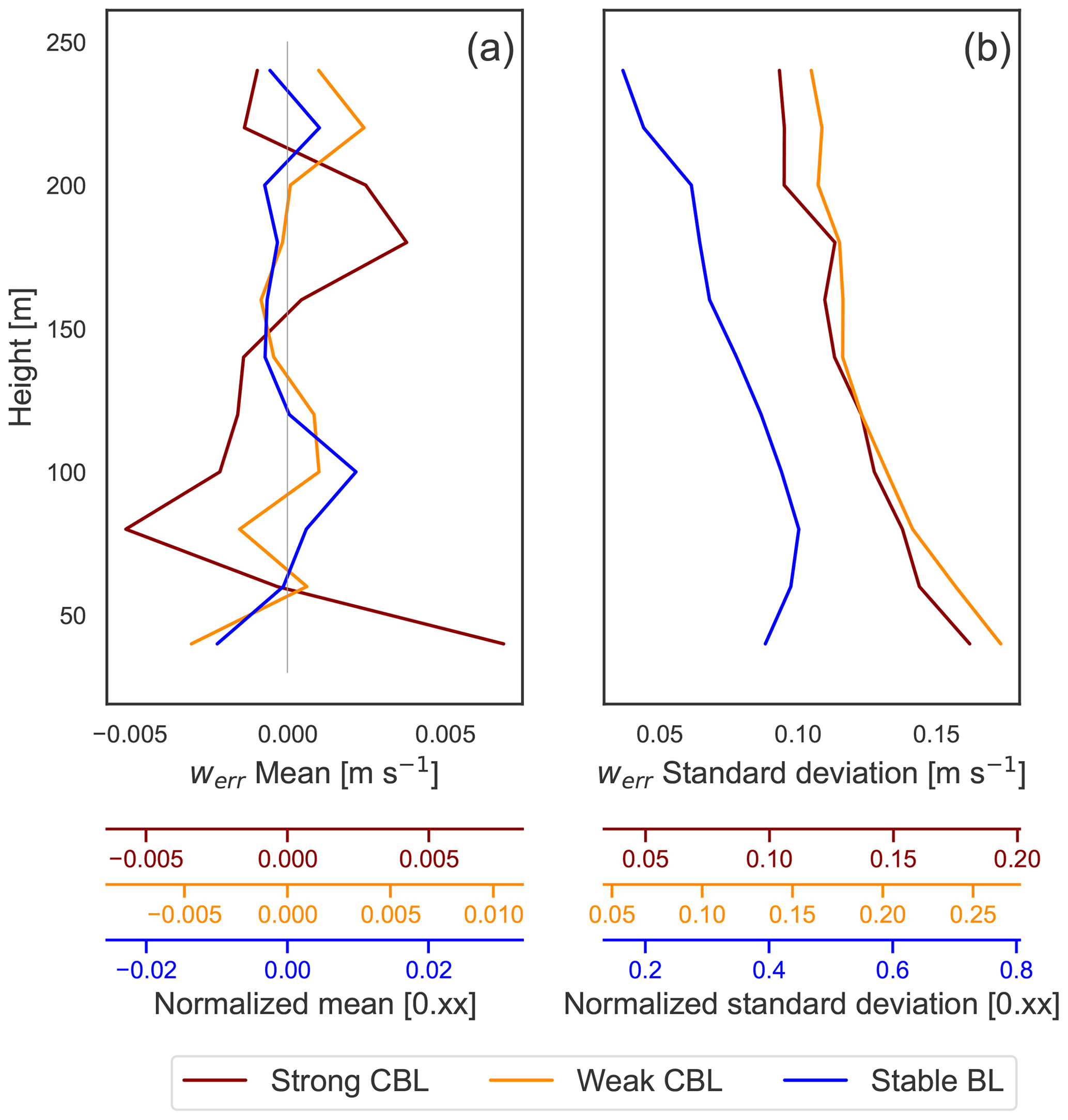
Figure 19 Vertical velocity measurement error moments for the vertically pointed beam. Error is with respect to the pointwise truth.

4 Discussion

The quantification of the error found here aligns with values found in field studies (Courtney et al., 2008) and in similar estimates of virtual lidar performance in baseline convective conditions (Rahlves et al., 2021). To define the error, we compared virtual measurements against both a pointwise truth reference and the average over the scan volume. With 10 min averaging, the distinction between the kinds of spatiotemporal averages fades, and the two error distributions seem to converge. The magnitudes of the overall errors in the virtual measurements fall generally within experimentally determined ranges in favorable conditions: 10 min averaged wind speeds have mean errors within ±0.2 m s⁻¹ with a standard deviation of less than 0.3 m s⁻¹, and wind direction has a mean error bias within 2^∘ and standard deviations in 2.5^∘ except for the strongly convective case where it can reach up to 12^∘.

The character of the error in the reconstructed wind vector components is driven by the form of the turbulence, so that the lidar accuracy is dependent on the flow regime and vertical structure of the boundary layer. Our derivation explains findings from other sensitivity studies (Klaas and Emeis, 2022; Rahlves et al., 2021) in that unstable conditions are prone to larger errors than stable conditions. The error variances derive from weighted, spatially filtered turbulent variances in the horizontal and vertical velocities. The vertical velocity variances are of particular importance. Because the variations in vertical velocities tend to occur on smaller spatial scales, fewer of these variations are filtered out by the lidar scan volume scale. The resulting velocity perturbation variance is then weighted more heavily in the error than horizontal perturbations, i.e. the “projection” of the vertical velocity variations is greater on a more narrow scan cone. In convective conditions, the compounding mechanisms lead to vertical velocity perturbations almost single-handedly accounting for the error. Under stable conditions, the error magnitudes are notably smaller and result from a more balanced interplay of the vertical and horizontal velocity inhomogeneities. Previous work has investigated the relationship of lidar error with aggregate turbulence intensity (Courtney et al., 2014). Our findings reflect the connection, with additional separation of the turbulent fluctuations into each of the components to allow for the difference in spatial scales and weighting to come through.

The range-gate weighting in the radial velocity measurement has minimal relative effect on the total lidar error except in high-shear regions near the surface layer. Deviations incurred in the radial velocity measurement by the weighted volume average along the beam should vanish under constant gradients but can grow in the presence of large second derivatives in the radial velocity projection along the beam. For the most part, the impact of the larger variations over the scan volume dominate any RWF effects. In the bottom few range gates near the surface, however, the virtual lidar data reflect a prominent interaction of the RWF with shear near the surface layer, leading to measurement bias. The persistent curvature in the profile results in significant (around 0.2 m s⁻¹ in the stable case) and consistent under-estimation of the magnitude of along-wind horizontal component(s). Our findings are consistent with previous studies that have identified the key interaction of the RWF with shear resulting in error bias (Lindelöw et al., 2008; Clive, 2008; Courtney et al., 2014).

Within the class of DBS and VAD profiling scans, any control over the reconstruction error comes from adjusting the cone angle, ϕ, and the number and spacing of the scan azimuthal angles, {γ_i}. The virtual instrument tests in our study held these parameters fixed to match the WindCube V2, but other studies have explicitly investigated the sensitivity of the lidar error with respect to the scan configuration. The decomposition of the error in our study according to the derived error form, however, allows for insights into the relative impacts of the configuration choices on the error behavior.

The cone angle determines the degree of projection of the horizontal and vertical perturbations (manifest in the weighting in the error form) as well as the spatial separation of the sampling beams. In the strong and weak CBL test cases in particular, the error demonstrates strong adverse impacts of resulting heavy weighting on the vertical perturbations. The dominance of the vertical perturbation terms can be tempered by reducing the elevation angle. Teschke and Lehmann (2017) proposed a shallow elevation angle (ϕ≈35.26^∘) based on an analytic minimization of reconstruction error in a horizontally homogeneous and stationary wind field. Rahlves et al. (2021) tested the low elevation angle with a virtual instrument in quasi-stationary convective conditions with favorable results compared to more typical larger elevation angles.

Some profiling scans use a different number of off-vertical beams to diagnose the mean winds. The beams are usually preferred to be symmetrically spaced to remove potential bias (Sathe et al., 2015; Teschke and Lehmann, 2017). Common reconstructions of the 3D velocity fit sinusoids to the radial velocity measurements using a least-squares process (Newsom et al., 2015). The result is a linear operation on the beam radial velocities of which the DBS scan presented in this study is a special case. The error in these alternative profiling scans should take on a similar error form to that derived here, with perturbations averaged over a greater number of beams. Under a simple stochastic model, Teschke and Lehmann (2017) showed the standard deviation of the error should be proportional to $N^{-\mathrm{1}/\mathrm{2}}$, with N representing the number of beams. The form of the error model also suggests that a greater number of independent samples in the scan volume should help reduce error. We do not explicitly account for the time required to complete the scan, which increases with the number of beams and can become significant. Rahlves et al. (2021) tested scans using different numbers of beams without finding a universal trend in error.

The error in wind component reconstructions propagates into the error in the corresponding computation of horizontal wind speed and direction. The error was formulated in terms of the u and v reconstruction errors. A systematic positive bias in the wind speed estimate emerges from a strictly positive term that scales with u and v error variance and inversely with wind speed, which is corroborated by the virtual lidar data. These findings of a systematic positive bias do not contradict the mechanisms of possible wind speed under-estimation studied in Bingöl et al. (2009) and will coexist with the other competing sources of bias arising from gradients in the flow. The standard deviation of the wind speed error is estimated to be on par with the u and v error standard deviations.

The wind direction has no explicit bias except that arising from the u and v reconstructions. The standard deviation is roughly that of the u and v errors over the average wind speed (i.e. the error magnitudes are reduced at higher winds). The observed error magnitudes strongly depend on mean wind speeds (especially the wind direction) but are only weakly related to the relative orientation of the lidar. As in Rahlves et al. (2021), our results suggest no predominant direction of the random (u_err,v_err)^T vector.

Individual measurements can suffer from larger errors, which can be reduced through time averaging. While time averaging cannot correct for biases in the wind component measurements, the standard deviations of the error are reduced by a factor proportional to $T^{-\mathrm{1}/\mathrm{2}}$, thus also reducing the standard deviation of the wind speed and direction errors. The longer the decorrelation time in the error time series, the less the reduction. The use of both scalar and vector time averaging on wind speed measurements has elicited interest (Courtney et al., 2014; Clive, 2008); Rosenbusch et al. (2021) examine the behavior of pointwise and lidar scalar and vector averages to motivate a hybrid averaging scheme to mitigate the bias of the lidar compared to scalar-averaged cup measurements. We find that the hybrid scheme does improve the bias as designed in many conditions (with exceptions where we might expect the theory to break down, e.g. in the top of the stable BL where vertical velocity variances are close to zero). The ideal weighting to cancel the turbulence effects in the LES test cases, assuming no bias in the pointwise versus lidar vector averages, shifts as expected by stability case. The scalar average would be more heavily weighted in convective conditions and more lightly in stable conditions compared to the current scheme (weight of two-thirds). The assumption of negligible bias in a 10 min vector average does not universally hold across the test cases. The bias is expected to be reduced by a factor proportional to T⁻¹ under the vector average, but in regions with high initial bias and longer decorrelation times (such as the upper strong CBL), positive biases larger than 0.1 m s⁻¹ do persist after a 10 min average. A longer time average is required in such cases for the weightings in the hybrid scheme to be optimal.

Vertical velocity, with features of interest existing on smaller spatial and temporal scales, is a greater challenge to lidar measurements. A vertically pointing beam omits the need for reconstruction or the implicit large-scale spatial average over the scan volume. Instead, only the smaller-scale averaging from the range gate is applied. The errors associated with the vertical beam with respect to the pointwise values are significantly smaller and represent a more useful value that captures more of the small-scale variability in w.

5 Conclusions

Atmospheric variability influences error in wind lidar measurements. By using virtual instruments acting on LES flow fields, error mechanisms can be isolated and explicitly tracked and analyzed to better understand the error behavior as a whole. In this study, we considered profiling lidar measurements in quasi-stationary, quasi-homogeneous conditions. Even in the absence of explicit sources of inhomogeneity, observation error emerges, tightly coupled to the character of turbulence in the flow. The error distributions of a virtual WindCube V2 lidar performing a DBS scan were estimated from ensembles of virtual instruments run in uniform, ideal WRF-LES scenarios in convective and stable boundary layer regimes. An analytic error model leverages random variable representations to describe how the turbulent variability propagates into the lidar error, decomposing the contributions from velocity perturbations at each beam from the volume average and from deviations in the point measurement due to range-gate weighting.

The resulting errors depend on the stability and height of the measurement. Strongly convective conditions exhibit the largest errors, reaching a standard deviation of 1.5 m s⁻¹ in the 1 Hz wind speed. The larger errors in convective conditions and at heights near the middle of the boundary layer emerge from large vertical velocity variances projected onto beams with a relatively high elevation angle (62^∘). The influence of range-gate weighting in the retrieval of the radial velocities along the beam is mostly overshadowed by the error incurred in the reconstruction due to the variability over the scan volume. Range-gate weighting does, however, induce a negative bias into the horizontal wind speeds near the surface shear layer, where the wind profile exhibits strong shear. This interaction of the range-gate weighting function and the shear profile results in an underestimate of up to 0.2 m s⁻¹ in the stable test case.

The errors in the u and v component reconstructions propagate into the computed horizontal wind speed and direction. The standard deviation of error in the wind speed is similar to that of u and v but introduces a systematic positive bias which grows with the variance of the component errors. The bias is most significant in the strong CBL case, where the top range gates exhibit an over-estimate of up to 0.4 m s⁻¹ in the 1 Hz measurements. Errors in the horizontal wind speed and direction are found to be sensitive to the background wind speed but not to the relative orientation of the instrument.

Time averages of the 1 Hz measurements reduce the standard deviation of the wind component errors by a factor roughly proportional to $T^{-\mathrm{1}/\mathrm{2}}$. Vector time averaging of the wind speed also reduces the systematic positive bias at a rate proportional to T⁻¹. The 10 min averages reduce the standard deviations by a factor of about 5 so that in the strong CBL case the wind speed error standard deviation drops to <0.3 m s⁻¹ and the bias to <0.1 m s⁻¹. Hybrid scalar vector time averages can also reduce bias in comparisons with cup measurements in many flow conditions, though windows longer than 10 min may be required to satisfy the underlying assumptions to achieve the best results in unstable conditions.

Fully leveraging the access to the flow field afforded by an LES model, virtual lidar tools allow for not only predicting instrument error but also for separating and analyzing potentially competing mechanisms that give rise to the error. Performance optimization of the model implementation would reduce the computational cost and allow longer scan times and larger ensembles to be studied. The results would benefit by comparison to field data and investigating ways to identify the mechanisms and possible behavior of error in the data. For specifically targeted quantities and heights, optimizations of the scan using knowledge of likely mechanisms should be tested to confirm expected behaviors. Working from this baseline study, two streams of modifications are envisioned. First, additional complications to the flow field could be introduced, e.g. complex terrain and heterogeneous flows like turbine wakes or canopy flows. Second, we can consider more complicated virtual measurements, such as modified scans from scanning lidars employing different scan topologies, or deployment of lidars on moving platforms such as ships, buoys, vans, or aircraft.

Appendix A: Error distribution moments with orientation disaggregation

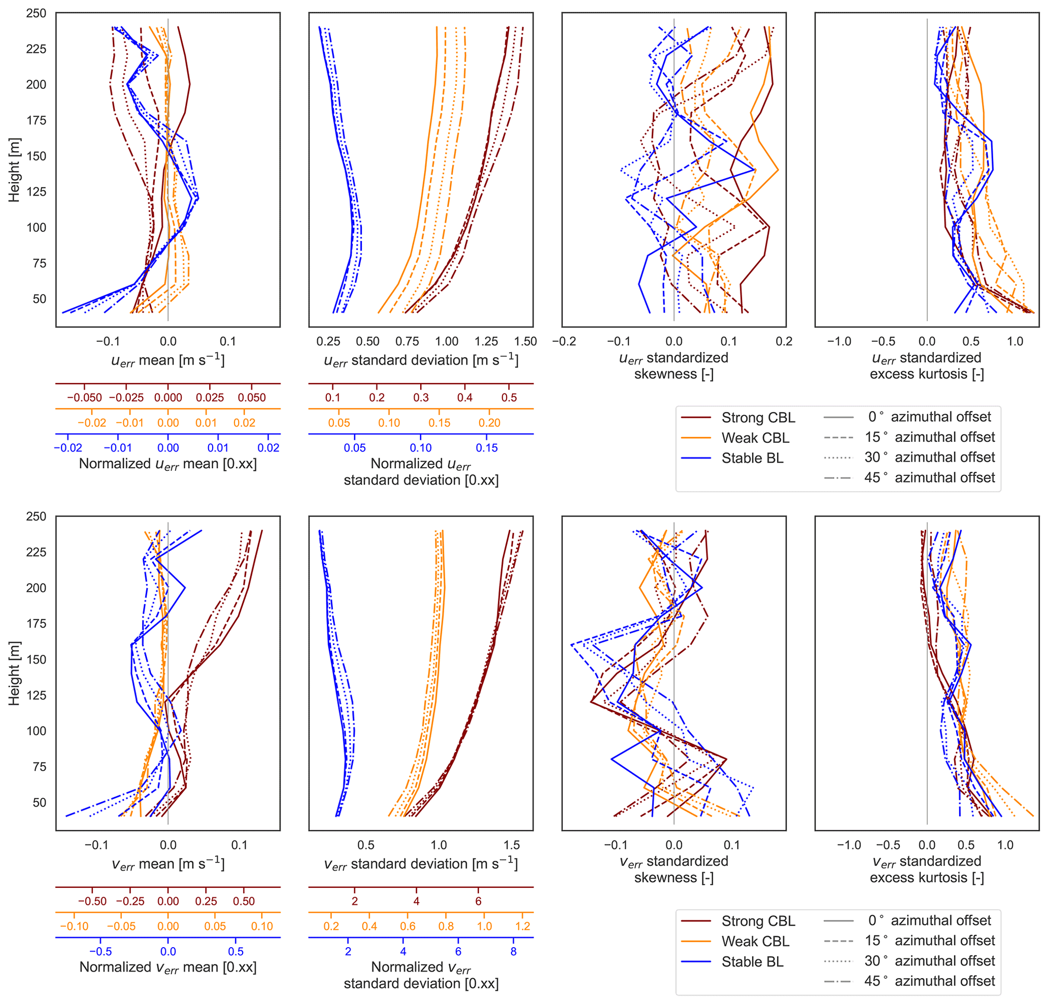
Figure A1 Comparison of u and v error distribution moments over disaggregated lidar orientation angles. No offset, same axes as LES domain (solid), rotated 15^∘ counterclockwise from LES domain axes (dashed), rotated 30^∘ counterclockwise (dotted), and rotated 45^∘ counterclockwise (dashed–dotted).

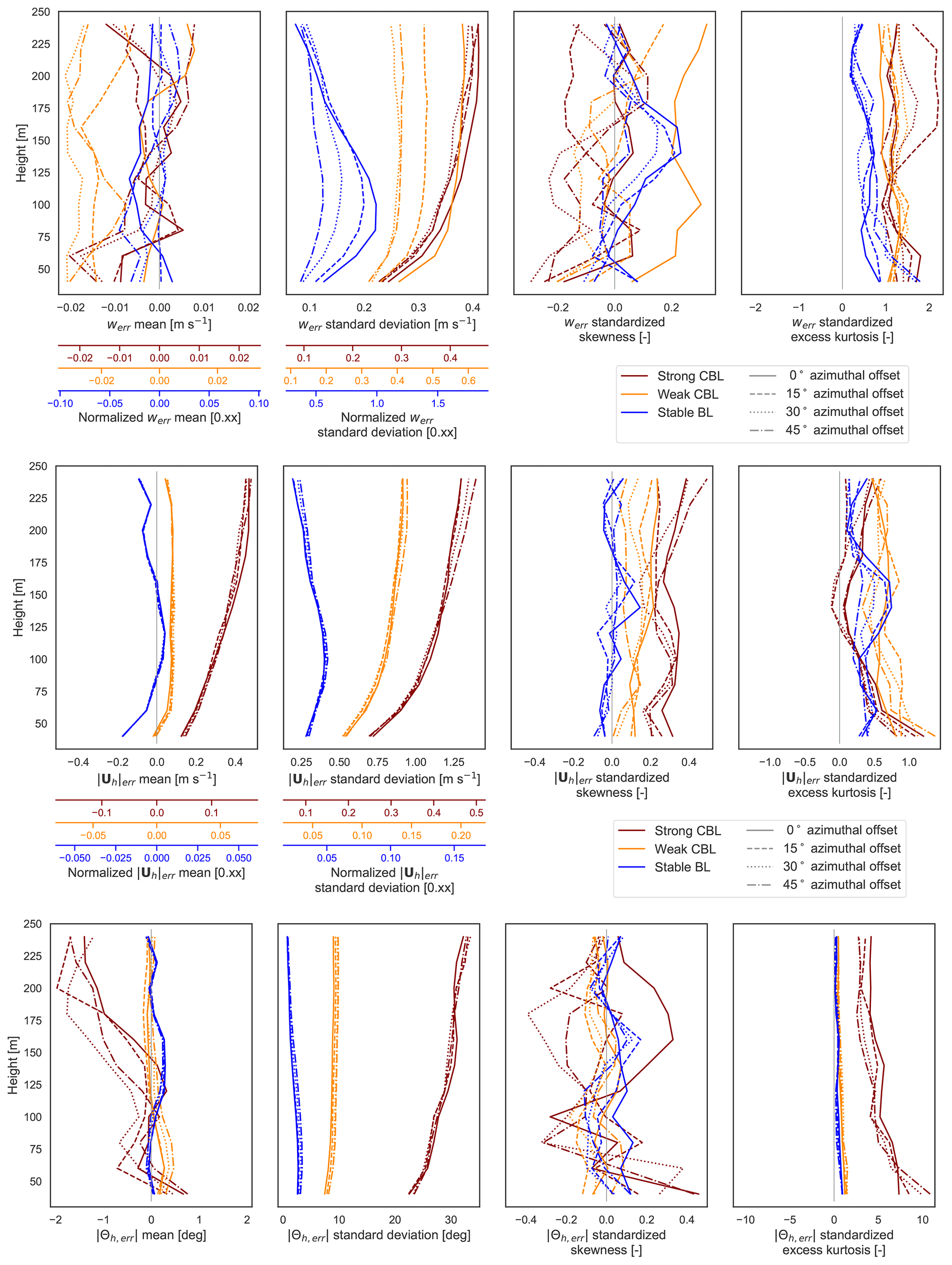
Figure A2 Comparison of error distribution moments over disaggregated lidar orientation angles. No offset, same axes as LES domain (solid), rotated 15^∘ counterclockwise from LES domain axes (dashed), rotated 30^∘ counterclockwise (dotted), and rotated 45^∘ counterclockwise (dashed–dotted).

Appendix B: Derivation of wind speed and direction error means

The mean wind speed error value is computed by taking the expected value of the random variable equation for wind speed error (Eq. 18). We can further simplify if the component errors are assumed to have a mean of zero.

$$\begin{array}{}\text{(B1)}& \begin{array}{rl}\mathit{\mu }\left(\right|{\mathit{U}}_h{|}_{\mathrm{err}})& =\mathit{\mu }\left[{\displaystyle \frac{U}{\left|{\mathit{U}}_h\right|}}{u}_{\mathrm{err}}+{\displaystyle \frac{V}{\left|{\mathit{U}}_h\right|}}{v}_{\mathrm{err}}+{\displaystyle \frac{u_{\mathrm{err}}^{\mathrm{2}}+v_{\mathrm{err}}^{\mathrm{2}}}{\mathrm{2}\left|{\mathit{U}}_h\right|}}\right]\\ & ={\displaystyle \frac{U}{\left|{\mathit{U}}_h\right|}}\mathit{\mu }\left(u_{\mathrm{err}}\right)+{\displaystyle \frac{V}{\left|{\mathit{U}}_h\right|}}\mathit{\mu }\left(v_{\mathrm{err}}\right)\\ & +{\displaystyle \frac{{\mathit{\sigma }}^{\mathrm{2}}\left(u_{\mathrm{err}}\right)+{\mathit{\mu }}^{\mathrm{2}}\left(u_{\mathrm{err}}\right)+{\mathit{\sigma }}^{\mathrm{2}}\left(v_{\mathrm{err}}\right)+{\mathit{\mu }}^{\mathrm{2}}\left(v_{\mathrm{err}}\right)}{\mathrm{2}\left|{\mathit{U}}_h\right|}}\\ & \approx {\displaystyle \frac{{\mathit{\sigma }}^{\mathrm{2}}\left(u_{\mathrm{err}}\right)+{\mathit{\sigma }}^{\mathrm{2}}\left(v_{\mathrm{err}}\right)}{\mathrm{2}\left|{\mathit{U}}_h\right|}}\end{array}\end{array}$$

The argument of the inverse tangent function in the wind direction error (Eq. 21) is the ratio of two random variables, each of which is a linear function of the component errors. We start by finding the expected value of the argument.

$$\begin{array}{}\text{(B2)}& {\displaystyle }\mathit{\mu }\left({\displaystyle \frac{V{u}_{\mathrm{err}}-U{v}_{\mathrm{err}}}{|{\mathit{U}}_h{|}^{\mathrm{2}}+U{u}_{\mathrm{err}}+V{v}_{\mathrm{err}}}}\right)=\mathit{\mu }\left({\displaystyle \frac{X}{Y}}\right)\end{array}$$

Using an established approximation for the expected value of a ratio of random variables based on Taylor series expansions (Kendall et al., 1994), we can expand the expected value of the ratio.

$$\begin{array}{}\text{(B3)}& {\displaystyle }\mathit{\mu }\left({\displaystyle \frac{X}{Y}}\right)\approx {\displaystyle \frac{\mathit{\mu }\left(X\right)}{\mathit{\mu }\left(Y\right)}}-{\displaystyle \frac{\text{Cov}(X,Y)}{\left[\mathit{\mu }\right(Y){]}^{\mathrm{2}}}}+{\displaystyle \frac{{\mathit{\sigma }}^{\mathrm{2}}\left(Y\right)\mathit{\mu }\left(X\right)}{\left[\mathit{\mu }\right(Y){]}^{\mathrm{3}}}}\end{array}$$

Letting X and Y refer to the numerator and denominator of the bound, respectively, we can solve for the means. If we assume the u and v component errors are zero, we may simplify further.

$$\begin{array}{}\text{(B4)}& \mathit{\mu }\left(X\right)=\mathit{\mu }(V{u}_{\mathrm{err}}-U{v}_{\mathrm{err}})=V\mathit{\mu }\left(u_{\mathrm{err}}\right)-U\mathit{\mu }\left(v_{\mathrm{err}}\right)\approx \mathrm{0}\end{array}$$

$$\begin{array}{}\text{(B5)}& \begin{array}{rl}\mathit{\mu }\left(Y\right)& =\mathit{\mu }\left(\right|{\mathit{U}}_h{|}^{\mathrm{2}}+U{u}_{\mathrm{err}}+V{v}_{\mathrm{err}})=|{\mathit{U}}_h{|}^{\mathrm{2}}\\ & +U\mathit{\mu }\left(u_{\mathrm{err}}\right)+V\mathit{\mu }\left(v_{\mathrm{err}}\right)\approx |{\mathit{U}}_h{|}^{\mathrm{2}}\end{array}\end{array}$$

Assuming u_err and v_err have zero mean, giving us the result for the means of X and Y above, and further that u_err and v_err are uncorrelated, we compute the covariance.

$$\begin{array}{rl}& \text{Cov}(X,Y)=\text{Cov}\left(V{u}_{\mathrm{err}}-U{v}_{\mathrm{err}},|{\mathit{U}}_h{|}^{\mathrm{2}}+U{u}_{\mathrm{err}}\right.\\ & \left.+V{v}_{\mathrm{err}}\right)=\mathit{\mu }\left[(V{u}_{\mathrm{err}}-U{v}_{\mathrm{err}})\left(|{\mathit{U}}_h{|}^{\mathrm{2}}+U{u}_{\mathrm{err}}\right.\right.\end{array}$$

$$\begin{array}{}\text{(B6)}& \begin{array}{rl}& \left.\left.+V{v}_{\mathrm{err}}-|{\mathit{U}}_h{|}^{\mathrm{2}}\right)\right]\\ & =\mathit{\mu }\left[UV{u}_{\mathrm{err}}^{\mathrm{2}}+V^{\mathrm{2}}{u}_{\mathrm{err}}{v}_{\mathrm{err}}-U^{\mathrm{2}}{u}_{\mathrm{err}}{v}_{\mathrm{err}}-UV{v}_{\mathrm{err}}^{\mathrm{2}}\right]\\ & \approx UV\left[{\mathit{\sigma }}^{\mathrm{2}}\left(u_{\mathrm{err}}\right)-{\mathit{\sigma }}^{\mathrm{2}}\left(v_{\mathrm{err}}\right)\right]\end{array}\end{array}$$

Similarly, we can obtain the variance with the same assumptions about the means of the u_err and v_err.

$$\begin{array}{ll}{\displaystyle }{\mathit{\sigma }}^{\mathrm{2}}\left(Y\right)& {\displaystyle }=\mathit{\mu }\left[\left(\right|{\mathit{U}}_h{|}^{\mathrm{2}}+U{u}_{\mathrm{err}}+V{v}_{\mathrm{err}}-|{\mathit{U}}_h{|}^{\mathrm{2}}{)}^{\mathrm{2}}\right]\\ \text{(B7)}& {\displaystyle }& {\displaystyle }=\mathit{\mu }\left[U^{\mathrm{2}}{u}_{\mathrm{err}}^{\mathrm{2}}-\mathrm{2}UV{u}_{\mathrm{err}}{v}_{\mathrm{err}}+V^{\mathrm{2}}{v}_{\mathrm{err}}^{\mathrm{2}}\right]\text{(B8)}& {\displaystyle }& {\displaystyle }\approx U^{\mathrm{2}}{\mathit{\sigma }}^{\mathrm{2}}\left(u_{\mathrm{err}}\right)+V^{\mathrm{2}}{\mathit{\sigma }}^{\mathrm{2}}\left(v_{\mathrm{err}}\right)\end{array}$$

Substituting back into Eq. (B3),

$$\begin{array}{}\text{(B9)}& \begin{array}{rl}\mathit{\mu }\left({\displaystyle \frac{X}{Y}}\right)& \approx {\displaystyle \frac{\mathrm{0}}{|{\mathit{U}}_h{|}^{\mathrm{2}}}}-{\displaystyle \frac{UV\left[{\mathit{\sigma }}^{\mathrm{2}}\left(u_{\mathrm{err}}\right)-{\mathit{\sigma }}^{\mathrm{2}}\left(v_{\mathrm{err}}\right)\right]}{|{\mathit{U}}_h{|}^{\mathrm{4}}}}\\ & +{\displaystyle \frac{\left[U^{\mathrm{2}}{\mathit{\sigma }}^{\mathrm{2}}\right(u_{\mathrm{err}})+V^{\mathrm{2}}{\mathit{\sigma }}^{\mathrm{2}}(v_{\mathrm{err}}\left)\right]\cdot \mathrm{0}}{|{\mathit{U}}_h{|}^{\mathrm{6}}}}\\ & =-{\displaystyle \frac{UV\left[{\mathit{\sigma }}^{\mathrm{2}}\left(u_{\mathrm{err}}\right)-{\mathit{\sigma }}^{\mathrm{2}}\left(v_{\mathrm{err}}\right)\right]}{|{\mathit{U}}_h{|}^{\mathrm{4}}}}\approx \mathrm{0}.\end{array}\end{array}$$

If the wind component errors have zero mean and are uncorrelated, then we get the expected bias in Eq. (B9). The remaining term should be small if the variance of u_err and v_err is similar and the wind speed is appreciable (making $|{\mathit{U}}_h{|}^{\mathrm{4}}$ large). The approximation of zero mean bias, lack of correlation, and similar variances holds when the horizontal error vector (u_err,v_err)^T has a direction about evenly distributed and the magnitude is relatively consistent about the circle.

Even in the presence of small biases in u and v, moderate winds serve to keep any bias in the wind direction in check. In the presence of very weak winds, however, small deviations of the mean biases from zero can be magnified in the wind direction bias.

The mean wind direction error is given by $\mathit{\mu }\left(\arctan \right(X/Y\left)\right)=\arctan \left(\mathit{\mu }\right(X/Y\left)\right)$. Since we expect the mean of the ratio to be close to zero, so too do we expect the wind direction bias to be close to zero.

Appendix C: Derivation of error bound on RWF-weighted radial velocity measurement

Let v_r(r₀) be the actual radial velocity at radius r₀ and ${\stackrel{\mathrm{‾}}{v}}_r\left(r_{\mathrm{0}}\right)$ the observed, range-gate-weighted radial velocity centered at r₀. Let R>0 be an arbitrary threshold to split the integral.

We will assume the v_r(s) profile has at least two continuous derivatives. The range-gate weighting function, ρ(s), should generally be non-negative and symmetric and satisfy ${\int }_{-\mathrm{\infty }}^{\mathrm{\infty }}\mathit{\rho }\left(s\right)\mathrm{d}s=\mathrm{1}$ by definition, so we assume these properties as well.

Using the triangle inequality, integral mean value theorem, and Taylor series expansion, we have the following derivation.

$$\begin{array}{}\text{(C1)}& \begin{array}{rl}& \left|{\stackrel{\mathrm{‾}}{v}}_r\left(r_{\mathrm{0}}\right)-v_{\mathrm{r}}\left(r_{\mathrm{0}}\right)\right|=\left|\underset{-\mathrm{\infty }}{\overset{\mathrm{\infty }}{\int }}\mathit{\rho }\left(s\right)v_{\mathrm{r}}(r_{\mathrm{0}}+s)\mathrm{d}s-v_{\mathrm{r}}\left(r_{\mathrm{0}}\right)\right|\\ & \le \left|\underset{\left|s\right|>R}{\int }\mathit{\rho }\left(s\right)v_{\mathrm{r}}(r_{\mathrm{0}}+s)\mathrm{d}s\right|\\ & +\left|\underset{\left|s\right|\le R}{\int }\mathit{\rho }\left(s\right)v_{\mathrm{r}}(r_{\mathrm{0}}+s)\mathrm{d}s-v_{\mathrm{r}}\left(r_{\mathrm{0}}\right)\right|\\ & \le \underset{\left|s\right|>R}{max}\left|v_{\mathrm{r}}\right(r_{\mathrm{0}}+s\left)\right|\underset{\left|s\right|>R}{\int }\mathit{\rho }\left(s\right)\mathrm{d}s\\ & +\left|\underset{\left|s\right|\le R}{\int }\mathit{\rho }\left(s\right)v_{\mathrm{r}}(r_{\mathrm{0}}+s)\mathrm{d}s-v_{\mathrm{r}}\left(r_{\mathrm{0}}\right)\right|\\ & =\underset{\left|s\right|>R}{max}\left|v_{\mathrm{r}}\right(r_{\mathrm{0}}+s\left)\right|\underset{\left|s\right|>R}{\int }\mathit{\rho }\left(s\right)\mathrm{d}s\\ & +\left|\underset{\left|s\right|\le R}{\int }\mathit{\rho }\left(s\right)\left[v_{\mathrm{r}}\left(r_{\mathrm{0}}\right)+v_{\mathrm{r}}^{\prime }\left(r_{\mathrm{0}}\right)s\right.\right.\\ & \left.\left.+{\displaystyle \frac{\mathrm{1}}{\mathrm{2}}}{v}_{\mathrm{r}}^{\prime \prime }(r_{\mathrm{0}}+\mathit{\xi }(s\left)\right)s^{\mathrm{2}}\right]\mathrm{d}s-v_{\mathrm{r}}\left(r_{\mathrm{0}}\right)\right|\\ & =\underset{\left|s\right|>R}{max}\left|v_{\mathrm{r}}\right(r_{\mathrm{0}}+s\left)\right|\left[\mathrm{1}-\underset{\left|s\right|\le R}{\int }\mathit{\rho }\left(s\right)\mathrm{d}s\right]\\ & +\left|v_{\mathrm{r}}\left(r_{\mathrm{0}}\right)\left(\underset{\left|s\right|\le R}{\int }\mathit{\rho }\left(s\right)\mathrm{d}s-\mathrm{1}\right)\right.\\ & \left.+v_{\mathrm{r}}^{\prime }\left(r_{\mathrm{0}}\right)\underset{\left|s\right|\le R}{\int }\mathit{\rho }\left(s\right)s\mathrm{d}s+{\displaystyle \frac{\mathrm{1}}{\mathrm{2}}}{v}_{\mathrm{r}}^{\prime \prime }(r_{\mathrm{0}}+{\mathit{\xi }}_{*})\underset{\left|s\right|\le R}{\int }\mathit{\rho }\left(s\right)s^{\mathrm{2}}\mathrm{d}s\right|\\ & \le \left[\mathrm{1}-\underset{\left|s\right|\le R}{\int }\mathit{\rho }\left(s\right)\mathrm{d}s\right]\left(\underset{\left|s\right|>R}{max}\left|v_{\mathrm{r}}\right(r_{\mathrm{0}}+s\left)\right|\right.\\ & \left.+\left|v_{\mathrm{r}}\right(r_{\mathrm{0}}\left)\right|\right)+\left[{\displaystyle \frac{\mathrm{1}}{\mathrm{2}}}\underset{\left|s\right|\le R}{\int }\mathit{\rho }\left(s\right)s^{\mathrm{2}}\mathrm{d}s\right]\left|v_{\mathrm{r}}^{\prime \prime }\right(r_{\mathrm{0}}+{\mathit{\xi }}_{*}\left)\right|\end{array}\end{array}$$

Where we have introduced $\mathit{\xi }:[-R,R]\to [-R,R]$ as part of the Taylor remainder. The relative sizes of the coefficients with choice of R in the WindCube V2 RWF (Eq. 6) are plotted in Fig. C1.

Figure C1 Growth and decay of the coefficients in the bounding terms of the radial velocity measurement error with increasing threshold distance, R. The WindCube V2 RWF (Eq. 6 with parameters in Table 1) is used for illustration.

Appendix D: Numeric computation of RWF convolution

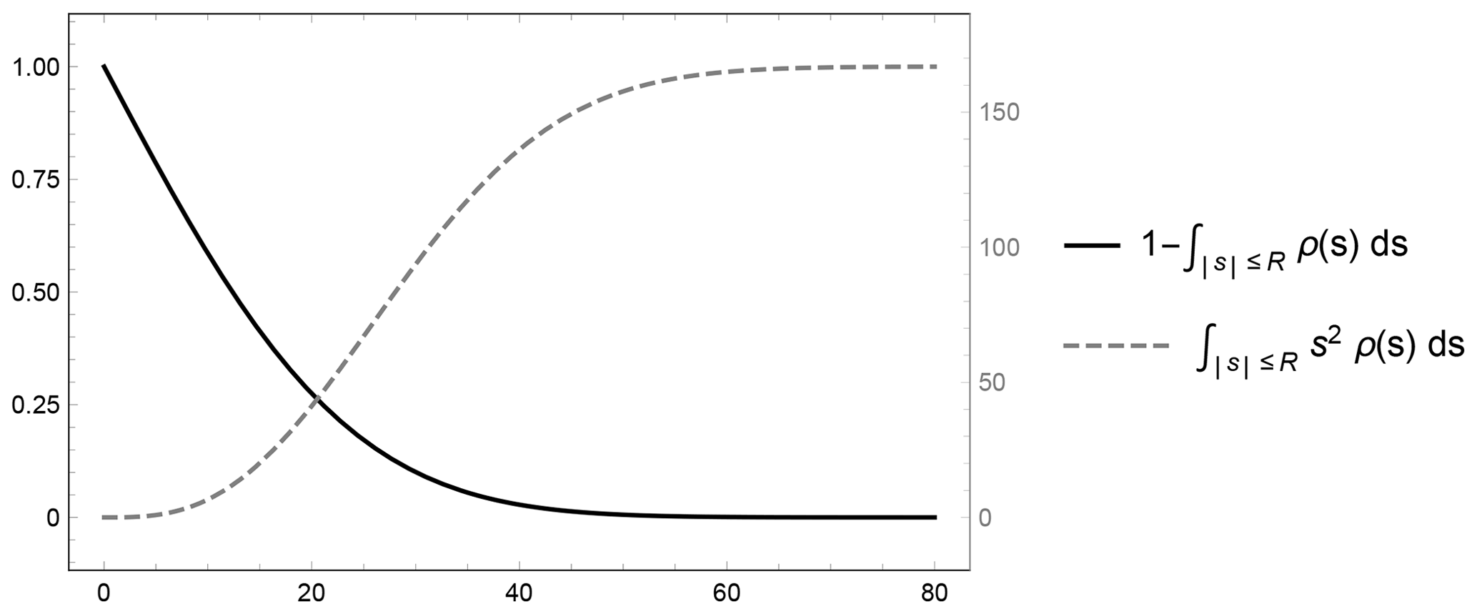
The numeric computation of the range-gate-weighted radial velocity involves approximating a convolution integral for a continuous weighted average. The estimate should ideally maintain the weighted average nature of the operation to prevent under-estimating the result by virtue of only incorporating a sub-unity set of weights. For this reason, previous implementations (Forsting et al., 2017; Lundquist et al., 2015) have implemented the RWF convolution as a discrete weighted average using re-normalized RWF values at the corresponding points.

$$\begin{array}{}\text{(D1)}& \begin{array}{rl}& \underset{-\mathrm{\infty }}{\overset{\mathrm{\infty }}{\int }}\mathit{\rho }\left(s\right)v_{\mathrm{r}}(r+s)\mathrm{d}s\approx \underset{-R}{\overset{R}{\int }}\mathit{\rho }\left(s\right)v_{\mathrm{r}}(r+s)\mathrm{d}s\\ & \approx {\displaystyle \frac{\mathrm{1}}{{\sum }_i\mathit{\rho }\left(s_i\right)}}\sum _k\mathit{\rho }\left(s_k\right)v_{\mathrm{r}}\left(s_k\right)\end{array}\end{array}$$

The quadrature form amounts to a re-scaled midpoint rule when the nodes ({s_k}) are equispaced; rewrite to show explicitly re-normalized RWF values at the corresponding points.

$$\begin{array}{}\text{(D2)}& \begin{array}{rl}& \sum _k{\displaystyle \frac{\mathit{\rho }\left(s_k\right)}{{\sum }_i\mathit{\rho }\left(s_i\right)}}{v}_{\mathrm{r}}\left(s_k\right)=\sum _k{\displaystyle \frac{h\mathit{\rho }\left(s_k\right)}{h{\sum }_i\mathit{\rho }\left(s_i\right)}}{v}_{\mathrm{r}}\left(s_k\right)\\ & ={\displaystyle \frac{\mathrm{1}}{{\sum }_{i}h\mathit{\rho }\left(s_i\right)}}\sum _{k}h\mathit{\rho }\left(s_k\right)v_{\mathrm{r}}\left(s_k\right)\end{array}\end{array}$$

For nodes that are not equispaced, it suggests that the variable interval width, h_k, should be incorporated into the approximation such that it is still a re-scaled mid-point rule.

$$\begin{array}{}\text{(D3)}& {\displaystyle }\underset{-\mathrm{\infty }}{\overset{\mathrm{\infty }}{\int }}\mathit{\rho }\left(s\right)v_{\mathrm{r}}(r+s)\mathrm{d}s\approx {\displaystyle \frac{\mathrm{1}}{{\sum }_i{h}_i\mathit{\rho }\left(s_i\right)}}\sum _k{h}_k\mathit{\rho }\left(s_k\right)v_{\mathrm{r}}\left(s_k\right)\end{array}$$

First, we will truncate the domain over which we try to estimate the integral to a finite interval. The omitted contribution from the ends of the infinite integration interval can be bound small using the fact that the tails of the RWF must vanish in order for the infinite integral ${\int }_{-\mathrm{\infty }}^{\mathrm{\infty }}\mathit{\rho }\left(s\right)\mathrm{d}s=\mathrm{1}$ to converge.

$$\begin{array}{}\text{(D4)}& \begin{array}{rl}& \left|{\displaystyle \frac{\mathrm{1}}{{\sum }_i{h}_i\mathit{\rho }\left(s_i\right)}}\sum _k{h}_k\mathit{\rho }\left(s_k\right)v_{\mathrm{r}}(r+s_k)-\underset{-\mathrm{\infty }}{\overset{\mathrm{\infty }}{\int }}\mathit{\rho }\left(s\right)v_{\mathrm{r}}(r+s)\mathrm{d}s\right|\\ \le & \left|{\displaystyle \frac{\mathrm{1}}{{\sum }_i{h}_i\mathit{\rho }\left(s_i\right)}}\sum _k{h}_k\mathit{\rho }\left(s_k\right)v_{\mathrm{r}}(r+s_k)-\underset{-R}{\overset{R}{\int }}\mathit{\rho }\left(s\right)v_{\mathrm{r}}(r+s)\mathrm{d}s\right|\\ & +\left|\underset{\left|s\right|>R}{\int }\mathit{\rho }\left(s\right)v_{\mathrm{r}}(r+s)\mathrm{d}s\right|\\ \le & \left|{\displaystyle \frac{\mathrm{1}}{{\sum }_i{h}_i\mathit{\rho }\left(s_i\right)}}\sum _k{h}_k\mathit{\rho }\left(s_k\right)v_{\mathrm{r}}(r+s_k)-\underset{-R}{\overset{R}{\int }}\mathit{\rho }\left(s\right)v_{\mathrm{r}}(r+s)\mathrm{d}s\right|\\ & +\left[\underset{\left|s\right|>R}{\int }\mathit{\rho }\left(s\right)\mathrm{d}s\right]\underset{\left|s\right|>R}{max}\left|v\right(r+s\left)\right|\end{array}\end{array}$$

The error bound on the numeric quadrature will be derived based on the mid-point rule. Consider just one sub-interval of length h_k with the mid-point at s_k.

$$\begin{array}{rl}& \left|{\displaystyle \frac{\mathrm{1}}{{\sum }_i{h}_i\mathit{\rho }\left(s_i\right)}}{h}_k\mathit{\rho }\left(s_k\right)v_{\mathrm{r}}(r+s_k)-\underset{s_k-h_k/\mathrm{2}}{\overset{s_k+h_k/\mathrm{2}}{\int }}\mathit{\rho }\left(s\right)v_{\mathrm{r}}(r+s)\mathrm{d}s\right|\\ =& \left|{\displaystyle \frac{\mathrm{1}}{{\sum }_i{h}_i\mathit{\rho }\left(s_i\right)}}{h}_k\mathit{\rho }\left(s_k\right)v_{\mathrm{r}}(r+s_k)-\underset{s_k-h_k/\mathrm{2}}{\overset{s_k+h_k/\mathrm{2}}{\int }}\right.\\ & \left[\mathit{\rho }\left(s_k\right)v_{\mathrm{r}}(r+s_k)+{\left(\mathit{\rho }\left(s_k\right)v_{\mathrm{r}}(r+s_k)\right)}^{\prime }(s-s_k)\right.\\ & \left.\left.+{\displaystyle \frac{\mathrm{1}}{\mathrm{2}}}{\left(\mathit{\rho }\left({\mathit{\xi }}_k\right)v_{\mathrm{r}}(r+{\mathit{\xi }}_k(s\left)\right)\right)}^{\prime \prime }(s-s_k{)}^{\mathrm{2}}\right]\mathrm{d}s\right|\end{array}$$

$$\begin{array}{}\text{(D5)}& \begin{array}{rl}=& \left|{\displaystyle \frac{\mathrm{1}}{{\sum }_i{h}_i\mathit{\rho }\left(s_i\right)}}{h}_k\mathit{\rho }\left(s_k\right)v_{\mathrm{r}}(r+s_k)\right.\\ & -\underset{s_k-h_k/\mathrm{2}}{\overset{s_k+h_k/\mathrm{2}}{\int }}\left[\mathit{\rho }\left(s_k\right)v_{\mathrm{r}}(r+s_k)\right.\\ & \left.\left.+{\displaystyle \frac{\mathrm{1}}{\mathrm{2}}}{\left(\mathit{\rho }\left({\mathit{\xi }}_k\right)v_{\mathrm{r}}(r+{\mathit{\xi }}_k(s\left)\right)\right)}^{\prime \prime }(s-s_k{)}^{\mathrm{2}}\right]\mathrm{d}s\right|\\ =& \left|{\displaystyle \frac{\mathrm{1}}{{\sum }_i{h}_i\mathit{\rho }\left(s_i\right)}}{h}_k\mathit{\rho }\left(s_k\right)v_{\mathrm{r}}(r+s_k)\right.\\ & -\mathit{\rho }\left(s_k\right)v_{\mathrm{r}}(r+s_k)h_k-{\displaystyle \frac{\mathrm{1}}{\mathrm{2}}}\\ & \left.\underset{s_k-h_k/\mathrm{2}}{\overset{s_k+h_k/\mathrm{2}}{\int }}{\left(\mathit{\rho }\left({\mathit{\xi }}_k\right)v_{\mathrm{r}}(r+{\mathit{\xi }}_k(s\left)\right)\right)}^{\prime \prime }(s-s_k{)}^{\mathrm{2}}\mathrm{d}s\right|\\ \le & \left|\left({\displaystyle \frac{\mathrm{1}}{{\sum }_i{h}_i\mathit{\rho }\left(s_i\right)}}-\mathrm{1}\right)h_k\mathit{\rho }\left(s_k\right)v_{\mathrm{r}}(r+s_k)\right|\\ & +\left|{\displaystyle \frac{\mathrm{1}}{\mathrm{2}}}\underset{s_k-h_k/\mathrm{2}}{\overset{s_k+h_k/\mathrm{2}}{\int }}{\left(\mathit{\rho }\left({\mathit{\xi }}_k\right)v_{\mathrm{r}}(r+{\mathit{\xi }}_k(s\left)\right)\right)}^{\prime \prime }{s}^{\mathrm{2}}\mathrm{d}s\right|\\ \le & \left|\left({\displaystyle \frac{\mathrm{1}}{{\sum }_i{h}_i\mathit{\rho }\left(s_i\right)}}-\mathrm{1}\right)h_k\mathit{\rho }\left(s_k\right)v_{\mathrm{r}}(r+s_k)\right|\\ & +{\displaystyle \frac{h_k^{\mathrm{3}}}{\mathrm{24}}}\underset{|{\mathit{\xi }}_k^{*}-s_k|\le h_k}{max}\left|{\left(\mathit{\rho }\left({\mathit{\xi }}_k\right)v_{\mathrm{r}}(r+{\mathit{\xi }}_k^{*})\right)}^{\prime \prime }\right|\end{array}\end{array}$$

Sum the error accumulated over all the intervals. If the sub-intervals partition the full interval $[-T,T]$, then

$$\begin{array}{}\text{(D6)}& \begin{array}{rl}& \left|{\displaystyle \frac{\mathrm{1}}{{\sum }_{i}h\mathit{\rho }\left(s_i\right)}}\sum _{k}h\mathit{\rho }\left(s_k\right)v_{\mathrm{r}}(r+s_k)-\underset{-T}{\overset{T}{\int }}\mathit{\rho }\left(s\right)v_{\mathrm{r}}(r+s)\mathrm{d}s\right|\\ \le & \sum _k\left|{\displaystyle \frac{\mathrm{1}}{{\sum }_{i}h\mathit{\rho }\left(s_i\right)}}{h}_k\mathit{\rho }\left(s_k\right)v_{\mathrm{r}}(r+s_k)\right.\\ & \left.-\underset{s_k-h_k/\mathrm{2}}{\overset{s_k+h_k/\mathrm{2}}{\int }}\mathit{\rho }\left(s\right)v_{\mathrm{r}}(r+s)\mathrm{d}s\right|\\ \le & \sum _k\left[\left|\left({\displaystyle \frac{\mathrm{1}}{{\sum }_i{h}_i\mathit{\rho }\left(s_i\right)}}-\mathrm{1}\right)h_k\mathit{\rho }\left(s_k\right)v_{\mathrm{r}}(r+s_k)\right|\right.\\ & \left.+{\displaystyle \frac{h_k^{\mathrm{3}}}{\mathrm{24}}}\underset{|{\mathit{\xi }}_k-s_k|\le h_k}{max}\left|{\left(\mathit{\rho }\left({\mathit{\xi }}_k\right)v_{\mathrm{r}}(r+{\mathit{\xi }}_k)\right)}^{\prime \prime }\right|\right]\\ \le & \left|{\displaystyle \frac{\mathrm{1}}{{\sum }_i{h}_i\mathit{\rho }\left(s_i\right)}}-\mathrm{1}\right|\sum _k{h}_k\mathit{\rho }\left(s_k\right)\left|v_{\mathrm{r}}(r+s_k)\right|\\ & +{\displaystyle \frac{{\sum }_k{h}_k^{\mathrm{3}}}{\mathrm{24}}}\underset{\left|\mathit{\xi }\right|\le R}{max}\left|{\left(\mathit{\rho }\left(\mathit{\xi }\right)v_{\mathrm{r}}(r+\mathit{\xi })\right)}^{\prime \prime }\right|\\ \le & \left|{\displaystyle \frac{\mathrm{1}}{{\sum }_i{h}_i\mathit{\rho }\left(s_i\right)}}-\mathrm{1}\right|\underset{k}{max}\left|v_{\mathrm{r}}(r+s_k)\right|\sum _k{h}_k\mathit{\rho }\left(s_k\right)\\ & +{\displaystyle \frac{{\sum }_k{h}_k^{\mathrm{3}}}{\mathrm{24}}}\underset{\left|\mathit{\xi }\right|\le R}{max}\left|{\left(\mathit{\rho }\left(\mathit{\xi }\right)v_{\mathrm{r}}(r+\mathit{\xi })\right)}^{\prime \prime }\right|\\ \le & \left|\mathrm{1}-\sum _k{h}_k\mathit{\rho }\left(s_k\right)\right|\underset{k}{max}\left|v_{\mathrm{r}}(r+s_k)\right|\\ & +{\displaystyle \frac{{\sum }_k{h}_k^{\mathrm{3}}}{\mathrm{24}}}\underset{\left|\mathit{\xi }\right|\le R}{max}\left|{\left(\mathit{\rho }\left(\mathit{\xi }\right)v_{\mathrm{r}}(r+\mathit{\xi })\right)}^{\prime \prime }\right|.\end{array}\end{array}$$

All together, the error of the numeric approximation of the integral may be bounded by

$$\begin{array}{}\text{(D7)}& \begin{array}{rl}& \left|{\displaystyle \frac{{\sum }_k{h}_k\mathit{\rho }\left(s_k\right)v_{\mathrm{r}}(r+s_k)}{{\sum }_i{h}_i\mathit{\rho }\left(s_i\right)}}-\underset{-\mathrm{\infty }}{\overset{\mathrm{\infty }}{\int }}\mathit{\rho }\left(s\right)v_{\mathrm{r}}(r+s)\mathrm{d}s\right|\\ & \le \left|\mathrm{1}-\sum _k{h}_k\mathit{\rho }\left(s_k\right)\right|\underset{k}{max}\left|v_{\mathrm{r}}(r+s_k)\right|+{\displaystyle \frac{{\sum }_k{h}_k^{\mathrm{3}}}{\mathrm{24}}}\\ & \underset{\left|\mathit{\xi }\right|\le R}{max}\left|{\left(\mathit{\rho }\left(\mathit{\xi }\right)v_{\mathrm{r}}(r+\mathit{\xi })\right)}^{\prime \prime }\right|\\ & +\left[\underset{\left|s\right|>R}{\int }\mathit{\rho }\left(s\right)\mathrm{d}s\right]\underset{\left|s\right|>R}{max}\left|v\right(r+s\left)\right|.\end{array}\end{array}$$

In addition to picking the interval $[-R,R]$ large enough so that the contribution from the tails is small and the usual second-order error term from the mid-point rule, the points should be selected so that the mid-point approximation of the integral of the RWF (i.e the first term) is close to 1.

Choices for nodes include (1) equispaced, (2) exponentially spaced, (3) equal RWF area, and (4) equal mid-point area h_kρ(s_k). Equispaced points are easy to determine and implement but do not maximize the utility of each point included. For a virtual lidar, which has to interpolate the winds for every node, inefficiently using points can be computationally expensive before the quadrature is even computed. The idea behind the other node distributions is to sample more heavily near the RWF center, where each point has greater impact on the result so that we reduce the number of low-utility nodes.

Exponentially spaced nodes (e.g. $\mathit{\{}-\mathrm{16},-\mathrm{8},-\mathrm{4},-\mathrm{2},-\mathrm{1},\mathrm{0},\mathrm{1},\mathrm{2},\mathrm{4},\mathrm{16}\mathit{\}}$) are easy to compute independently of the particular RWF function like the equispaced nodes, but crudely achieve the goal of clustering points more heavily close to the RWF center. Forsting et al. (2017) recommend using nodes spaced so that the integral of the RWF between nodes is constant. The result is nodes clustered more heavily toward the center and more equal weighting on each node (not over-sampling the tails). Based on the mid-point form and error bound derived earlier, we propose an alternative in the same vein. We can explicitly set the h_kρ(s_k) to be constant so that every point has equal weight. Starting with s₀=0 and $h_{\mathrm{0}}=\frac{\mathrm{1}}{N}$, where N is the total (odd) number of points, we can iteratively solve out for the symmetric nodes. In practice, the last nodes usually do not seem to be able to attain the same $h_k\mathit{\rho }\left(s_k\right)=\mathrm{1}/N$ weighting. Either the sum ∑_kh_kρ(s_k) must be reduced to less than 1 or the constant weighting relaxed for the end nodes. The latter is preferable to reduce the overall error.

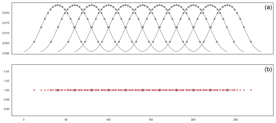
Figure D1 Using 15 points per range gate, the node locations {s_k} found by imposing h_kρ(s_k) to be constant for the WindCube V2 RWF for as many nodes as possible. The top panel shows node locations on the overlapping RWF centered at each of the 11 range gates. The bottom panel shows the nodes (x^′s) and range-gate centers (dots) along the one-dimensional beam length.

Selecting nodes for computational expediency in the case of multiple range gates along a beam introduces further considerations than those for a single range gate. For the WindCube V2, the intervals of dependency for the 20 m spaced range gates overlap (Fig. D1); nodes should be reused where possible rather than interpolating a separate set of points for each range gate. Methods using spacing according to the RWF area or imposing constant weighting are likely to produce unusual numbers that do not necessarily coincide between multiple range gates. Exponential spacing makes it easier to impose overlap in position. The cluster of points at the center of one range gate appear at the tail of another range gate and would have to be sub-selected to the desired points.