Balloon-borne aerosol–cloud interaction studies (BACIS): field campaigns to understand and quantify aerosol effects on clouds

A better understanding of aerosol–cloud interaction processes is important to quantify the role of clouds and aerosols on the climate system. There have been significant efforts to explain the ways aerosols modulate cloud properties. However, from the observational point of view, it is indeed challenging to observe and/or verify some of these processes because no single instrument or platform has been proven to be sufficient. Discrimination between aerosol and cloud is vital for the quantification of aerosol–cloud interaction. With this motivation, a set of observational field campaigns named balloon-borne aerosol–cloud interaction studies (BACIS) is proposed and conducted using balloon-borne in situ measurements in addition to the ground-based (lidar; mesosphere, stratosphere and troposphere (MST) radar; lower atmospheric wind profiler; microwave radiometer; ceilometer) and space-borne (CALIPSO) remote sensing instruments from Gadanki (13.45^∘ N, 79.2^∘ E), India. So far, 15 campaigns have been conducted as a part of BACIS campaigns from 2017 to 2020. This paper presents the concept of the observational approach, lists the major objectives of the campaigns, describes the instruments deployed, and discusses results from selected campaigns. Balloon-borne measurements of aerosol and cloud backscatter ratio and cloud particle count are qualitatively assessed using the range-corrected data from simultaneous observations of ground-based and space-borne lidars. Aerosol and cloud vertical profiles obtained in multi-instrumental observations are found to reasonably agree. Apart from this, balloon-borne profiling is found to provide information on clouds missed by ground-based and/or space-borne lidar. A combination of the Compact Optical Backscatter AerosoL Detector (COBALD) and Cloud Particle Sensor (CPS) sonde is employed for the first time in this study to discriminate cloud and aerosol in an in situ profile. A threshold value of the COBALD colour index (CI) for ice clouds is found to be between 18 and 20, and CI values for coarse-mode aerosol particles range between 11 and 15. Using the data from balloon measurements, the relationship between cloud and aerosol is quantified for the liquid clouds. A statistically significant slope (aerosol–cloud interaction index) of 0.77 found between aerosol backscatter and cloud particle count reveals the role of aerosol in the cloud activation process. In a nutshell, the results presented here demonstrate the observational approach to quantifying aerosol–cloud interactions.

1 Introduction

Understanding the fundamental process of aerosol–cloud interactions has been challenging issue in the scientific community for more than 3 decades (Seinfeld et al., 2016). The first ever observational evidence from analysis of ship tracks using satellite imagery opened up a wide scope for further research in this area (Coakley et al., 1987; Radke et al., 1989). Since then, efforts have been undertaken using different observational and modelling techniques and have led to a significant development in process-based understanding, quantification, and modelling of these interactions (Abbott and Cronin, 2021; Fan et al., 2018; Haywood and Boucher, 2000; Koren et al., 2010; Lohmann, 2006; Lohmann and Feichter, 2005; Rosenfeld et al., 2008, 2014b). Despite all of these efforts, radiative forcing estimates of both cloud modification and further adjustments (ERFaci) still show large uncertainties (IPCC, 2021) in the range −0.3 to −1.7 W m⁻² due to aerosol–cloud interactions. Apart from this, climate model simulations have uncertainties because parameterization schemes are inefficient in representing the ways that aerosols interact with clouds (Fan et al., 2016; Rosenfeld et al., 2014b; Seinfeld et al., 2016). At the process level, various hypotheses have been proposed since the first indirect effects were observed almost 4 decades ago (Twomey, 1977). All aerosol–cloud effects are found to act in a specific way for each cloud type, background meteorology, and dynamical condition. For example, the invigoration effect is proposed for convective clouds (Rosenfeld et al., 2014a) under the influence of updraughts. The first indirect effect (Twomey effect) and the second indirect effect (Albrecht effect) for liquid clouds are influenced by mixing (Costantino and Bréon, 2010), turbulence, and entrainment (Jose et al., 2020; Schmidt et al., 2015; Small et al., 2009). Although the first indirect effect is reasonably well understood, observational limitations pose a serious challenge in understanding and/or evaluating other hypotheses.

Among the various observational techniques that are currently available (ground-based, space-borne remote sensing, and aircraft or uncrewed aerial vehicles; UAV), none of the techniques alone has been proven to be self-sufficient in aerosol–cloud interaction studies. For example, ground-based (and/or space-borne) lidars suffer serious attenuation and even losses of observations due to the presence of optically thick cloud layers in the atmosphere. Thus, they may not be able to represent the complete vertical structure of clouds and aerosols. Note that information on aerosol and cloud profiles is essential for the estimation of their climate effects. Similarly, satellite data sets have shown distinct results and conclusions (Grosvenor et al., 2018; Koren et al., 2010; McComiskey and Feingold, 2012) using different analytical methods, e.g. changing grid resolutions. In addition, in situ measurements using aircraft and UAVs have been remarkable for obtaining detailed information on the microphysics of cloud and aerosol (Corrigan et al., 2008; Girdwood et al., 2020, 2022; Kulkarni et al., 2012; Mamali et al., 2018; Redemann et al., 2021; Weinzierl et al., 2017). However, there are serious limitations concerning altitude coverage, the feasibility of conducting aircraft or UAV campaigns, and the overall cost involved. There is also a chance that the aircraft perturbs the atmosphere before it measures cloud and aerosol data. Therefore, it is essential to examine the combined information on aerosols, clouds, and environmental parameters obtained simultaneously using multi-instrumental techniques.

A classic paper by Feingold et al. (2003) quantified the “Twomey effect” for the first time using ground-based remote sensing instruments such as a microwave radiometer (MWR), cloud radar, and a Raman lidar. In an intensive operations programme, Feingold et al. (2006) conducted airborne in situ measurements for obtaining the cloud effective radius using an aircraft in addition to the ground-based and space-borne remote sensing instruments. Pandithurai et al. (2009) also quantified the “Twomey effect” using a suite of ground-based remote sensing instruments (cloud radar, MWR, polarization lidar) and surface aerosol measurements (aerosol size distribution, scattering coefficient, and cloud condensation nuclei concentration). Similarly, Sena et al. (2016) utilized 14 years of coincident observations from cloud radar and a ceilometer, along with surface-reaching shortwave radiation measurements from the Atmospheric Radiation Measurement (ARM) program over the southern Great Plains in the USA, to investigate aerosol modifications of cloud macroscopic parameters and radiative properties rather than cloud microphysical parameters. In addition to simultaneous measurements of cloud and aerosol, concurrent measurements of thermodynamic and dynamic parameters of the atmosphere are also needed to thoroughly understand the process of aerosol–cloud interactions. As a step forward in this direction, McComiskey et al. (2009) used long-term, statistically robust ground-based remote sensing data from Point Reyes, California, to not only quantify the “Twomey effect” but also examine the factors influencing the variability in aerosol indirect effects such as updraught velocity, liquid water path, scale, and the resolution of observations. Using a novel dual-field-of-view Raman lidar and Doppler lidar technique, Schmidt et al. (2014) analysed the data from Leipzig, Germany, to explore linkages between aerosol, cloud properties, and the influence of updraughts. Sarna and Russchenberg (2016) used synergized measurements from a lidar (ceilometer), radar (cloud radar), and a radiometer (MWR) collected at ARM Mobile facility at Graciosa, the Azores, Portugal, and the Cabauw Experimental Site for Atmospheric Research (CESAR) observatory, The Netherlands, to not only quantify the aerosol indirect effect but also to attempt to disentangle the effects of vertical wind (Sarna and Russchenberg, 2017). All of these studies contributed significantly to our knowledge of aerosol–cloud interactions but are based on remote sensing techniques and limited to low-level, warm, and non-precipitating clouds.

Given the measurement limitations discussed above in ground-based multi-instrumental techniques, a balloon-borne in situ measurement is suggested to be the complementary technique as balloons can pass through the cloud (during their ascent and descent), representing the vertical structure of the cloud and aerosol below and above the cloud near simultaneously (see Sect. 2 for details) without perturbing the atmosphere. Although there is less information and data regarding balloon-based aerosol sampling artefacts than for conventional aircraft, information from balloon-borne in situ measurements in combination with the ground-based and/or space-borne remote sensing instruments will be of great help in constructing the complete vertical profiles of aerosol and cloud and further understanding the process of aerosol–cloud interactions. With this in mind, a balloon-borne field campaign named BACIS (Balloon-borne Aerosol Cloud Interaction Studies) was initiated in the year 2017 at the National Atmospheric Research Laboratory (NARL) in Gadanki (13.45^∘ N, 79.2^∘ E), India, with the multi-instrumental approach.

Balloon-borne measurements of aerosol and cloud were first reported in Rosen and Kjome (1991) using a self-developed backscatter sonde. The Compact Optical Backscatter AerosoL Detector (COBALD) is similar to this device but is classified as a lightweight sonde (Brabec et al., 2012). Measurements of aerosol size distribution in the stratosphere were carried out using an optical particle counter developed at the University of Wyoming (Deshler et al., 2003). Smith et al. (2019) developed a novel, low-cost, and lightweight open-path configuration optical particle counter, UCASS (Universal Cloud Aerosol Sampling System), for a wide range of particle size measurements covering both aerosol and cloud. Kezoudi et al. (2021) and Mamali et al. (2018) used UCASS to report balloon-borne in situ measurements of dust aerosol and compared UCASS with ground-based and airborne instruments. However, BACIS campaigns are designed to understand and quantify aerosol–cloud interactions. For this, a combination of balloon-borne sondes, COBALD, and a cloud particle sensor (CPS) is used for the first time to separate and discriminate aerosol and cloud in a profile. Note that COBALD and CPS have been used individually in other studies (Brunamonti et al., 2018, 2021; Fujiwara et al., 2016; Hanumanthu et al., 2020; Inoue et al., 2021; Vernier et al., 2015, 2018).

The purpose of this paper is to introduce the motivation and objectives of the BACIS campaigns for quantifying aerosol–cloud interactions. In order to do this, we have discussed most of the related topics, such as the campaign approach, sensors and instruments employed, and analytical methods, and have compared the balloon features. Results from selected campaigns focus on the discrimination of aerosol and cloud in a profile. Overall, the methods presented in this paper for the data analysis and processing are novel. Using these methods, aerosol–cloud interaction is estimated in liquid clouds.

2 Instruments and methods

2.1 Balloon-borne sensors

2.1.1 COBALD

The Compact Optical Backscatter AerosoL Detector (COBALD) deployed in BACIS campaigns is a lightweight (540 g) balloon-borne sonde developed in the group of Thomas Peter at ETH Zurich, Switzerland. It is essentially a miniaturized version of the backscatter sonde developed by Rosen and Kjome (1991). A backscatter sonde is a balloon-borne sensor that measures the backscattered light from molecules, aerosol, and clouds at two wavelengths in the vicinity of the sonde as it passes through the atmospheric column. COBALD consists of two LED light sources of approximately 500 mW power emitting at 455 nm (blue) and 940 nm (termed “infrared”) wavelengths, respectively (Brabec et al., 2012). The light emitted by the sonde illuminates the air in the vicinity, and backscattered light from an ensemble of particles is detected using a silicon photodetector. The emitted beam's divergence (with a full width at half maximum of 4^∘), detector field of view (6^∘), and geometrical alignment of optics yield the reception of backscatter light from a distance of 0.5 m (overlapping distance) from the sonde. The region of up to 10 m from the instrument contributes to 90 % of the measured backscattering signal. The real-time backscatter data, in units of counts per second (cps, originating from the internal data treatment), is included in the radiosonde telemetry at a frequency of 1 Hz and sent to the ground station alongside the pressure and temperature measurements. In the present case, we have used an iMet radiosonde (InterMet, USA). COBALD sondes were usually operated for about 15 min at the surface (before launch) for thermal stabilization, and sonde response is verified by cross-checking the LED brightness monitor signals with sonde-specific reference values provided by the manufacturer. The sonde is launched when the monitor signal data at the surface is within ±15 % of the reference value. The COBALD sensor illuminates the air in the vicinity. Therefore, it does not require any flow to operate.

2.1.2 CPS

The cloud particle sensor (CPS) sonde is a lightweight balloon-borne sensor (∼ 200 g) developed for the detection of cloud particle number and phase (Fujiwara et al., 2016). The latest version of the sonde (launched in the campaigns) is supplied by Meisei Electric Corporation, Japan, along with a Meisei RS-11G radiosonde (Kobayashi et al., 2019; RS-11G(R3) is the model with an interface for CPS). CPS primarily consists of a column (∼ 1 cm × 1 cm in cross section and ∼ 12 cm in vertical length) for air passage, a diode laser (∼ 790 nm, polarized), and two silicon photodetectors. Cloud particles entering the column due to the balloon ascent are illuminated by the laser. The scattered light from cloud particles is detected by the photodetectors placed at an angle of 55 and 125^∘ to the incident laser light. The detector at 125^∘ comes with an additional polarization plate positioned in front of it for the detection of cross-polarization, whereas the detector at 55^∘ measures the intensity of plane-polarized scattered light. The intensities I₅₅ and I₁₂₅, for the detectors located at 55 and 125^∘, respectively, are provided in voltage. The minimum size of a water droplet that can be detected by CPS is found to be 2 µm (1 µm particles are undetected in laboratory experiments using various standard spherical particles), and I₅₅ was found to sometimes saturate (∼ 7.5 V) for particles ∼ 80–140 µm (Appendix A of Fujiwara et al., 2016). Real-time data from CPS have been transferred to the ground station through RS-11G (R3) radiosonde at a frequency of 1 Hz. CPS data include the number of particles counted in a second, scattered light intensity (in voltage) for the two detectors (I₅₅ and I₁₂₅), particle signal width for the first six particles for each second, and DC output voltage. The particle information is transmitted to the ground station only for the first six particles for each second due to the limited downlink rate of RS-11G (25 byte s⁻¹). Before launch, the sonde is tested by spraying water near the air passage column for particle detection. For CPS, the sample flow depends on the balloon ascent rate. Fujiwara et al. (2016, Appendix B) measured the flow rate within the duct of the CPS by using hot-wire anemometers and estimated that the flow rate in the detection area is about 0.7 times the balloon ascent rate. We used the value of 0.7 (of balloon ascent) for this paper. The flow inside the duct and the detection area would be more or less turbulent, meaning that the flow has a minor component of a complicated function of time and space, but implementing a form of averaging, e.g. for 5 s, 10 s, 1 min, would dump the impacts of such a turbulent component.

2.2 Remote sensing instruments

2.2.1 MPL and ceilometer

A micro-pulse lidar (MPL) was operated on 6 June and 8 July 2017 during the first two campaigns. Complete technical details of MPL used in the campaign can be found in Cherian et al. (2014). A low-energy (< 10 µj) green (532 nm) pulsed laser with a pulse width less than 10 ns was shot from MPL at a pulse repetition frequency of 2500 s⁻¹. A Cassegrain-type telescope of 150 mm diameter and a photomultiplier tube (PMT) have been deployed to collect the backscattered photons (co-polarized) from particles and clouds in the atmosphere. The entire system is operated at a dwell time of 200 ns, which would correspond to a range resolution of 30 m. The return signals were collected for 1500 bins, a number that corresponds to the total range of 45 km. A profile of backscattered photons was obtained for every 300 µs, and all profiles collected were averaged for every 1 min. The telescope field of view and laser beam divergence coincide or overlap at above ∼ 150 m. Using the data from MPL (from Gadanki and the nearby location at Sri Venkateswara University, Tirupati, India (13.62^∘ N, 79.41^∘ E; ∼ 35 km from Gadanki), Ratnam et al. (2018) reported the presence of an elevated aerosol layer in the lower troposphere (∼ 3 km) during the southwest monsoon season and discussed the possible causes for the formation and maintenance of this elevated layer. The low-level jet (LLJ) between 2 and 3 km in the lower troposphere present during the southwest monsoon causes the formation of an elevated layer. In addition, the presence of shear between LLJ and tropical easterly jet (TEJ) maintains the elevated layer restricting the upliftment of aerosol. Prasad et al. (2019) also used the same data set to discuss nocturnal, seasonal, and intra-annual variations in the tropospheric aerosol.

A ceilometer (sourced from Vaisala, Finland) was used in the rest of the campaigns during dates when an MPL was not available. It is similar to an MPL but operates at a 910 nm wavelength and provides round-the-clock measurements of cloud base heights, boundary layer height, and aerosol extinction under all weather conditions (Wiegner et al., 2014).

2.2.2 Mie lidar

The Mie lidar at Gadanki is a unique lidar system with capabilities to probe the atmosphere to higher altitudes (∼ 30 km). This lidar was operated in almost all of the campaigns. A very high-energy (600 mJ) pulsed laser with a pulse width of a few 7 ns and a pulse repetition frequency of 50 s⁻¹ is operated at a wavelength of 532 nm. A 320 mm diameter Cassegrain-type telescope and a couple of PMTs have been used as a detection assembly to collect the co- and cross-polarized return signal. However, only the co-polarization channel is analysed in the present study. The data are stored at a dwell time of 2 µs, which corresponds to the range resolution of 300 m, and the profiles collected were averaged every 250 s (∼ 4 min). The data are considered to be reliable from an altitude of 3–4 km as the field of view of the Mie telescope and laser beam divergence overlap at this height (Pandit et al., 2014). For the first time, 16 years of Mie lidar data have been analysed to determine the long-term climatology of tropical cirrus clouds (Pandit et al., 2015). Gupta et al. (2021) reported the long-term observations of aerosol extinction profiles using a combination of MPL, Mie lidar, and space-borne CALIPSO lidar.

2.2.3 CALIPSO

The Cloud–Aerosol Lidar with Orthogonal Polarization (CALIOP) instrument is the space-borne lidar onboard the CALIPSO satellite (L'Ecuyer, 2010). CALIOP consists of two pulsed diode lasers operating at 532 and 1064 nm wavelengths with pulse energy of 110 mJ and a repetition rate of ∼ 20 Hz. A backscattered signal is collected by an avalanche photodiode (APD) at 1064 nm and PMTs at 532 nm. The signals at 532 nm are collected both parallel and perpendicular to the plane of polarization of the outgoing beam, while for the 1064 nm channel polarization is parallel only. The range resolution of the backscattered profile at 532 nm is 30 m for the altitude range from −0.5 to 8.2 km, 60 m for 8.2 to 20.2 km, and 180 m for > 20–30 km. Horizontal resolution is 0.33 km for −0.5 to 8.2 km and 1 km for 8.5–20.2 km. More details about CALIOP can be found in Winker et al. (2007).

2.2.4 Mesosphere, stratosphere, and troposphere (MST) radar

The Indian MST radar located at Gadanki is a high-power coherent backscatter VHF (very high-frequency) radar operating at 53 MHz. A detailed description of the MST radar can be found in Rao et al. (1995). Before the BACIS campaign it was upgraded to a fully active-phased array with dedicated 1 kW solid-state transmitter–receiver units (total power of 1024 kW). This radar operates in Doppler beam swinging (DBS) mode to provide wind information covering the troposphere, lower stratosphere, and mesosphere. Atmospheric scatterers are advected with the background air motions and the three-dimensional wind velocity vectors (zonal, meridional, and vertical) can be directly deduced from the Doppler shifts of the radar echoes received in three independent beam directions. Note that these radars are the only means of getting direct vertical velocities presently, and they play a crucial role in the understanding of aerosol–cloud interaction processes. For the present study, data are obtained from five beam directions with 256 FFT (fast Fourier transform) points and coherent integrations, four incoherent integrations, an inter-pulse period (IPP) of 160 ms, and a pulse width of 8 µs that is coded to cover the altitude region of 3 to 21 km with 150 m vertical resolution.

2.3 The observational concept of the BACIS campaign

The schematic diagram shown in Fig. 1 illustrates the observational approach. A meteorological balloon with specialized sondes, in this case COBALD (Brabec et al., 2012) and CPS (Fujiwara et al., 2016), and a radiosonde is launched ∼ 10–30 min before the CALIOP onboard Cloud-Aerosol Lidar and Infrared Pathfinder Satellite Observation (CALIPSO; Winker et al., 2007) (night-time) overpass close to Gadanki. Ground-based remote sensing instruments at NARL, Gadanki, in this case a micro-pulse lidar (MPL; Cherian et al., 2014) and/or a ceilometer (Wiegner et al., 2014), a Mie lidar (subsequently referred to as “Mie”; Pandit et al., 2014), an Indian MST radar (Rao et al., 1995), and a lower atmospheric wind profiler (LAWP; Srinivasulu et al., 2012), are also operated before, during, and after the launch. Other observational facilities, such as the ambient aerosol instruments at the Indian Climate Observatory Network (ICON), NARL, Gadanki, and an MWR, are operated during the launch period.

Figure 1 Schematic diagram showing the observational concept of the Balloon-borne Aerosol–Cloud Interaction Studies (BACIS) campaign.

Table 1 List of instruments deployed (in BACIS) and the corresponding physical parameters obtained.

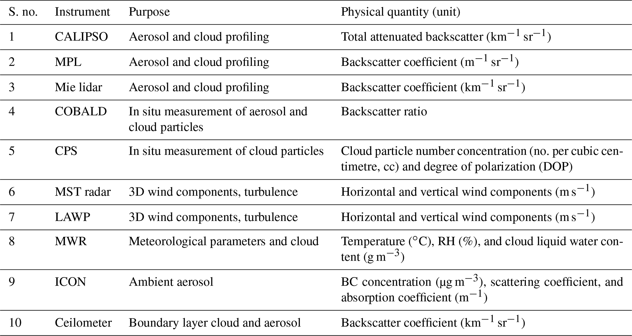
Table 1 lists the ensemble of instruments used in the campaign, their purpose, and the physical quantity that can be obtained from each instrument. Temporal variation in remote sensing data for the cloud and aerosol profiles is obtained from ground-based (MPL and Mie) lidars. Space-borne lidar (CALIPSO) also provide the same but for an along-track (roughly meridional) distribution near the time of overpass over Gadanki. In situ measurements of aerosol and cloud profiles and background meteorological parameters (temperature, relative humidity, wind speed and direction) are collected using the specialized balloon sounding (COBALD and CPS). Temporal variation in wind components obtained from the ground-based radars (MST radar and/or LAWP) aids in disentangling the effect of vertical winds and turbulence on aerosol–cloud interactions. An MWR provides the cloud liquid water and relative humidity profiles (among other variables), which are useful to constrain the cloud water content in a cloud layer and to understand the aerosol influence on cloud properties. In addition to these measurements, surface aerosol information obtained by the instrumentation available at the ICON observatory, NARL helps in understanding the role of sources of aerosol from the surface. Altogether, near-simultaneous information on the aerosol, cloud, and background meteorological conditions obtained from the multi-instrument set-up is used with the aim of understanding aerosol–cloud interactions.

Table 2 Date and time of the BACIS campaigns and the instruments operated during the corresponding campaigns.

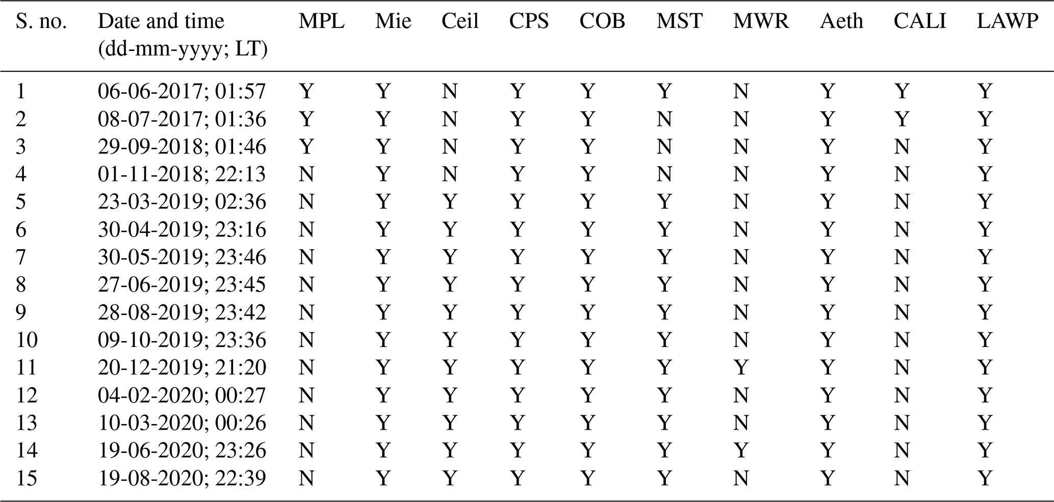
MPL stands for micro-pulse lidar; Mie stands for Mie lidar, Ceil stands for ceilometer, CPS stands for cloud particle sensor (CPS), COB stands for Compact Optical Backscatter AerosoL Detector (COBALD), MST stands for Indian MST radar, LAWP stands for lower atmospheric wind profiler, Aeth stands for aethalometer, CALI stands for CALIPSO, MWR stands for microwave radiometer.

Initially, when the experiment was being conceptualized, it was thought to conduct a launch once every 1 to 2 months. However, due to the limited number of specialized sondes (available to us), it was decided to instead conduct two pilot campaigns to demonstrate the proposed concept. A low-cost GPS- and GSM-based tracker is used for recovery purposes. Two pilot campaigns were conducted in the early hours of 6 June and 8 July 2017. Table 2 lists the date and time of all the balloon campaigns that were conducted from Gadanki as a part of BACIS and the instruments operated during the corresponding campaigns. As shown in Table 2, 15 launches were conducted from the 2017 to 2020. There was a manoeuver in the CALIPSO orbit during September 2018 (the CALIPSO track departed from A-Train to join C-Train; more details can be found at https://atrain.nasa.gov/, last access: 16 August 2022), followed by which we could not find the CALIPSO night-time passage close to Gadanki. There was also limited availability of, e.g. specialized sondes, compatible radiosondes, and GPS and GSM tracker assemblies. Because of these reasons, the rest of the campaigns were conducted on random dates. However, as seen in Table 2, we have managed to operate all the essential instruments proposed in the observational approach during other campaigns. Specifically, the campaigns in 2019 were conducted once a month (March to June 2019) or every 2 months (July to December 2019).

Figure 2 shows the photographs taken at the balloon facility (NARL) just before the launch during one of the campaigns. The balloon payload with specialized sondes (COBALD, CPS) and radiosondes (iMet and RS-11G) is shown in Fig. 2a and the pre-launch activities at the field are shown in Fig. 2b. As shown in Fig. 2a, the ozonesonde at the centre serves as the support for the balloon payload. A COBALD sonde with a slight upward-looking angle is attached to one side of the ozonesonde, and a CPS sonde is attached on another side. A radiosonde (Meisei and iMet) is connected to the remaining two sides. All the sondes are tightly packed using adhesive tape. At the base of the ozone sonde, a wide and thick thermocol sheet is arranged to protect the entire payload at the time of ground contact during descent. A couple of GPS- and GSM-based trackers are also attached to the payload alongside a power bank for safe recovery. The entire payload is hung on an inflated balloon with the help of a nylon thread. The length of the thread between the inflated balloon and parachute is 5 m, and the length of thread between the parachute and payload is 10 m. In this paper, CPS and COBALD data are shown at their actual resolution (5 m). However, in the estimation of the aerosol–cloud index, sensor data are averaged over the thickness of the cloud, which is about 300 m. Therefore, the sampling biases are nullified.

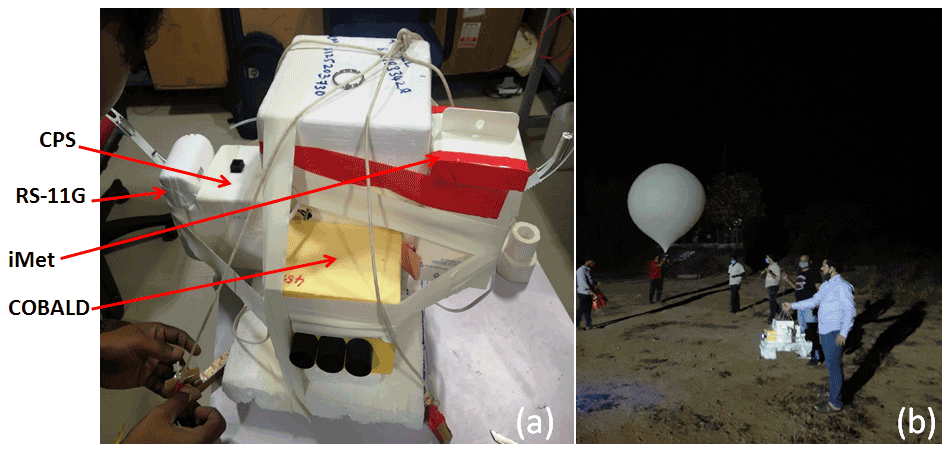
Figure 2 (a) The balloon payload with COBALD, iMet radiosonde, CPS, RS-11G radiosonde instruments attached. (b) Pre-launch preparations at the launch field with the payload and balloon visible.​​​​​​​

With the observational approach described above, the following scientific issues/objectives are being pursued and realized.

• i.

  The potential of the multi-instrumental observational approach for obtaining the information about the aerosol, cloud, and associated environmental parameters, such as 3D winds, relative humidity, and temperature simultaneously, is demonstrated.

• ii.

  Balloon-borne in situ measurements using a combination of space-borne and/or ground-based instruments are compared.

• iii.

  Aerosol and cloud are discriminated in a balloon sounding using the combined observations of COBALD and CPS sondes.

• iv.

  Aerosol–cloud interactions are verified and quantified, and an understanding of the influence of meteorological and dynamical parameters will be reached.

• v.

  The differences (if present) in the estimates of aerosol–cloud interaction using multiple instruments will be discerned, and the possible reasons for discrepancies will be discussed.

• vi.

  An understanding will be reached as to how the indirect effects of aerosols change radiative transfer through the atmosphere.

• vii.

  An assessment will be made of weather and climate model simulations using multi-sensor data.

2.4 Methods

2.4.1 COBALD data processing

Backscattered light received by COBALD is contributed by molecules, aerosols, and cloud particles in the atmosphere. The molecular Rayleigh contribution to the raw signal (cps) is established during the post-processing of the data using the simultaneous temperature and pressure recordings of the radiosonde. It serves to normalize the total signal in terms of backscattering ratio (BSR) according to

$$\begin{array}{}\text{(1)}& \mathrm{BSR}={\displaystyle \frac{{\mathit{\beta }}_{\mathrm{total}}}{{\mathit{\beta }}_{\mathrm{molecular}}}},\end{array}$$

where β_total and β_molecular are the backscatter coefficients corresponding to the contribution from particles plus molecules and only molecules, respectively. The sole particle contribution is obtained by BSR − 1, which expresses the ratio of the particle backscatter coefficient to the molecular backscatter coefficient. The uncertainty in the COBALD BSR is estimated to be 1 % and 5 % at the surface level and 10 km, respectively (Brabec et al., 2012; Vernier et al., 2015). The colour index (CI), referring to the particle backscatter only, is calculated from Eq. (2).

$$\begin{array}{}\text{(2)}& \mathrm{CI}={\displaystyle \frac{{\mathrm{BSR}}_{\mathrm{940}}-\mathrm{1}}{{\mathrm{BSR}}_{\mathrm{455}}-\mathrm{1}}}\end{array}$$

By definition, CI is an independent quantity of particle number concentration and is hence useful in interpreting the size of a particle. For analysis, COBALD raw data are binned into 1 hPa pressure levels. This could minimize noise and unwanted data and smoothen the profile. Figure 3 shows a typical example of COBALD data collected during the second campaign (8 July 2017). BSRs at 455 and 940 nm wavelength channels are represented by blue and red lines, respectively, while CI (derived using Eq. 2) is shown as a green line. From Fig. 3, a sharp increase in all parameters (BSRs at two channels, CI) found around 5 km associated with a thermal inversion (see the temperature profile in Fig. 3, shown in black) may be attributed to the presence of a low-level cloud or an elevated aerosol layer. Below ∼ 5 km, the BSR profile indicates tropospheric aerosol distribution. Within this altitude, BSR values around 2 km indicate boundary layer confinement. Note that there are no significant changes in CI within this 2 km height. Significant values in all parameters between 10 and 16 km are indicative of multiple high-level cloud layers. We have noticed that COBALD has captured profile information that was missing in the lidar data of the rest of the campaigns.

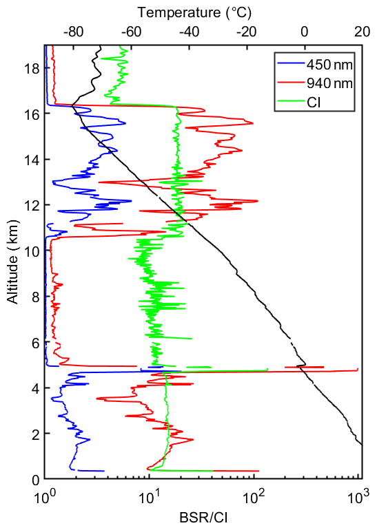
Figure 3 Backscatter ratio (BSR) at the 450 nm (blue) and 940 nm (red) channels were obtained using a COBALD sonde launched during the second pilot campaign (8 July 2017). The colour index (CI) estimated from BSRs at both channels is also shown (in green).

2.4.2 CPS data processing

The phase of the cloud particle detected by CPS is determined using a quantity called degree of polarization (DOP) given by the following relation:

$$\begin{array}{}\text{(3)}& \mathrm{DOP}={\displaystyle \frac{I_{\mathrm{55}}-I_{\mathrm{125}}}{I_{\mathrm{55}}+I_{\mathrm{125}}}}.\end{array}$$

Since the spherical particles (water droplets) do not provide significant voltage in the cross-polarization (I₁₂₅​​​​​​​ close to 0), the DOP values for such particles would be close to 1. On the other hand, the DOP for non-spherical particles (for example, ice crystals) would randomly take values between −1 and 1 as I₁₂₅ is non-zero and may or may not be greater than I₅₅. In addition to this, CPS can also detect the non-spherical particles in the lower troposphere with DOP values that may vary between −1 and 1.

The volume of the particle detection area within CPS is non-zero and estimated as ∼ 0.5 cm³ (see Sect. 2.3 of Fujiwara et al., 2016, for details). Therefore, when the particle number concentration is greater than ∼ 2 cm⁻³, more than one particle would exist simultaneously in the detection area, resulting in particle overlap and multiple scattering and thus a counting loss. The counting loss occurrence can be identified using a housekeeping parameter called “particle signal width”, defined as the time taken for the detection of a single particle. A simple correction of particle count using the particle signal width information is proposed by Fujiwara et al. (2016, see their Sect. 2.3 for the details) using a factor “f” which is as follows: (particle signal width in milliseconds) $/$ (1 ms). The raw counts from a CPS are corrected for multiple scattering and overlap effects using particle signal width data as in Eq. (4).

$$\begin{array}{}\text{(4)}& N_{\mathrm{corr}}=N_{\mathrm{meas}}\times \mathrm{4}{f}^{\mathrm{3}}\end{array}$$

Finally, the number of particles counted per second is converted to number concentration by assuming that the airflow at the CPS detection area is 70 % of the balloon ascent rate (see Appendices B and C of Fujiwara et al., 2016). The uncertainty of the number concentration when the above correction to the particle count is made (i.e. for the case of ≳ 2 cm⁻³) has not been evaluated by Fujiwara et al. (2016). It would be safe to assume that the estimated number concentration is valid in the representation of variations of the cloud properties rather than magnitude.

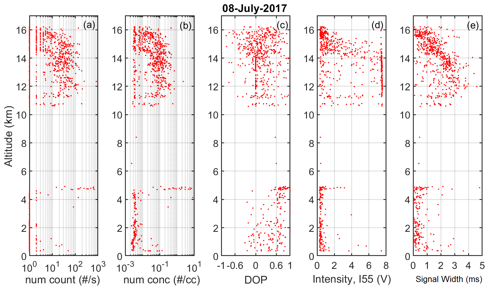
Figure 4 CPS measurements collected from the second pilot campaign (8 July 2017) showing (a) cloud particle number count (corrected) per second, (b) cloud particle number concentration per cubic centimetre, (c) degree of polarization of a cloud particle (DOP), (d) the intensity of light scattered at 55^∘ angle in volts, and (e) the particle signal width in milliseconds.

CPS data were analysed at their actual resolution of ∼ 5 m. Figure 4a shows the corrected cloud particle (number) count (based on Eq. 4) for the same day as shown in Fig. 3. Significant cloud particle count is found at around 5 km and from above 10 to 16 km. The number of particles counted per second at 5 km turns out to be high, suggesting the presence of a dense (optically thick) layer of low-level cloud. The corresponding cloud particle number concentration (cm⁻³) also represents (Fig. 4b) the cloud layers at the same altitudes. The DOP is estimated as per Eq. (3). In Fig. 4c, DOP values are found to be clustered in the region close to 1 at ∼ 5 km, indicating that the dense (low) cloud layer is a liquid cloud. On the other hand, the DOP values are randomly distributed between −1 and 1 in the altitude region of > 10 to 16 km, indicating that these are ice clouds. In Fig. 4d and e, particle signal width is often greater than 1 ms, and I₅₅ is sometimes ∼ 7.5 V for the ice cloud region between 11 and 14 km, suggesting particle overlap and multiple scattering, which might have led to signal saturation. This portion of the profile is more vulnerable to the data correction, which has been performed and shown in Fig. 4a.

2.4.3 Lidar data processing

Though the backscattered data at very high altitudes (> 30 km) are not significant, it is used as a background signal for noise correction. Range-corrected signal (RCS) from MPL and Mie is calculated from noise-corrected backscattered signal multiplied with a range square. In general, the RCS indicates the intensity of light backscattered from molecules, aerosols, and clouds in the atmospheric column. However, inversion techniques are commonly applied to the RCS with an assumption of lidar ratio (the ratio of extinction coefficient to backscattering coefficient) to obtain the profiles of total backscatter coefficient and the extinction coefficient of cloud and aerosol separately. Ground-based lidar data were analysed at their actual vertical resolutions. However, CALIPSO data were interpolated and processed at every 30 m resolution. This information is used in the discussion (Sect. 3.1).

2.4.4 Estimation of saturation relative humidity

Two dedicated radiosondes from iMet and Meisei were employed in the balloon campaigns for the measurement of meteorological parameters (temperature, pressure, relative humidity, and horizontal winds with height) and to act as an interface with COBALD and CPS specialized sondes, respectively. As mentioned, temperature and pressure profiles from the radiosonde were used in the post-processing of the COBALD sonde to scale the signal to the molecular Rayleigh scattering. In addition to this, radiosonde temperature and relative humidity are useful in understanding the state of saturation of water vapour in the column. By convention, relative humidity reported from radiosonde is always over the plane surface of liquid water (because radiosonde relative humidity sensors are factory calibrated) even below 0 ^∘C. This is because water droplets may exist even below 0 ^∘C and down to −30 to −40 ^∘C (in the form of supercooled liquid) in the atmosphere. Saturation relative humidity (SRH) is defined in Fujiwara et al. (2016; see also Fujiwara et al., 2003) as the ratio of saturation vapour pressure over the plane surface of ice (e_si) to water (e_sl), expressed in units of percentage, and can be a good metric to describe the state of water vapour in the atmosphere, such as sub-saturation, saturation, and/or super-saturation, particularly at air temperatures below 0 ^∘C (with respect to ice). In this study, both e_sl and e_si are calculated using the Hyland and Wexler formulation (see Appendix A of Murphy and Koop, 2005) by using radiosonde temperature data. For temperatures warmer than 0 ^∘C, water vapour saturation is indicated by 100 % RH. For temperatures colder than 0 ^∘C, water vapour is said to be saturated if RH ≅ SRH and super-saturated when RH > SRH. This information is used in the discussion (Sect. 3.2).

2.4.5 Discrimination of cloud and aerosol in a balloon profile

COBALD measurement always represents backscatter light from the combination of aerosol and cloud. Obtaining only information on aerosol is not possible (for COBALD) in the presence of clouds, and the corresponding regions have to be identified and rejected. This cloud clearing has been established previously for studies related to the upper troposphere–lower stratosphere (UTLS) region (Vernier et al., 2015, 2018). In contrast, COBALD was used for cloud investigation in combination with the Cryogenic Frost point Hygrometer (CFH) to identify supersaturation (with respect to ice) below, above, and within cirrus clouds to improve the understanding of microphysical processes in cirrus clouds (Cirisan et al., 2014). This sonde also detected volcanic aerosol tracers in the stratosphere (Vernier et al., 2020). The Asian Tropopause Aerosol Layer (ATAL) is a well-documented phenomenon occurring in the UTLS region during the summer monsoon season in South Asia. Vernier et al. (2015) proposed two cloud-clearing methods for discrimination of aerosol from cirrus clouds in the ATAL region using the physical quantities of colour index (CI), relative humidity over ice (RHi), and backscatter ratio (BSR) at 940 or 532 nm (the latter was interpolated from the 455 nm data for inter-comparison with CALIOP). In the presence of CFH data, the RHi cloud-filtering approach classifies ATAL and UTLS aerosol layers using as having a BSR (at 532 nm) < 1.3 and RHi < 70 %. For measurements of COBALD alone, the CI method indicates clouds with CI < 7 and a BSR (at 940 nm) < 2.5. It was shown that both methods effectively discriminate ATAL aerosol from upper-tropospheric thin clouds. Brunamonti et al. (2018) also applied the cloud-clearing criteria (BSR at 940 nm < 2.5, CI < 7, and RHi < 70 %) following Vernier et al. (2015) and found a clear signal of enhanced BSR (at 455 nm) between 1.04 and 1.12 indicative of the aerosol population in the ATAL region. However, it is noted that the methods proposed by Vernier et al. (2015) and Brunamonti et al. (2018) were developed for the UTLS aerosol, and their applicability to COBALD measurements of boundary layer and/or mid-tropospheric aerosol needs to be validated.

In the present study, we made use of a CPS sonde in tandem with COBALD. As already mentioned, CPS is sensitive to particles in the size range of > 2 µm, and hence it detects cloud particles (both liquid droplets and ice crystals) and sometimes coarse-mode aerosol particles (such as dust) of these sizes. Fujiwara et al. (2016) have demonstrated the potential of a CPS sonde in detail using balloon sounding carried out at a mid-latitude site (Japan) and at tropical sites (Indonesia). Narendra Reddy et al. (2018) used a CPS measurement from Gadanki to validate their method of retrieving cloud vertical structures based on radiosonde measurements. Therefore, to better segregate the clouds from aerosols in the COBALD measurements, the CPS sonde has an added advantage compared to methods as described by Vernier et al. (2015) and Brunamonti et al. (2018). This implies wherever the cloud is present in a profile, CPS identifies it (along with its phase), and the corresponding COBALD particle backscatter data refers to the cloud. The rest of the particle signals in the COBALD profile should correspond to aerosol. However, it may also correspond to the (thin) cloud that might have been missed or undetected by a CPS. Thus, identification of aerosol and cloud in an altitude profile is the key measurement of this paper. The concept is illustrated in Sect. 3.2.

2.4.6 Estimation of aerosol–cloud interaction index

Balloon data from all campaigns can be pooled to explore the aerosol–cloud relationship. For this purpose, a simple scheme is developed to carry out the required computations. CPS profile data are checked for a cloud layer in the altitude regime of liquid or low-level clouds (below 5 km). As already discussed, CPS also identifies particles that are non-spherical in nature. To separate cloud particles from non-spherical particles, the following conditions have been imposed on various CPS measured parameters. Cloud particle count should be > 10 s⁻¹, cloud droplet number concentration should be > 10⁻³ per cc, DOP should be > 0.6, relative humidity should be > 95 %, and temperature should be > 0 ^∘C. As there is a chance of randomly distributed data points in the measurement column satisfying the above conditions, we considered only those points present continuously up to a minimum thickness of 100 m (with at least one point for every 40 m). Further, COBALD data of blue backscatter 100, 200, 300, 400, and 500 m below the cloud base has been picked up separately (for the same profile) as a proxy of aerosol to check its influence on the cloud above. As already mentioned, post-processed data of backscatter ratio from the COBALD sonde represents the contribution from both molecule and particle (cloud and/or aerosol). Hence, the particle backscatter ratio is obtained by subtracting the backscatter ratio from 1. To avoid high values of particle (blue) backscatter ratio possibly originating from the interaction with high relative humidity usually expected near to cloud base (boundaries), we have adopted two methods. First, high values of particle (blue) backscatter below the cloud base are removed if they are beyond a threshold value of 3.15. The threshold is arrived at using a box plot (figure not shown) drawn for the entire particle backscatter data set (for sounding with clouds) from cloud base to 500 m below, and it is found that 3.15 corresponds to the upper whisker ($Q\mathrm{3}+\mathrm{1.5}\times (Q\mathrm{3}-Q\mathrm{1})$). Further, the particle backscatter data are corrected for relative humidity in cases where a statistically significant (p value ≦ 0.05) and good correlation (> 0.71) is found among relative humidity and particle backscatter ratio. A typical example from the scheme is shown in Fig. 5 for the launch conducted on 1 November 2018, which depicts cloud layers, blue particle backscatter ratio below the cloud and aerosol backscatter ratio (shaded black dots). The scheme is applied to the balloon sounding and the results are discussed in Sect. 3.4.

Figure 5 The top row shows COBALD (red dots) and CPS (blue dots) observations from a sounding held on 1 November 2018 up to the altitude of 6 km (as the focus is on the liquid cloud region). The bottom row shows the same parameters but for the portion of the same profile where liquid cloud (blue dots) and aerosol (from cloud base to 500 m below) were identified by the scheme.

Aerosol–cloud interaction can be quantified based on an index (ACI) using three methods discussed in Feingold et al. (2003, 2006). ACI is defined as the slope of the linear fit between the logarithm of cloud proxies such as cloud optical depth, cloud particle radius and cloud droplet number with the logarithm of aerosol proxy. ACI in this study has been estimated using the Eq. (5).

$$\begin{array}{}\text{(5)}& \mathrm{ACI}={\displaystyle \frac{\mathrm{d}\log N_{\mathrm{c}}}{\mathrm{d}\log {\mathrm{BSR}}_{\mathrm{b}}}}\end{array}$$

Where cloud droplet number count (N_c) is taken as cloud proxy, whereas COBALD (blue) particle backscatter is (BSR_b) taken as aerosol proxy. It is to be noted that cloud particle count is used here to represent cloud property instead of droplet number concentration as the former is a direct measurement (of CPS). The slope of the linear fit between the natural logarithm of N_c and BSR_b indicates the magnitude of the aerosol–cloud interaction (ACI index), which should be between 0 and 1 (Feingold et al., 2003). Note the condition shown in Eq. (5) is independent of the liquid water path as it verifies/quantifies the aerosol activation process.

2.4.7 Uncertainty in ACI estimation

The uncertainty in ACI stems from uncertainties in both the COBALD backscatter ratio and CPS cloud particle counts. The slope of the curve (linear fit of data on a log–log scale) can be written as a function of BSR_b (blue backscatter ratio) and N_c (cloud particle count) as

$$\begin{array}{}\text{(6)}& \mathrm{ACI}=f({\mathrm{BSR}}_{\mathrm{b}},N_{\mathrm{c}})={\displaystyle \frac{\log N_{\mathrm{c}}-C}{\log {\mathrm{BSR}}_{\mathrm{b}}}},\end{array}$$

where “C” is the intercept of the curve. The partial derivative of f(BSR_b, N_c) indicates uncertainty in ACI with respect to uncertainty in individual parameters (N_c and BSR_b). The combined uncertainty (UC) in ACI is given by the following equation:

$$\begin{array}{}\text{(7)}& \begin{array}{rl}& \mathrm{UC}=\\ & \sqrt{{\left({\displaystyle \frac{\partial f({\mathrm{BSR}}_{\mathrm{b}},N_{\mathrm{c}})}{\partial {\mathrm{BSR}}_{\mathrm{b}}}}\right)}^{\mathrm{2}}(u{\mathrm{BSR}}_{\mathrm{b}}{)}^{\mathrm{2}}+{\left({\displaystyle \frac{\partial f({\mathrm{BSR}}_{\mathrm{b}},N_{\mathrm{c}})}{\partial N_{\mathrm{c}}}}\right)}^{\mathrm{2}}(u{N}_{\mathrm{c}}{)}^{\mathrm{2}}}\end{array},\end{array}$$

where uBSR_b and uN_c are individual uncertainties.

3 Results

3.1 Comparison of balloon measurements

It is important to know the performance of these sondes in comparison to other measurement techniques. Here, we make use of data from two pilot campaigns to demonstrate the consistency of balloon-borne measurements with those of ground-based and space-borne remote-sensing instruments. As mentioned previously, the first two (pilot) campaigns have been conducted in line with the proposed concept.

3.1.1 Pilot campaign 1 (launch held on 6 June 2017 at 01:50 LT)

The CALIPSO satellite overpass time for the first pilot campaign was around 02:00 LT on 6 June 2017 (starting time of the track). The balloon was launched at 01:50 LT on the same day just before CALIPSO overpass time. Combined measurements from specialized balloon-borne sondes and ground-based and space-borne lidars obtained during the first launch of the campaign are shown in Fig. 6.

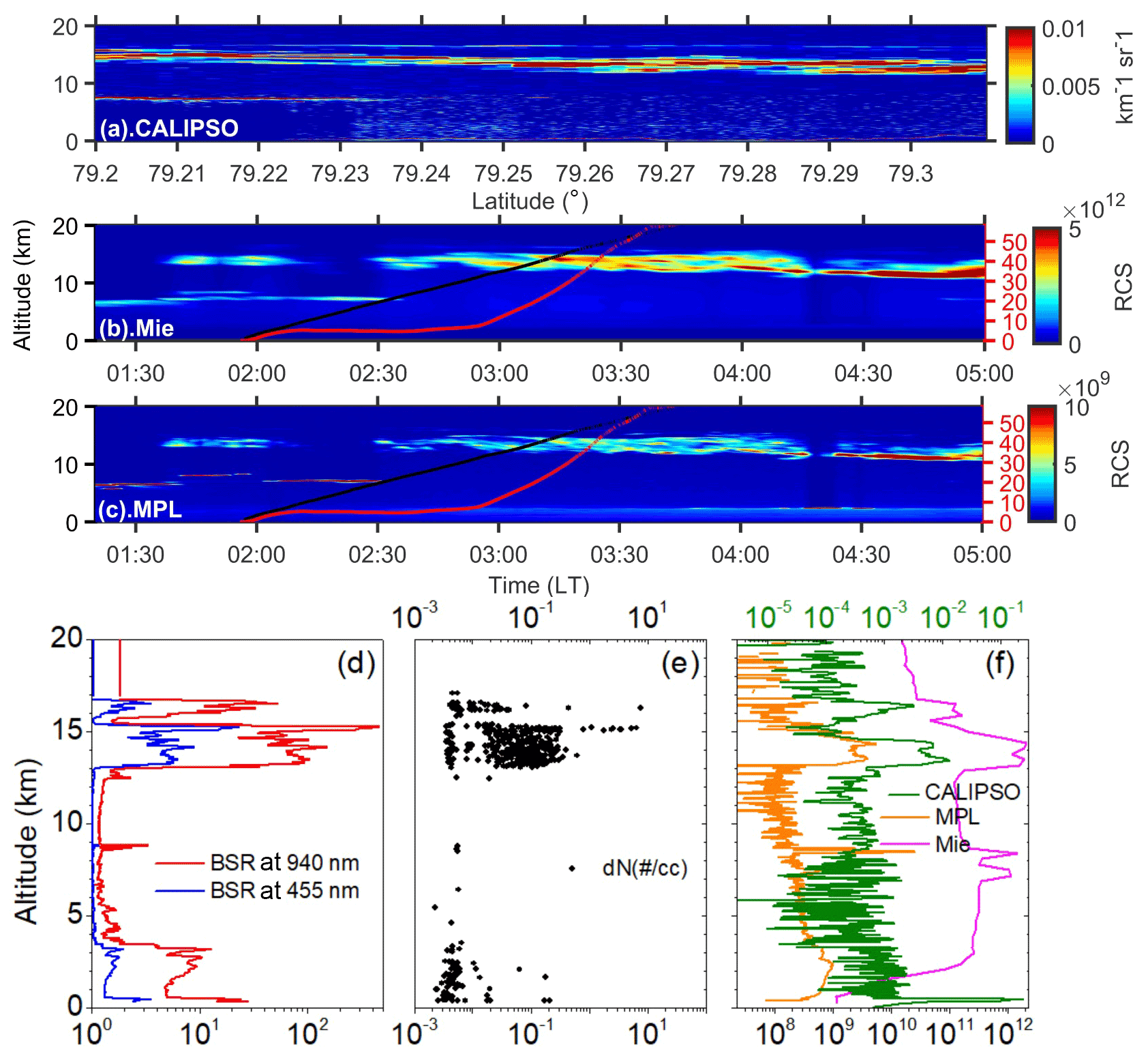
Figure 6 Multi-instrument data from a balloon sounding held in the early hours of 6 June 2017. The total attenuated backscatter from (a) CALIPSO and temporal variation in the range-corrected signal from (b) Mie lidar and (c) MPL. The red (black) lines overplotted on contour maps (b) and (c) represent balloon drift (altitude) in kilometres with time. Drift as a function of time can be read with the right y axis (red font), and altitude as a function of time can be read with the left y axis. (d) The profiles of BSR at two channels from COBALD (blue and red lines); (e) particle number concentration from CPS (black dots); and (f) RCS from MPL (orange), Mie lidar (magenta), and total attenuated backscatter from CALIPSO (olive green).

The BSR from the COBALD sonde at 455 nm (950 nm) is plotted in Fig. 6d as a blue (red) line. BSR from both channels is referenced to the same x axis scale. Similarly, cloud particle number concentration (dN, no. per cc) from CPS sonde is plotted as black dots (Fig. 6e). On the other hand, range-corrected signal (RCS) from ground-based lidars (Mie, MPL) is averaged over a short period during the CALIPSO overpass and plotted in magenta (averaged from 01:50 to 02:00 LT) and orange (averaged from 01:50 to 01:55 LT) lines, respectively (Fig. 6f). The total attenuated backscatter (km⁻¹ sr⁻¹) from CALIPSO is also averaged for the profiles found nearest to the location and shown as an olive green line (Fig. 6f). The significant peaks in physical quantities being compared among the different measurements are representative of responses from clouds and aerosols in the atmosphere. At this point of discussion, we have not distinguished their contributions. The balloon drifts away from the launch location with time; therefore, it is also required to check the degree of co-location of measurements with the lidars. To facilitate this, a portion of nocturnal variation (representing the balloon launch duration) in range-corrected signal from both Mie and MPL is shown in Fig. 6b and c, respectively. The CALIPSO overpass track consisting of 166 profiles is also plotted as a function of longitude (Fig. 6a). For the sake of easy identification of simultaneous lidar measurements, the balloon indices such as height and drift (radial distance from launch location) are overplotted as a function of time on contour maps as shown in black and red lines, respectively (Fig. 6b and c).

Balloon-borne in situ measurements from COBALD and CPS show significant peaks in the lower troposphere (below 4 km) and upper troposphere (between 13 and 17 km) at the same altitude regions. It can be seen from Fig. 6d and c that there is a good resemblance between the in situ and MPL measurements in the lower troposphere (below 4 km). This is because there is almost no change in the atmospheric conditions as the balloon took approximately 15 min to reach an altitude of 4 km with a radial distance of 5 km away from the launch location. Mie lidar information is not reliable for this altitude region (below 4 km) as it is not in the overlapping region of the telescope viewing geometry and laser beam dispersion (see Sect. 2). The CALIPSO signal also looks to be dispersed and noisy for this altitude region. This could be due to the attenuation of the signal from the top side layers as seen in Fig. 6a at a longitude of 79.24^∘ E (the nearest profile's longitude).

Next to this is the sharp peak seen in the COBALD red channel at slightly below 9 km (Fig. 6d). This can again be seen in Mie and MPL profiles (Fig. 6b, c) but at 8.4 km (slightly below cloud detection height). However, it should be noted that these profiles are averaged for a short duration of time during the CALIPSO overpass. There is another peak in the Mie lidar profiles at ∼ 7.2 km (Fig. 6b) that is not seen in COBALD. It is approximately 45 min (around 02:45 LT) from the time of launch when the balloon reached the altitude of ∼ 9 and 5.8 km away before detecting a sharp peak. As there is no significant range-corrected signal during this time and altitude in the ground-based lidar data (Fig. 6b and c), the sharp layer detected by COBALD may be a localized cloud layer or a passing layer that might have ascended or descended. Exact attribution can be made with a detailed study, but it is beyond the scope of the current analysis.

Further, the balloon drift was within a 10 km range until 03:00 LT, when it reached heights of ∼ 12 km. This implies weak horizontal winds and thus also weakly associated wind drifts. Thereafter, the balloon started drifting rapidly due to high wind speeds between 10 and 20 m s⁻¹. The in situ measurements of both COBALD and CPS show strong double peaks from ∼ 13–15.5 and 16–16.5 km (Fig. 6d, e). Profiles from Mie, MPL, and CALIPSO measurements also showed similar peaks, but for MPL the upper-side peak is missing (Fig. 6f). It may be once again noted that these profiles are averaged for a short duration of time during the CALIPSO overpass, and the return signal from MPL at high altitudes (∼ 16 km) during the same time period suffered severely due to the presence of a mid-tropospheric cloud layer (at ∼ 7 km) as seen in Fig. 6c. This is not the case for the return signal from Mie lidar as the power and energy of the Mie laser are relatively high (Fig. 6b). However, strong double-peak structures can be noticed in the simultaneous observations of both ground-based lidars (Mie and MPL) at similar heights during the time corresponding to the balloon altitude of 13 km (after 03:00 LT). Therefore, the same upper-tropospheric cloud layers being detected in the ground-based, space-borne, and in situ measurements suggests that they are extended cloud layers. Dynamical aspects of the southwest monsoon over the sub-continent refer to the presence of the Tropical Easterly Jet (TEJ), which is strong enough to swipe anvil clouds of mesoscale convective systems thousands of kilometres (Sathiyamoorthy et al., 2013).

3.1.2 Pilot campaign 2 (launch held on 8 July 2017 at 01:35 LT)

The starting time of the CALIPSO overpass track for the second pilot campaign was at 02:00 LT. The balloon was launched at 01:35 LT, nearly 30 min before the starting time of the CALIPSO overpass. Data from all the instruments are plotted in Fig. 7, which is presented in the same way as Fig. 6. MPL and Mie profiles were averaged from 01:50 to 02:00 LT (close to the CALIPSO overpass time over Gadanki).

Figure 7 The same as Fig. 6 but for the second pilot campaign (8 July 2017).

The observations from COBALD and CPS match reasonably well (Fig. 7d, e), as significant peaks were found in the lower troposphere (0–5 km) and upper troposphere (10–16 km). The profiles from space-borne and ground-based lidars (Fig. 7f) also show a similar response as in situ measurements (both in the lower and upper troposphere), but lidar measurements exhibit additional peaks in the mid-troposphere (between 5 and 10 km). It should be noted that profiles from lidar measurements are averaged over a short period, as mentioned above.

Simultaneous observations from both the space-borne (CALIPSO) and ground-based (Mie and MPL) lidars are shown in Fig. 7a, b, and c. Due to high wind speeds (10–20 m s⁻¹), the balloon drifted about 5 km away from the launch site while crossing the boundary layer height (∼ 2 km). The features found within the boundary layer as measured by in situ instruments (Fig. 7d) are in agreement with those of MPL measurements (Fig. 7c) for the same altitude region. Note that Mie lidar measurements are not reliable at these low altitudes and that CALIPSO has not yet started passing by the launch site. The balloon continued to drift away but with a reduced wind speed of 10 m s⁻¹. At around 4.3 and 4.7 km (10 km away from the launch site), the balloon detected two layers (strong peaks). The time corresponding to this balloon height was around 01:50 LT, and at this point two layers can also be seen in both the ground-based lidars at the same altitudes (Fig. 7b and c), indicating the presence of an extended layer (evident in both the in situ and ground-based measurements). The layer at 4.7 km was also noticeable in the CALIPSO profile measurements (Fig. 7a). This is because the CALIPSO started coming close to the site when the balloon was at this height, and the CALIPSO profile corresponds to an average of (nearest) profiles at around 79.32^∘ E longitude (Fig. 7a). Further, the balloon started drifting towards the launch site until it reached a height of ∼ 7.5 km at a distance of ∼ 13 km away. While moving towards the site, the balloon started detecting the layers starting from 11 km. The time corresponding to the balloon height of 11 km is around 02:45 LT, and at this point in time simultaneous MPL data show almost weak returns (Fig. 7c), whereas the Mie lidar shows a better return signal (Fig. 7b) than MPL. In continuation of this, the balloon started drifting further toward the site until it reached as close as ∼ 3.5 km at a height of ∼ 12.5 km. Thereafter, it started moving rapidly away from the location with high wind speeds due to the characteristic of TEJ. Multiple layers of clouds have been nicely captured by in situ measurements from 11 to ∼ 16 km. However, prominent lidar returns were not noticeable in the simultaneous observations of Mie and MPL. This is because of a strong lower-tropospheric cloud layer present at around 5 km limiting the detection of upper-tropospheric cloud layers by both ground-based lidars. However, all of these layers were prominently captured in CALIPSO observations as they use top-down laser probing.

In summary, the data from both pilot campaigns illustrate the limitations of the ground-based and/or space-borne lidars in detecting the complete cloud vertical structure. At the same time, in situ data emphasize reasonable agreement of the balloon-borne measurements with the ground-based and space-borne measurements and add to the remote sensing techniques while detecting the missing portion of the cloud vertical structure.

The observational facilities at NARL are shown in Fig. 8. A typical example of high-resolution vertical wind measurements obtained from MST radar on 8 July 2017 is shown in Fig. 9f, and profiles of all the three-dimensional winds averaged between 02:30 to 03:30 LT are shown in Fig. 9a–c to compare the wind measurements. We also superimpose the zonal and meridional winds in the respective panels obtained from radiosonde for comparison. Consistency in the measured winds between these two independent techniques can be noticed. Since this campaign falls during the Indian summer monsoon season, easterly wind velocities exceeding 50 m s⁻¹, i.e. the TEJ, can be noticed between 14 and 16 km in altitude as a part of synoptic-scale systems (Fig. 9a). In addition, zonal winds are westerly and are also part of a large-scale monsoon system. These winds play a crucial role in bringing clouds and aerosol from far away sources. In general, meridional winds are weaker and more southerly (Fig. 9b). Vertical winds mostly show updraughts, except in the UTLS region where downdraughts are noticed (Fig. 9c), and similar features persist through this campaign (Fig. 9f). Occasional patches of updraughts and downdraughts can be noticed during the campaign, which is associated with monsoon convection. These vertical winds act in the upliftment of aerosol and clouds. Enhanced signal-to-noise ratio (SNR) layers are also noticed (Fig. 9d) at a few altitudes and are mostly related to large temperature and water vapour gradients that generally occur in the presence of clouds. Doppler width (Fig. 9e) shows higher values below the boundary layer and the UTLS region, suggesting active turbulence.

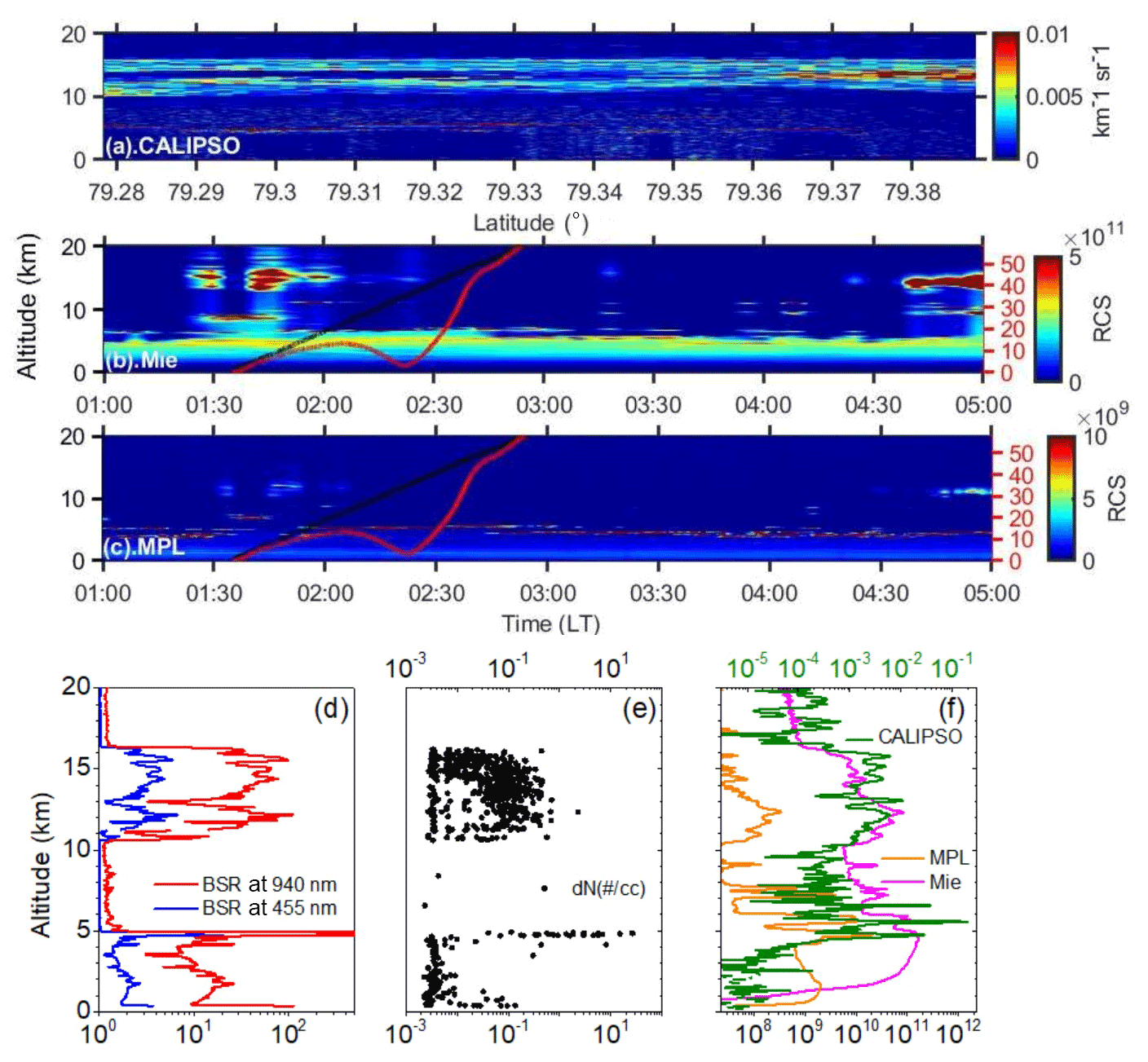
Figure 8 Map of the balloon launch facility and remote sensing apparatus at NARL (from Google Maps). Imagery © 2022 CNES/Airbus, Maxar Technologies, Map data © 2022.

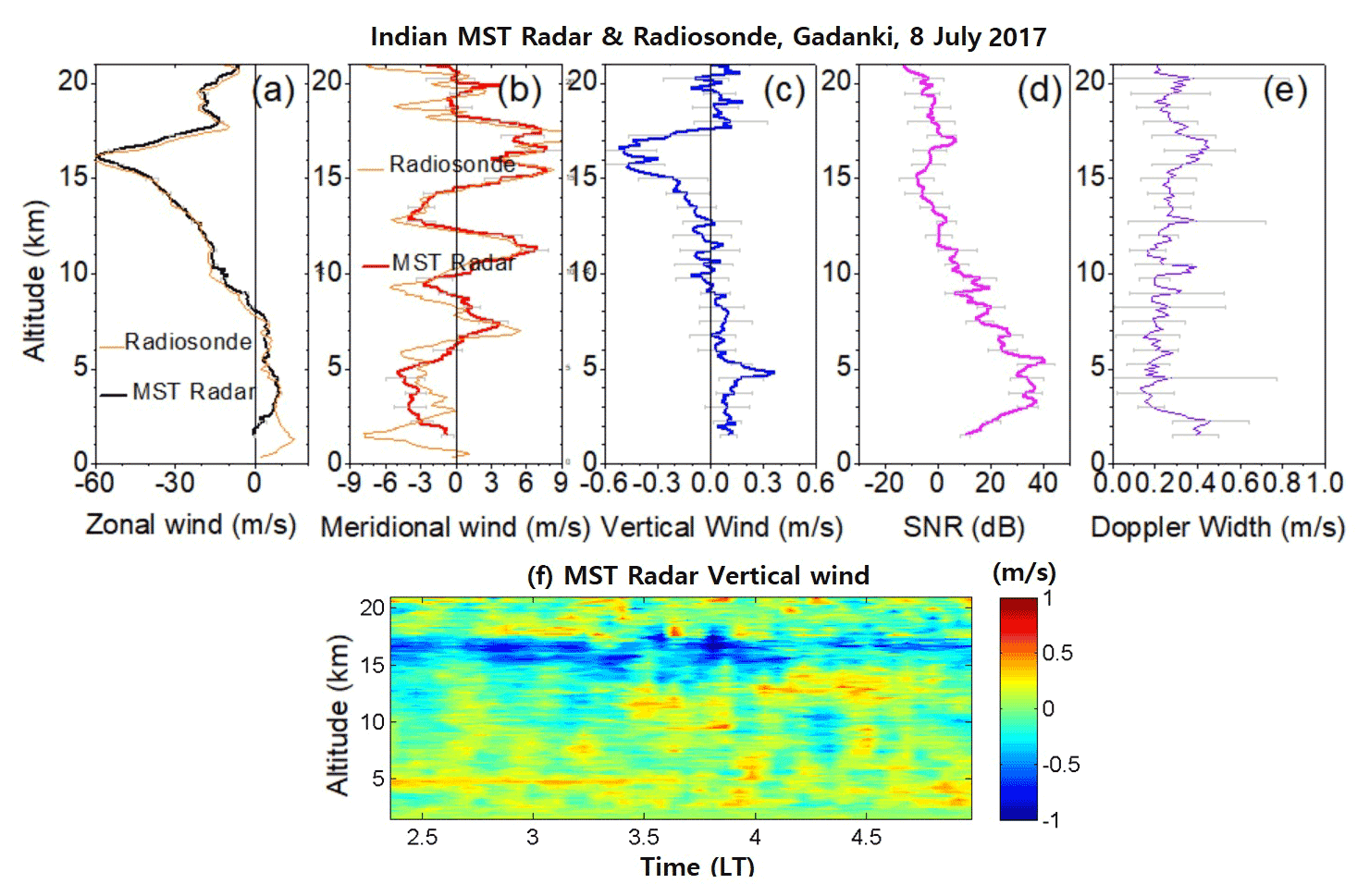
Figure 9 Profiles of (a) zonal wind, (b) meridional wind, (c) vertical wind, (d) signal-to-noise ratio (SNR), and (e) Doppler width obtained from Indian MST radar on 8 July 2017 and averaged during 02:30 to 03:30 LT. Horizontal bars show standard deviation. Radiosonde-observed zonal and meridional winds are also superimposed in the respective panels. (f) Time–altitude section of vertical wind obtained from Indian MST radar during the radiosonde launch time.

3.2 Interpretation of aerosol and cloud features in a balloon profile

To fulfil the primary objectives of the campaign, it is a priority to distinguish aerosol and cloud in a balloon-borne in situ profile. In connection with this, combined measurements of CPS and COBALD from a balloon sounding held on 27 June 2019 at 23:30 LT are interpreted as shown in Fig. 10. This particular sounding is selected because it showcases all of the features that can be detected by a CPS sonde in a profile, such as liquid cloud, supercooled liquid cloud, ice cloud, and non-spherical particle layers. INSAT3D brightness temperature, shown in Fig. S1 in the Supplement, indicates the evolution of a localized cloud system north of the observational site initiated a few hours before the launch and eventually spreading over the site.

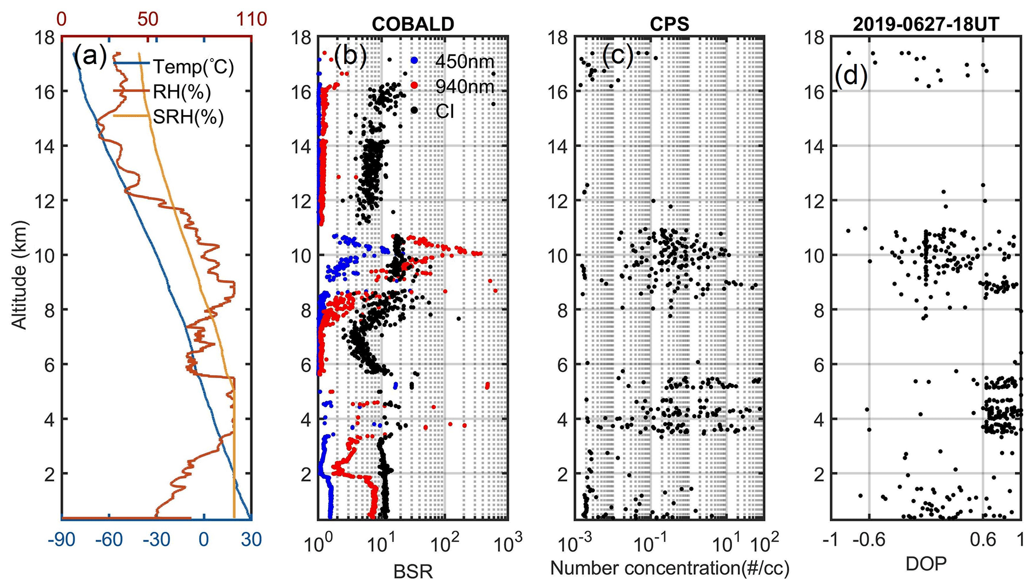
Figure 10 Combined observations of COBALD and CPS from balloon sounding held on 27 June 2019 at 23:30 LT: (a) temperature (T), relative humidity (RH), and saturation relative humidity (SRH); (b) backscatter ratio at 455 nm (blue) and 940 nm (red) and colour index (black); (c) cloud particle number concentration; and (d) degree of polarization (DOP).

To characterize the background conditions of the atmosphere, meteorological parameters such as relative humidity (RH) and temperature (T) obtained from RS-11G radiosonde are plotted in Fig. 10a (red and blue lines). In Fig. 10a, SRH is also shown (yellow). The SRH and RH can be read from the same top x axis (in red) as shown in Fig. 10a.

The CPS sonde usually features clouds that can be better identified with the information based on DOP, and corresponding profiles of T, RH, and SRH. From Fig. 10d, DOP values close to 1 (from 0.6 to 1) are noticeable at different altitude ranges in the profile, i.e. 3.5 to 5.5 and 8.6 to 9 km, and DOP values are spread (−1 to 1) between 9 and 11 km. In the altitude range from 3.5 to 5.5 km, CPS detected multiple liquid cloud layers, corresponding to the multiple layers of 100 % RH. However, the corresponding COBALD blue and red backscatter data points are limited (Fig. 10b). This is because COBALD backscattered signals showed missing values due to saturation of photodiodes in the presence of thick liquid cloud layers; these had to be removed during post-processing of the data and are not discussed further.

The layer extending between 3.5 and 3.8 km (300 m thick) is observed with RH and T in the range 99 %–100 % and 7–8.7 ^∘C, respectively, indicating saturation of water vapour with respect to liquid (RH ≅ SRH) that is conducive to the formation of a (liquid) cloud. Further, the majority of droplet number concentrations in this liquid cloud layer range between 0.1 to 1 cm⁻³. A rough estimate of particle size information (water droplet or ice crystal) can be inferred from CPS voltage data (I₅₅). According to Fujiwara et al. (2016), I₅₅ mostly lying below 1 V suggests that these droplets are sized ∼ 2–13 µm. Another liquid cloud layer extending from 4 to 4.4 km (400 m thick) is observed with vapour saturation over liquid (100 % RH) and temperatures from 3–6 ^∘C. CPS shows that droplet number concentration peaks in the range 0.1–10 cm⁻³ with the highest in 0.1–1 cm⁻³. The intensity (I₅₅) values (< 1 V) indicate that the majority of droplet sizes are ∼ 2–13 µm. The third liquid layer in the range of 3.5 to 5.5 km is observed between 5.1 and 5.5 km (400 m thick), with the highest droplet number concentrations in the range of 0.1–10 cm⁻³ and sized around 2–13 µm (I₅₅ < 1 V). However, RH observations show 100 % RH or RH > SRH, i.e. water vapour super-saturated over ice at temperatures slightly below 0 ^∘C (0 to −3 ^∘C), suggesting that the cloud layer may be composed of supercooled liquid droplets. Another clear supercooled cloud layer was detected between 8.6 and 9 km (400 m thick) with super-saturation of vapour over ice at 100 % RH or RH > SRH and −21.5 to −23.5 ^∘C temperatures. The observed features of droplet number concentration and particle size are similar to those of the supercooled cloud found in the lower atmosphere. The only difference that could be noticeable is in the distribution of DOP values shown in Fig. S2, which indicates the tendency of droplets toward non-sphericity in the mid-tropospheric supercooled liquid cloud. COBALD signals were found to be limited for all liquid and supercooled layers discussed above.

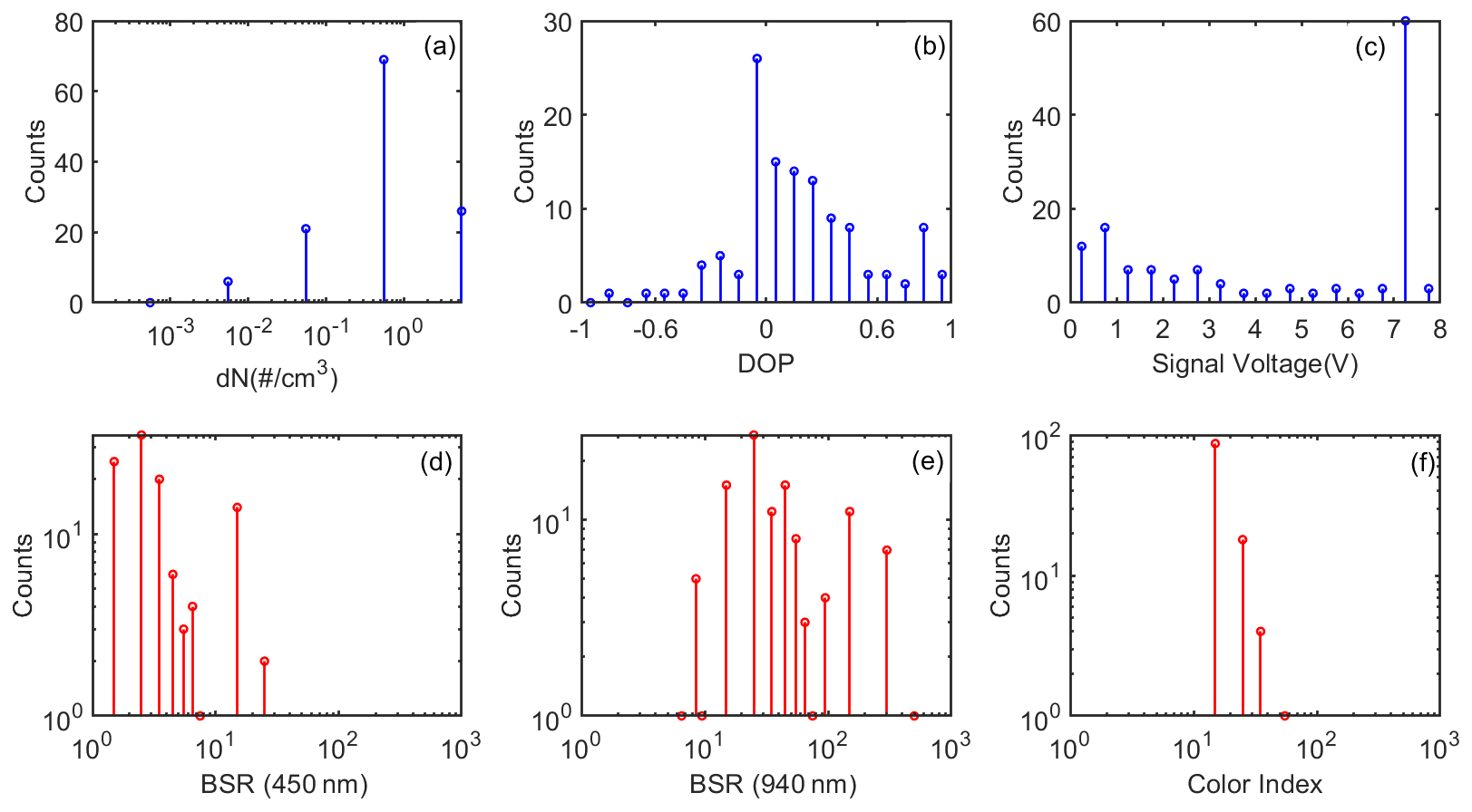
Figure 11 Histogram of (a) droplet number concentration (dN) in no. per cc, (b) degree of polarization (DOP), (c) backscattered signal (volts), (d) backscatter ratio at 455 nm, (e) backscatter ratio at 940 nm, and (f) colour index. Panels (a–c) and panels (d–f) respectively show CPS data and COBALD data for the ice cloud layer between 9 and 11 km from the sounding held on 27 June 2019.

The topmost layer in the upper troposphere (spreading from 9.5 to 11 km) is an ice cloud layer as per its DOP values. The temperatures within the cloud are found in the range of −22 to −40 ^∘C. RH values are > SRH, suggesting the super-saturation of vapour (over ice) within the ice cloud. The histogram of data for all the parameters obtained from COBALD and CPS for this ice cloud layer (9–11 km) is shown in Fig. 11. The number concentration of ice cloud particles (Fig. 11a) lies between 0.01 to 10 cm⁻³, with a peak in the range of 0.1–1 cm⁻³. Non-sphericity of particles is seen by the wide distribution of DOP values in the range −0.4 to 1, with the majority of them lying close to 0 (Fig. 11b). In particular, DOP values close to 0 indicate (see Sect. 2) that both plane and cross-polarization intensities of scattered light (I₅₅ and I₁₂₅) are comparable. This happens when both detectors get saturated due to a large number of small-sized particles, a few large-sized ice particles, or both. In support of this, the I₅₅ values (Fig. 11c) are found to peak in the 7–8 V range (∼ 7.5 V) for such cases. Further, if saturation voltages are due to large size, they may correspond to ice particles that ∼ 80–140 µm or greater in size (corresponding to I₅₅ of ∼ 7.5 V), assuming that the results from laboratory experiments by Fujiwara et al. (2016) using standard spherical particles can be applied for these ice clouds. Apart from this, the second peak in I₅₅ noticed below 1 V corresponds to ice particles sized between roughly 2 and 14 µ m.

The COBALD BSR corresponding to this ice cloud is symmetrically distributed from 1–10 and 10–100 for blue (Fig. 11d) and red (Fig. 11e) wavelengths, respectively. However, there are some observations that are beyond 10 (100) at blue (red) wavelengths. Similarly, the CI for this cloud (Fig. 11f) is found mostly between 10 and 20, but for a few instances it is observed from 20 to 40. From the definition (see Sect. 2), the CI is independent of the number concentration, and hence it can be used as an indicator of the mode radius of particles. With the assumption of the single-mode log-normal size distribution of spherical aerosol and cloud particles, Mie calculations show CI is 4–10 for small particles of mode radius up to 1–2 µm and 14–20 for large particles of 2–20 µm. CI converges to around 20 as a geometric limit for very large particles of mode radius ≳ 50 µm. However, CI can have values > 20 at mode radius 2–20 µm as CI is a non-monotonous function of mode radius and exhibits Mie oscillations (due to variations of scattering efficiencies with size parameter). The amplitude and frequencies of Mie oscillations depend on the width of the log-normal size distribution assumed. For example, at a width higher than 2 (representing polydisperse aerosol populations), these oscillations are mitigated and lead to a monotonous dependency of CI and mode radius. For stratospheric aerosols in the size range of 0.02–0.4 µ m, the CI is found to be in the range of 5–7 (Rosen and Kjome, 1991). This is because stratospheric aerosols exhibit size distributions with narrow standard deviations. Aerosol size distributions in the UTLS region may also be assumed as log-normal (similar to stratospheric aerosols); hence, the criteria CI < 7 might be suitable for cloud filtering in the ATAL region (see Sect. 2). For the present case of the ice cloud layer (9–11 km) discussed above, CPS indicates the presence of small (2–14 µm) and very large ice particles (> 80 µm). Thus, the standard deviation of the log-normal size distribution in the cloud layer of a large particle mode must be wider. Therefore, Mie oscillations may be expected to be at a minimum. Probably because of this, the majority of CI values for the cloud layer are found to be between 15 and 20, which may correspond to a mode radius of ≳ 50 µm (geometric limit). It may also be concluded that the CI of 20–40 (with very few values > 30) corresponds to small particles of mode radius > 2–20 µm (due to Mie oscillations). COBALD size interpretations (based on CI) are in support of CPS-based size interpretations. Since the majority of CI falls between 15 and 20, the I₅₅ of ∼ 7.5 V in CPS would have been caused by large-sized particles.

In the lower troposphere up to 2 km where water vapour is well sub-saturated (50 %–70 % RH), CPS also shows particle signals (Fig. 10c). The DOP values range from −0.4 to 1 but with lower number concentrations (0.001–0.01 cm⁻³) and less than 1 V of backscatter intensity (I₅₅), indicating that these particles are non-spherical in shape similar to the ice cloud particles. Since it is not possible to have ice cloud particles at these lower altitudes in dry conditions (RH < 70 %), it may be possible that these particles are coarse-mode non-spherical aerosol particles. COBALD observations indicate a CI of 11–12. Thus, both the COBALD and CPS observations indicate aerosol may be ∼ 2–5 µm in size. To investigate the possible origin of these coarse-mode aerosol particles, HYSPLIT 7 d back trajectories for 5 d before and after the date of launch are calculated and shown in Fig. S3 (as different coloured lines). These HYSPLIT back trajectories (Stein et al., 2015) show the air parcel pathways ending at every 1 km altitude from 1 to 5 km over Gadanki at the time of balloon launch (18:00 UTC). It can be seen (from Fig. S3) that the air masses originated from the Indian Ocean and passed through the Arabian Sea before reaching the Gadanki location for heights of 1 to 3 km. Therefore, the air masses were of marine origin, and the particles were possibly coarse-mode water-soluble particles (such as sea salt) that can grow hygroscopically due to the availability of moisture over the ocean surface (Mishra et al., 2010; Ratnam et al., 2018). The rainwater chemical analysis reported by Jain et al. (2019) at Gadanki supports this conclusion as they found a dominance of water-soluble ions during the southwest monsoon (June to September). Above 3 km altitude, the air masses are coming from the Saharan region (within 7 d), which may bring non-spherical coarse-mode dust particles to the launch location (Mishra et al., 2010). Thus, in the case of lower-tropospheric coarse-mode aerosol (water-soluble aerosol particles), the CI can be > 7 at RH < 70 %.

At the altitudes of 6–8.5 km (Fig. 10), CPS detected no cloud. However, COBALD data shows that CI values ranging from 3–8 in the altitude range of 6–7 km and 3–12 in the altitude range of 7–8.5 km may indicate the presence of aerosol particles undetectable by a CPS (i.e. of sizes < 2 µ m). RH values indicate sub-saturated conditions throughout this altitude region. However, RH increases and becomes greater than the ice saturation RH values (saturation with ice) between 7 and 8.5 km in altitude. Corresponding to this RH change, CI and red-channel BSR are also found to increase. This suggests the growth of small aerosol particles under high-humidity conditions until the RH approaches ice saturation where supercooled liquid droplets are observed (8.6–9 km) in CPS (whose features have been discussed already). Since the COBALD CI values are mostly < 10 in this altitude range, the majority of particles detected might be sized up to 1–2 µm.

3.3 Statistics of the COBALD colour index

To generalize the optical properties specific to aerosol and cloud, combined data from COBALD and CPS (from multiple launches) have been investigated in detail. The liquid and supercooled cloud, ice cloud, and non-spherical particle layer depth are carefully identified with the help of DOP data from CPS (discussed in Sect. 2). The corresponding data of temperature, relative humidity, BSR, CI, and peak particle number concentration have been picked up for estimating statistics. Further, we tried to identify threshold values of COBALD parameters for the aforementioned categories in both aerosol and cloud cases. Among 15 balloon soundings, those soundings were considered where CPS detected cloud particles and both blue- and red-channel data are not missing from COBALD. With these conditions, eight balloon soundings were identified for estimating statistics.

Table 3 Colour index (CI) and other physical parameters of the ice clouds. The backscatter ratio (BSR) in roman (italic) font is for a 450 nm (940 nm) channel.

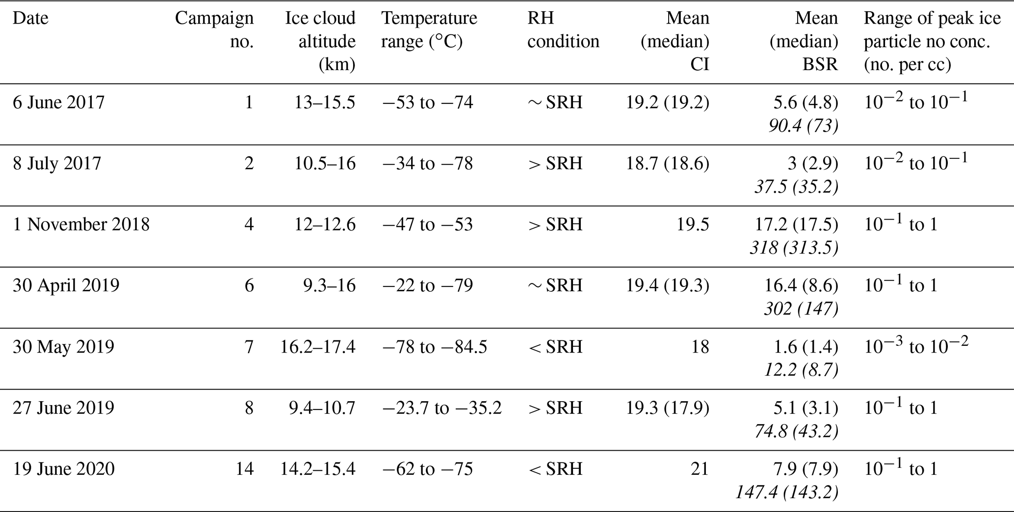
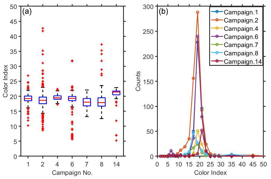
Figure 12 (a) Box plot of the colour index (CI) observed for the ice clouds found in different campaigns. The horizontal line in the centre of the box represents the median. The upper and lower edges of the box represent the third quartile (Q3) and first quartile (Q1), respectively. Similarly, the upper and lower whiskers represent $Q\mathrm{3}+\mathrm{1.5}\times (Q\mathrm{3}-Q\mathrm{1})$ and $Q\mathrm{1}-\mathrm{1.5}\times (Q\mathrm{3}-Q\mathrm{1})$, respectively. The data points beyond the whiskers (outliers) are shown with red star symbols. (b) The histogram of the CI values from each campaign. Different colours indicate the data from different campaigns.

Table 3 shows the mean (and median) values of CI and other parameters corresponding to the ice cloud layers from seven launches. Figure 12a shows the complete statistics of CI in the form of a box plot for the same ice cloud layers. Figure 12b shows a histogram of CI from each campaign indicated by different colours. In Table 3, ice clouds are seen above 9 km with temperatures colder than −20 ^∘C. For example, an ice cloud layer was found between 9.3 to 16 km on 30 April 2019 with temperatures in the range of −22 to −79 ^∘C, RH close to SRH, and mean (median) value of CI of 19.4 (19.3), where BSR is 16.4 (8.6) at 455 nm and 302 (147) at 940 nm and peak droplet concentration is in the range 10⁻¹ to 1 per cc. Similarly, from Table 3 the range of mean (median) values of BSR can be seen to be from 1.6 (1.4) to 17.2 (17.5) and 12.2 (8.7) to 318 (313) at 455 and 940 nm, respectively. Therefore, it is difficult to arrive at threshold values of BSR for ice clouds based on Table 3. This may be partly because BSR depends on not only the particle number concentration but also the size. However, it is interesting to note (except for a few cases in Table 3) that BSR data of ice clouds (at both channels) tend to be more abundant for densely populated clouds. On the other hand, the difference between mean and median values of CI is not large, and thus there is not much variance in CI within the ice cloud. It is also clear from Table 3 and Fig. 12a that about 90 %–95 % of CI values of ice clouds are above 15 and below 25 with mean and median values in the range of 18–20. The same is also seen in the histogram of CI shown (Fig. 12b) in different colours for different sounding dates where a greater number of points in a sounding are close to 20. Therefore, it may be concluded that the mean value of CI for ice clouds would be between 18 and 20.

The data from eight soundings are also analysed for CI (and other parameters) of liquid clouds. However, it is noted that liquid clouds were not observed as often as ice clouds in the balloon data. In the second campaign (8 July 2017), a liquid cloud layer was observed at altitudes from 4.7 to 4.86 km (160 m) with RH > SRH and temperatures in the range of −0.4 to −1.65 ^∘C. The mean value of CI corresponding to this liquid cloud layer is very high (around 50). Similarly, another liquid cloud layer was observed in the fourth campaign (1 November 2018) in the altitude range of 2–2.3 km (300 m). The corresponding CI values are high and above 100 (up to 200). A couple of thin supercooled liquid cloud layers were also identified on the same sounding between 6.1 and 6.17 km (7 m) and 6.6 and 6.8 km (200 m). The corresponding CI values are found with mean (median) values of 19.5 (19.4) and 32.6 (32.8), respectively. Apart from this, a strong boundary layer (liquid) cloud layer was observed on 23 March 2019 (fifth campaign) between 0.9 and 1.2 km (300 m). The corresponding CI of liquid cloud was found to be high with mean and median values of 60–80. From the above discussion (including the liquid cloud cases not discussed above), it is noticed that the CI for liquid clouds is high. The difference in CI values of liquid clouds can be attributed to the thickness of the cloud and the density and droplet size of liquid clouds.

Table 4 Colour index (CI) and backscatter ratio (BSR) of non-spherical (coarse) particle layers as identified by a CPS sonde. The BSR in the roman (italic) font is for 450 nm (940 nm). Bold (underlined) font values are observed in the monsoon (pre-monsoon) months.

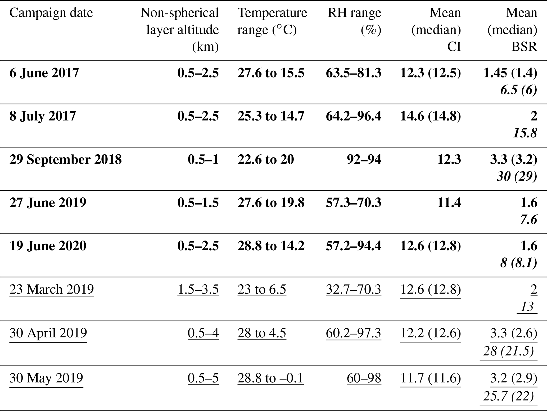
Non-spherical large dust aerosol particles were identified by DOP values from CPS in the lower troposphere where RH is far less than 100 %. Statistics on COBALD CI (and other parameters) for these non-spherical particle cases are presented in Table 4 using the data from eight soundings. For example, a non-spherical particle layer was found between 0.5 and 2.5 km in altitude on 6 June 2017 with temperatures in the range of 15.5 to 27.6 ^∘C and relative humidity being relatively dry, i.e. from 63.5 % to 81.3 %. The mean (median) value of CI corresponding to this non-spherical particle layer is 12.3 (12.5), BSR is 1.45 (1.4) at 455 nm and 6.5 (6) at 940 nm, and peak particle concentration is between 10⁻³ and 10⁻¹ cm⁻³. The peak particle concentration of all non-spherical layers is found to be in the same range and is hence not shown. From Table 4, it can be noticed that the non-spherical particle (aerosol) layer is found from near the surface to a 5 km altitude depending on the month or season. During the monsoon season (bold font in Table 4), non-spherical particle layers were observed mostly from near the surface (0.5 km) to 2.5 km, whereas during the pre-monsoon (underlined information) period it is found from 0.5 up to 5 km. The reason for the difference in layer thickness among seasons may be attributed to the mixing within the lower troposphere, long-range transport, and local sources. Since these layers are confined mostly to the lower troposphere, the temperatures are in a range from 27 to below 0 ^∘C. From the above statistics (pre-monsoon and monsoon cases) it may be stated that the mean and median values of CI for the non-spherical particle layer are distributed between 11 and 15 (irrespective of environmental humidity and season). BSR values for the non-spherical layer are between 1.4 and 3.5 at 455 nm, whereas there is little spread in the red channel.

3.4 Illustration of the aerosol–cloud relationship

In this section, an attempt is made to demonstrate the method to identify the relationship, if any, between aerosol and cloud properties observed using balloon observations of the BACIS campaigns. In the present analysis, we have restricted ourselves to only liquid or low-level clouds because aerosol interactions in these cloud categories are well established (Albrecht, 1989; Twomey, 1977).

The scheme (discussed in Sect. 2) is applied to the 15 balloon soundings of the BACIS campaigns, and six launches have been observed with low-level cloud and aerosol layers. Further, a scatter plot between logarithm values of the median cloud particle count of the cloud layer and a logarithm of median values of aerosol (blue) backscatter below cloud base (for 300, 400 and 500 m) is plotted in Fig. 13. A linear fit (line) of log–log values is also shown separately for all depths. It is noticed for depths 100 and 200 m below the cloud base that the relationship between aerosol and cloud cannot be discussed due to a lack of data points of aerosol backscatter ratio from individual campaigns. This could be the result of the elimination of the high values of COBALD particle backscatter (> 3.15) observed in this region (100 and 200 m below cloud base). In the cloud boundaries of about 100 and 200 m below the cloud base, an intermediate region exists where aerosol transformation to cloud particle and growth take place. Hence, it is tricky to perform the aerosol observation in this region. On the other hand, with similar elimination criteria (Sect. 2), aerosol backscatter could be obtained (from all five campaigns) for depths above 300 m (up to 500 m) from the cloud base. A good positive relationship is found between aerosol backscatter and cloud particle count, with a statistically significant Pearson correlation coefficient of about 0.9 and slope (ACI index) of 0.77 and 0.86 when the aerosol is considered from 300 and 400 m below the cloud base, respectively. For a depth of 500 m from the cloud base, the slope has decreased to 0.67 (correlation coefficient is also not significant with p-value > 0.05), indicating that aerosol influence weakens if the region below 400 m from the cloud base is considered. Therefore, it may be better to consider aerosols up to a depth of 400 m (below the cloud base) for understanding their influence on cloud properties. It is also emphasized that the slope (ACI index) value obtained in this analysis at all depths is well within the theoretical range of 0 to 1. However, with a greater number of balloon soundings it might be possible to have statistically significant aerosol data after constraining similar background and meteorological conditions to delineate their possible effects. Data obtained on 4 February 2020 were not considered in the analysis due to the high values of COBALD. The individual uncertainties in BSR_b and N_c were assumed to be 5 %, and the combined uncertainty in the ACI index is estimated as discussed in Sect. 2.4.7 (Eq. 7). It is found that the combined uncertainty in the estimated ACI index is found to be from 0.01 to 0.23 and 0.08 to 0.13, respectively, for particle backscatter data from 300 and 400 m below cloud base.

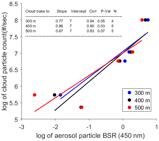
Figure 13 Scatter between logarithm values of COBALD median aerosol blue backscatter (x axis) from 300, 400, and 500 m below the cloud base and the corresponding CPS median cloud particle count (y axis) obtained from five balloon soundings with a linear fit (different coloured lines). The inset shows detailed statistics.

4 Summary

The BACIS (Balloon-borne Aerosol Cloud Interaction Studies) field campaigns have been conceptualized and successfully conducted using multiple instruments from Gadanki (13.45^∘ N, 79.2^∘ E), a location in southern India. Meteorological balloon payloads with a combination of lightweight and specialized sondes, such as COBALD and CPS, have been launched for the first time before a CALIPSO satellite overpass (close to Gadanki). Ground-based lidar (MPL, ceilometer, Mie lidar), and radar (MST radar and LAWP) were also operated during the campaign period. A total 15 balloon soundings have been conducted so far as part of the BACIS campaigns.

During the first two (pilot) campaigns, all essential ground-based and space-borne instruments were made available. Balloon-borne in situ measurements (CPS and COBALD) are assessed using the data from ground-based and space-borne remote sensing instruments (CALIPSO, MPL, and a Mie lidar) from two pilot campaigns (early hours of 6 June and 8 July 2017). The comparison shows reasonable agreement within in situ measurements and between ground-based and space-borne measurements and in situ measurements. It is observed that the in situ balloon soundings using a combination of specialized (COBALD and CPS) sondes adds to the cloud and aerosol information that can be obtained from an individual ground-based or space-borne instrument.

To discriminate aerosol from clouds in a profile, combined observations of COBALD and CPS from a campaign held on 27 June 2019 were inferred in detail. Using CPS data, liquid, supercooled, and ice clouds were identified. COBALD data of BSR corresponding to the ice clouds were found to be 1–10 (at the blue channel) and have a CI of 10 to 20. In addition to cloud features, CPS has also detected cloud particle layers at low altitudes (under dry conditions). These layers may be regarded as non-spherical (coarse-mode) aerosol particle layers because ice clouds (with non-spherical cloud particles) cannot exist at lower heights. An attempt is also made to infer the size of cloud particles using the CPS data of the intensity of scattered light (I₅₅) and the COBALD colour index. Based on CPS scattered light data, the liquid droplet size (for the above case) is estimated to be 2–14 µm, and for ice particles it is a combination of particles with sizes of 80–140 and 2–14 µm. The estimates of ice particle sizes using CI data from COBALD supported the size interpretations of ice particles by CPS.

Further, combined observations from COBALD and CPS (BSR, CI, and peak particle number concentration data based on information of the cloud phase) are analysed from multiple (eight) balloon soundings from BACIS campaigns. From these statistics, it is found that the mean value of the CI of ice clouds is found to be between 18 and 20. BSRs (at both wavelengths) have a wide range of values, and hence threshold values for ice clouds could not be arrived at. However, in some cases BSR increased with ice clouds of higher droplet number concentration. In the case of non-spherical particle (aerosol) layers (in the lower troposphere), the mean values of CI and BSR (at 455 nm) are found to be between 11 and 15 and 1.4 and 3.5, respectively. These non-spherical particle layers may correspond to coarse-mode (dust) aerosols (as discussed above).

The relationship between aerosol and cloud in low-level (liquid) clouds is illustrated using balloon data from BACIS campaigns. CPS cloud particle count and COBALD particle backscatter at the blue channel were considered to be cloud and aerosol proxies, respectively. A scheme is developed to carefully identify the cloud layers from CPS data and particle (aerosol) backscatter below the cloud from COBALD data (in a profile). However, the relationships were analysed separately using particle backscatter data from 100 to 500 m below the base height for the first cloud layer. The results show a statistically significant correlation of 0.9 and a slope (aerosol–cloud interaction index, ACI) of 0.7 (0.86) obtained between particle backscatter from 300 m (500 m) below the cloud base and the corresponding cloud particle count. The ACI index value obtained is well within the theoretical limits of 0 to 1, which is indicative of the aerosol activation process of the cloud. The uncertainty in the estimated value of the ACI index is 0.01 to 0.23 and 0.08 to 0.13, respectively, for backscatter data from 300 and 400 m below the cloud base.

Statistical estimates and threshold values of CI and BSR for cloud (liquid, supercooled, ice) and non-spherical particles attempted here will greatly help to separate a COBALD profile for aerosol and cloud. However, immediate efforts are needed to understand the portion of the COBALD profile with no cloud detection from CPS. This portion of the COBALD profile may correspond to either aerosol with fine-mode particles and/or a thin cloud not detectable by a CPS. On the other hand, estimates of size discussed here (from CPS and COBALD) are purely based on Mie theory and laboratory data. However, with assumptions of the log-normal distribution of particles and measurements from COBALD (BSR, CI), the theoretical estimate of the particle size distribution of aerosol and cloud is possible. It makes sense to cross-check rough estimates of size from a CPS with COBALD size distributions rather than using CI variations. It is also planned to add a size distribution measurement to the balloon payload for cross-verification and validation. Apart from this, in some of the cases we have noticed that the COBALD return signal is saturated for liquid and supercooled cloud in the presence of a thick liquid cloud. Hence, the information from a greater number of future launches will help to conclude the statistical figures and threshold values for liquid clouds, as well as other forms of clouds, to discriminate between aerosol and cloud in a profile and to better quantify the aerosol–cloud relationship. Further to this end, attempts will be made to quantify aerosol–cloud interactions (with the multi-instrument data), the role of vertical wind and turbulence in the aerosol–cloud interaction and ice cloud interactions, and so on. In a nutshell, the results presented in this study indeed demonstrate the potential of the observational approach to further the understanding of the aerosol–cloud process.