Turbulence parameters measured by the Beijing mesosphere–stratosphere–troposphere radar in the troposphere and lower stratosphere with three models: comparison and analyses

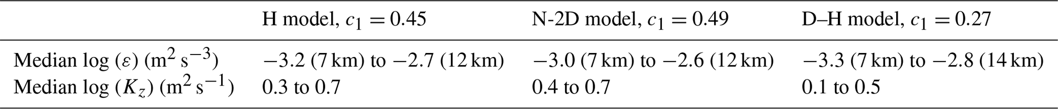
Based on the quality-controlled observational spectral width data of the Beijing mesosphere–stratosphere–troposphere (MST) radar in the altitudinal range of 3–19.8 km from 2012 to 2014, this paper analyses the relationship between the proportion of negative turbulent kinetic energy (N-TKE) and the horizontal wind speed and the vertical shear of horizontal wind domain and gives the distributional characteristics of atmospheric turbulence parameters obtained by using different calculation models. Three calculation models of the spectral width method were used in this study – namely the H model (Hocking, 1985), N-2D model (Nastrom, 1997) and D–H model (Dehghan and Hocking, 2011). The results showed that the proportion of N-TKE in the H model, N-2D model and D–H model increases with the horizontal wind speed u and/or the vertical shear of horizontal wind speed $\frac{\partial u}{\partial z}$, and the maximum values are 60 %, 45 % and 35 %, respectively. When the$\left|\frac{\partial u}{\partial z}\right|$ is greater than 0.006 s⁻¹, the N-TKE of the H model increases sharply with $\left|\frac{\partial u}{\partial z}\right|$; the increase rate is about $\frac{\mathrm{20}\mathit{\%}}{\mathrm{0.002}{\mathrm{s}}^{-\mathrm{1}}}$. For these three models, the results are similar except that the vertical shear of the horizontal wind speed is greater than 0.006 s⁻¹. When $\frac{\partial u}{\partial z}>\mathrm{0.006}$ s⁻¹, the proportion of N-TKE in the N-2D and H models increases with $\frac{\partial u}{\partial z}$, while the proportion in the D–H model is less than 10 % and has slight variation. However, it is still necessary to consider the applicability of the N-2D model and D–H model in some weather processes with strong winds. The distributional characteristics with height of the turbulent kinetic energy dissipation rate ε and the vertical eddy diffusion coefficient K_z derived by the three models are consistent with previous studies. Still, there are differences in the values of turbulence parameters. Also, the range resolution of the radar has little effect on the differences in the range of turbulence parameters' values. The median values of ε in the H model, N-2D model and D–H model is 10^−3.2–10^−2.7, 10^−3.0–10^−2.6 and 10^−3.3–10^−2.8 m² s⁻³, respectively. The median values of K_z in these three models are 10^0.3–10^0.7, 10^0.4–10^0.7 and 10^0.1–10^0.5 m² s⁻¹.

1 Introduction

Small-scale turbulence plays a vital role in the vertical exchange of heat, momentum and mass in the atmosphere. Originally, observing turbulence in the free atmosphere was mainly carried out by sounding balloons and aircraft (e.g. Lilly et al., 1974). However, with the development of atmospheric radar, it has since become possible to quantitatively calculate turbulence parameters (e.g. the vertical eddy diffusion coefficient K_z and turbulence energy dissipation rate ε) in the free atmosphere through remote sensing (Weinstock, 1981; Hocking, 1983).

Most research on turbulence parameters using atmospheric radar is based on the Kolmogorov hypothesis of isotropic turbulence at the inertial sub-region scale (Batchelor, 1953; Tatarski, 1961, 1971). To detect atmospheric turbulence intensity by atmospheric radar, the radar echo signal should come from turbulence scattering. In fact, at some heights, such as near the tropopause region, the scattering echo can be affected by specular reflection. However, the influence of specular reflection is weaker for inclined beams than for vertical beam. Therefore, it is more appropriate to use the observational data of inclined beams for analysis. The Doppler spectrum width measured by radar contains atmospheric turbulence intensity information, and the turbulence is on a smaller scale than the radar sampling volume.

The mesosphere–stratosphere–troposphere (MST) radar is a unique and essential means to detect turbulence characteristics in multiple layers of the atmosphere. As a kind of atmospheric radar, MST radar is based on the scattering effect of atmospheric refraction irregularities on the electromagnetic waves emitted by the radar to carry out remote sensing detection of the atmosphere. Therefore, the radar echo contains atmospheric turbulence information (such as echo power and spectral width). Also, the scale of the detection target is in the inertial sub-region. For the current detection methods, MST radar is an indispensable instrument to detect the troposphere, stratosphere and mesosphere. The macroscopic characteristic parameters (ε, K_z) used to describe atmospheric turbulence are calculated using MST radar data with high spatial and temporal resolution. At present, three methods are mainly used: the power method (Hocking, 1985), the Doppler spectral width method (Hocking, 1985; Nastrom, 1997; Dehghan and Hocking, 2011; Fukao et al., 2014) and the vertical velocity variance method (Satheesan and Murthy, 2002).

The basic idea of the power method is that the radar echo power can be used to estimate the structure constant of the atmospheric refractive index $C_n^{\mathrm{2}}$ (Rao et al., 2001a), and the mathematical relationship between $C_n^{\mathrm{2}}$ and ε can be determined by the outer scale of turbulence. Therefore, the turbulence parameters ε and K_z can be calculated by the radar echo power. ε has a mathematical relationship with the variance of vertical velocity ($\stackrel{\mathrm{‾}}{{\mathit{\omega }}^{\mathrm{2}}}$): $\mathit{\epsilon }=\frac{\mathrm{6.1}F\stackrel{\mathrm{‾}}{{\mathit{\omega }}^{\mathrm{2}}}N}{\mathrm{2}\mathit{\pi }}=\mathrm{0.97}\stackrel{\mathrm{‾}}{{\mathit{\omega }}^{\mathrm{2}}}N$, where F is the fraction of the measured velocity variance (of wind velocity spectrum) that resides in the inertial subrange and the rest in the buoyancy subrange, and N is the Brunt–Väisälä (B–V) frequency. Satheesan and Murthy (2002) have taken F=1. The power method requires temperature, atmospheric pressure, and water vapour profile data, as well as the assumption that the radar absolute calibration and radar detection volume are filled with turbulence. The vertical velocity law requires precise vertical velocity. For vertical beams, due to the interference of non-turbulent signals, the accuracy of vertical velocity needs to be improved. Delage et al. (1997) compared the statistical characteristics of ε with the power method and the spectral width method, separately. The results showed that the results of the two methods are in good agreement when the turbulent layer is thinner than 600 m.

For the spectral width method, the conditions of the above two methods are not necessary. Radar echo is the backscattering result of all scattering cells in the radar sampling space. For a given range library, due to coherent integration and incoherent integration of the radar, the random motion of the scattering cells is shown as the random distribution of its Doppler velocity near the mean wind speed. That is, the Doppler spectrum of the radar is broadened. The Doppler spectral width contains atmospheric turbulence information and can be used to calculate the macro parameters of turbulence.

The present study shows that the spectrum width σ_o in the radar power spectrum has a turbulent contribution σ_t and non-turbulent contribution σ_u, such as beam broadening σ_b and shear broadening σ_s, under the condition of no interference signal:

$$\begin{array}{}\text{(1)}& {\mathit{\sigma }}_{\mathrm{o}}^{\mathrm{2}}={\mathit{\sigma }}_{\mathrm{t}}^{\mathrm{2}}+{\mathit{\sigma }}_{\mathrm{u}}^{\mathrm{2}}={\mathit{\sigma }}_t^{\mathrm{2}}+{\mathit{\sigma }}_{\mathrm{s}}^{\mathrm{2}}+{\mathit{\sigma }}_{\mathrm{b}}^{\mathrm{2}}+{\mathit{\sigma }}^{\mathrm{2}},\end{array}$$

where σ² refers to the influence of other factors, such as gravity waves, which will also cause the spectral width to increase in the total acquisition time of the radar. However, the contribution of σ² is relatively small in the region below 20 km, where ${\mathit{\sigma }}_{\mathrm{s}}^{\mathrm{2}}+{\mathit{\sigma }}_{\mathrm{b}}^{\mathrm{2}}$ can be combined into a term ${\mathit{\sigma }}_{\mathrm{s}\mathrm{\&}\mathrm{b}}^{\mathrm{2}}$, which represents beam and shear effects (Nastrom, 1997).

In current studies, there are mainly three models used to calculate non-turbulent spectral width: Hocking (1983, 1985) proposed an empirical model (called the H model), Nastrom (1997) put forward a calculation model and revealed that their 2D model could meet the estimation requirements (called the N-2D model), and Dehghan and Hocking (2011) made a further derivation of the N-2D model and thus developed a new calculation model (called the D–H model). The three models are described in detail in Sect. 2.3.

Due to the differences in the calculation models of turbulence spectral width, the specific equations for calculating turbulence parameters using the spectral width method are different, but they have similar expressions. The relation between the turbulent energy dissipation rate ε and ${\mathit{\sigma }}_{\mathrm{t}}^{\mathrm{2}}$ is as follows (Hocking, 1983; Weinstock, 1981):

$$\begin{array}{}\text{(2)}& \mathit{\epsilon }=c_{\mathrm{1}}{\mathit{\sigma }}_{\mathrm{t}}^{\mathrm{2}}N,\end{array}$$

where c₁ is a constant and N is the B–V frequency (s⁻¹). For the H model, c₁ varies in different studies, generally ranging from 0.45 to 0.5 (e.g. Hocking, 1999; Wilson, 2004). Hocking et al. (2016) suggested that 0.5 ± 0.25 was a reasonable range for c₁. For the H model, this paper takes c₁=0.45, and Hocking (1999) obtains it from experience (Kohma et al., 2019). For the N-2D model, the turbulence in the inertial subregion is assumed to be isotropic. For a stably stratified atmosphere, ${\mathit{\sigma }}_{\mathrm{t}}^{\mathrm{2}}$ has the following relationship with ε (Weinstock, 1981; Nastrom and Eaton, 1997): $\mathit{\epsilon }=A^{-\frac{\mathrm{3}}{\mathrm{2}}}N{\mathit{\sigma }}_{\mathrm{t}}^{\mathrm{2}}$, where A is the Kolmogorov constant, taking A=1.6 and c₁≈0.49. For the D–H model, this paper takes c₁=0.27 (Dehghan and Hocking, 2011). That is, several studies pointed out that the velocity variance measured by the radar is related to the transverse one-dimensional spectrum function for the direction radial from the radar (Dehghan and Hocking, 2011; Hocking, 1999). $N^{\mathrm{2}}=g\frac{\mathrm{d}\ln \left(\mathit{\theta }\right)}{\mathrm{d}z}$, and the potential temperature θ can be calculated by the equation $\mathit{\theta }=T{\left(\frac{\mathrm{1000}}{P}\right)}^{\mathrm{0.286}}$, where T is the temperature (K) and P is atmospheric pressure (hPa). θ can be calculated from the radiosonde data.

K_z is closely related to ε (Fukao et al., 1994; Nastrom and Eaton, 1997; Rao et al., 2001b). The equation is as follows:

$$\begin{array}{}\text{(3)}& K_z=c_{\mathrm{2}}\mathit{\epsilon }{N}^{-\mathrm{2}}=c_{\mathrm{1}}{c}_{\mathrm{2}}{N}^{-\mathrm{1}}{\mathit{\sigma }}_{\mathrm{t}}^{\mathrm{2}},\end{array}$$

where ε is the dissipation rate of turbulent energy, N is the B–V frequency and c₂ is a constant. In this paper, c₂=0.3 (Fukao et al., 1994).

When the spectral width method is used to calculate the turbulence parameters, there is a negative value of ${\mathit{\sigma }}_{\mathrm{t}}^{\mathrm{2}}$ in the results of the H, N-2D and D–H models, resulting in negative values of the turbulence parameters ε and K_z – that is, negative turbulent kinetic energy (N-TKE). Dehghan and Hocking (2011) believed that the factors that cause the negative value of the turbulent spectrum width mainly include the non-isotropy of the scatterer (relatively small contribution), the influence of the uncertainty of the calculation of the observed spectrum width and the spectrum width broadening term (Eq. 1). The ${\mathit{\sigma }}_{\mathrm{o}}^{\mathrm{2}}$ is related to the calculation method of each moment of the power spectrum and the resolution of the power spectrum (depends on the data length, s), while ${\mathit{\sigma }}_{\mathrm{s}\mathrm{\&}\mathrm{b}}^{\mathrm{2}}$ depends on the uncertainty of the calculation of horizontal wind speed. When the ${\mathit{\sigma }}_{\mathrm{o}}^{\mathrm{2}}$ value is low and the ${\mathit{\sigma }}_{\mathrm{s}\mathrm{\&}\mathrm{b}}^{\mathrm{2}}$ value is high, ${\mathit{\sigma }}_{\mathrm{t}}^{\mathrm{2}}$ will be low, sometimes even negative, and when ${\mathit{\sigma }}_{\mathrm{o}}^{\mathrm{2}}$ is high and ${\mathit{\sigma }}_{\mathrm{s}\mathrm{\&}\mathrm{b}}^{\mathrm{2}}$ is low, ${\mathit{\sigma }}_{\mathrm{t}}^{\mathrm{2}}$ will be high. Kohma et al. (2019) pointed out that the median of ε differs slightly (<3 %) between including and excluding negative numbers.

Since the influence of non-isotropy is relatively small, for a radar (assuming constant radar parameters), Eq. (1) can be simplified as ${\mathit{\sigma }}_{\mathrm{o}}^{\mathrm{2}}={\mathit{\sigma }}_{\mathrm{t}}^{\mathrm{2}}+{\mathit{\sigma }}_{\mathrm{s}\mathrm{\&}\mathrm{b}}^{\mathrm{2}}$ in the tropospheric and lower stratospheric range. The main factor causing ${\mathit{\sigma }}_{\mathrm{t}}^{\mathrm{2}}<$ is the calculation accuracy of ${\mathit{\sigma }}_{\mathrm{s}\mathrm{\&}\mathrm{b}}^{\mathrm{2}}$. If the radar parameter is constant, the factors affecting the calculation accuracy of ${\mathit{\sigma }}_{\mathrm{s}\mathrm{\&}\mathrm{b}}^{\mathrm{2}}$ are not only the accuracy of the calculation of the horizontal wind field (the horizontal wind speed and the vertical shear of horizontal wind), but also the applicability of the calculation model itself may be different under different horizontal wind field conditions. For example, Dehghan and Hocking (2011) believed that in some strong wind shear conditions, a more universal model than the D–H model is needed. When the probability of N-TKE is high, the applicability of the model is the main factor affecting the calculation accuracy of ${\mathit{\sigma }}_{\mathrm{s}\mathrm{\&}\mathrm{b}}^{\mathrm{2}}$. Moreover, when the amount of data involved is statistically too small, the credibility of the final turbulence parameter structure will be reduced. Therefore, before analysing the turbulence parameters, the applicability of the non-turbulent spectral width calculation model in different horizontal wind fields should be analysed.

Based on 3 years of observational data from the Beijing MST radar (2012, 2013 and 2014), this paper uses three models to calculate the non-turbulent spectrum width and analyses the distributional characteristics of the N-TKE ratio under different horizontal wind speeds and horizontal wind vertical shear conditions. It can also be understood as the frequency distribution characteristics of horizontal wind speed and vertical shear of horizontal wind speed when N-TKE appears. Furthermore, the vertical distribution characteristics of the turbulence parameters are analysed, and the applicability of the three models is given. By studying the applicability of the calculation models in the different wind field conditions, the appropriate model can be selected to calculate the non-turbulent spectrum width to improve the reliability of the calculation results of turbulence parameters.

This remainder of the paper is structured as follows: Sect. 2 describes the data and methods, in which the three models used to calculate non-turbulent broadening are outlined. In Sect. 3, the relationship between the occurrence probability of N-TKE and horizontal wind speed as well as vertical shear of horizontal wind speed along with the analysis results of the distributional characteristics of turbulence parameters are given. Sections 4 and 5 are the discussion and conclusion, respectively.

2 Data and methods

2.1 Beijing MST radar observations

The data used in this paper are the observational data of the Beijing MST radar, which is located at the Xianghe Observatory of the Whole Atmosphere, Institute of Atmospheric Physics, Chinese Academy of Sciences (39.78^∘ N, 116.95^∘ E). The Beijing MST radar is a five-beam (east–west, north–south and vertical) clear air turbulence (CAT) detection pulse Doppler radar, which was built and put into service in 2011 and has accumulated a long period of data. According to analyses of the reliability and accuracy of the Beijing MST radar data (Tian and Lü, 2016, 2017), it has good detection capability in the troposphere, lower stratosphere and mesosphere to lower thermosphere. Tian and Lü (2017) and Tian et al. (2021) described the Beijing MST radar in more detail. The parameters of the Beijing MST radar are shown in Table 1. In middle mode, it takes about 5 min for five beams to complete one data acquisition.

Table 1 Parameters of the Beijing MST radar.

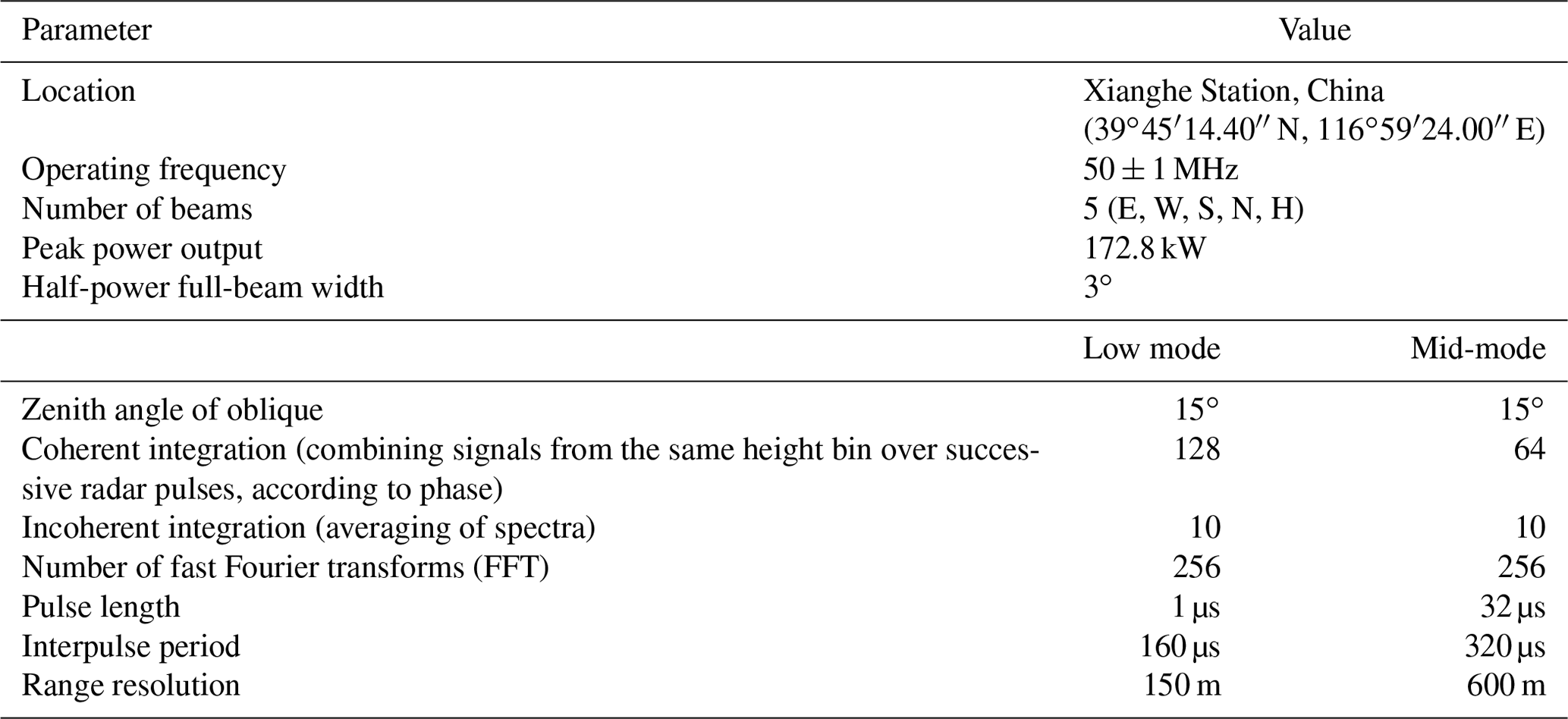
This paper uses data from four oblique beams (east–west, north–south) with a zenith angle of 15^∘. The radial range resolutions of mid-mode and low-mode observations are 600 and 150 m, respectively. The advantage of using vertical beam detection results to calculate turbulence parameters is that the influence of wind shear does not need to be considered (Kantha et al., 2017). However, the vertical beam is more susceptible to specular reflection, especially in the tropopause region, where the echo signal spectrum is narrow and unrelated to turbulence (e.g. Fukao et al., 1994; Tsuda et al., 1986; Birner, 2006), which is based on isotropic scattering. The spectral width method is based on the isotropic scattering, which has the hypothesis that the radial wind speed variance (Doppler spectral width) detected by the radar is equal to the turbulence intensity. At the same time, because the radial velocity of the vertical beam is small, it is more affected by ground clutter near zero frequency, which reduces the accuracy of vertical beam spectrum observations. Compared with the vertical beam, the oblique beam is less likely to be affected by specular reflection than by isotropic scattering due to isotropic turbulence (Fukao et al., 1994; Tsuda et al., 1986). Therefore, based on the above considerations, this paper uses the spectral width data obtained from the four oblique beams to calculate the turbulence parameters. In this paper, the improved power spectral density processing algorithm of Chen et al. (2020) is applied to suppress non-atmospheric signals and obtain reliable spectral width data effectively.

2.2 Radiosonde data

For the spectral width method, N² profiles need to be provided in other ways when turbulence parameters are calculated by the turbulent spectral width. In this paper, the temperature profile data of the Beijing conventional radiosonde (54511, 39.8^∘ N, 116.4^∘ E) are used to calculate N². The straight-line distance between the MST radar and the radiosonde launch site is about 40 km. Conventional radiosonde probes are operated twice a day (11:15 and 23:15 UTC) and recorded every 1–2 s, with a vertical resolution of about 10 m. In this paper, the observational data of the mid-mode (11:10, 11:40, 23:10 and 23:40 UTC) and low mode (11:05, 11:35, 23:05 and 23:35 UTC) of the Beijing MST radar from 2012 to 2014, corresponding to the radiosonde, are selected to calculate the turbulence parameters. The number of radiosonde profiles involved in the calculation of both the mid-mode and low mode is 3532. The radiosonde data are interpolated with a resolution of 600 m in the radar mid-mode to facilitate the calculation. In low observation mode, the radiosonde data are interpolated with a resolution of 150 m.

2.3 Methods used to estimate turbulence parameters

In the troposphere–lower stratosphere region, time broadening (also called the gravity wave term) has a relatively small effect on the observed spectrum width (Nastrom, 1997). The broadening of the spectrum caused by turbulence mainly considers shear and beam broadening: ${\mathit{\sigma }}_{\mathrm{t}}^{\mathrm{2}}={\mathit{\sigma }}_{\mathrm{o}}^{\mathrm{2}}-{\mathit{\sigma }}_{\mathrm{s}}^{\mathrm{2}}-{\mathit{\sigma }}_{\mathrm{b}}^{\mathrm{2}}$. After calculating the radar observation spectrum width, we then estimate ${\mathit{\sigma }}_{\mathrm{s}}^{\mathrm{2}}$ and ${\mathit{\sigma }}_{\mathrm{b}}^{\mathrm{2}}$ to obtain ${\mathit{\sigma }}_{\mathrm{t}}^{\mathrm{2}}$. The atmospheric turbulence parameters (ε, K_z) can be estimated by ${\mathit{\sigma }}_{\mathrm{t}}^{\mathrm{2}}$ according to Eqs. (2) and (3). Based on this, there are currently several calculation models for calculating ${\mathit{\sigma }}_{\mathrm{t}}^{\mathrm{2}}$ by the spectral width method, and they have similar expressions.

Before introducing the three calculation models, due to the differences in expression between the models, it is necessary to understand the relationship between the power spectrum half-power half-width (σ_½) and the Doppler spectrum width (σ), $\mathit{\sigma }=\frac{{\mathit{\sigma }}_{\frac{\mathrm{1}}{\mathrm{2}}}}{\sqrt{\mathrm{2}\ln \mathrm{2}}}$. The units of σ and σ_½ can be Hz or m s⁻¹. The relationship between the Doppler velocity v and the Doppler frequency shift f is as follows: $v=f\cdot \mathit{\lambda }/\mathrm{2}$, where λ is the wavelength of the electromagnetic wave emitted by the radar. The Doppler velocity spectrum width σ_v (or the radial velocity standard deviation) and the Doppler frequency spectrum width σ_f have the following relationship: ${\mathit{\sigma }}_{\mathrm{v}}=\frac{\mathit{\lambda }}{\mathrm{2}}{\mathit{\sigma }}_{\mathrm{f}}$. Similarly, ${\mathit{\sigma }}_{\mathrm{v}\frac{\mathrm{1}}{\mathrm{2}}}=\frac{\mathit{\lambda }}{\mathrm{2}}{\mathit{\sigma }}_{\mathrm{f}\frac{\mathrm{1}}{\mathrm{2}}}$, where σ_v½ and σ_f½ are the Doppler velocity and half-power half-width (Hz), respectively.

2.3.1 H-model

According to Hocking (1985), the beam broadening can be estimated using the following equation:

$$\begin{array}{}\text{(4)}& \begin{array}{rl}{\mathit{\sigma }}_{\mathrm{vb}}& ={\mathit{\sigma }}_{\mathrm{f}\frac{\mathrm{1}}{\mathrm{2}}b}\cdot {\displaystyle \frac{\mathit{\lambda }}{\mathrm{2}}}/\left(\sqrt{\mathrm{2}}\ln \mathrm{2}\right)\\ & =\left(\mathrm{1.0}\right)\cdot {\displaystyle \frac{\mathrm{2}}{\mathit{\lambda }}}\cdot {\mathit{\theta }}_{\mathrm{1}/\mathrm{2}}^{\left(\mathrm{2}\right)}\cdot u\cdot {\displaystyle \frac{\frac{\mathit{\lambda }}{\mathrm{2}}}{\sqrt{\mathrm{2}\ln \mathrm{2}}}}\\ & =\left(\mathrm{1.0}\right)\cdot {\displaystyle \frac{{\mathit{\theta }}_{\mathrm{1}/\mathrm{2}}^{\left(\mathrm{2}\right)}\cdot u}{\sqrt{\mathrm{2}\ln \mathrm{2}}}},\end{array}\end{array}$$

where σ_vb is the Doppler velocity spectrum width caused by the beam (m s⁻¹); σ_f½b is the half-power half-width (Hz) of the Doppler frequency caused by the beam; ${\mathit{\sigma }}_{\mathrm{f}\frac{\mathrm{1}}{\mathrm{2}}\mathrm{b}}=\left(\mathrm{1.0}\right)\times \frac{\mathrm{2}}{\mathit{\lambda }}{\mathit{\theta }}_{\mathrm{1}/\mathrm{2}}^{\left(\mathrm{2}\right)}V$, where λ is the wavelength of the electromagnetic wave emitted by the radar (the λ of the Beijing MST radar is 6 m); and ${\mathit{\theta }}_{\mathrm{1}/\mathrm{2}}^{\left(\mathrm{2}\right)}$ is the two-way (transmit and receive) half-power half-width in the polar coordinate system (Hocking et al., 2016, Eq. 7.34). The ${\mathit{\theta }}_{\mathrm{1}/\mathrm{2}}^{\left(\mathrm{1}\right)}$ of the Beijing MST radar is $\frac{\mathrm{1.5}}{\mathrm{180}}\times \mathit{\pi }$ (radians), ${\mathit{\theta }}_{\mathrm{1}/\mathrm{2}}^{\left(\mathrm{1}\right)}=\sqrt{\mathrm{2}}{\mathit{\theta }}_{\mathrm{1}/\mathrm{2}}^{\left(\mathrm{2}\right)}$. And u is the average horizontal wind speed (m s⁻¹) calculated by the oblique the beam.

Wind shear broadening can be calculated with the following equation (Hocking, 1985; Fukao et al., 2014):

$$\begin{array}{}\text{(5)}& {\mathit{\sigma }}_{\mathrm{vs}}={\displaystyle \frac{{\mathit{\sigma }}_{\mathrm{v}\frac{\mathrm{1}}{\mathrm{2}}\mathrm{s}}}{\sqrt{\mathrm{2}\ln \mathrm{2}}}}={\displaystyle \frac{\mathrm{1}}{\mathrm{2}}}\cdot {\displaystyle \frac{\left|\frac{\partial u}{\partial z}\right|\sin \left(\mathit{\chi }\right)\mathrm{\Delta }r}{\sqrt{\mathrm{2}\ln \mathrm{2}}}},\end{array}$$

where σ_vs is the widening of the Doppler velocity spectrum caused by the vertical shear of the horizontal wind, and σ_v½s is the half-power half-width (m s⁻¹) caused by the horizontal wind shear. ${\mathit{\sigma }}_{\mathrm{v}\frac{\mathrm{1}}{\mathrm{2}}\mathrm{s}}=\frac{\mathrm{1}}{\mathrm{2}}\cdot \left|\frac{\partial u}{\partial z}\right|\sin \left(\mathit{\chi }\right)\mathrm{\Delta }r$, where $\left|\frac{\partial u}{\partial z}\right|$ is the vertical shear of horizontal wind, χ is the zenith angle of the beam and Δr is radial resolution of the radar.

In fact, only the beam direction component of the horizontal wind vector contributes to the broadening of the radar spectrum. So the correct value of wind shear should be ${\frac{\partial u}{\partial z}}_{\mathit{\varphi }}$, where φ is the azimuth direction of the mean wind (Nastrom, 1997; Dehgan and Hocking, 2011). In this study, we take the zonal (meridional) winds to explore the shear broadening effects of the east-and-west (north and south) beam. The vertical shear of horizontal wind $\frac{\partial u}{\partial z}$ is as follows:

• for the east and west beams

  $$\begin{array}{}\text{(6)}& u=u_x,{\displaystyle \frac{\partial u}{\partial z}}={\displaystyle \frac{\partial u_x}{\partial z}}\end{array}$$

• and for the north and south beams

  $$\begin{array}{}\text{(7)}& u=v_y,{\displaystyle \frac{\partial u}{\partial z}}={\displaystyle \frac{\partial v_y}{\partial z}},\end{array}$$

where u_x and v_y are zonal and meridional wind, respectively. The directions of u_x and v_y have no effect on the results of H model and have very little effect on the D–H model and N-2D model. This study used the absolute value of the component of the horizontal wind vector and did not overdiscuss the effect of wind direction, where $\frac{\partial u}{\partial z}$ contains positive and negative values.

In this paper, Eqs. (4) and (5) are referred to as the H model for short. For the vertical beam (χ=0^∘), the value of the broadening term caused by wind shear is zero, so Eq. (4) can be used to calculate the ${\mathit{\sigma }}_{\mathrm{s}\mathrm{\&}\mathrm{b}}^{\mathrm{2}}$ of the vertical beam. The effect of beam broadening can be processed before obtaining the power spectrum. For example, the PANSY radar uses irregular antennas, and deconvolution is performed before the power spectrum is obtained. Therefore, when using radar data to calculate turbulence parameters, there is no need to consider beam broadening (Fukao et al., 2014; Kohma et al., 2019).

Incorporating Eqs. (4) and (5) into the equation ${\mathit{\sigma }}_{\mathrm{t}}^{\mathrm{2}}={\mathit{\sigma }}_{\mathrm{o}}^{\mathrm{2}}-{\mathit{\sigma }}_{\mathrm{s}}^{\mathrm{2}}-{\mathit{\sigma }}_{\mathrm{b}}^{\mathrm{2}}$ allows ${\mathit{\sigma }}_{\mathrm{t}}^{\mathrm{2}}$ to be calculated. Since the turbulence in the inertial subregion satisfies the hypothesis of specific isotropy, the variance $\stackrel{\mathrm{‾}}{v^{\mathrm{2}}}$ (or turbulent energy) of the scatterer's wind speed fluctuation and the turbulence spectrum width ${\mathit{\sigma }}_{\mathrm{t}}^{\mathrm{2}}$ have the following relationship:

$$\begin{array}{}\text{(8)}& \begin{array}{rl}\stackrel{\mathrm{‾}}{v^{\mathrm{2}}}={\mathit{\sigma }}_{\mathrm{t}}^{\mathrm{2}}& ={\mathit{\sigma }}_{\mathrm{vo}}^{\mathrm{2}}-{\left(\left(\mathrm{1.0}\right)\cdot {\displaystyle \frac{{\mathit{\theta }}_{\mathrm{1}/\mathrm{2}}^{\left(\mathrm{2}\right)}\cdot u}{\sqrt{\mathrm{2}\ln \mathrm{2}}}}\right)}^{\mathrm{2}}\\ & -{\left({\displaystyle \frac{\mathrm{1}}{\mathrm{2}}}\cdot \left|{\displaystyle \frac{\partial u}{\partial z}}\right|{\displaystyle \frac{\sin \left(\mathit{\chi }\right)\mathrm{\Delta }r}{\sqrt{\mathrm{2}\ln \mathrm{2}}}}\right)}^{\mathrm{2}},\end{array}\end{array}$$

where σ_vo is the observed Doppler velocity spectrum width (m s⁻¹) and σ_vo can be calculated by Gaussian fitting.

2.3.2 N-2D model

Nastrom (1997) and others believe that their two-dimensional model can describe the broadening of the spectral width caused by the beam and horizontal wind shear well (referred to as the N-2D model). The N-2D model considers the effects of beam and shear at the same time. That is, ${\mathit{\sigma }}_{\mathrm{s}}^{\mathrm{2}}$ and ${\mathit{\sigma }}_{\mathrm{b}}^{\mathrm{2}}$ in Eq. (1) are combined into a term ${\mathit{\sigma }}_{\mathrm{s}\mathrm{\&}\mathrm{b}}^{\mathrm{2}}$. The equation for broadening the spectral width is as follows:

$$\begin{array}{}\text{(9)}& \begin{array}{rl}{\mathit{\sigma }}_{\mathrm{s}\mathrm{\&}\mathrm{b}}^{\mathrm{2}}& ={\displaystyle \frac{{\mathit{\theta }}_{\mathrm{1}/\mathrm{2}}^{(\mathrm{1}{)}^{\mathrm{2}}}}{\mathrm{3}}}{u}^{\mathrm{2}}{\cos }^{\mathrm{2}}\mathit{\chi }-{\displaystyle \frac{\mathrm{2}{\mathit{\theta }}_{\mathrm{1}/\mathrm{2}}^{(\mathrm{1}{)}^{\mathrm{2}}}}{\mathrm{3}}}{\sin }^{\mathrm{2}}\mathit{\chi }\left(u{\displaystyle \frac{\partial u}{\partial z}}r\cos \mathit{\chi }\right)\\ & +{\mathit{\theta }}_{\mathrm{1}/\mathrm{2}}^{(\mathrm{1}{)}^{\mathrm{2}}}/\mathrm{24}\left(\mathrm{3}+\cos \mathrm{4}\mathit{\chi }-\mathrm{4}\cos \mathrm{2}\mathit{\chi }\right){\left({\displaystyle \frac{\partial u}{\partial z}}\right)}^{\mathrm{2}}{r}^{\mathrm{2}}\\ & +\left({\displaystyle \frac{{\mathit{\theta }}_{\mathrm{1}/\mathrm{2}}^{(\mathrm{1}{)}^{\mathrm{2}}}}{\mathrm{3}}}\cos \mathrm{4}\mathit{\chi }+{\sin }^{\mathrm{2}}\mathit{\chi }{\cos }^{\mathrm{2}}\mathit{\chi }\right){\left({\displaystyle \frac{\partial u}{\partial z}}\right)}^{\mathrm{2}}{\displaystyle \frac{\mathrm{\Delta }{r}^{\mathrm{2}}}{\mathrm{12}}},\end{array}\end{array}$$

where ${\mathit{\theta }}_{\mathrm{1}/\mathrm{2}}^{\left(\mathrm{1}\right)}$ is the one-way half-power half-width (radians) of the radar beam, u is the horizontal wind speed, $\frac{\partial u}{\partial z}$ is the vertical shear of the horizontal wind speed, χ is the zenith angle, r is the distance and Δr is the radar resolution.

2.3.3 D–H model

In the study of non-turbulent flow broadening the spectrum, Dehghan and Hocking (2011) gave a new calculation model (referred to as the D–H model) based on their own independent 3-D model as their reference, while Nastrom (1997) also introduced a 3-D model. The simplified equation is as follows:

$$\begin{array}{}\text{(10)}& \begin{array}{rl}{\mathit{\sigma }}_{\mathrm{s}\mathrm{\&}\mathrm{b}}^{\mathrm{2}}& ={\displaystyle \frac{{\mathit{\theta }}_{\mathrm{1}/\mathrm{2}}^{(\mathrm{1}{)}^{\mathrm{2}}}}{k}}{u}^{\mathrm{2}}\cos \mathit{\chi }-a_{\mathrm{0}}{\displaystyle \frac{{\mathit{\theta }}_{\mathrm{1}/\mathrm{2}}^{\left(\mathrm{1}\right)}}{k}}\sin \mathit{\chi }\left(u{\displaystyle \frac{\partial u}{\partial z}}\mathit{\zeta }\right)\\ & +b_{\mathrm{0}}{\displaystyle \frac{\mathrm{2}{\sin }^{\mathrm{2}}\mathit{\chi }}{\mathrm{8}k}}{\left({\displaystyle \frac{\partial u}{\partial z}}\mathit{\zeta }\right)}^{\mathrm{2}}+c_{\mathrm{0}}\left({\cos }^{\mathrm{2}}\mathit{\chi }{\sin }^{\mathrm{2}}\mathit{\chi }\right)\mathrm{|}u\mathit{\xi }\mathrm{|}\\ & +d_{\mathrm{0}}\left({\cos }^{\mathrm{2}}\mathit{\chi }{\sin }^{\mathrm{2}}\mathit{\chi }\right){\mathit{\xi }}^{\mathrm{2}},\end{array}\end{array}$$

where k=4ln 2, $\mathit{\zeta }=\mathrm{2}r{\mathit{\theta }}_{\mathrm{1}/\mathrm{2}}^{\left(\mathrm{1}\right)}\sin \mathit{\chi }$, $\mathit{\xi }=\frac{\partial u}{\partial z}\frac{\mathrm{\Delta }r}{\sqrt{\mathrm{12}}}$, a₀=0.945, b₀=1.500, c₀=0.030 and d₀=0.825.

If the non-isotropy of the scatterer is not considered (the contribution is relatively small), the accuracy of the calculation of ${\mathit{\sigma }}_{\mathrm{o}}^{\mathrm{2}}$ and ${\mathit{\sigma }}_{\mathrm{s}\mathrm{\&}\mathrm{b}}^{\mathrm{2}}$ will directly cause ${\mathit{\sigma }}_{\mathrm{t}}^{\mathrm{2}}$ to be too small or too large. From the equations of the three calculation models (Eqs. 6, 7 and 8), if the radar parameters are constant, after using Gaussian fitting to calculate the moments of the power spectrum, and assuming that the calculated observational spectrum width has a small contribution to ${\mathit{\sigma }}_{\mathrm{t}}^{\mathrm{2}}$ less than zero, the accuracy of ${\mathit{\sigma }}_{\mathrm{s}\mathrm{\&}\mathrm{b}}^{\mathrm{2}}$ is the main factor causing N-TKE. In certain horizontal wind field conditions (horizontal wind speed u and the vertical shear of horizontal wind $\frac{\partial u}{\partial z})$, when the probability of occurrence of N-TKE is high, the applicability of the calculation model is the main factor affecting the accuracy of ${\mathit{\sigma }}_{\mathrm{s}\mathrm{\&}\mathrm{b}}^{\mathrm{2}}$.

3 Results

3.1 Relationships between N-TKE rates and both the horizontal wind and vertical shear of horizontal wind

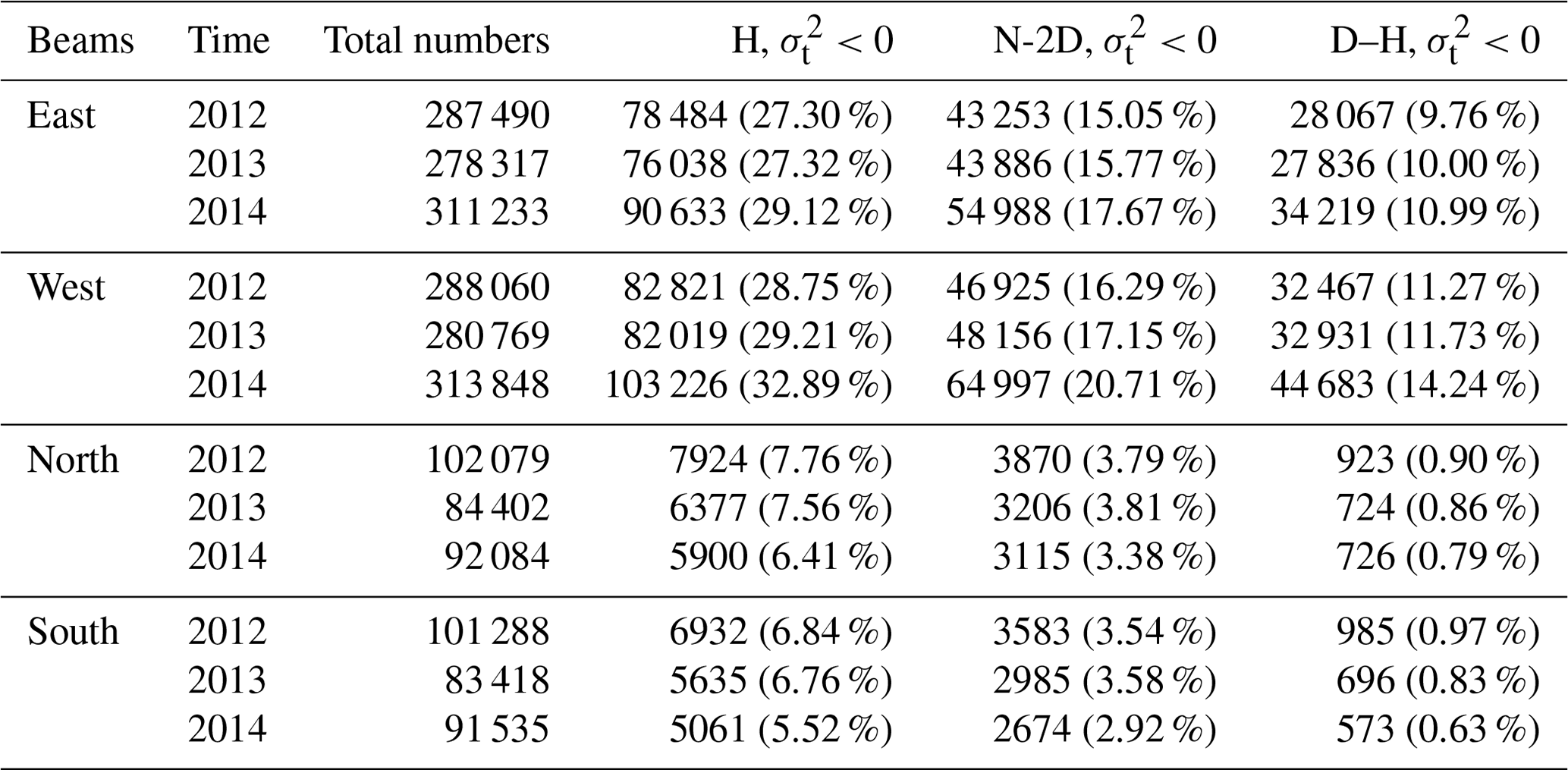
Using the observational data of four oblique beams within the range of 3–19.8 km from 2012 to 2014, we counted the total number of effective values of the observational spectrum width and the total number of ${\mathit{\sigma }}_{\mathrm{t}}^{\mathrm{2}}<\mathrm{0}$, as shown in Table 2. The turbulence spectrum width ${\mathit{\sigma }}_{\mathrm{t}}^{\mathrm{2}}$ is calculated by the three models. The results of the symmetric beams are similar. For the east and west beams, the rates of N-TKE (${\mathit{\sigma }}_{\mathrm{t}}^{\mathrm{2}}<\mathrm{0})$ of the H model, N-2D model and D–H model are in the range of 27 %–32 %, 15 %–21 % and 9 %–15 %, respectively. And for the north and south beams, the rates are in the range of 5 %–8 %, 2 %–4 % and 0.6 %–1.0 %. The probability that the turbulence spectrum width is less than 0 calculated by the H model is higher than that of the other two models.

Table 2 Total frequency of ${\mathit{\sigma }}_{\mathrm{t}}^{\mathrm{2}}<\mathrm{0}$ in the range of 3–19.8 km.

We further analysed the two-dimensional frequency distribution characteristics of horizontal wind speed (0 to 100 m s⁻¹) and the vertical shear of horizontal wind speed (−0.004 to 0.004 s⁻¹) in the range of 3–19.8 km above the radar station when the spectrum width value detected by the radar was valid, as shown in Fig. 1. The east–west component of horizontal wind speed over the radar site is distributed between 0 and 60 m s⁻¹, and the vertical shear of the horizontal wind speed ranges from −0.014 to 0.014 s⁻¹. The north–south component of horizontal wind speed over the radar site is distributed between 0 and 20 m s⁻¹, and the vertical shear of the horizontal wind speed ranges from −0.014 to 0.014 s⁻¹.

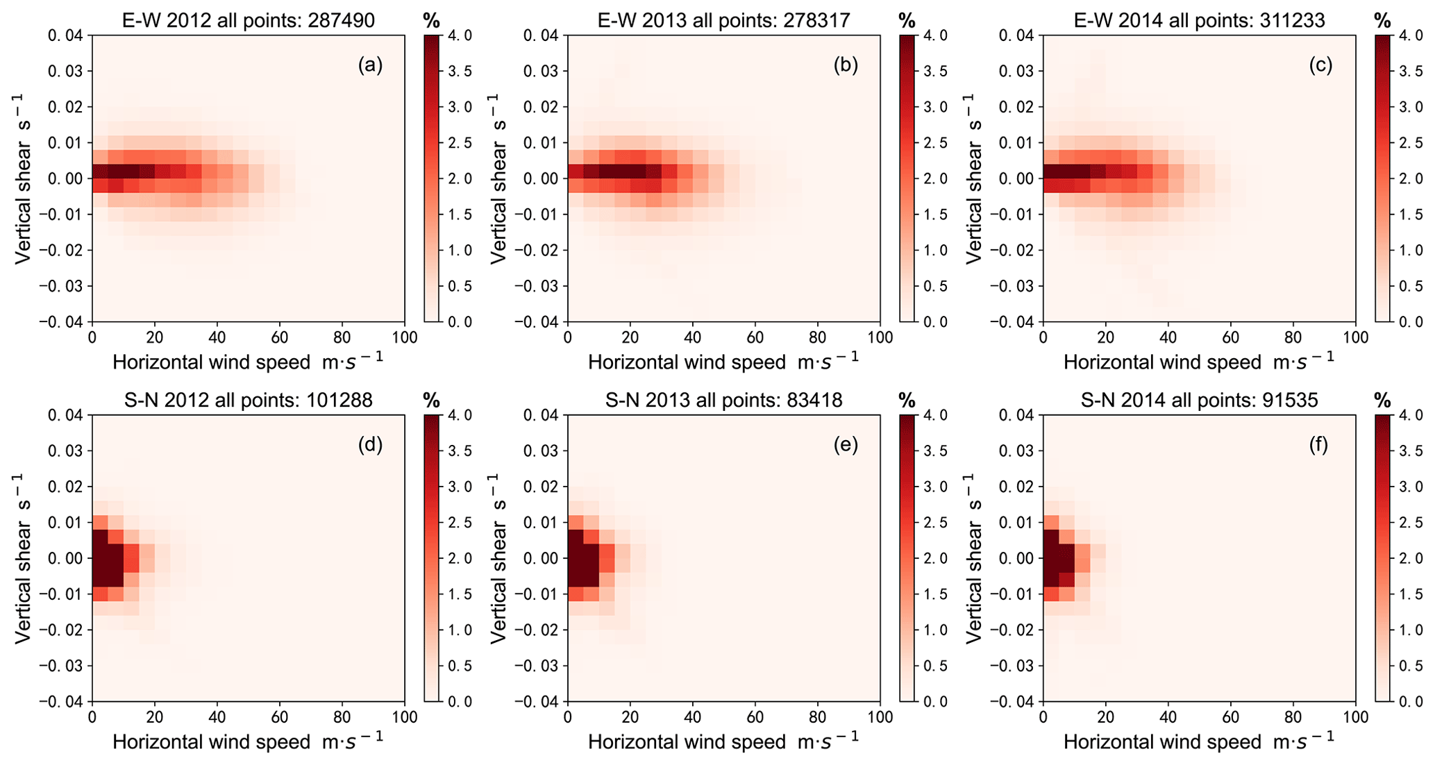
Figure 1 Two-dimensional frequency distribution characteristics of horizontal wind speed and vertical shear of horizontal wind speed within the height range of 3–19.8 km above the Beijing MST radar station from 2012 to 2014. (a, b, c) The east–west component of horizontal wind (d, e, f) the north–south component of horizontal wind.

3.1.1 Probability distribution characteristics of horizontal wind versus the vertical shear of horizontal wind observed by the Beijing MST radar

We further analysed the distributional characteristics of the horizontal wind speed (0 to 100 m s⁻¹) and vertical shear of horizontal wind speed (−0.004 to 0.004 s⁻¹) in the case of the N-TKE calculated by the three models. The north–south component of horizontal wind speed over the radar station is distributed between 0 and 20 m s⁻¹. This paper just gives the results of the east–west component of horizontal wind, as shown in Fig. 2a.1–a.3 and b.1–b.3. Meanwhile, Fig. 2c.1–c.3 shows the distributional characteristics of the three different models, $R^{-}\left(u,\frac{\partial u}{\partial z}\right)$, in the horizontal wind speed u and the vertical shear of horizontal wind $\frac{\partial u}{\partial z}$ domain. That is, the two-dimensional frequency distribution characteristics of u and $\frac{\mathrm{d}u}{\mathrm{d}z}$ in the Beijing area when ${\mathit{\sigma }}_{\mathrm{t}}^{\mathrm{2}}<\mathrm{0}$. $R^{-}=\frac{n_{ij}}{N^{-}}$, where n_ij is the frequency with negative ${\mathit{\sigma }}_{\mathrm{t}}^{\mathrm{2}}$ in a certain grid cell ($u_i\to u_{i+\mathrm{1}}$, ${\frac{\partial u}{\partial z}}_j\to {\frac{\partial u}{\partial z}}_{j+\mathrm{1}})$ and N⁻ is the total frequency of negative ${\mathit{\sigma }}_{\mathrm{t}}^{\mathrm{2}}$, as shown in Table 2. A total of 3 years of data from the Beijing MST radar from 2012 to 2014 are used.

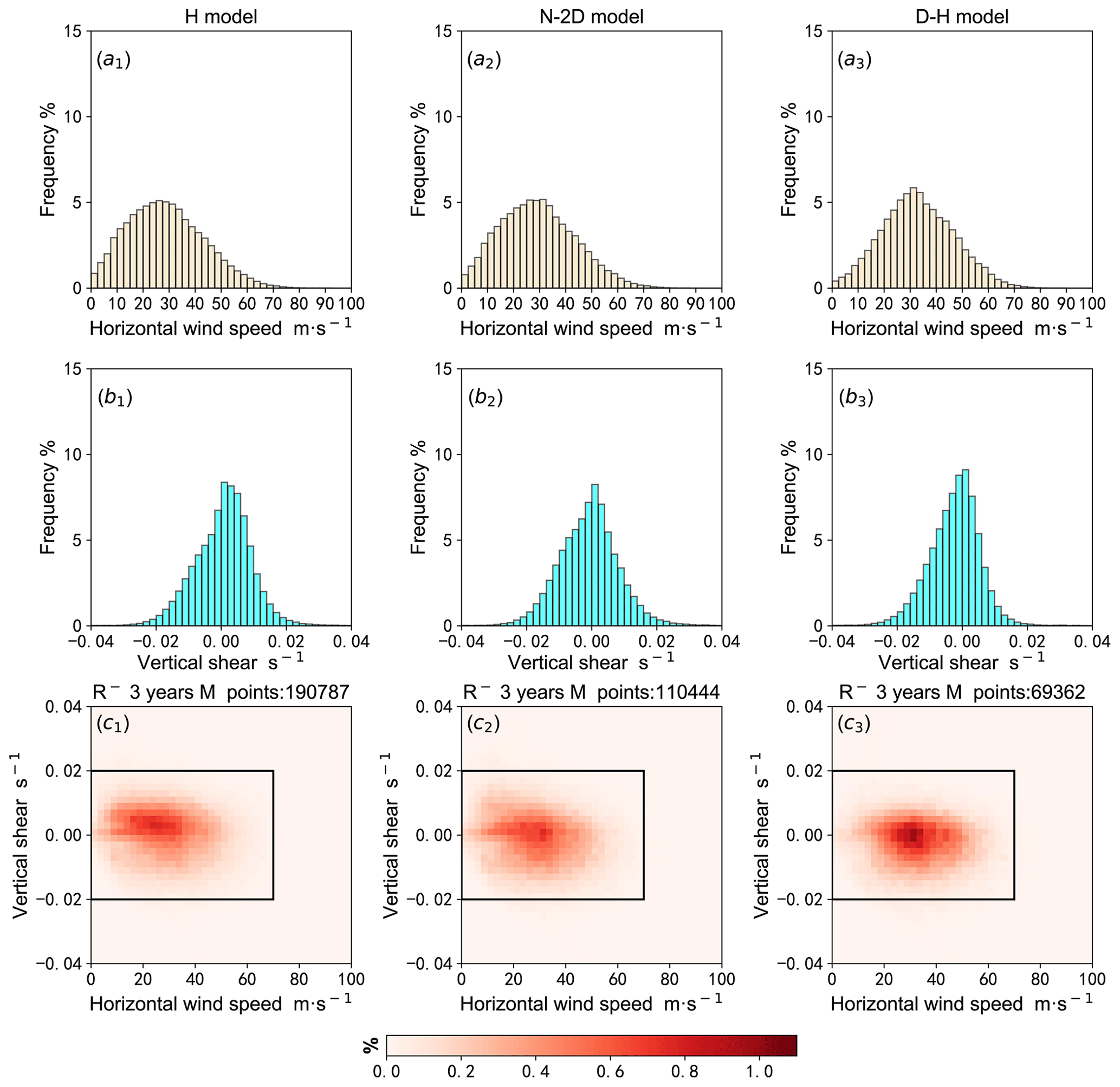
Figure 2 Frequency distribution of (a.1–a.3) horizontal wind speed and (b.1–b.3) the vertical shear of horizontal wind speed, along with (c.1–c.3) the two-dimensional frequency distribution characteristics of horizontal wind speed and the vertical shear of horizontal wind speed for the H model (a.1, b.1, c.1), N-2D model (a.2, b.2, c.2) and D–H model (a.3, b.3, c.3) when the turbulent kinetic energy is negative.

As shown in Fig. 2a.1, b.1, the medians of u and $\frac{\partial u}{\partial z}$ of the H model are about 27.5 m s⁻¹ and 0 s⁻¹, respectively. The u and $\frac{\partial u}{\partial z}$ are respectively distributed within 0 to 70 m s⁻¹ and −0.025 to 0.025 s⁻¹, where the frequency distribution of u has a heavy-tailed distribution that is obviously to the left, and the frequency distribution of $\frac{\partial u}{\partial z}$ appears as a rightward heavy-tailed distribution. For the N-2D model and D–H model, the frequency distribution characteristics of u and $\frac{\partial u}{\partial z}$ are relatively consistent with those of the H model. As shown in Fig. 2a.2, b.2, the medians of u and $\frac{\partial u}{\partial z}$ of the N-2D model are about 28.3 m s⁻¹ and 0 s⁻¹, respectively. The u and $\frac{\mathrm{d}u}{\mathrm{d}z}$ are respectively distributed within 0 to 70 m s⁻¹ and −0.025 to 0.03 s⁻¹. As shown in Fig. 2a.3, b.3, the medians of u and $\frac{\partial u}{\partial z}$ of the D–H model are about 32.4 m s⁻¹ and 0 s⁻¹, respectively. The u and $\frac{\mathrm{d}u}{\mathrm{d}z}$ are respectively distributed within 0 to 70 m s⁻¹ and −0.03 to 0.02 s⁻¹. The N⁻ value of the H model (total number of ${\mathit{\sigma }}_t^{\mathrm{2}}<\mathrm{0}$ values) is greater than that of the N-2D and D–H models, but the R⁻ values of the three models are mainly within the range of 0 to 80 m s⁻¹ and −0.02 to 0.02 s⁻¹, as shown in Fig. 2c.1–c.3. We also analysed the wind field distribution characteristics of different years (2012, 2013 and 2014) when ${\mathit{\sigma }}_{\mathrm{t}}^{\mathrm{2}}<\mathrm{0}$, and the results are similar to those in Fig. 2 (figures not shown).

3.1.2 Distributional characteristics of negative ${\mathit{\sigma }}_{\mathrm{tur}}^{\mathrm{2}}$ for the three methods

As shown in Fig. 2c.1–c.3, when the three models are used to calculate the turbulence spectrum width over the radar site, the values of R⁻ are significantly different in different ranges of u and $\frac{\partial u}{\partial z}$. That is, the probability of N-TKE has a different dependence on horizontal wind speed and the vertical shear of horizontal wind speed.

Due to the specific locality of the wind field distribution characteristics, the total samples of each grid cell ($u_i\to u_{i+\mathrm{1}}$, ${\frac{\partial u}{\partial z}}_j\to {\frac{\partial u}{\partial z}}_{j+\mathrm{1}})$ in Fig. 2c.1–c.3 are different. To analyse the universal relationship between the probability of N-TKE and both the horizontal wind speed and vertical shear in the three models, it is necessary to consider the difference in the number of total samples. Therefore, we further statistically analysed the probability of occurrence of N-TKE in each region of horizontal wind speed and vertical shear of horizontal wind speed ($R_{\mathrm{a}}^{-}$) calculated by the three models in each year of 2012–2014, as shown in Fig. 3. The definition of $R_{\mathrm{a}}^{-}$ is $R_{\mathrm{a}}^{-}=\frac{n_{ij}}{N_{{\mathrm{a}}_{ij}}}$, where n_ij is the frequency of ${\mathit{\sigma }}_{\mathrm{t}}^{\mathrm{2}}<$0 and $N_{{\mathrm{a}}_{ij}}$ is the total frequency for which ${\mathit{\sigma }}_{\mathrm{t}}^{\mathrm{2}}$ is a valid value in the grid cell ($u_i\to u_{i+\mathrm{1}}$, ${\frac{\partial u}{\partial z}}_j\to {\frac{\partial u}{\partial z}}_{j+\mathrm{1}}$).

Figure 3 Distribution of $R_{\mathrm{a}}^{-}$ for the (a.1) H model, (a.2) N-2D model and (a.3) D–H model in 2012. Panels (b.1)–(b.3) and (c.1)–(c.3) are the same as (a.1)–(a.3) but for the results of the three models in 2013 and 2014, respectively.

Based on mid-mode data of the Beijing MST radar, the distributional characteristics of the $R_{\mathrm{a}}^{-}$ calculated by the three methods are shown in Fig. 3. All samples are in the range of 0 to 80 m s⁻¹ and −0.02 to 0.02 s⁻¹, observed by four oblique beams. In fact, when the observations of four oblique beams were taken as the four groups of samples, the results were relatively consistent, although the horizontal wind component of the north and south beams was concentrated in 0 to 20 m s⁻¹. Therefore, this paper gives the result of taking four oblique beams as a total sample, as shown in Fig. 3. The results show that the effective data rate of each area is greater than 0.2 %. It can be seen that $\frac{\partial u}{\partial z}$ is between −0.012 and 0.012 s⁻¹, and u is between 0 and 60 m s⁻¹. Regardless of which model is used, the distributional characteristics of $R_{\mathrm{a}}^{-}$ with (u, $\frac{\partial u}{\partial z}$) in each year of 2012–2014 are consistent for the same model. The $R_{\mathrm{a}}^{-}$ of the H model can reach 70 %, and the probability of occurrence of N-TKE is significantly higher than that of the other two models. Furthermore, the $R_{\mathrm{a}}^{-}$ of the N-2D model and the D–H model ranges from 0 % to 45 % and 0 % to 35 %, respectively.

For the H model (Fig. 3a.1, b.1, c.1), $R_{\mathrm{a}}^{-}$ is sensitive to the magnitude of the horizontal wind speed (u) and the vertical shear of the horizontal wind speed (the absolute value, $\left|\frac{\partial u}{\partial z}\right|)$, but $R_{\mathrm{a}}^{-}$ is more sensitive to $\left|\frac{\partial u}{\partial z}\right|$. When the vertical shear of the horizontal wind speed is between −0.004 and 0.004 s⁻¹ and the horizontal wind speed is less than 30 m s⁻¹, the $R_{\mathrm{a}}^{-}$ has a relatively small value (<20 %). When the $\left|\frac{\partial u}{\partial z}\right|$ is greater than 0.006 s⁻¹, the N-TKE of the H model increases sharply with $\left|\frac{\partial u}{\partial z}\right|$, and the increasing rate $\frac{R_{\mathrm{a}}^{-}}{\left|\frac{\partial u}{\partial z}\right|}$ is about $\frac{\mathrm{20}\mathit{\%}}{\mathrm{0.002}{\mathrm{s}}^{-\mathrm{1}}}$. The result shows clearly that $R_{\mathrm{a}}^{-}$ increases with the horizontal wind speed and the absolute value of the vertical shear of the horizontal wind speed.

For the N-2D model (Fig. 3a.2, b.2, c.2), the result is similar to that of the H model when the vertical shear of the horizontal wind speed is less than 0 s⁻¹ ($\frac{\partial u}{\partial z}<\mathrm{0}$ s⁻¹). Of course, the $R_{\mathrm{a}}^{-}$ of the H model is greater. But when $\frac{\partial u}{\partial z}>\mathrm{0}$ s⁻¹, the $R_{\mathrm{a}}^{-}$ has a relatively higher value (>20 %) only if $\frac{\partial u}{\partial z}$ is greater than 0.008 s⁻¹. For the D–H model (Fig. 3a.3, b.3, c.3), the result is similar to N-2D model except that the vertical shear of the horizontal wind speed is greater than 0.006 s⁻¹. When $\frac{\partial u}{\partial z}>\mathrm{0.006}$ s⁻¹, the $R_{\mathrm{a}}^{-}$ of the N-2D model increases with $\frac{\partial u}{\partial z}$, and $R_{\mathrm{a}}^{-}$ is in the range of 10 % to 45 %, while the $R_{\mathrm{a}}^{-}$ of the D–H model is less than 10 %.

3.2 Distributional characteristics of negative ${\mathit{\sigma }}_{\mathrm{tur}}^{\mathrm{2}}$ as a function of height for the three models over the radar site

According to the above analysis, the three models for calculating the turbulence spectrum width have obvious differences in the dependence of the horizontal wind speed and the vertical shear of horizontal wind. The radar site is located in the mid-latitude westerly zone in the Northern Hemisphere, and the horizontal wind field at each height has obvious seasonal changes. Therefore, we further analysed the variational characteristics of the proportion of N-TKE with height in different seasons obtained by the three models, and we provide a reference for better selection of applicable models. Based on the 3 years of observational data from the east and west beams, the annual average proportion of N-TKE and the average profile in February (winter) and July (summer) were obtained, as shown in Fig. 4.

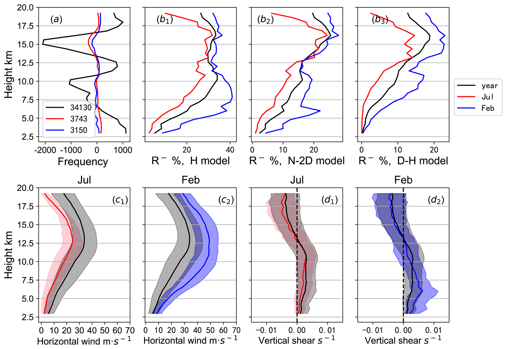
Figure 4 (a) Deviation profile of the data volume involved in the statistics and the mean value of the profile. The annual mean value is 34 130, the mean value in July is 3743 and the mean value in February is 3150. (b.1–b.3) Probability of N-TKE in each gate for the H model, N-2D model and D–H model, respectively. Panels (c.1), (c.2) and (d.1), (d.2) are the median, upper and lower quartile profiles of horizontal wind speed and the vertical shear of horizontal wind speed, respectively. Black, red and blue represent the characteristics of the year, July and February, respectively. A total of 3 years of radar observational data from 2012 to 2014 were used in the statistics.

As shown in Fig. 4a, within the range of 3–19.8 km, the average number of effective detections at all altitudes for the 3 years from 2012 to 2014 is 34 130. The average number of effective detections at all altitudes in July and February is 3743 and 3150, respectively.

The annual average profile of the proportion of N-TKE calculated by the three methods is shown in Fig. 4b.1–b.3 (solid black line). The proportion of N-TKE first increases and then decreases with altitude. All three models have peak values at 10–11 and 15–16 km. In these altitudinal ranges, there is strong vertical shear (positive at 10–11 km and negative at 15–16 km), and the horizontal wind speed is large in the range of 10–11 km (Fig. 4c.1, c.2, d.1, d.2). The maximum value of the ratio of N-TKE from the H model is about 35 % at 10 km, the maximum value of the N-2D model is about 25 % at 16 km and the maximum value of the D–H model is about 20 % at 16 km.

For the H model and N-2D model (Fig. 4b.1, b.2), compared with the annual distribution, the proportion of N-TKE in winter (February) increases at an altitude of 12 km below, and the proportion of N-TKE decreases in summer (July). This is mainly related to the fact that the vertical shear of the horizontal wind speed ($\frac{\partial u}{\partial z}$) at the altitude of 10 km below in winter (the upper quartile of $\frac{\partial u}{\partial z}$ is greater than 0.006 s⁻¹) is higher than that in summer (Fig. 4d.1, d.2), and the horizontal wind speed (u) in winter is higher than that in summer at all altitudes (Fig. 4c.1, c.2). In the range of 12–16 km, the vertical shear of horizontal wind speed has no obvious seasonal variation, and there is no significant difference between the annual profile and the monthly profile for the proportion of N-TKE.

For the D–H model, the annual mean and monthly mean (February and July) profiles of the rate of N-TKE are less than 10 % below 7.5 km, and the vertical shear of the horizontal wind speed ($\frac{\partial u}{\partial z}$) in this height range is positive. The result in Sect. 3.1 showed that when $\frac{\partial u}{\partial z}$ is positive and u is less than 30 m s⁻¹, the proportion of N-TKE is less than 10 %. The proportion of N-TKE in winter is higher than that in summer at all altitudes (Fig. 4b.3), which is related to the fact that the horizontal wind speed in winter is higher than that in summer at all altitudes.

3.3 Annual mean profile of turbulence parameters estimated using the three methods

The proportion of N-TKE can be a reference for the selection of the turbulence spectrum width calculation model to some extent. However, whether there are differences in the distributional characteristics of turbulence parameters calculated by the three models of the spectral width method requires further analysis. From 2012 to 2014 over the radar site, the distributions at each height of the observed spectral width, B–V frequency, turbulence dissipation rate obtained by the three calculation models, vertical turbulence diffusion coefficient, beam-shear broadening and distribution of spectral width caused by turbulence at each height are shown in Fig. 5. This study takes the observations of four oblique beams as a total sample.

The turbulence spectrum width contains negative values, as do ε and K_z. The difference between including negative values and excluding them is closely related to the proportion of N-TKE. Compared with the H model, the difference between including negative values and excluding them is very small for the N-2D model and D–H model, which is due to the fact that the H model has a higher proportion of N-TKE. The ratios of the median mean ε calculated by the H model, N-2D model and D–H model (including/excluding negative values) are $\mathrm{0.0010}/\mathrm{0.0019}$, $\mathrm{0.0017}/\mathrm{0.0017}$ and $\mathrm{0.0011}/\mathrm{0.0013}$, respectively. The ratio of K_z is $\mathrm{1.54}/\mathrm{2.55}$, $\mathrm{2.40}/\mathrm{2.40}$ and $\mathrm{1.53}/\mathrm{1.73}$, respectively. Several studies showed that the mean energy dissipation rates without negative values included will be quite large compared to that calculated from both positive and negative values (Kurosaki et al., 1996; Dehghan and Hocking, 2011). One of the exceptions is Kohma et al. (2019), who used an algorithm developed by Nishimura et al. (2020) to estimate the beam broadening component accurately. As a result, the difference of medians with and without negative energy dissipation rates is small.

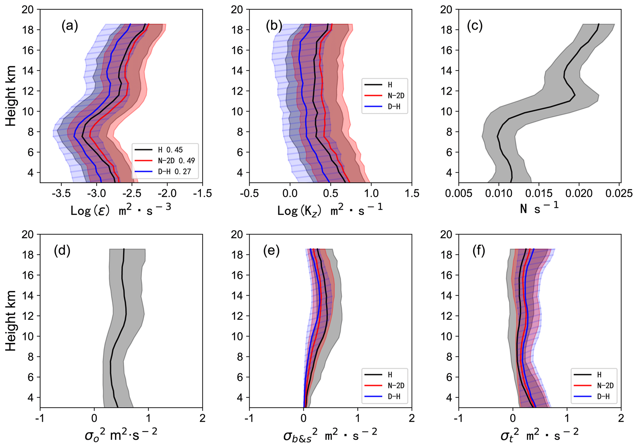
Figure 5 Profiles of (a) ε, (b) K_z, (c) B–V frequency, (d) observation spectrum width, (e) beam and shear broadening, and (f) spectrum width caused by turbulence. The solid line is the median, and the shaded area is the upper and lower quartiles. In panels (a), (b), (e) and (f), the black, red and blue solid lines and shaded areas represent the median and upper and lower quartiles of the H model, N-2D model and D–H model, respectively.

The distributional characteristics of the observed spectrum width calculated by Gaussian fitting are shown in Fig. 5d. The quartile of ${\mathit{\sigma }}_{\mathrm{o}}^{\mathrm{2}}$ (square of the Doppler velocity spectrum width) is between 0.2 and 1 m² s⁻². ${\mathit{\sigma }}_{\mathrm{o}}^{\mathrm{2}}$ increases with the altitude in the 7–13 km area, and ${\mathit{\sigma }}_{\mathrm{o}}^{\mathrm{2}}$ does not change much in the altitudinal range below 7 and above 13 km. The B–V frequency is distributed between 0.01 and 0.025 s⁻¹, as shown in Fig. 5c.

For the turbulent energy dissipation rate ε, the H model has c₁=0.45, the N-2D model has $c_{\mathrm{1}}=A^{-\frac{\mathrm{3}}{\mathrm{2}}}\approx \mathrm{0.49}$ and the D–H model has c₁=0.27 in this study. Figure 5a, b show the average profiles of the turbulence parameter years ε and K_z calculated by the H model, N-2D model and D–H model. The distribution of ${\mathit{\sigma }}_{\mathrm{t}}^{\mathrm{2}}$ according to the N-2D model and D–H model is very consistent. The trends with height of ${\mathit{\sigma }}_{\mathrm{t}}^{\mathrm{2}}$ are similar for the three models, when ${\mathit{\sigma }}_{\mathrm{t}}^{\mathrm{2}}$ calculated by the H model is smaller than that of the N-2D and D–H models at all heights (Fig. 5f). As shown in Fig. 5e, the beam and shear broadening ${\mathit{\sigma }}_{\mathrm{b}\mathrm{\&}\mathrm{s}}^{\mathrm{2}}$ calculated by the H model are distributed discretely and are larger than the calculation results of the other two models at each height.

Within the range of 3–19.8 km, there are differences in the ε calculated by the three models, but there is good consistency in the trend of changes in height, as shown in Fig. 5a. The ε decreases with altitude from 3 to 7 km, increases with altitude from 7 to 12 km, decreases slowly with altitude from 12 to 14 km and increases with altitude above 14 km.

Using the H model, N-2D model and D–H model, the distribution ranges of the ε (the upper and lower quartiles) are 10^−3.6–10^−2.1, 10^−3.4–10^−2.0 and 10^−3.6–10^−2.3 m² s⁻³, respectively. At an altitude of about 7 km, the ε calculated by the three models reaches a minimum in each case, where the medians of the H model, N-2D model and D–H model are 10^−3.2, 10^−3.1 and 10^−3.3 m² s⁻³, respectively. At 12 km, the medians of ε in the H model, N-2D model and D–H model are 10^−2.7, 10^−2.6 and 10^−2.8 m² s⁻³, respectively.

It can be seen from Eq. (2) that the value of c₁ and the calculated turbulence spectrum width of different models have an impact on the calculation result of ε. If the value of c₁ is constant, then only the values of ε are affected, not the characteristic of ε varying with height. The distributional characteristics of the turbulence spectrum width at each height calculated by the D–H model and N-2D model are similar, but the turbulence spectrum width calculated by the H model is smaller at all heights (Fig. 5f). The values of c₁ are 0.45 (H model), 0.49 (N-2D model) and 0.27 (D–H model) in this study. As a result, the values of ε calculated by the N-2D model are the largest at each height, when the values of the D–H model are the smallest. Therefore, the value of c₁ is an important issue that needs more research but is not the focus of this paper.

For the vertical turbulence dissipation coefficient K_z, within the range of 3–19.8 km, the values of K_z calculated by the three models are different, but there is a good consistency with the changing trend of the height: K_z first decreases and then increases as the height increases. The medians of the K_z calculated by the H model, N-2D model and D–H model are respectively within 10^0.3–10^0.7, 10^0.4–10^0.7 and 10^0.1–10^0.5 m² s⁻¹. The distributional ranges of the upper and lower quartiles are 10^0.0–10^0.9, 10^0.0–10¹ and 10^−0.2–10^0.7 m² s⁻¹, respectively.

4 Discussion

4.1 Applicability of the models in events

According to the probability of N-TKE in the three calculation models of the spectral width method, the applicability of the three models under different conditions can be judged. Under the state that the N-TKE accounts for a relatively large amount, the applicability of the corresponding model needs to be considered. For example, when the $\left|\frac{\partial u}{\partial z}\right|$ is greater than 0.006 s⁻¹, the N-TKE of the H model increases sharply with $\left|\frac{\partial u}{\partial z}\right|$, up to 60 %. In the area above 7.5 km over the radar site, the annual statistical results show that the N-TKE of the H model accounts for more than 20 %. Taking the east beam observations for example, as shown in Fig. 6b, in the area above 7.5 km over the radar site in July 2014, the probability of the N-TKE of the H model is relatively high, so the applicability of the H model is lacking in this area.

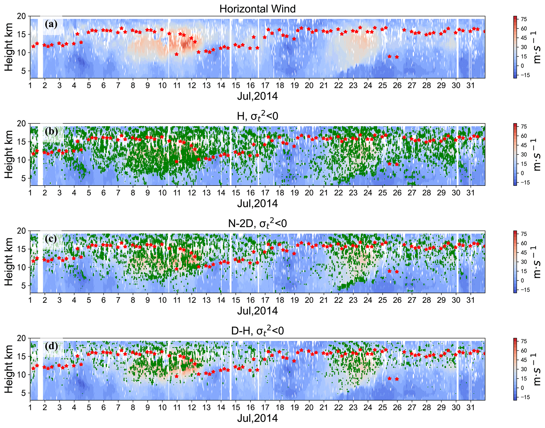
Figure 6 N-TKE distribution of three models over the Beijing MST radar site in July 2014: (a) the east–west component of horizontal wind; (b–d) area of N-TKE (green shading) for the east beam using the (b) H model, (c) N-2D model and (d) D–H model. The red scattered points are the tropopause.

Even when the statistical value of the probability of occurrence of the N-TKE of the model is low, the applicability of the model still needs to be considered in some atmospheric processes. For example, for the N-2D and D–H models, when the horizontal wind speed and the vertical shear of horizontal wind speed are within 0 to 60 m s⁻¹ and −0.02 to 0.02 s⁻¹, the rates of N-TKE are less than 45 % and 35 %, respectively. In fact, the values are higher in certain time period and height ranges, which is related to atmospheric processes and events indicated by the change of tropopause height. That is to say, we should pay more attention when dealing with the case studies. It also indicates the necessity to develop a universal model to calculate atmospheric turbulence parameters under the higher horizontal wind speed and vertical shear of horizontal wind speed circumstances. As shown in Fig. 6c, d, there were two tropopause folding processes in the Beijing area in July 2014, and the horizontal wind speed was greater than 60 m s⁻¹ in the range of 10–15 km during 8–13 and 23–24 July. In the strong-wind area, the proportions of N-TKE in the N-2D model and D–H model are higher. The results show that the N-2D model and D–H model, which have a relatively low rate of N-TKE, still need to be modified to consider the model's applicability during the process of strong wind speed or strong vertical shear.

4.2 Turbulence dissipation rate obtained using the middle and low modes

The characteristics of the changes in ε with height calculated by the mid-mode observational data of the Beijing MST radar agree well with existing research results. However, there is a difference in the range of values. The distributional characteristics of the median turbulence parameters of the Beijing MST radar are shown in Table 3.

Table 3 Turbulence parameters of the Beijing MST radar (39.78^∘ N, 116.95^∘ E) at the range of 3–19.8 km.

In addition to geographical differences, compared with other MST radars, the radial range resolution of the Beijing MST radar (600 m – other radars are generally 150 m) is the most different radar parameter. When using the spectral width method, it is necessary to satisfy the assumption that the observed atmospheric turbulence scale is smaller than the radar sampling volume. To verify the impact of range resolution, we used the low-mode data (radial resolution of 150 m) of the Beijing MST radar to calculate turbulence parameters, and then we compared them with the mid-mode results.

Based on the 3–7.8 km low-mode (mid-mode) data of the Beijing MST radar from 2012 to 2014, the H model, N-2D model and D–H model were applied, respectively. For east and west beams, the median ε is 10^−3.2 (10^−2.9) m² s⁻³, 10^−3.2 (10^−2.8) m² s⁻³ and 10^−3.4 (10^−3.1) m² s⁻³, respectively. For north and south beams, the median ε is 10^−3.0 (10^−2.7) m² s⁻³, 10^−2.9 (10^−2.7) m² s⁻³ and 10^−3.2 (10^−2.9) m² s⁻³, respectively. The H model has c₁=0.45, the N-2D model has $c_{\mathrm{1}}=A^{-\frac{\mathrm{3}}{\mathrm{2}}}\approx \mathrm{0.49}$, and the D–H model has c₁=0.27. Also, the ratio of the median ε of the middle and low modes is 10^0.3 (approximately 2.0). The distributional characteristics of ε obtained by applying the three models in the middle and low modes are basically the same, as shown in Fig. 7. The distribution of ε obtained by the H model is between 10⁻⁵ and 10^−1.5 m² s⁻³, which is more discrete than the results of the other two models: the ε obtained by the N-2D model and the D–H model is distributed between 10^−4.5 and 10^−1.5 m² s⁻³.

Figure 7 Distribution of ε in the middle and low modes of the Beijing MST radar in the range of 3–7.8 km from 2012–2014: (a.1–a.3) distributional characteristics of ε in the H model, N-2D model and D–H model (mid-mode); (b.1–b.3) as in (a.1–a.3) but for low-mode data. The grey bars are the result of north and south beams, and the yellow bars are based on the east and west beams.

The Beijing MST radar and the Harrow VHF (very high frequency) radar (42.04^∘ N) are at similar latitudes, and their ranges of tropospheric ε calculated by the H model show good consistency. The radial range resolution of the Harrow VHF radar is 500 m, and the ε is mainly distributed between 10⁻⁴ and 10⁻² m² s⁻³ in the altitudinal range of 1.5–11 km above the radar site. There is also a certain proportion in the range of 10⁻⁵–10⁻⁴ and 10⁻²–10^−1.5 m² s⁻³. The ε calculated using the ozone sounding (500–1000 m south of the Harrow radar) data is consistent with the radar calculation (Kantha and Hocking, 2011).

The above results show that the radial range resolution will affect the values of the turbulence parameters, but the effect is relatively small. There are other reasons for the difference in turbulence parameters calculated by different radar data. For example, when the dynamic stability is different, the value of ε may be different. The gradient Richardson number (Ri) is a dimensionless number used to judge dynamic stability. In Li et al. (2016), MAARSY radar (69.03^∘ N, 16.04^∘ E) data were used to calculate ε, revealing that when Ri was <1, the median ε was $\mathrm{5.18}\times {\mathrm{10}}^{-\mathrm{4}}$ m² s⁻³ (W kg⁻¹), and when Ri was >1, the median ε was $\mathrm{1.61}\times {\mathrm{10}}^{-\mathrm{4}}$ m² s⁻³ (the former being 3.2 times that of the latter).

5 Conclusion

Based on the quality-controlled spectral width data of the Beijing MST radar from 2012 to 2014, including more than 37 000 profiles for each oblique beam, three calculation models were used to calculate the turbulent spectral width. The turbulence parameters (ε, K_z) over the station were calculated by the turbulent spectral width. Furthermore, the relationship between the proportion of N-TKE and both the domain of the horizontal wind speed and the vertical shear of horizontal wind was analysed. The features of ε using the mid- and low-mode observation models were compared, and the conclusions can be summarised as follows.

1. The proportion of N-TKE in the H model, N-2D model and D–H model is sensitive to the horizontal wind. The ratio of N-TKE in the H model increases with the horizontal wind speed u and vertical shear of horizontal wind speed $\frac{\partial u}{\partial z}$, up to 60 %. The maximum values of the ratio in N-TKE in the N-2D model and D–H model are 45 % and 35 %, respectively. When the $\left|\frac{\partial u}{\partial z}\right|$ is greater than 0.006 s⁻¹, the N-TKE of the H model increases sharply with $\left|\frac{\partial u}{\partial z}\right|$; the increase rate is about $\frac{\mathrm{20}\mathit{\%}}{\mathrm{0.002}{\mathrm{s}}^{-\mathrm{1}}}$. For these three models, the results are similar except that the vertical shear of the horizontal wind speed is greater than 0.006 s⁻¹. When $\frac{\partial u}{\partial z}>\mathrm{0.006}$ s⁻¹, the proportion of N-TKE in the N-2D and H models increases with $\frac{\partial u}{\partial z}$, while the proportion in the D–H model is less than 10 % and has slight variation. Specially, the applicability of the N-2D model and D–H model should be considered in some weather processes with strong winds, such as the process of tropopause folding.

2. At all heights over the radar site, the horizontal wind speed in winter is greater than in summer. Therefore, the proportion of N-TKE at each height of the D–H model in winter is greater than that in summer. In the range of 12–16 km the vertical shear of horizontal wind speed has no obvious seasonal variation, and the H and N-2D models have no noticeable seasonal changes

3. Based on the observations of the Beijing MST radar in the altitudinal range of 3–19.8 km from 2012 to 2014, the median values of ε in the H model, N-2D model and D–H model are 10^−3.2–10^−2.7, 10^−3.0–10^−2.6 and 10^−3.3–10^−2.8 m² s⁻³, respectively. The median values of K_z in the three models are 10^0.3–10^0.7, 10^0.4–10^0.7 and 10^0.1–10^0.5 m² s⁻¹, respectively.

4. Compared with previous studies, the turbulence parameters obtained by the three models over the radar site have the same variational trend with height. Still, there are differences in the distributional ranges of the turbulence parameters. Further analysis shows that different radial range resolutions of the radar have no apparent effect on the distributional ranges of the turbulence parameters.

When the spectral width method is used to calculate radar-based turbulence parameters, the statistical results in this paper can provide a reference for the selection of the turbulence spectral width models. For example, when analysing the statistical characteristics of the turbulence parameters over the radar station, a more suitable calculation model can be selected based on the local wind factors. The current results show that a more general model to calculate radar-based turbulence parameters should be proposed in researching the changes of turbulence parameters in specific weather processes.