the Creative Commons Attribution 4.0 License.
the Creative Commons Attribution 4.0 License.
 | 29 Aug 2022
Combining Mie–Raman and fluorescence observations: a step forward in aerosol classification with lidar technology
Igor Veselovskii
Qiaoyun Hu
Philippe Goloub
Thierry Podvin
Boris Barchunov
Mikhail Korenskii
The paper presents an approach to revealing the variability in aerosol type, at high spatiotemporal resolution, by combining fluorescence and Mie–Raman lidar observations. The multiwavelength Mie–Raman lidar system in operation at the ATOLL (ATmospheric Observation at liLLe) platform, Laboratoire d'Optique Atmosphérique, University of Lille, has included, since 2019, a wideband fluorescence channel allowing the derivation of the fluorescence backscattering coefficient βF. The fluorescence capacity GF, which is the ratio of βF to the aerosol backscattering coefficient, is an intensive particle property, strongly changing with aerosol type, thus providing a relevant basis for aerosol classification. In this first stage of research, only two intensive properties are used for classification, namely the particle depolarization ratio at 532 nm, δ532, and the fluorescence capacity, GF. These properties are considered because they can be derived at high spatiotemporal resolution and are quite specific to each aerosol type. In particular, in this study, we use a δ532–GF diagram to identify smoke, dust, pollen, and urban aerosol particles. We applied our new classification approach to lidar data obtained during the 2020–2021 period, which includes strong smoke, dust, and pollen episodes. The particle classification was performed with a height resolution of about 60 m and temporal resolution better than 8 min.
- Article
(7977 KB) - Full-text XML
- BibTeX
- EndNote


Atmospheric aerosol is one of the key factors influencing the Earth's radiation budget through the absorption and scattering of solar radiation and by affecting cloud formation. The processes of aerosol–radiation and aerosol–cloud interaction depend on aerosol size, shape, morphology, absorption, solubility, etc.; thus, knowledge of the chemical composition and mixing state of the aerosol particles is important for modeling the aerosol impact (Boucher et al., 2013). The aerosol properties may vary in a wide range, so, in practice, usually several main types of aerosols are separated based on their origin, e.g., urban, dust, marine, and biomass burning (Dubovik et al., 2002). Successful remote characterization of the column-integrated aerosol composition from the observations of sun–sky photometers and spaceborne multiangle polarimeters has been demonstrated in numerous publications (Dubovik et al., 2002; Giles et al., 2012; Hamill et al., 2016; Schuster et al., 2016; Li et al., 2019; Zhang et al., 2020). The aerosol impacts, however, depend also on vertical variations/distributions of particle concentration and composition, which cannot be derived from these instruments.
One of the recognized remote sensing techniques for the vertical profiling of aerosol properties is lidar. Multiwavelength Mie–Raman lidar and HSRL (high spectral resolution lidar) systems provide a unique opportunity to derive height-resolved particle intensive properties, such as lidar ratios, Ångström exponents, and depolarization ratios at multiple wavelengths. Based on this information, the particle type can be determined (Burton et al., 2012, 2013; Groß et al., 2013; Mamouri and Ansmann, 2017; Papagiannopoulos et al., 2018; Nicolae et al., 2018; Hara et al., 2018; Voudouri et al., 2019; Wang et al., 2021; Mylonaki et al., 2021 and references therein). However, there is a fundamental difference between the particle classification based on the sun–sky photometer and on lidar observations. From direct Sun and azimuth scanning measurements of the photometer, more than 100 observations are available. From this information, the spectrally dependent refractive index and absorption Ångström exponent can be determined, which is important for aerosol classification (Schuster et al., 2016; Li et al., 2019). The commonly used multiwavelength lidars are based on a tripled Nd:YAG laser and are capable of providing three types of backscattering (355, 532, 1064 nm), two extinction (355, 532 nm) coefficients, and up to three particle depolarization ratios (so-called set). Thus, the number of available lidar observations is eight or less, which limits the performance of the aerosol classification algorithms. Nevertheless, the results obtained by different research groups demonstrate that lidar-based particle identification is possible. In the publications of Burton et al. (2012, 2013), a classification was performed based on four intensive parameters measured by the HSRL system, i.e., the lidar ratio at 532 nm (S532), the backscattering Ångström exponent for 532 and 1064 nm wavelengths (BAE), and particle depolarization ratios at 532 and 1064 nm (δ532 and δ1064). With these input parameters, there are eight aerosol types, i.e., smoke, fresh smoke, urban, polluted maritime, maritime, dusty mix, pure dust, and ice, discriminated.
Important information on aerosol vertical distribution comes from the EARLINET (European Aerosol Research Lidar Network) and ACTRIS (Aerosol, Clouds and Trace Gases Research Infrastructure) lidar network, aiming at unifying multiwavelength Mie–Raman lidar systems over Europe (Pappalardo et al., 2014). For the automation of aerosol classification, several approaches were developed in the frame of EARLINET. These approaches include the Mahalanobis distance-based classification algorithm (Papagiannopoulos et al., 2018), a neural network aerosol classification algorithm (NATALI; Nicolae et al., 2018), and an algorithm based on source classification analysis (SCAN; Mylonaki et al., 2021). All of these algorithms have demonstrated their ability for aerosol classification. In particular, NATALI is able to identify up to 14 aerosol mixtures from observations.
Nevertheless, the abovementioned algorithms have to deal with a fundamental limitation, namely that the particle intensive properties, even for pure aerosols (generated by a single source), exhibit strong variations. For example, the lidar ratio S355 of smoke in the publication of Nicolae et al. (2018) varies in the 38–70 sr range, and in our own measurements, we observed values for aged smoke S355 as low as 25 sr (Hu et al., 2022). Strong variation in the smoke lidar ratios in EARLINET/ACTRIS observations is discussed also in the recent publication of Adam et al. (2021). Such uncertainty in the parameters of the aerosol model complicates the aerosol classification. Thus, it is desirable to combine the Mie–Raman observations with another range-resolved technique that provides additional independent information about aerosol composition. Such information can be obtained from laser-induced fluorescence emissions.
The application of fluorescence lidar technique was intensively considered during the last decade to study aerosol particles. Lidar measurements of the full fluorescence spectrum with multi-anode photomultipliers (Sugimoto et al., 2012; Reichardt, 2014; Reichardt et al., 2018; Saito et al., 2022) provide an obvious advantage in particle identification. However, even a more simple fluorescence lidar with a single wideband fluorescence channel opens new opportunities for aerosol characterization (Veselovskii et al., 2021, 2022; Zhang et al., 2021). Such a fluorescence configuration could be implemented in existing Mie–Raman lidars, and the fluorescence backscattering coefficient βF is calculated from the ratio of fluorescence and nitrogen Raman signals. To characterize the aerosol fluorescence properties, the fluorescence capacity GF is introduced as the ratio of βF to aerosol backscattering coefficient at one of laser wavelengths (Veselovskii et al., 2020b). In this study, the backscattering at 532 nm was used. The fluorescence capacity is an intensive particle parameter, which changes strongly with aerosol type, with the highest value for smoke and the lowest for dust. Thus, the combination of Mie–Raman and fluorescence backscatter provides a basis to improve particle classification. A Mie–Raman lidar provides several particle-intensive parameters; however, the profiles of particle parameters associated with the extinction coefficient, such as the lidar ratio or extinction Ångström exponent, may contain strong noise because the extinction coefficients are derived from the slope of Raman lidar signals. Thus, averaging over the significant spatiotemporal intervals is demanded. Meanwhile, the particle depolarization and the fluorescence capacity can be calculated with a high spatiotemporal resolution.
Recently, we have demonstrated that the δ–GF diagram allows us to separate several aerosol types, such as dust, pollen, urban (continental), and smoke (Veselovskii et al., 2021). In the present study, we use this technique to classify aerosol particle types in the troposphere at a high spatiotemporal resolution. We present the results of aerosol classification on the basis of fluorescence and Mie–Raman lidar measurements performed at the ATOLL (ATmospheric Observation at liLLe) at Laboratoire d'Optique Atmosphérique, University of Lille, during 2020–2021, which includes strong smoke, dust, and pollen episodes. The paper starts with a description of the experimental setup and data processing scheme in Sect. 2. In Sect. 3, we present the algorithm for aerosol classification based on depolarization and fluorescence measurements. Results of the application of the developed approach to different atmospheric situations, including smoke, dust, and pollen episodes, are given in Sect. 4.
2.1 Lidar system
The multiwavelength Mie–Raman lidar LILAS (LIlle Lidar AtmosphereS) is based on a tripled Nd:YAG laser with a 20 Hz repetition rate and pulse energy of 70 mJ at 355 nm. Backscattered light is collected by a 40 cm aperture Newtonian telescope, and the lidar signals are digitized with Licel transient recorders with a 7.5 m range resolution, allowing simultaneous detection in the analog and photon counting mode. The system is designed for the detection of elastic and Raman backscattering, allowing the so-called data configuration, including three particle backscattering values (β355, β532, β1064) and two extinction (α355, α532) coefficients, along with three particle depolarization ratios (δ355, δ532, δ1064). The particle depolarization ratio, determined as a ratio of cross- and co-polarized components of the particle backscattering coefficient, was calculated and calibrated in the same way as described in Freudenthaler et al. (2009). Many calibration and operation procedures have been automated for the LILAS system to improve the overall performance of the lidar in terms of observation frequency and data quality. The aerosol extinction and backscattering coefficients at 355 and 532 nm were calculated from Mie–Raman observations (Ansmann et al., 1992), while β1064 was derived by using the Klett (1985) method. The full geometrical overlap was achieved at approximately 750 m range. For the calculation of α and β at 532 nm, we use the rotational Raman scattering instead of the vibrational one (Veselovskii et al., 2015), which allows us to increase the power of Raman backscatter and to decrease separation between the wavelengths of elastic and Raman components. Additional information about atmospheric parameters was available from radiosonde measurements performed at Herstmonceux (UK) and Beauvechain (Belgium) stations, located 160 and 80 km away from the observation site, respectively.
The LILAS system can also profile the laser-induced fluorescence of aerosol particles. A part of the fluorescence spectrum is selected by a wideband interference filter of 44 nm width centered at 466 nm. The strong sunlight background during the daytime restricts the fluorescence observations to nighttime hours. The fluorescence backscattering coefficient, βF, is calculated from the ratio of fluorescence and nitrogen Raman backscattering signal, as described in Veselovskii et al. (2020b). This approach allows us to evaluate the absolute values of βF, if the relative sensitivity of the channels is calibrated and the nitrogen Raman scattering differential cross section is known. All βF profiles presented in this work were smoothed with the Savitzky–Golay method, using second-order polynomials with 21 points in the window. For the calculation of the fluorescence capacity GF, in principle, backscattering coefficients at any laser wavelength can be used. In our study, we always used β532 because it is calculated with the use of a rotational Raman component and is considered to be the most reliable; thus, the fluorescence capacity is calculated as .
2.2 Calculation of the particle backscattering coefficient from Mie–Raman measurements
Mie–Raman lidar measurements allow the independent evaluation of aerosol extinction and backscattering coefficients. A commonly used approach for β calculation was formulated in the paper of Ansmann et al. (1992). This approach includes the choice of a reference height, where the scattering is purely molecular. However, such a height range is not always available, for example, in the presence of the low-level clouds. Moreover, when long-term spatiotemporal variations in backscattering coefficients are analyzed, then the uncertainty in the choice of the reference height leads to oscillations in β profiles. To resolve this issue, we modified the Raman method as described below.
In an elastic channel, the backscattered radiative power PL, at wavelength λ0 and distance z, is described by the lidar equation as follows:
while in a Raman channel, it can be written as follows:
Here O(z) is the geometrical overlap factor, which is assumed to be the same for elastic and Raman channels. CL and CR are the range independent constants, including the efficiency of the detection channel. TL and TR are one-way transmissions which describe light losses on the way from the lidar to distance z at laser λL and Raman λR wavelengths. Backscattering and extinction coefficients contain the following aerosol and molecular contributions: and , where the superscripts a and m indicate aerosol and molecular scattering, respectively. The Raman backscattering coefficient is as follows:
where N is the number of Raman scatters (per unit of volume), and σR is the Raman differential scattering cross section in the backward direction.
Dividing Eq. (1) into Eq. (2), we obtain the following:
The backscattering coefficient is calculated from Eqs. (3) and (4) as follows:
The differential transmission can be calculated in the same way as it is done for the water vapor measurements (Whiteman, 2003). For a rotational Raman signal, which we use in our 532 nm channel (Veselovskii et al., 2015), λL≈λR, so that = 1.
The calibration constant can be found by comparing in Eq. (5) with the backscattering coefficient computed with the traditional Raman method and using the reference height (Ansmann et al., 1992).
For simplicity, hereinafter we will use the notation βL instead of . Thus, if during the measurement session we have a temporal interval where the reference height is available, then we can determine the calibration constant K and use it for βL calculations from Eq. (5), assuming that the relative sensitivity of the channels during the session is not changed. Even if cloud layers occur during the whole session, we can use K from the previous cloud-free profiles (assuming, again, that the relative sensitivity of the channels is the same). We will call this approach for β calculation the modified Raman method to distinguish it from the traditional one (Ansmann et al., 1992).
To estimate variations in the relative sensitivity of the channels, we analyzed long-term cloudless measurements when the reference height was available for every individual profile. The results demonstrate that variations in the calibration constant during the session (about 8 h) were below 3 %. Figures 1 and 2 present the application of this modified Raman method to the measurements on 2 March 2021. The dust layer extended from 2 to 8 km height, and inside this layer, the ice and liquid clouds were formed during the 00:00–05:00 UTC interval; thus, β532 could not be calculated with the traditional Raman technique. The temporal interval of 19:00–20:00 UTC was used to find calibration constant K. Figure 1 shows the vertical profiles of backscattering coefficient , calculated with the traditional Raman method (with reference height), and β532 ,calculated with the modified method (with the calibration constant). Profiles of and β532 coincide for the whole height range. The calibration constant K, shown on the same plot, does not demonstrate height dependence, though oscillations around the mean value increase with height. For computations, we choose the value of K at low altitudes averaged inside some height interval.

Figure 1Backscattering coefficients at 532 nm for the period 19:00–20:00 UTC on 2 March 2021, calculated from Mie–Raman observations, using the same reference height as Ansmann et al. (1992; green) or the calibration constant as in Eq (5) (magenta). The profile of the calibration constant K is shown with a red line.
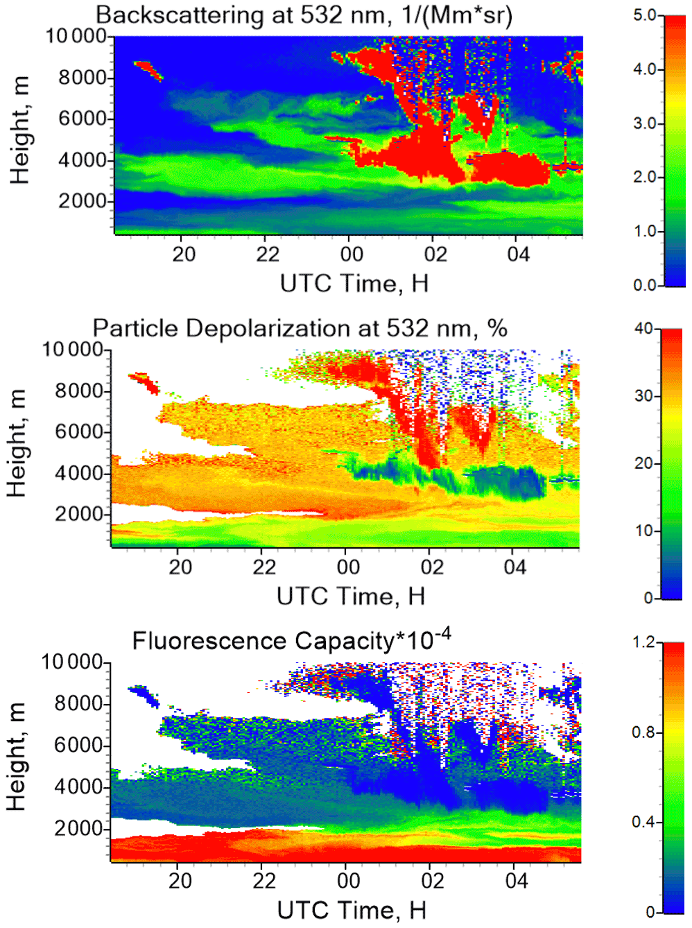
Figure 2Spatiotemporal distributions of the backscattering coefficient β532, the particle depolarization ratio δ532, and the fluorescence capacity GF on the night of 2–3 March 2021. The backscattering coefficient β532 is calculated with the modified Raman method. The values of δ532 and GF are shown for β532 > 0.2 Mm−1 sr−1.
Figure 2 provides spatiotemporal variations in β532, particle depolarization δ532, and the fluorescence capacity GF. Depolarization measurements reveal the presence of dust (δ532≈30 %) and the ice cloud above 4 km (δ532 > 40 %). The liquid cloud below 4 km after midnight can be identified by a low depolarization ratio δ532 < 3 %. The fluorescence capacity of dust is low, at about 0.2 × 10⁻⁴. However, below 2 km, GF is significantly higher, up to 1.2 × 10⁻⁴. In combination with a high depolarization ratio (up to 20 %), it can indicate the presence of pollen at low altitudes. On the fluorescence capacity panel, we can see that, after 01:00 UTC, the dust and pollen layers are mixed below 2 km, resulting in a value of GF of about 0.5 × 10⁻⁴. The fluorescence capacity inside ice and liquid clouds is below 0.01 × 10⁻⁴. Figure 2 clearly demonstrates the advantage of simultaneous depolarization and fluorescence measurements for the study of cloud formation in the presence of aerosol. All spatiotemporal distributions of β532 presented in this paper were calculated from Eq. (5) with a modified Raman method.
3.1 Approach for aerosol classification
As was discussed in our recent publication (Veselovskii et al., 2021), the δ-GF diagram allows us to separate several aerosol types, including smoke, dust, pollen, urban, and ice and liquid water particles. Smoke and urban aerosols both have a small depolarization ratio, but the fluorescence capacity of smoke is almost 1 order of magnitude higher, so these particles can be separated. Dust and pollen both have a high depolarization ratio (up to 30 %), but GF of dust is significantly lower, which again provides the basis for discrimination. The depolarization ratio of some aerosol types is characterized by a strong spectral dependence. For example, the depolarization ratio of aged smoke decreases with wavelength. It is below 5 % at 1064 nm, but at 355 nm in upper troposphere, it may exceed 20 % (Burton et al., 2015; Haarig et al., 2018; Hu et al., 2019; Veselovskii et al., 2022), which complicates the smoke and dust separation. For pollen, on the contrary, the depolarization ratio at 1064 nm can be the highest (Veselovskii et al., 2021). Thus, the choice of δ1064 for the δ-GF diagram could be advantageous. However, as already mentioned, the backscattering coefficient at 1064 nm is calculated with the Klett (1985) method, which, besides the assumptions about lidar ratio, needs a reference height and cannot be used in cloudy situations. This is why, in our study, we used the δ532-GF diagram.
In our present work, we consider a simple classification scheme since we use only two intensive parameters, GF and δ532. Our goal is to demonstrate that, in the δ532-GF diagram, our lidar observations form clusters and characteristic patterns which can be attributed to different aerosol types or their mixtures. We consider four aerosol types, i.e., dust, smoke, pollen and urban, and two cloud types, i.e., liquid and ice clouds. Dust and pollen are large particles of a complicated shape, characterized by high depolarization ratio, while smoke and urban pollution are small particles with low depolarization. In our classification, urban aerosol includes continental aerosol, sulfates, and soot. At this stage, we do not yet consider absorption to discriminate the particles.
The choice of the range of particle properties variations for each aerosol type is an important aspect of the approach. Typical ranges of GF and δ532 variations used in our classification scheme are given in Table 1 and are shown in Fig. 3. These ranges are based on results obtained in LOA (Laboratoire d'Optique Atmosphérique) and on results presented in aerosol classification studies (Burton et al., 2012, 2013; Nicolae et al., 2018; Papagiannopoulos et al., 2018; Mylonaki et al., 2021).
-
Dust. The depolarization ratio, δ532, of Saharan dust near the source regions is up to 35 % (Veselovskii et al., 2020a). However, after transportation and mixing with local aerosol, δ532 can be as low as 20 % (Rittmeister et al., 2017). In many studies, the dust events having a smaller depolarization ratio are classified as polluted dust (e.g., Burton et al., 2012, 2013). At the moment, we do not introduce the discrimination between the two subtypes and mark as dust the particles with 20 % < δ532 < 35 % and 0.1 × 10⁻⁴ < GF < 0.5 × 10⁻⁴.
-
Smoke. In 2021–2022, we regularly observed, over the ATOLL platform, smoke layers originating from Californian and Canadian forest fires (Hu et al., 2022). The particle depolarization and fluorescence capacity of this transported smoke varied from episode to episode, and for classification, we selected the ranges 2 % < δ532 < 10 % and 2 × 10⁻⁴ < GF < 6 × 10⁻⁴. At this stage, we do not discriminate between fresh and aged smoke, and the range of the δ532 variation is similar to the one used in the classification of Burton et al. (2012).
-
Pollen. The pollen over northern France is usually mixed with other aerosol, and the particles which we mark as pollen are actually the mixtures. The depolarization ratio of clean pollen varies strongly for different taxa. For birch pollen, Cao et al. (2010) reported δ532 = 33 %, and in the measurements over Finland during birch pollination, Bohlmann et al. (2019) observed values of δ532 up to 26 %. The observations over Lille during the pollen season (Veselovskii et al., 2021) rarely revealed values δ532 exceeding 20 %. Based on those observations, we classify as pollen the particles mixtures with 15 % < δ532 < 30 % and 0.8 × 10⁻⁴ < GF < 3.0 × 10⁻⁴.
-
Urban. This type of aerosol includes a variety of particle types (e.g., sulfates and soot), and its properties may depend on the relative humidity. Based on our measurements inside the boundary layer, for classification, we choose the ranges 1 % < δ532 < 10 % and 0.1 × 10⁻⁴ < GF < 1.0 × 10⁻⁴. A similar range for δ532 is used in the classification of Burton et al. (2013). Urban and smoke particles both have a low depolarization, but the smoke fluorescence capacity can be up to 1 order of magnitude higher, so these particles can be reliably discriminated.
-
Ice and water clouds. Both cloud types have low fluorescence capacity GF < 0.01 × 10⁻⁴. However, the ice clouds are usually observed at the heights where the fluorescence signal is low and cannot be used for classification. Thus, above ∼ 8 km, the ice cloud are identified by a high depolarization ratio δ532 > 40 %. The depolarization ratio of the liquid water clouds is usually affected by the effects of the multiple scattering, so for their identification, we use δ532 < 5 %.
Table 1Ranges of particle depolarization δ532 and fluorescence capacity GF, which were used for aerosol classification.
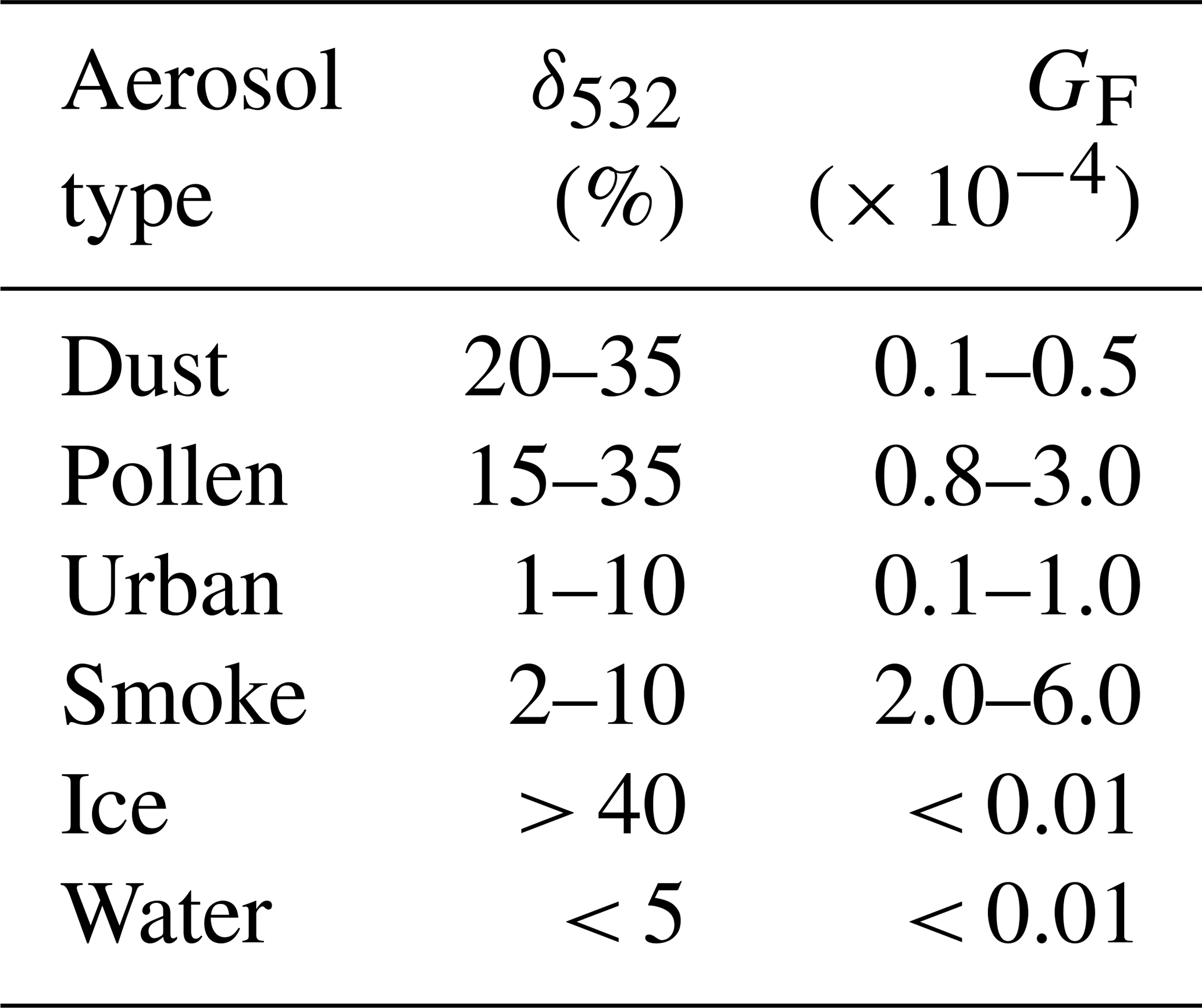
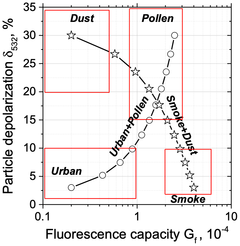
Figure 3Aerosol type with a δ532-GF diagram. The ranges of the particle parameter variations for dust, pollen, smoke, and urban aerosol are given by rectangles. The symbols show the results of simulation performed for pollen and urban (circles) and smoke and dust (stars) mixtures. The relative contribution of pollen (smoke) to the total backscattering β532 varied in the 0–1.0 range, with steps of 0.1. The particle parameters used in the calculations are given in the text.
The analysis of aerosol mixtures is an important subject, and the possibility to separate the mixture components based on lidar measurements was discussed in publications of Sugimoto and Lee (2006), Groß et al. (2011), Gasteiger and Freudenthaler (2014), Tesche et al. (2009), and Burton et al. (2014). The information about the mixture composition can be also revealed in the δ532–GF diagram. For example, pollen can be mixed with urban particles. At different heights, the pollen contributes differently to β532, so in the δ532–GF diagram, the data points will form the pattern, which extends from the location attributed to pure urban aerosol to the location attributed to pure pollen. To estimate how such a pattern looks, simplified modeling for fixed particle parameters was performed. The corresponding results are shown in Fig. 3 by the symbols (circles). The particle depolarization ratio δ of the mixture, containing urban aerosol (u) and pollen (p), with the depolarization ratios δu and δp, can be calculated as follows:
The fluorescence capacity of the mixture is given by the following:
Here, the total backscattering .
The computations in Fig. 3 were performed for values of the pollen contribution in the 0–1.0 range, with steps of 0.1. We assume that the depolarization ratios of pollen and urban aerosol are = 30 % and = 3 %, while the fluorescence capacities are = 0.2 × 10⁻⁴ and = 2.5 × 10⁻⁴. We remind the reader that the fluorescence capacities are calculated at 532 nm wavelength. In the δ532–GF diagram, the computed points provide a characteristic curve, which in the next section will be compared with experimental results. The same computations were performed for a smoke (s) and dust (d) mixture, assuming = 30 %, = 3 %, = 0.2 × 10⁻⁴, and = 4.0 × 10. The corresponding results are shown in Fig. 3 with stars. In a similar way, the characteristic curves for other mixtures can also be represented.
We are also able to identify liquid water and ice layers. Liquid water cloud layers have low fluorescence capacity (GF < 0.01 × 10⁻⁴) and δ532 < 3 %. Ice particles also have low GF, but at heights where ice clouds are usually observed, the signal of the fluorescence backscattering is noisy. Thus, at high altitudes, ice particles are discriminated by a high depolarization ratio δ532 > 40 %.
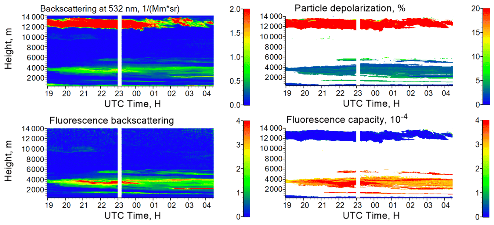
Figure 4Spatiotemporal distributions of the backscattering coefficient β532, the fluorescence backscattering coefficient βF (in 10−4 Mm−1 sr−1), the particle depolarization ratio δ532, and the fluorescence capacity GF on the night of 12–13 September 2020. The calculation of δ532 and GF was not performed for β532 < 0.2 Mm−1 sr−1. The values of the backscattering coefficient and the depolarization ratio of ice clouds are high (above 20 Mm−1 sr−1 and 40 %, respectively) and are off the scale for the maps presented.
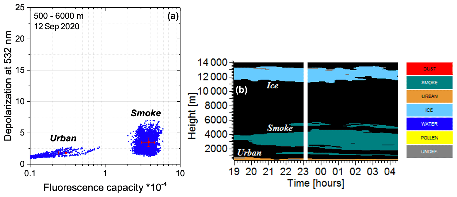
Figure 5(a) The δ532-GF diagram for the data from Fig. 4 in the 500–6000 m height range. Red crosses show the uncertainty of the measurements. (b) Spatiotemporal distribution of aerosol types on the night of 12–13 September 2020. The gray coloring shows undefined aerosol types, while measurements with β532 < 0.2 Mm−1 sr−1 are marked in black.
3.2 Classification of spatiotemporal observations
The input parameters in our classification scheme are the spatiotemporal distributions of β532, δ532, and GF, which are presented as matrices , , and , where ; . Values NT and NH are the numbers of temporal and height intervals in the analyzed dataset. In a single measurement, we accumulate 2 × 10³ laser pulses, so the temporal resolution of the measurements is about 100 s, while the height resolution is 7.5 m.
The particle intensive parameters cannot be evaluated reliably when the backscattering coefficient is low. Thus, we set a threshold value for β532 (normally 0.2 Mm−1 sr−1), namely when < 0.2 Mm−1 sr−1, then the elements of the matrices and are classified as low signal and ignored. For the remaining elements, we determine the aerosol type, using our approach. A primary classification is being made for each point (i,j) separately, in accordance with parameter ranges given in Table 1. The elements, which are out of all these ranges, are marked as undefined. We consider six types of the particles, i.e., dust, smoke, pollen, urban, ice crystals, and water droplets, respectively. Moreover, there can be two additional results of primary classification, namely undefined and low signal. Thus, there are altogether eight possible results of primary classification. For every aerosol type, a NT×NH dimension matrix is constructed. If at this first stage of classification some single pixel point (i,j) is classified as, e.g., dust, then the corresponding value in the dust matrix is set to 1; otherwise, it is set to 0.
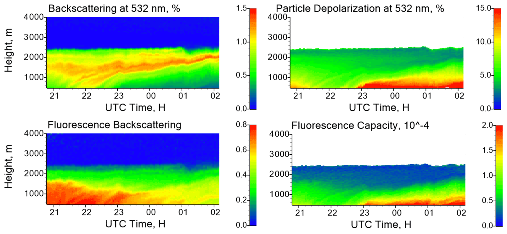
Figure 6Spatiotemporal distributions of the backscattering coefficient β532, the fluorescence backscattering coefficient βF (in 10−4 Mm−1 sr−1), the particle depolarization ratio δ532, and the fluorescence capacity GF on the night of 30–31 May 2020. The values of δ532 and GF are shown for β532 > 0.2 Mm−1 sr−1.

Figure 7(a) The δ532-GF diagram for observations in the 500–2500 m height range and (b) spatiotemporal distribution of aerosol types on the night of 30–31 May 2020. The gray coloring shows an undefined aerosol type, which is a mixture of urban and pollen for this case. Measurements with β532 < 0.2 Mm−1 sr−1 are marked in black.
The single pixel particle parameters contain statistical noise, which influences the results of the primary classification, thus producing high-frequency oscillations of nonphysical character. From a physical point of view, the aerosol single-type areas should form smooth regions, so a special smoothing procedure (stage 2 of our algorithm) was developed to remove the oscillations. The smoothing procedure is based on a convolution with a Gaussian kernel, as follows:
where t and h are temporal and height coordinates. The resolution of the classification is being controlled by the parameters sT and sH, which are set as the number of temporal and height bins.
In the second stage of classification, each of these matrices is separately convoluted with the Gauss kernel Z. After the convolution, the values for each pixel (i,j) are compared. If, e.g., the dust matrix contains a maximal value at the pixel (i,j) in respect to all other matrices, then the pixel (i,j) is finally classified as dust. The choice of smoothing parameters depends on the aerosol loading and aerosol type. For the measurements inside the boundary layer, in many cases the single pixel classification (sT = 1, sH = 1) is possible, while for analysis of the weak elevated layers, the smoothing should be applied. All results presented in this study were obtained for sT = 3 and sH = 5; thus, the temporal and range resolutions of our classification procedure are estimated to be about 8 min and 60 m, respectively.
The classification approach, described in the previous section, was applied to the data of the Mie–Raman fluorescence lidar at the ATOLL platform, located on the campus of Lille University, during 2020–2021. Here we present the results of the aerosol classification for several relevant atmospheric situations to demonstrate that different aerosol types are well separated based on the δ532–GF diagram.
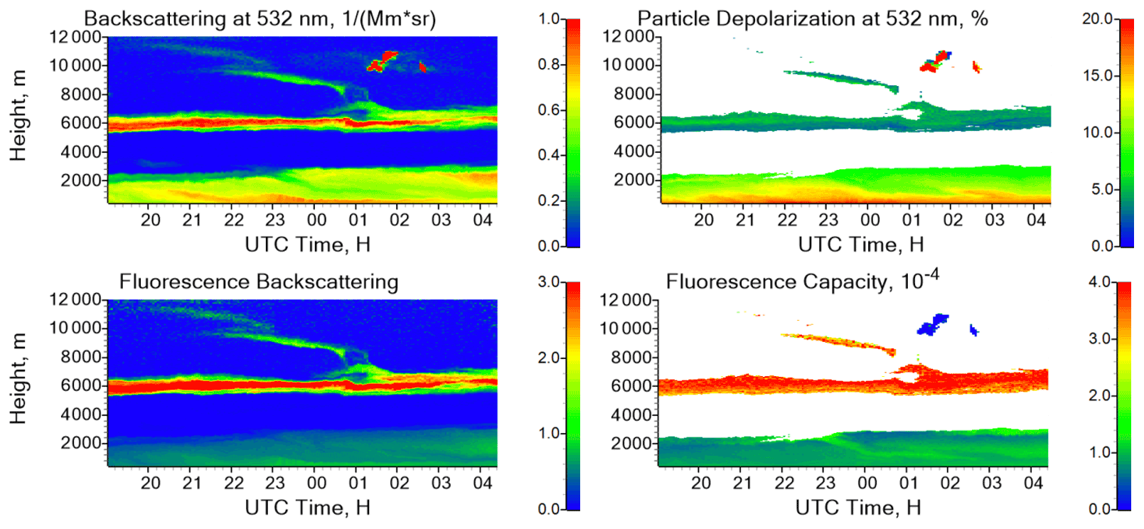
Figure 8Spatiotemporal distributions of the backscattering coefficient β532, the fluorescence backscattering coefficient βF (in 10−4 Mm−1 sr−1), the particle depolarization ratio δ532, and the fluorescence capacity GF on the night of 14–15 September 2020. The values of δ532 and GF are shown for β532 > 0.2 Mm−1 sr−1.

Figure 9(a) The δ532-GF diagram for observations in the 500–8000 m height range and (b) spatiotemporal distribution of aerosol types on the night of 14–15 September 2020. The gray coloring shows an undefined aerosol type, which is a mixture of pollen, urban, and smoke particles. Measurements with β532 < 0.2 Mm−1 sr−1 are marked in black.
4.1 12 September 2020: wildfire smoke
Figure 4 presents the spatiotemporal variations in aerosol and fluorescence backscattering coefficients (β532 and βF), together with the particle depolarization ratio δ532 and the fluorescence capacity GF, during the smoke episode on the night of 12–13 September 2020. The smoke layer extends from approximately 2 to 5 km in height, and it is characterized by a high fluorescence capacity GF > 3.0 × 10⁻⁴ and low depolarization ratio δ532 < 7 %. The cirrus clouds occurred above 11 km height during the whole night. The smoke layer was transported from North America; detailed analysis of the layer origin and transportation is given in a recent publication of Hu et al. (2022). The results of the aerosol classification for this episode are shown in Fig. 5. On the δ532-GF diagram, these data form two clusters. The first cluster includes points in the range 2.0 × 10⁻⁴ < GF < 6.0 × 10⁻⁴ and 2 % < δ532 < 7 %, and such a high fluorescence and low depolarization should be attributed to smoke particles. The second cluster consists of points localized inside 0.1 × 10⁻⁴ < GF < 0.8 × 10⁻⁴ and 1 % < δ532 < 3 % intervals, which corresponds to the urban particles in Table 1. After cluster localization, the observations can be plotted as aerosol types, using the parameters in Table 1 and the approach described in Sect. 3.2. The aerosol types in Fig. 5b are spatially separated and contain no high-frequency oscillations. Urban particles are localized at low heights, below 1 km. We would like to remind the reader that, under the condition of high relative humidity (RH), the fluorescence capacity can decrease due to the particle's hygroscopic growth. The water uptake increases the particle backscattering but does not change the fluorescence. As a result, the fluorescence capacity decreases (Veselovskii et al., 2020b). In accordance with radiosonde data, the relative humidity below 1 km was quite high (about 70 % at 500 m) and decreased with height, which can explain the wide range in the GF variation observed for urban particles in Fig. 5a.
Table 2Intensive particle parameters, such as the lidar ratios (S355, S532), particle depolarization ratios (δ355, δ532, δ1064), extinction (), and backscattering (, ) Ångström exponents for six episodes are analyzed in this work. The parameters are given for chosen height–temporal intervals, and the types of aerosol are determined from fluorescence measurements.
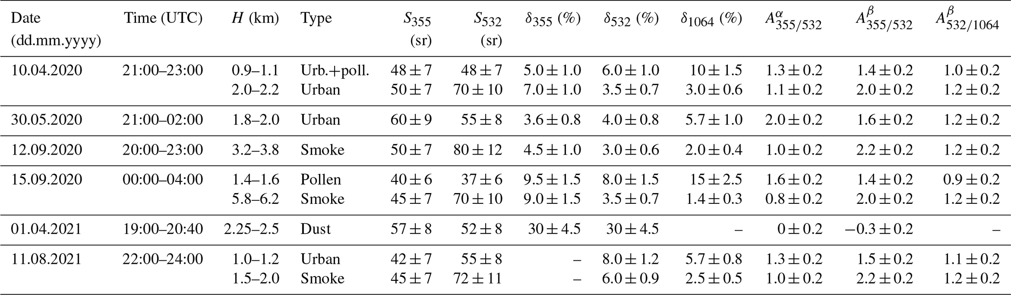
The particle intensive properties, such as the lidar ratios at 355 nm and 532 nm wavelengths (S355, S532), the particle depolarization ratios (δ355, δ532, δ1064), the extinction (), and the backscattering (, ) Ångström exponents for the episodes analyzed in this study, are summarized in Table 2. For this measurement session, in the smoke layer, the lidar ratio at 532 nm significantly exceeds the corresponding value at 355 nm (S532 = 80 ± 12 sr and S355 = 50 ± 7 sr). The particle depolarization ratio decreases with wavelength from 4.5 % at 355 nm to 2 % at 1064 nm. Such a spectral dependence of the lidar ratio and depolarization ratio for the aged smoke is in agreement with previous studies (e.g., Haarig et al., 2018; Hu et al., 2022, and references therein).
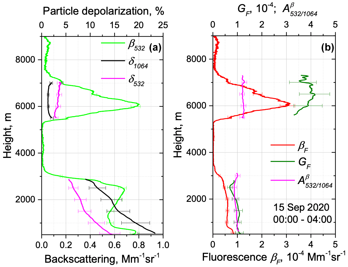
Figure 10Vertical profiles of (a) backscattering coefficient β532 and particle depolarization ratios δ532 and δ1064. (b) Fluorescence backscattering βF, fluorescence capacity GF, and backscattering Ångström exponent on 15 September 2020 for the period 00:00–04:00 UTC.
4.2 30 May 2020: urban vs. pollen
Pollen grains represent a significant fraction of primary biological materials in the troposphere, and a fluorescence-induced emission provides an opportunity for their identification. Figure 6 presents the spatiotemporal variations of β532, βF, δ532, and GF during the pollen season on the night of 30–31 May 2020. The presence of different types of pollen over Lille in spring–summer 2020 was discussed in our recent publication (Veselovskii et al., 2021). In particular, on 30 May 2020, the in situ measurements on the roof of the building demonstrate the presence of a significant amount of grass pollen. The transport of pollen can be analyzed with a global scale to mesoscale dispersion model, SILAM (Sofiev et al., 2015). In the Appendix, we show the maps of the pollen index for four sessions from this study at 22:00 UTC. On 30 May, the pollen index in the Lille region is about 5.0, indicating a high content of pollen.
Figure 11Spatiotemporal distributions of the backscattering coefficient β532, the fluorescence backscattering coefficient βF (in 10−4 Mm−1 sr−1), the particle depolarization ratio δ532, and the fluorescence capacity GF on the night of 10–11 April 2020. Measurements are performed at an angle of 45∘ to the horizon. The values of δ532 and GF are shown for β532 > 0.2 Mm−1 sr−1.

Figure 12(a) The δ532-GF diagram for observations at 350–1500 m (blue symbols) and 1500–2500 m (pink symbols) height ranges. (b) Spatiotemporal distribution of aerosol types on the night of 10–11 April 2020. The gray coloring shows an undefined aerosol type, which is a mixture of urban and pollen for this case. Measurements with β532 < 0.2 Mm−1 sr−1 are marked in black.
The aerosol is located inside the planetary boundary layer (PBL) below 2.5 km. At altitudes below 1 km, the depolarization ratio δ532 after 23:00 UTC increases up to ∼ 15 % simultaneously, with an increase in the fluorescence capacity up to 2.0 × 10⁻⁴, which can be an indication of pollen presence. In the δ532-GF diagram in Fig. 7a, the single pixel data points spread from the values typical for the urban particles to the values typical for the pollen. The contribution of pollen to the total backscattering changes with height, and the points form the pattern, similar to a characteristic curve, calculated for urban–pollen mixture in Fig. 3. In accordance with radiosonde data from the Herstmonceux station, the RH at midnight was about 40 % at 500 m, and it increased up to 70 % at 2000 m; thus, the spatiotemporal variations in RH could influence the observed values of the backscattering coefficient and depolarization ratio. In particular, the hygroscopic growth can decrease the values of both δ532 andGF. However, the value of the fluorescence capacity in Fig. 7a changes for almost 1 order of magnitude, and such a strong change in GF cannot be explained by the particle hygroscopic growth only. For example, from the recent publication of Sicard et al. (2022), an increase of β532 in urban aerosol for this range of RH is below a factor of 1.5. Thus, we suppose that the pattern in Fig. 7a is due to the mixing of the urban and pollen particles. The spatiotemporal distribution of aerosol types is shown in Fig. 7b. The urban particles (brown) are predominant, while pollen (yellow) is localized below 1 km in height. The gray color corresponds to an unidentified aerosol type which, in our case, is the mixture of urban particles and pollen.
An indicator of pollen presence in an aerosol mixture, along with a high depolarization ratio, can be a higher value of δ1064 with respect to δ532 or δ355 (Cao et al., 2010; Veselovskii et al., 2021). Vertical profiles of the particle depolarization ratio at all three wavelengths for this episode are given in Fig. 8c of Veselovskii et al. (2021). At 0.75 km height, where δ1064 is about 15 %, the ratio is 1.5, which corroborates the suggestions about pollen presence. For urban aerosol, the depolarization spectral ratio can also be above 1.0 (Burton et al., 2013), but the absolute values of depolarization are significantly lower than for pollen particles (below 10 %).
4.3 14 September 2020: wildfire smoke vs. pollen mixture
Another strong smoke episode occurred on the night of 14–15 September 2020, and the corresponding distributions of β532, βF, δ532, and GF are shown Fig. 8. The elevated smoke layer with a low depolarization ratio (δ532 < 5 %) and high fluorescence capacity (up to 4.0 × 10⁻⁴) was observed at approximately 6 km height during the whole night. Inside the boundary layer, the depolarization ratio is higher, up to 15 %, while the fluorescence capacity is lower (about 1.0 × 10⁻⁴) compared to the elevated layer. In the δ532-GF diagram in Fig. 9a, we can see the cluster of data points corresponding to the smoke. At the same time, a part of the points are inside the range of parameters attributed to the pollen (Table 1). The remaining points should be attributed to the mixture of pollen, smoke, and urban aerosol. The distribution of the particle types (Fig. 9b) of this mixture is marked with gray. The pollen particles are localized below 1 km. The presence of pollen over Lille in September is not common, but it can be transported from other regions. The SILAM pollen index in Fig. A1 for this date demonstrates the transport of pollen to northern France from the southeast of France and the eastern Mediterranean.
Figure 10a presents the profiles of δ532 and δ1064, together with β532, for the temporal interval of 00:00–04:00 UTC. The relative humidity, in accordance with radiosonde data from Herstmonceux station, did not exceed 50 % below 1.7 km. Above that height, RH increased up to 75 % at 2.5 km; thus, the observed increase of β532 above 1.5 km can be partly related to RH growth. The relative humidity inside the smoke layer did not exceed 10 %. Similar to Fig. 8, δ1064 exceeds δ532 at low heights. The ratio is about 1.5 at 1 km and inside the smoke layer 0.4. Higher values of the depolarization ratio at 532 nm compared to 1064 nm are reported for aged smoke by Haarig at al. (2018) and Hu et al. (2019, 2022). The BAE does not present significant height variations because is about 1.0 inside the PBL, and it increases to 1.25 inside the smoke layer (Fig. 10b). Simultaneously, the fluorescence capacity in the smoke layer increases about a factor of 4, compared to the PBL, which demonstrates the efficiency of the fluorescence technique for discriminating the smoke from other aerosol types.
4.4 10 April 2020: urban vs. pollen
At the beginning of April, we experienced several atmospheric situations for which elevated layers were classified as urban aerosols. One of these cases, on the night of 10–11 April 2020, is shown in Fig. 11. Lidar observations were performed at an angle of 45∘ to the horizon, so the minimum height reachable in the analysis is 350 m. The relative humidity, in accordance with radiosonde data from Herstmonceux station, increased with height from 54 % at 1.0 km to 65 % at 2.2 km. The layer with depolarization ratio δ532 below 5 % was observed at about 2 km height during the night. The fluorescence capacity in the layer is low (below 0.5 × 10⁻⁴), so it is identified as urban aerosol. HYSPLIT (Hybrid Single-Particle Lagrangian Integrated Trajectory model) backward trajectories (not shown) indicate that the air masses at 750 and 2000 m heights were transported from England (HYSPLIT, 2022). For the period 21:00–23:00 UTC, the depolarization ratio below 500 m increased simultaneously with the fluorescence capacity, which can be an indication of pollen presence.
In the δ532–GF diagram (Fig. 12a), the single pixel measurements at 350–1500 and 1500–2500 m height ranges are shown by different colors. The data points related to the upper layer are within the range of parameters expected for urban aerosol. The points in the lower layer (below 1500 m) are partly out of this range, so the aerosol type for these points is undefined. We assume that this is the mixture of urban and pollen particles because we observe particles with high depolarization (δ532 > 15 %) and fluorescence capacity up to 0.7 × 10⁻⁴. This mixture is marked in gray on the aerosol mask in Fig. 12b. The pollen index provided by SILAM over Lille at midnight is above 4.0, so the presence of pollen particles is expected.
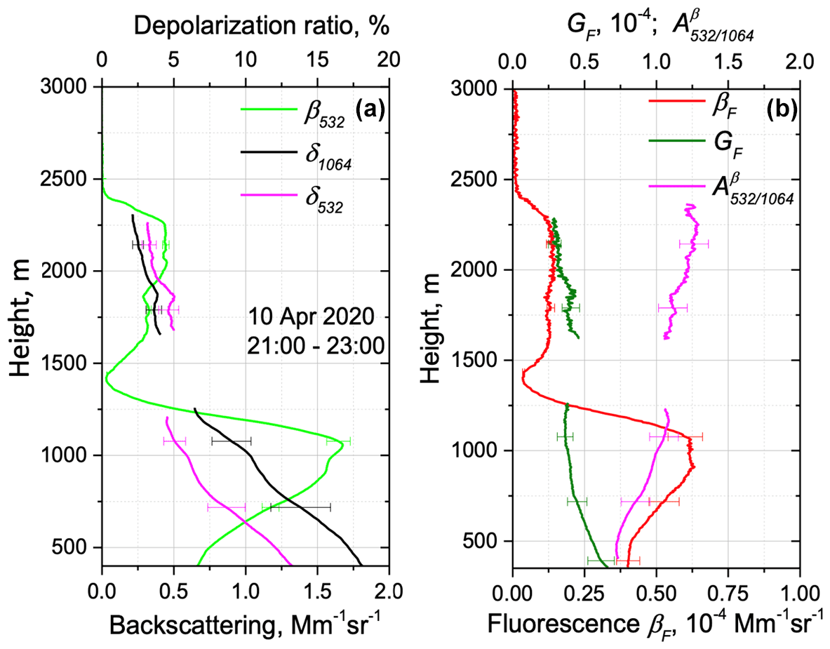
Figure 13Vertical profiles of the (a) backscattering coefficient β532 and particle depolarization ratios δ532 and δ1064. (b) Fluorescence backscattering βF, fluorescence capacity GF, and backscattering Ångström exponent on 10 April 2020 for the period 21:00–23:00 UTC.
The presence of pollen is also supported by the profiles of δ532 and δ1064, as shown in Fig. 13. At low heights, δ1064 exceeds δ532, and the ratio is about 1.4 at 0.5 km. However, inside the elevated layer, this ratio decreases and becomes about 0.8 at 2.25 km, which indicates that the mixture composition has changed. For the same height range, the fluorescence capacity decreases from 0.6 × 10⁻⁴ to 0.3 × 10⁻⁴, while gradually increases from 0.75 to 1.25, which can be due to a decrease in pollen contribution.
Figure 14Spatiotemporal distributions of the backscattering coefficient β532, the fluorescence backscattering coefficient βF (in 10−4 Mm−1 sr−1), the particle depolarization ratio δ532, and the fluorescence capacity GF on the night of 11–12 August 2021. The values of δ532 and GF are shown for β532 > 0.3 Mm−1 sr−1.
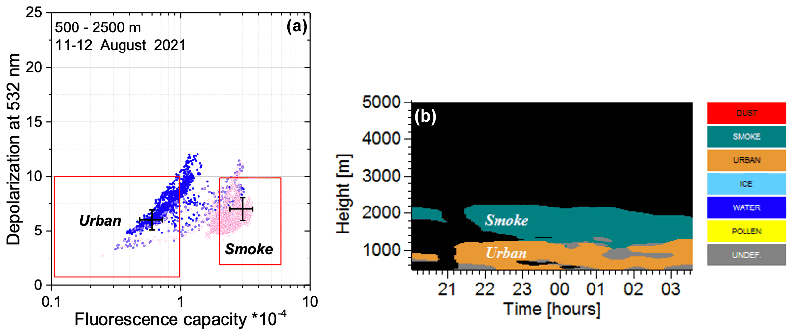
Figure 15(a) The δ532-GF diagram for observations in the 500–1400 m (blue symbols) and 1400–2500 m (pink symbols) height ranges. (b) Spatiotemporal distribution of aerosol types on the night of 11–12 August 2021. Measurements with β532 < 0.3 Mm−1 sr−1 are marked in black.
As follows from Table 2, in the lower layer, the values of S355 and S532 are close (about 48 ± 7 sr). However, in the elevated layer, S532 increases to 70 ± 7 sr, while S355 remains the same. Higher values of S532, with respect to S355, are typical for aged smoke (e.g., Müller et al., 2005; Hu et al., 2022). Moreover, significantly exceeds , which was also reported for aged smoke. Thus, based on intensive properties only, we could classify this layer as smoke. However, due to a low fluorescence capacity, in our approach, we identify it as urban.
4.5 11 August 2021: contacting layers of smoke and urban aerosol
Separation of smoke and urban particles is a challenging task for Mie–Raman lidar because both types have a small effective radius and similar depolarization ratios δ532. However, the fluorescence capacity of smoke is about a factor of 4–5 higher than that of urban aerosol, which allows their reliable separation. The analyses of the measurements on the night of 11–12 August 2021 are shown in Fig. 14. The RH decreases with height from 70 % to 40 % inside the 500–2250 m range. The main part of aerosol is concentrated below 2500 m, and two height intervals can be distinguished. Above approximately 1500 m, the layer with high fluorescence capacity (up to 3.0 × 10⁻⁴) is observed, while in the layer below 1500 m, the GF is low (below 0.8 × 10⁻⁴). HYSPLIT backward trajectories (not shown) indicate that the air masses at 1800 m heights were transported from North America, so these may contain wildfire smoke.
In the δ532-GF diagram (Fig. 15a), the single pixel measurements in the 500–1400 and 1400–2500 m height ranges are shown by different colors. The cluster of points, corresponding to the upper layer, is localized mainly inside the interval 1.8 × 10⁻⁴ < GF < 4.0 × 10⁻⁴ and 4 % < δ532 < 10 % and can be attributed to smoke. The points corresponding to the lower layer are partly identified as urban particles, but a part of the points is out of the range and forms a pattern typical for urban–pollen mixture. The SILAM pollen index in Fig. A1 is above 5.0, so the contribution of pollen can be noticeable. The smoke and urban layers are in contact and the particle mixing occurs, which increases dispersion within the clusters.
Vertical profiles of δ532 and in Fig. 16 do not demonstrate significant differences for the upper and lower layers. Meanwhile, the fluorescence capacity increases by factor of 4. The lidar ratios S355 and S532 in the upper layer, as follows from Table 2, are 45 ± 7 and 72 ± 11 sr, respectively. The significantly exceeds (2.2 ± 0.2 and 1.0 ± 0.2, respectively), so, based on intensive parameters, the upper layer can be also identified as smoke.
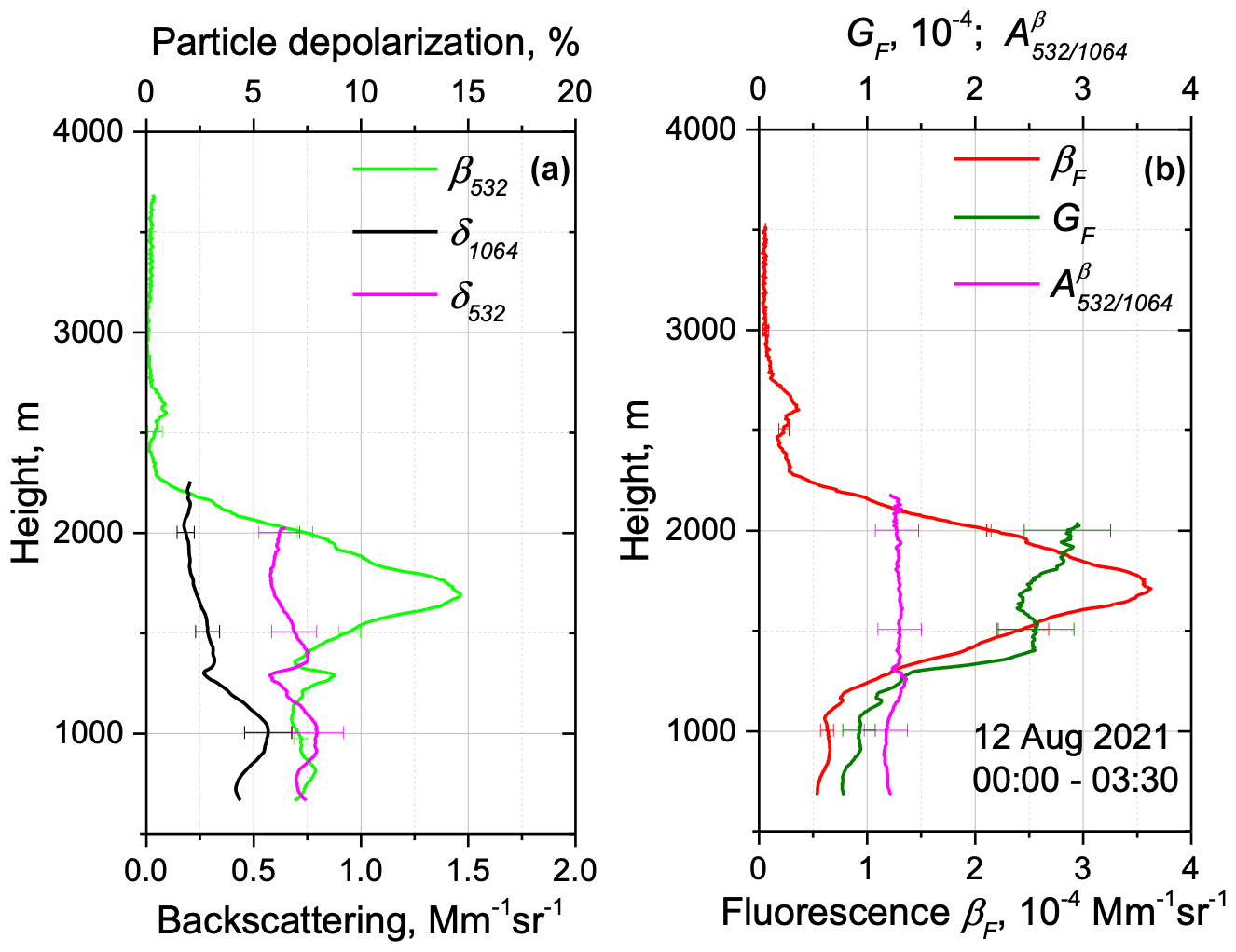
Figure 16Vertical profiles of (a) backscattering coefficient β532 and particle depolarization ratios δ532 and δ1064. (b) Fluorescence backscattering βF, fluorescence capacity GF, and backscattering Ångström exponent on 12 August 2021 for the period 00:00–03:30 UTC.
4.6 1 April 2021: dust
Dust layers transported from Africa are regularly observed over northern France. One such dust episode took place on the night of 1–2 April 2021, and the corresponding spatiotemporal variations of β532, βF, δ532, and GF are shown in Fig. 17. The dust layer, with a depolarization ratio exceeding 30 % and low fluorescence, extends from approximately 1.0 to 5.0 km in height. The fluorescence capacity varied inside the layer. In the center, it was the lowest (about 0.1 × 10⁻⁴), but at the bottom of the layer and near the top, GF increased up to (0.2–0.3) × 10−4. In Fig. 18a (δ532-GF diagram), we observe a cluster of particles which can be identified as dust. There is also a second small cluster attributed to urban aerosols. In the distribution of particle types in Fig. 18b, the urban aerosol occurs below 800 m after 23:00 UTC.

Figure 17Height–temporal distributions of the backscattering coefficient at 532 nm β532, the fluorescence backscattering coefficient βF (in 10−4 Mm−1 sr−1), the particle depolarization ratio at 532 nm δ532, and the fluorescence capacity GF on the night of 1–2 April 2021. The values of δ532 and GF are shown for β532 > 0.3 Mm−1 sr−1.

Figure 18(a) The δ532-GF diagram for observations in the 500–5000 m height range and (b) spatiotemporal distribution of aerosol types on the night of 1–2 April 2021. Measurements with β532 < 0.3 Mm−1 sr−1 are marked in black.
Figure 19 provides vertical profiles of β532, δ532, δ355, βF, GF, and . Measurements at 1064 nm were not available for this episode. Depolarization ratios at 355 and 532 nm are close to 30 % through the layer, though, at heights below 1.5 km, there is a small enhancement of δ532 up to 34 %. The fluorescence capacity is about 0.4 × 10⁻⁴ at 1.5 km, and it decreases with height to 0.1 × 10⁻⁴ at 2.5 km. However, this decrease is not accompanied by changes in the depolarization ratio. The backscattering Ångström exponent is sensitive to the enhancement of dust absorption in UV and can be negative (Veselovskii et al., 2020a). For this episode, decreases with height (together with GF) to −0.3 at 2.5 km. Similar values of were observed during SHADOW campaign in the Western Sahara (Veselovskii et al., 2020a). Above 3.75 km, both and GF start to increase. Hence, dust properties change with height, and this change is not revealed in the δ532 profile. We should mention that, in the publication of Veselovskii et al. (2020a), the increase in the dust imaginary part in the UV range also did not lead to changes in δ532.
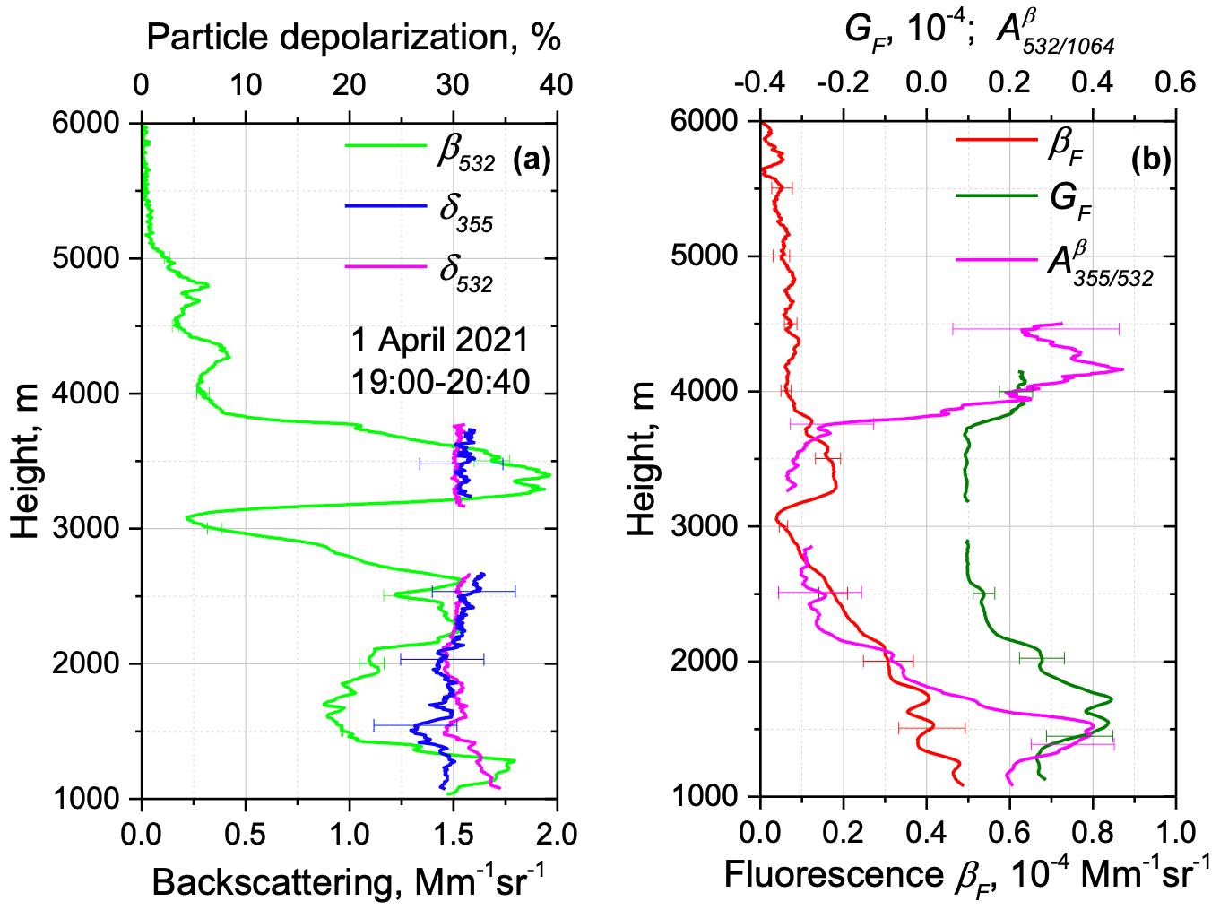
Figure 19Vertical profiles of (a) backscattering coefficient β532 and particle depolarization ratios δ532 and δ355. (b) Fluorescence backscattering βF, fluorescence capacity GF, and backscattering Ångström exponent on 1 April 2021 for the period 19:00–20:40 UTC.
The application of our new fluorescence–depolarization-based approach to the six episodes considered in this section demonstrates its ability to discriminate between several aerosol types. The first step in the validation of the results presented could be a comparison of the particle properties for obtained aerosol types with the corresponding values used in the existing classification algorithms. Table 3 provides the range of the variation in particle intensive properties from publications of Burton et al. (2013), synthetic values used in the NATALI algorithm (Nicolae et al., 2018), and parameters used in the algorithm of Papagiannopoulos et al. (2018) for the urban, smoke, and dust particles. The table contains also the range of properties variations for the episodes considered in the current study for the same aerosol types. The parameters chosen in different algorithms, even for the same aerosol type, vary in a wide range, and the values observed in this study mainly match this range of variation. We observe higher values of for urban and smoke particles, and, for dust, could be negative. Still, the values obtained in this study and the values used by other algorithms are in reasonable agreement.
Table 3Intensive particle parameters from publications of Burton et al. (2013), Nicolae et al. (2018), and Papagiannopoulos et al. (2018), together with values observed in current study for the urban, smoke, and dust particles.

The results presented in this study can be considered as the first important step in the combination of Mie–Raman and fluorescence lidar data. In the approach presented, only two intensive parameters are used for classification, i.e., the particle depolarization ratio δ532 and the fluorescence capacity GF. These parameters are chosen because they are specific for different types of aerosol and can be calculated with a high spatiotemporal resolution. Moreover, δ532 and GF can be calculated at lower altitudes compared to extinction-related parameters such as the lidar ratio and extinction Ångström exponent. Thus, classification, in principle, is possible at ranges with incomplete geometrical overlap. Finally, the computation of βF does not demand the use of a reference height, and only the calibration of relative sensitivity of the channels is needed. Thus, aerosol classification is possible, even in the presence of low-level clouds.
Though only two aerosol properties are considered, the use of fluorescence provides advances in aerosol classification. Analysis of numerous observations, performed at Lille University for the period 2020–2021, demonstrates the possibility to separate four types of aerosols, such as dust, smoke, pollen, and urban. Moreover, we are able to identify the layers containing the liquid water particles and ice. The number of determined aerosol classes can be increased by considering the particle mixtures. In particular, pure dust can be considered separately from the polluted one, which can be discriminated by lower values of the depolarization ratio.
The fluorescence technique is especially promising for the separation of smoke and urban particles because the fluorescence capacity of smoke is about a factor of 5 higher. The important advantage of fluorescence measurements is the ability to identify the biological particles in the atmosphere, such as pollen, which are usually not included in the classification schemes based on Mie–Raman observations. At the same time, our observations demonstrate that biological particles are frequently observed during spring–autumn seasons and may contribute significantly to the aerosol composition inside the PBL. The developed approach allows us to identify aerosol types with high spatiotemporal resolutions, which is estimated to be 60 m for height and less than 10 min for time, for the current instrumental configuration. Such a resolution provides an opportunity for investigating the dynamics of aerosol mixing in the troposphere.
The next step in the algorithm development will be to include additional particle properties. We plan to include the backscattering Ångström exponents and the depolarization spectral ratios ( and ), which can be also calculated with high spatiotemporal resolutions. The fluorescence capacity depends on the relative humidity, due to the effects of hygroscopic growth. Thus, information about the spatiotemporal distribution of RH should be included in the analysis. It is also important to combine our algorithm with existing classification schemes, which we plan to consider in the near future.
The SILAM is a chemical transport model developed by the Finnish Meteorological Institute (Sofiev et al., 2015). It provides information on the atmospheric composition, air quality, and pollen. In the pollen module of SILAM, six pollen types (alder, birch, grass, mugwort, olive, and ragweed) are considered. The pollen index is defined as a quantitative measure of the severity of the pollen season and a proxy of the allergenic exposure (Sofiev et al., 2012; Sofiev, 2017). The higher the pollen index is, the more pollen grains are in the atmosphere and the higher the allergy risk. Figure A1 shows the maps of pollen index in four cases. According to the description of SILAM model, the pollen index is labeled as very high when its value is greater than 4.0.
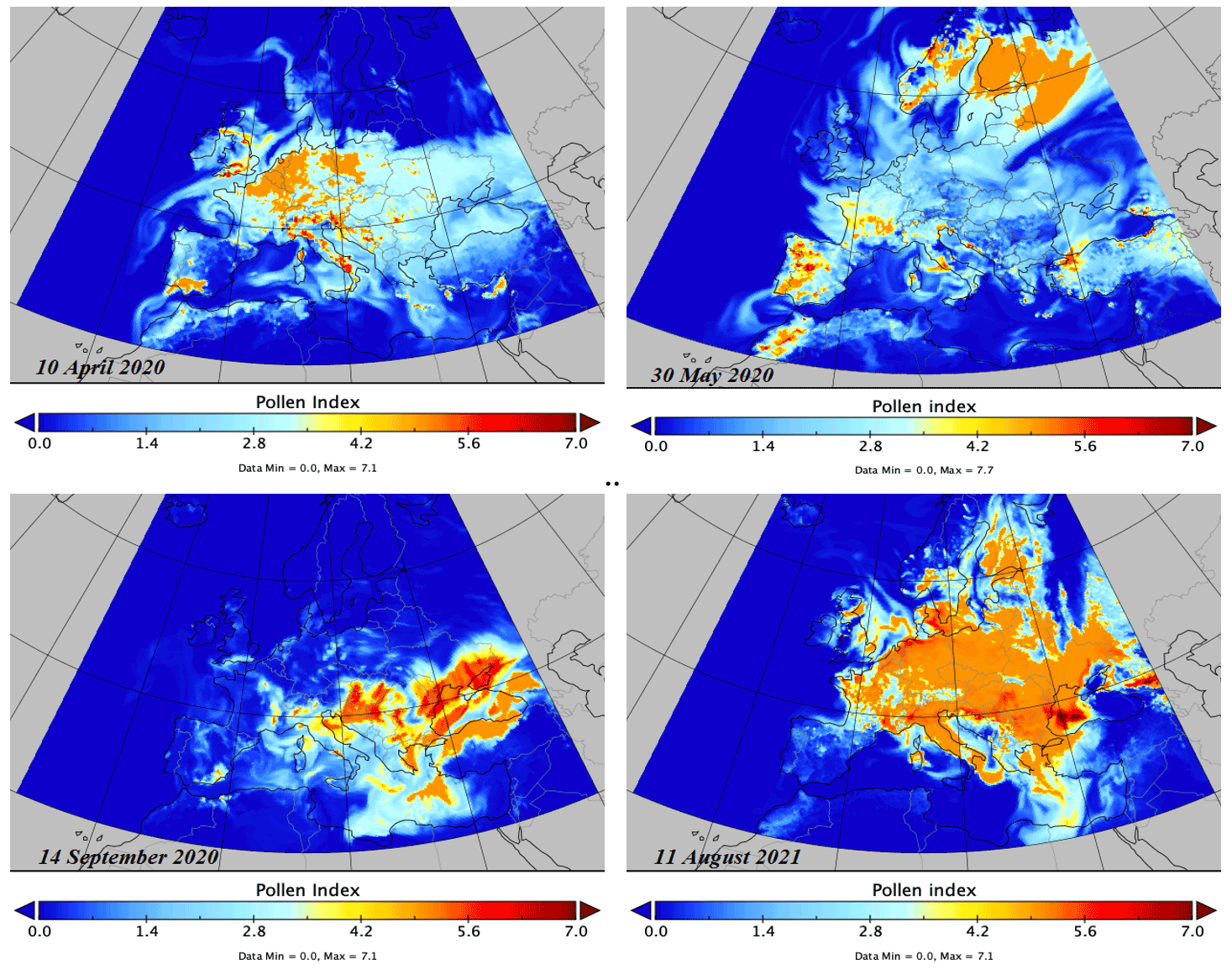
Figure A1Pollen index provided by SILAM for 10 April 2020, 30 May 2020, 14 September 2020, and 11 August 2021. The levels of pollen index are very low (< 1.0), low (1.0–2.0), moderate (2.0–3.0), high (3.0–4.0), and very high (> 4.0).
Lidar measurements are available upon request (philippe.goloub@univ-lille.fr).
IV processed the data and wrote the paper. QH and TP performed the measurements. PG supervised the project and helped with the paper preparation. BB prepared the algorithm for aerosol classification. MK developed the software for data processing.
The contact author has declared that none of the authors has any competing interests.
Publisher's note: Copernicus Publications remains neutral with regard to jurisdictional claims in published maps and institutional affiliations.
We acknowledge funding from the CaPPA project, funded by the ANR through the PIA (contract no. ANR-11-LABX-0005-01), the “Hauts de France” Regional Council (project CLIMIBIO), and the European Regional Development Fund (FEDER). The ESA/QA4EO program is greatly acknowledged, for supporting the observation activity at LOA and the OBS4CLIM Equipex project funded by ANR. Development of the algorithm for aerosol classification was supported by the Russian Science Foundation (project 21-17-00114). The SILAM model is acknowledged, for providing pollen simulations.
This research has been supported by the Centre National de la Recherche Scientifique (grant no. ANR-11-LABX-0005-01), the “Hauts de France” Regional Council (project CLIMIBIO), the European Regional Development Fund (FEDER) and the Russian Science Foundation (project 21-17-00114).
Publisher's note: the article processing charges for this publication were not paid by a Russian or Belarusian institution.
This paper was edited by Daniel Perez-Ramirez and reviewed by two anonymous referees.
Adam, M., Stachlewska, I. S., Mona, L., Papagiannopoulos, N., Bravo-Aranda, J. A., Sicard, M., Nicolae, D. N., Belegante, L., Janicka, L., Szczepanik, D., Mylonaki, M., Papanikolaou, C.-A., Siomos, N., Voudouri, K. A., Alados-Arboledas, L., Apituley, A., Mattis, I., Chaikovsky, A., Muñoz-Porcar, C., Pietruczuk, A., Bortoli, D., Baars, H., Grigorov, I., and Peshev, Z.: Biomass burning events measured by lidars in EARLINET – Part 2: Optical properties investigation, Atmos. Chem. Phys. Discuss. [preprint], https://doi.org/10.5194/acp-2021-759, 2021.
Ansmann, A., Riebesell, M., Wandinger, U., Weitkamp, C., Voss, E., Lahmann, W., and Michaelis, W.: Combined Raman elastic-backscatter lidar for vertical profiling of moisture, aerosols extinction, backscatter, and lidar ratio, Appl. Phys. B, 55, 18–28, 1992.
Bohlmann, S., Shang, X., Giannakaki, E., Filioglou, M., Saarto, A., Romakkaniemi, S., and Komppula, M.: Detection and characterization of birch pollen in the atmosphere using a multiwavelength Raman polarization lidar and Hirst-type pollen sampler in Finland, Atmos. Chem. Phys., 19, 14559–14569, https://doi.org/10.5194/acp-19-14559-2019, 2019.
Boucher, O., Randall, D., Artaxo, P., Bretherton, C., Feingold, G., Forster, P., Kerminen, V.-M., Kondo, Y., Liao, H., Lohmann, U., Rasch, P., Satheesh, S. K., Sherwood, S., Stevens, B., and Zhang, X. Y.: Clouds and Aerosols, in: Climate Change 2013: The Physical Science Basis. Contribution of Working Group I to the Fifth Assessment Report of the Intergovernmental Panel on Climate Change, edited by: Stocker, T. F., Qin, D., Plattner, G.-K., Tignor, M., Allen, S. K., Boschung, J., Nauels, A., Xia, Y., Bex, V., and Midgley, P., M., Cambridge University Press, Cambridge, United Kingdom and New York, NY, USA, ISBN 978-1-107-05799-1, 2013.
Burton, S. P., Ferrare, R. A., Hostetler, C. A., Hair, J. W., Rogers, R. R., Obland, M. D., Butler, C. F., Cook, A. L., Harper, D. B., and Froyd, K. D.: Aerosol classification using airborne High Spectral Resolution Lidar measurements – methodology and examples, Atmos. Meas. Tech., 5, 73–98, https://doi.org/10.5194/amt-5-73-2012, 2012.
Burton, S. P., Ferrare, R. A., Vaughan, M. A., Omar, A. H., Rogers, R. R., Hostetler, C. A., and Hair, J. W.: Aerosol classification from airborne HSRL and comparisons with the CALIPSO vertical feature mask, Atmos. Meas. Tech., 6, 1397–1412, https://doi.org/10.5194/amt-6-1397-2013, 2013.
Burton, S. P., Vaughan, M. A., Ferrare, R. A., and Hostetler, C. A.: Separating mixtures of aerosol types in airborne High Spectral Resolution Lidar data, Atmos. Meas. Tech., 7, 419–436, https://doi.org/10.5194/amt-7-419-2014, 2014.
Burton, S. P., Hair, J. W., Kahnert, M., Ferrare, R. A., Hostetler, C. A., Cook, A. L., Harper, D. B., Berkoff, T. A., Seaman, S. T., Collins, J. E., Fenn, M. A., and Rogers, R. R.: Observations of the spectral dependence of linear particle depolarization ratio of aerosols using NASA Langley airborne High Spectral Resolution Lidar, Atmos. Chem. Phys., 15, 13453–13473, https://doi.org/10.5194/acp-15-13453-2015, 2015.
Cao, X., Roy, G., and Bernier, R.: Lidar polarization discrimination of bioaerosols, Opt. Eng., 49, 116201, https://doi.org/10.1117/1.3505877, 2010.
Dubovik, O., Holben, B. N., Eck, T. F., Smirnov, A., Kaufman, Y. J., King, M. D., Tanre, D., and Slutsker, I.: Variability of absorption and optical properties of key aerosol types observed in worldwide locations, J. Atmos. Sci., 59, 590–608, 2002.
Freudenthaler, V., Esselborn, M., Wiegner, M., Heese, B., Tesche, M., Ansmann, A., Müller, D., Althausen, D., Wirth, M., Fix, A., Ehret, G., Knippertz, P., Toledano, C., Gasteiger, J., Garhammer, M., and Seefeldner, M.: Depolarization ratio profiling at several wavelengths in pure Saharan dust during SAMUM 2006, Tellus, 61B, 165–179, 2009.
Gasteiger, J. and Freudenthaler, V.: Benefit of depolarization ratio at λ=1064 nm for the retrieval of the aerosol microphysics from lidar measurements, Atmos. Meas. Tech., 7, 3773–3781, https://doi.org/10.5194/amt-7-3773-2014, 2014.
Giles, D. M., Holben, B. N., Eck, T. F., Sinyuk, A., Smirnov, A., Slutsker, I., Dickerson, R. R., Thompson, A. M., and Schafer, J. S.: An analysis of AERONET aerosol absorption properties and classifications representative of aerosol source regions, J. Geophys. Res. 117, D17203, https://doi.org/10.1029/2012JD018127, 2012.
Groß, S., Tesche, M., Freudenthaler, V., Toledano, C., Wiegner, M., Ansmann, A., Althausen D., and Seefeldner, M.: Characterization of Saharan dust, marine aerosols and mixtures of biomass-burning aerosols and dust by means of multi-wavelength depolarization and Raman lidar measurements during SAMUM 2, Tellus B, 63, 706–724, https://doi.org/10.1111/j.1600-0889.2011.00556.x, 2011.
Groß, S., Esselborn, M., Weinzierl, B., Wirth, M., Fix, A., and Petzold, A.: Aerosol classification by airborne high spectral resolution lidar observations, Atmos. Chem. Phys., 13, 2487–2505, https://doi.org/10.5194/acp-13-2487-2013, 2013.
Haarig, M., Ansmann, A., Baars, H., Jimenez, C., Veselovskii, I., Engelmann, R., and Althausen, D.: Depolarization and lidar ratios at 355, 532, and 1064 nm and microphysical properties of aged tropospheric and stratospheric Canadian wildfire smoke, Atmos. Chem. Phys., 18, 11847–11861, https://doi.org/10.5194/acp-18-11847-2018, 2018.
Hamill, P., Giordano, M., Ward, C., Giles, D., and Holben, B.: An AERONET-based aerosol classification using the Mahalanobis distance, Atmos. Environ., 140, 213–233, https://doi.org/10.1016/j.atmosenv.2016.06.002, 2016.
Hara, Y., Nishizawa, T., Sugimoto, N., Osada, K., Yumimoto, K., Uno, I., Kudo, R., and Ishimoto, H.: Retrieval of aerosol components using multi-wavelength Mie-Raman lidar and comparison with ground aerosol sampling, Remote Sens., 10, 937. https://doi.org/10.3390/rs10060937, 2018.
Hu, Q., Goloub, P., Veselovskii, I., Bravo-Aranda, J.-A., Popovici, I. E., Podvin, T., Haeffelin, M., Lopatin, A., Dubovik, O., Pietras, C., Huang, X., Torres, B., and Chen, C.: Long-range-transported Canadian smoke plumes in the lower stratosphere over northern France, Atmos. Chem. Phys., 19, 1173–1193, https://doi.org/10.5194/acp-19-1173-2019, 2019.
Hu, Q., Goloub, P., Veselovskii, I., and Podvin, T.: The characterization of long-range transported North American biomass burning plumes: what can a multi-wavelength Mie–Raman-polarization-fluorescence lidar provide?, Atmos. Chem. Phys., 22, 5399–5414, https://doi.org/10.5194/acp-22-5399-2022, 2022.
HYSPLIT: HYbrid Single-Particle Lagrangian Integrated Trajectory model, backward trajectory calculation tool, http://ready.arl.noaa.gov/HYSPLIT_traj.php, last access: 14 June 2022.
Klett, J. D.: Lidar inversion with variable backscatter/extinction ratios, Appl. Opt., 24, 1638–1643, 1985.
Li, L., Dubovik, O., Derimian, Y., Schuster, G. L., Lapyonok, T., Litvinov, P., Ducos, F., Fuertes, D., Chen, C., Li, Z., Lopatin, A., Torres, B., and Che, H.: Retrieval of aerosol components directly from satellite and ground-based measurements, Atmos. Chem. Phys., 19, 13409–13443, https://doi.org/10.5194/acp-19-13409-2019, 2019.
Mamouri, R.-E. and Ansmann, A.: Potential of polarization/Raman lidar to separate fine dust, coarse dust, maritime, and anthropogenic aerosol profiles, Atmos. Meas. Tech., 10, 3403–3427, https://doi.org/10.5194/amt-10-3403-2017, 2017.
Müller, D., Mattis, I., Wandinger, U., Ansmann, A., Althausen, A., and Stohl, A.: Raman lidar observations of aged Siberian and Canadian forest fire smoke in the free troposphere over Germany in 2003: Microphysical particle characterization, J. Geophys. Res., 110, D17201, https://doi.org/10.1029/2004JD005756, 2005.
Mylonaki, M., Giannakaki, E., Papayannis, A., Papanikolaou, C.-A., Komppula, M., Nicolae, D., Papagiannopoulos, N., Amodeo, A., Baars, H., and Soupiona, O.: Aerosol type classification analysis using EARLINET multiwavelength and depolarization lidar observations, Atmos. Chem. Phys., 21, 2211–2227, https://doi.org/10.5194/acp-21-2211-2021, 2021.
Nicolae, D., Vasilescu, J., Talianu, C., Binietoglou, I., Nicolae, V., Andrei, S., and Antonescu, B.: A neural network aerosol-typing algorithm based on lidar data, Atmos. Chem. Phys., 18, 14511–14537, https://doi.org/10.5194/acp-18-14511-2018, 2018.
Papagiannopoulos, N., Mona, L., Amodeo, A., D'Amico, G., Gumà Claramunt, P., Pappalardo, G., Alados-Arboledas, L., Guerrero-Rascado, J. L., Amiridis, V., Kokkalis, P., Apituley, A., Baars, H., Schwarz, A., Wandinger, U., Binietoglou, I., Nicolae, D., Bortoli, D., Comerón, A., Rodríguez-Gómez, A., Sicard, M., Papayannis, A., and Wiegner, M.: An automatic observation-based aerosol typing method for EARLINET, Atmos. Chem. Phys., 18, 15879–15901, https://doi.org/10.5194/acp-18-15879-2018, 2018.
Pappalardo, G., Amodeo, A., Apituley, A., Comeron, A., Freudenthaler, V., Linné, H., Ansmann, A., Bösenberg, J., D'Amico, G., Mattis, I., Mona, L., Wandinger, U., Amiridis, V., Alados-Arboledas, L., Nicolae, D., and Wiegner, M.: EARLINET: towards an advanced sustainable European aerosol lidar network, Atmos. Meas. Tech., 7, 2389–2409, https://doi.org/10.5194/amt-7-2389-2014, 2014.
Reichardt, J.: Cloud and aerosol spectroscopy with Raman lidar, J. Atmos. Ocean. Tech., 31, 1946–1963, https://doi.org/10.1175/JTECH-D-13-00188.1, 2014.
Reichardt, J., Leinweber, R., and Schwebe, A.: Fluorescing aerosols and clouds: investigations of co-existence, Proceedings of the 28th ILRC, 25–30 June 2017, Bucharest, Romania, EPJ Web of Conferences, 176, 05010, https://doi.org/10.1051/epjconf/201817605010, 2018.
Rittmeister, F., Ansmann, A., Engelmann, R., Skupin, A., Baars, H., Kanitz, T., and Kinne, S.: Profiling of Saharan dust from the Caribbean to western Africa – Part 1: Layering structures and optical properties from shipborne polarization/Raman lidar observations, Atmos. Chem. Phys., 17, 12963–12983, https://doi.org/10.5194/acp-17-12963-2017, 2017.
Saito, Y., Hosokawa, T., and Shiraishi, K.: Collection of excitation-emission-matrix fluorescence of aerosol-candidate-substances and its application to fluorescence lidar monitoring, Appl. Opt., 61, 653–660, 2022.
Schuster, G. L., Dubovik, O., and Arola, A.: Remote sensing of soot carbon – Part 1: Distinguishing different absorbing aerosol species, Atmos. Chem. Phys., 16, 1565–1585, https://doi.org/10.5194/acp-16-1565-2016, 2016.
Sicard, M., Fortunato dos Santos Oliveira, D. C., Muñoz-Porcar, C., Gil-Díaz, C., Comerón, A., Rodríguez-Gómez, A., and Dios Otín, F.: Measurement report: Spectral and statistical analysis of aerosol hygroscopic growth from multi-wavelength lidar measurements in Barcelona, Spain, Atmos. Chem. Phys., 22, 7681–7697, https://doi.org/10.5194/acp-22-7681-2022, 2022.
Sofiev, M.: On impact of transport conditions on variability of the seasonal pollen index, Aerobiologia, 33, 167–179, https://doi.org/10.1007/s10453-016-9459-x, 2017.
Sofiev, M., Siljamo, P., Ranta, H., Linkosalo, T., Jaeger,S., Rasmussen, A., Rantio-Lehtimaki, A., Severova, E., and Kukkonen, J.: A numerical model of birch pollen emission and dispersion in the atmosphere. Description of the emission module, Int. J. Biometeorol., 57, 45–58, https://doi.org/10.1007/s00484-012-0532-z, 2012.
Sofiev, M., Vira, J., Kouznetsov, R., Prank, M., Soares, J., and Genikhovich, E.: Construction of the SILAM Eulerian atmospheric dispersion model based on the advection algorithm of Michael Galperin, Geosci. Model Dev., 8, 3497–3522, https://doi.org/10.5194/gmd-8-3497-2015, 2015.
Sugimoto, N. and Lee, C. H.: Characteristics of dust aerosols inferred from lidar depolarization measurements at two wavelengths, Appl. Opt., 45, 7468–7474, https://doi.org/10.1364/AO.45.007468, 2006.
Sugimoto, N., Huang, Z., Nishizawa, T., Matsui, I., and Tatarov, B.: Fluorescence from atmospheric aerosols observed with a multichannel lidar spectrometer, Opt. Expr., 20, 20800–20807, 2012.
Tesche, M., Ansmann, A., Müller, D., Althausen, D., Mattis, I., Heese, B., Freudenthaler, V., Wiegner, M., Eseelborn, M., Pisani, G., and Knippertz, P.: Vertical profiling of Saharan dust with Raman lidars and airborne HSRL in southern Morocco during SAMUM, Tellus B, 61, 144–164, 2009.
Veselovskii, I., Whiteman, D. N., Korenskiy, M., Suvorina, A., and Pérez-Ramírez, D.: Use of rotational Raman measurements in multiwavelength aerosol lidar for evaluation of particle backscattering and extinction, Atmos. Meas. Tech., 8, 4111–4122, https://doi.org/10.5194/amt-8-4111-2015, 2015.
Veselovskii, I., Hu, Q., Goloub, P., Podvin, T., Korenskiy, M., Derimian, Y., Legrand, M., and Castellanos, P.: Variability in lidar-derived particle properties over West Africa due to changes in absorption: towards an understanding, Atmos. Chem. Phys., 20, 6563–6581, https://doi.org/10.5194/acp-20-6563-2020, 2020a.
Veselovskii, I., Hu, Q., Goloub, P., Podvin, T., Korenskiy, M., Pujol, O., Dubovik, O., and Lopatin, A.: Combined use of Mie–Raman and fluorescence lidar observations for improving aerosol characterization: feasibility experiment, Atmos. Meas. Tech., 13, 6691–6701, https://doi.org/10.5194/amt-13-6691-2020, 2020b.
Veselovskii, I., Hu, Q., Goloub, P., Podvin, T., Choël, M., Visez, N., and Korenskiy, M.: Mie–Raman–fluorescence lidar observations of aerosols during pollen season in the north of France, Atmos. Meas. Tech., 14, 4773–4786, https://doi.org/10.5194/amt-14-4773-2021, 2021.
Veselovskii, I., Hu, Q., Ansmann, A., Goloub, P., Podvin, T., and Korenskiy, M.: Fluorescence lidar observations of wildfire smoke inside cirrus: a contribution to smoke–cirrus interaction research, Atmos. Chem. Phys., 22, 5209–5221, https://doi.org/10.5194/acp-22-5209-2022, 2022.
Voudouri, K. A., Siomos, N., Michailidis, K., Papagiannopoulos, N., Mona, L., Cornacchia, C., Nicolae, D., and Balis, D.: Comparison of two automated aerosol typing methods and their application to an EARLINET station, Atmos. Chem. Phys., 19, 10961–10980, https://doi.org/10.5194/acp-19-10961-2019, 2019.
Wang, N., Shen, X., Xiao, D., Veselovskii, I., Zhao, C., Chen, F., Liu, C., Rong, Y., Ke, J., Wang, B., Qi, B., and Liu, D.: Development of ZJU high-spectral-resolution lidar for aerosol and cloud: feature detection and classification, J. Quant. Spectrosc. Ra., 261, 107513, https://doi.org/10.1016/j.jqsrt.2021.107513, 2021.
Whiteman, D. N.: Examination of the traditional Raman lidar technique. II. Evaluating the ratios for water vapor and aerosols, Appl. Opt., 42, 2593–2608, https://doi.org/10.1364/AO.42.002593, 2003.
Zhang, Y., Li, Z., Chen, Y., de Leeuw, G., Zhang, C., Xie, Y., and Li, K.: Improved inversion of aerosol components in the atmospheric column from remote sensing data, Atmos. Chem. Phys., 20, 12795–12811, https://doi.org/10.5194/acp-20-12795-2020, 2020.
Zhang, Y., Sun, Z., Chen, S., Chen, H., Guo, P., Chen, S., He, J., Wang, J., and Nian, X.: Classification and source analysis of low-altitude aerosols in Beijing using fluorescence–Mie polarization lidar, Opt. Commun., 479, 126417, https://doi.org/10.1016/j.optcom.2020.126417, 2021.
- Abstract
- Introduction
- Experimental setup and data analysis
- Aerosol classification based on fluorescence measurements
- Application of classification approach to LILAS data
- Conclusion
- Appendix A: Pollen index provided by SILAM
- Data availability
- Author contributions
- Competing interests
- Disclaimer
- Acknowledgements
- Financial support
- Review statement
- References