the Creative Commons Attribution 4.0 License.
the Creative Commons Attribution 4.0 License.
 | 31 Jan 2022
Calibration of radar differential reflectivity using quasi-vertical profiles
Daniel Sanchez-Rivas
Miguel A. Rico-Ramirez
Accurate precipitation estimation with weather radars is essential for hydrological and meteorological applications. The differential reflectivity (ZDR) is a crucial weather radar measurement that helps to improve quantitative precipitation estimates using polarimetric weather radars. However, a system bias between the horizontal and vertical channels generated by the radar produces an offset in ZDR. Existing methods to calibrate ZDR measurements rely on the intrinsic values of the ZDR of natural targets (e.g. drizzle or dry snow) collected at high elevation angles (e.g. higher than 40∘ or even at 90∘), in which ZDR values close to 0 dB are expected. However, not all weather radar systems can scan at such high elevation angles or point the antenna vertically to collect precipitation measurements passing overhead. Therefore, there is a need to develop new methods to calibrate ZDR measurements using lower-elevation scans. In this work, we present and analyse a novel method for correcting and monitoring the ZDR offset using quasi-vertical profiles computed from scans collected at 9∘ elevations. The method is applied to radar data collected through 1 year of precipitation events by two operational C-band polarimetric weather radars in the UK. The proposed method shows a relative error of 0.1 dB when evaluated against the traditional approach based on ZDR measurements collected at 90∘ elevations. Additionally, the method is independently assessed using disdrometers located near the radar sites. The results showed a reasonable agreement between disdrometer-derived and radar-calibrated ZDR measurements.
- Article
(7113 KB) - Full-text XML
- BibTeX
- EndNote


Conventional weather radars transmit signals in the microwave frequency range that are backscattered towards the radar antenna when precipitation particles (also known as hydrometeors, including raindrops, snow, melting snow, hail, graupel) lie along the path of the radar beam. The signal backscattered by hydrometeors is related to the radar reflectivity Z that can be converted to an estimation of rainfall rate R using a power-law equation Z=aRb. Dual-polarisation weather radars measure the radar reflectivity at horizontal ZH and vertical ZV polarisations, and the ratio between both of them is known as the differential reflectivity ZDR. ZDR was proposed to improve radar rainfall estimation because raindrops are distorted into oblate spheroids as they fall to the ground (Pruppacher and Beard, 1970; Seliga and Bringi, 1976). Small raindrops give ZDR values close to zero, whereas larger raindrops give ZDR>0. The differential reflectivity (ZDR) plays a crucial role in quantitative precipitation estimation (QPE) algorithms using polarimetric weather radars. Its relation with the orientation, shape and size of the hydrometeors improves not only the accuracy of radar QPE algorithms (Bringi et al., 2011; Cifelli et al., 2011; Giangrande and Ryzhkov, 2008; Ryzhkov et al., 2005b; Vulpiani et al., 2009) but also the classification of hydrometeors (Al-Sakka et al., 2013; Besic et al., 2016; Park et al., 2009; Straka et al., 2000).
However, to incorporate ZDR as a valid input for radar QPE, it is necessary to ensure that it is properly calibrated. Ryzhkov et al. (2005a) showed that an accuracy of 0.2 dB in the differential reflectivity calibration is desirable for practical applications of polarimetric weather radar data, as this value generates uncertainty in the rain estimates close to 18 %. However, several factors introduce a bias into ZDR, e.g. (a) the presence of cross-polar radiation (Zrnić et al., 2010); (b) errors in the transmitter and the receiver chain (or both) (Zrnic et al., 2006), or (c) an overall system bias due to the ratio of power transmitted to the horizontal and vertical polarisations (Bringi and Chandrasekar, 2001).
Several calibration procedures have been proposed to correct the overall system bias (or offset) in ZDR depending on the radar scanning strategy. For radars capable of performing measurements at a 90∘ elevation angle (herein referred to as birdbath scans), the most accepted calibration procedure is based on radar observations of raindrops as the antenna rotates about the vertical; non-zero values of ZDR present under these conditions can be set as the ZDR offset. This method was introduced by Gorgucci et al. (1999) and has been further explored and validated on several radar campaigns; e.g. Bechini et al. (2002) used vertical profiles (VPs) generated from data collected by a weather radar located in Italy to estimate both the ZDR offset and the error in the radar reflectivity (ZH). They analysed the standard deviation of ZDR taken at vertical incident and concluded that the accuracy of this method is close to 0.1 dB. Similarly, Gourley et al. (2009) estimated the ZDR offset using birdbath scans collected by a C-band radar, and their results demonstrated its impact on the absolute calibration of ZH; Louf et al. (2019) used polarimetric birdbath scans measured by a C-band radar located in Australia to validate a new approach for calibrating and monitoring ZH using ground clutter and satellite data. Frech and Hubbert (2020) used data collected from the radar network operated by the German Meteorological Service to monitor the ZDR calibration. Their method relies on range-averaged values of ZDR collected in light rain and detected using thresholds on polarimetric variables like the co-polar correlation coefficient or the coherent power to target an accuracy of ZDR of around ±0.1 dB. More recently, Ferrone and Berne (2021) expanded the birdbath method by estimating the offset based on interpolated ZDR values taken from rain, snow or ice regions, the main advantage of this method being its applicability when rain regions are not available to estimate the ZDR offset.
However, some weather radar networks are unable to perform birdbath scans due to mechanical constraints. So several procedures have been proposed to overcome this restriction and correct the ZDR offset. Ryzhkov et al. (2005a) presented a method based on the ZDR values of dry snow collected at elevation angles between 40 and 60∘. They linked these values to the ZDR offset, achieving an accuracy of 0.2 dB. Giangrande and Ryzhkov (2005) expanded this method for scans affected by the presence of partial beam blockage and explored its relation with the ZDR offset, stating that this method achieves an accuracy of 0.3 dB when applied to large data sets. Bechini et al. (2008) proposed a method to quantify the ZDR offset by probing the differential reflectivity while increasing the elevation angle but remaining below the melting layer (ML). Then these data are compared with theoretical profiles of ZDR to estimate the ZDR offset. Although it is possible to achieve high accuracy by applying this method (∼0.1 dB), thousands of profiles are needed to generate profiles suitable for the comparison process.
Another well-known technique to calibrate ZDR relies on sun measurements. It is based on the detection of solar spike echoes as this type of radiation has equal power at both horizontal and vertical polarisations (Gourley et al., 2006), hence generating measurements of ZDR close to 0 dB. The sun-radiation detection method has been further investigated in several works; e.g. Gourley et al. (2006) compared both the birdbath scans and sun-radiation detection methods using C-band polarimetric data, determining that higher accuracy is achieved when using the former. An online variation of the solar-radiation detection method that does not require the operational scanning strategy to be stopped was introduced by Holleman et al. (2010). It is based on other works conceived to monitor the absolute radar calibration, like the methods introduced by Darlington et al. (2003) and Huuskonen and Holleman (2007). This online method enables monitoring the calibration of ZDR and also the analysis of the correlation between horizontal and vertical channels. Later, Huuskonen et al. (2016) expanded this method based on data collected from the Finnish radar network, adding quality control to the solar signals and achieving accuracy of ZDR below 0.05 dB. Chu et al. (2019) also used the sun-radiation detection method and concluded that an accurate calibration depends on the availability of radar data taken at sunrise/sunset, among other considerations. It is worth noting that the offset detected by the solar method must be taken with care as it is related to the receiver chain only, whereas the offset computed from birdbath scans includes both the transmitter and the receiver chain (Huuskonen et al., 2016).
Some other alternative techniques have been proposed to complement the operational calibration and monitoring of ZDR. Bringi et al. (2006) estimated the ZDR offset using range–height–indicator (RHI) scans collected by a C-band polarimetric radar located in Japan. They probed ZDR in ice regions (i.e. at high altitudes) where values of 0 dB are expected and set the mean values of the observed data as the ZDR offset. Richardson et al. (2017) proposed the use of turbulent eddies to monitor the differential reflectivity as the nature of such scatters results in values of ZDR close to 0 dB. Additionally, Ryzhkov et al. (2016) proposed the application of the quasi-vertical profile (QVP) approach to monitor the calibration of ZDR using a similar rationale to that in Ryzhkov et al. (2005a). This approach is explored by Griffin et al. (2020) and Kumjian et al. (2016), in which previously offset-corrected QVPs of ZDR are used to describe processes like the ML and ice aggregation/riming. Although the QVPs are a valuable tool for monitoring the temporal evolution of precipitation and the microphysics of precipitation, there is little research using QVPs in rain to estimate the ZDR offset. Most of the ZDR calibration methods described above (except for the method that relies on sun measurements) rely on higher-elevation scans. There is a need to develop alternative methods that can be used when only lower-elevation scans are available.
This study presents an operational method to correct the ZDR offset that can be implemented using QVPs of polarimetric variables. The method is based on QVPs generated from scans with elevation angles of 9∘ and collected during light rain. These scans are usually available in operational radar scanning strategies deployed in radar networks worldwide, thus becoming an excellent option for radar networks not capable of collecting measurements at vertical incidence. The C-band polarimetric weather radars developed by the UK Met Office (UKMO) can perform measurements at vertical incidence, allowing a thorough comparison of the performance of both methods. Additionally, we explore the temporal variation in the ZDR offset using long-term observations collected by two operational weather radars. The calibrated ZDR measurements are further compared with measurements from independent disdrometer observations located near the radar sites. The paper is organised as follows. In Sect. 2, we define the radar and disdrometer data sets used in this work. The two different methods used to calibrate the radar ZDR are described in Sect. 3. In Sect. 4, we examine the performance of the proposed method using long-term data sets collected by two weather radars and several disdrometers. We discuss the methods and results in Sect. 5. Finally, we summarise the findings of this work in Sect. 6.
2.1 Radar data sets
The raw polarimetric radar data sets were obtained from two C-band weather radars that are part of the UKMO operational weather radar network. The Chenies radar site is located at Hertfordshire, near London, the United Kingdom (Met Office, 2013), and the Dean Hill radar site is located at Wiltshire, near Salisbury, the United Kingdom (Met Office, 2021). Both radars transmit and receive signals at horizontal and vertical polarisations simultaneously, generating plan position indicator (PPI) products at various pulse lengths and revolutions per minute (RPM) and covering several elevation angles. The PPI products include measurements of reflectivity (ZH), differential reflectivity (ZDR), the correlation coefficient (ρHV), the differential propagation phase (ΦDP) and radial velocity (V) collected throughout 2018 to carry out a long-term analysis of the ZDR calibration; such products and their processing are described next.
The birdbath scans are sampled with the radar antenna pointing vertically (i.e. 90∘ elevation angle) while at the same time the antenna rotates around its axis (from 0 to 360∘ in azimuth). The scans have a temporal resolution of 10 min, 75 m of gate resolution and a maximum range (equivalent to height for vertical scans) of 12 km. These products are used to build vertical profiles (VPs) of polarimetric variables and monitor the ZDR calibration. The VPs are generated by averaging raw polarimetric data taken from 360 vertical rays following the procedure suggested by Bechini et al. (2002); however, the first kilometre in height is discarded to minimise the risk of side-lobe contamination and the presence of other artefacts that could affect the ZDR calibration. Also, the VPs are used as input for a ML detection algorithm to distinguish the precipitation in the liquid phase, as described in Sanchez-Rivas and Rico-Ramirez (2021). These VPs will be used to compute the true ZDR calibration offset, which will be used to validate the proposed algorithm. Note that this ZDR offset is not error-free but provides a reliable benchmark to validate our algorithm.
PPI scans at a 9∘ elevation angle are collected every 10 min and sampled in short-pulse (SP) mode (pulse length equal to 500 µs), with a gate resolution of 600 m and a maximum range of 115 km. These scans are processed to generate QVPs of polarimetric variables following the procedure suggested by Ryzhkov et al. (2016), averaging azimuthally the polarimetric variables and generating one QVP of each polarimetric variable per PPI scan. As above, these data are also used to detect the ML. These QVPs will be used to calibrate and monitor ZDR using lower-elevation scans.
PPI scans at 0.5, 1.0 and 2.0∘ elevation angles are collected every 5 min and sampled in long-pulse (LP) mode (pulse length equal to 2000 µs), covering a range of 250 km and with the same gate resolution as above. These low elevation angles are used to compare the offset-corrected radar ZDR with ZDR values derived from disdrometer data. A fuzzy-logic classifier is applied using the methodology proposed by Rico-Ramirez and Cluckie (2008) to remove non-meteorological echoes. Once the differential reflectivity has been calibrated, corrections for attenuation in ZH and ZDR are applied following the methods described by Rico-Ramirez (2012) and Bringi et al. (2001), respectively.
It is important that the UK Met Office continuously monitors the quality of the radar reflectivity (Harrison et al., 2012, 2017); hence no ZH calibration process is required.
The location and other relevant technical details of the radars are provided in Fig. 1 and in Tables 1 and 2.
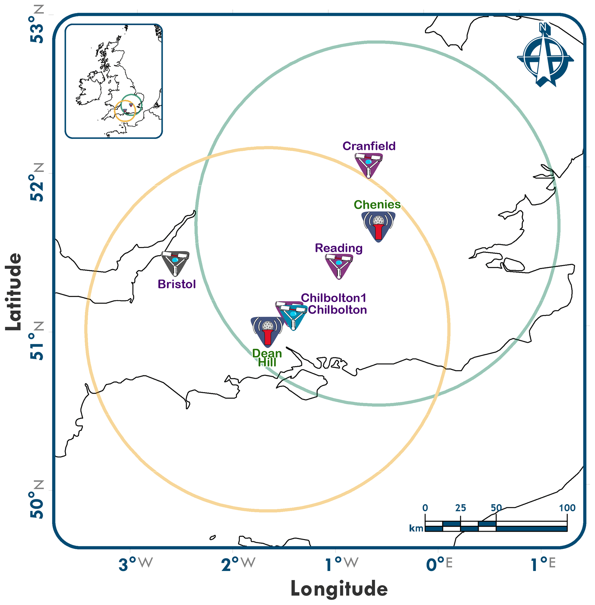
Figure 1Location of the radars (Chenies and Dean Hill) and disdrometers (Bristol, Chilbolton, Cranfield and Reading). The circles represent the coverage of each radar at a distance of 115 km (maximum coverage of the radars operating at short pulse lengths).
Table 1Polarimetric radar characteristics.

Note that PRF denotes pulse repetition frequency, RPM denotes revolutions per minute, SP denotes short pulse and LP denotes long pulse.
2.2 Disdrometer data sets
In this study, disdrometer data are used for verifying the consistency of the radar differential reflectivity measurements as the disdrometers are instruments that measure the drop size distribution (DSD) of precipitation. Several disdrometer data sets were collected from different projects with locations neighbouring the radar sites and matching time periods. These include disdrometers from the Chilbolton Facility for Atmospheric and Radio Research (CFARR), the Disdrometer Verification Network (DiVeN), and the University of Bristol (UoB) (see locations in Fig. 1 and Table 2).
CFARR operates a Joss–Waldvogel impact disdrometer (model RD-69) located at Chilbolton, Hampshire, southern England, that has provided continuous DSD data since 2003. The disdrometer converts the vertical momentum of a falling drop into signals whose amplitude depends on the diameter of the impacting drop. This device provides drop counts every 10 s over 127 bins ranging from 0.3 to 5 mm, with a sampling area of approximately 50 cm2 (Science and Technology Facilities Council et al., 2003). This instrument does not measure the fall velocity of precipitation particles, and therefore the device does not provide a hydrometeor classification. For this work, data were available from January to July 2018.
DiVeN was deployed in 2017, and the disdrometer network includes several Thies laser precipitation monitors in the UK that provide information on the quantity, intensity and type of precipitation (Pickering et al., 2019). The Thies disdrometer measures the diameters and fall velocities of the hydrometeors and categorises hydrometeors into different classes (drizzle, drizzle/rain, rain, ice, snow, wet ice, wet snow, graupel, wet graupel and hail). The disdrometer provides the number of drops recorded every minute over a matrix covering 20 diameter and 22 velocity classes. The diameters range from 0.125 to 8 mm; the velocities range from 0.0 to 20.0 m s−1, and the sampling area of the instrument is approximately 45.6 cm2 (Natural Environment Research Council et al., 2019). For this work, we selected three disdrometers operating near the radar sites, one at Chilbolton, Hampshire (herein Chilbolton1); one at Reading, Berkshire; and one at Cranfield, Bedfordshire, all located in England. Data were collected for precipitation events throughout 2018.
The UoB operates several Parsivel2 disdrometers, one of them located at Bristol, southwest England. This laser disdrometer measures the drop size distribution (DSD) and categorises the precipitation particles into several classes (drizzle, drizzle/rain, rain, rain/snow, snow, sleet, hail). The instrument provides the number of drops recorded every minute over a matrix covering 32 diameter and 32 velocity classes. The particle size includes 32 bins ranging from 0.2 to 25 mm, and the particle speed includes 32 bins ranging from 0.2 to 20 m s−1) (OTT HydroMet, 2016). The sampling area of this instrument is approximately 50 cm2. Data were collected for precipitation events throughout 2018.
Table 2Summary of radars (RAD) and disdrometers (DIS).
Note that D-CH denotes distance to the Chenies radar site and D-DH distance to the Dean Hill radar site.
Processing of disdrometer data
The raindrop size distribution (DSD) can be computed from the disdrometer data by (Ji et al., 2019)
where Di is the drop diameter (mm), ni is the number of drops counted during the sampling interval Δt (s) at the ith bin size, A (m2) is the sampling area of the disdrometer, Vi (m s−1) is the terminal velocity of the raindrops at the ith bin size and ΔDi (mm) is the ith bin width diameter interval. The sampling interval Δt was fixed to 60 s to ensure there are a sufficient number of measurements to compute a reliable DSD, which is also consistent with previous studies (Bringi et al., 2011; Ji et al., 2019). The terminal velocity of raindrops was computed by (Atlas et al., 1973)
where D is in millimetres and V is in m s−1. The disdrometers measure the DSDs with a 1 min sampling interval. The Thies and Parsivel disdrometers measure the terminal velocity of raindrops to classify precipitation particles based on the velocity–diameter relationships. Only those measurements classified as liquid rain were used in this analysis. The DSDs were fitted to a normalised gamma drop size distribution using the procedure given in Bringi et al. (2003), where the normalised gamma DSD is given by
Here f(μ) is given by
where Nw (m−3 mm−1) represents the normalised intercept parameter, Dm (mm) is the mass-weighted mean diameter and μ is the shape of the distribution. Dm is related to D0 (median volume diameter) for a gamma DSD by (Bringi et al., 2003)
From the above analysis, the parameters Nw, D0 (or Dm) and μ were retrieved for each 1 min measured DSD. Then Eq. (3) was used to compute the theoretical DSD, which was used as input to a T-matrix scattering model developed by Mishchenko (2000) and adapted to compute all the different polarimetric weather radar measurements, including ZH and ZDR, which are both used in this analysis. The scattering simulations were performed using the following assumptions: (i) the raindrop shape model from Thurai et al. (2007) (their Eq. (2) for D>1.5 mm, their Eq. (3) for mm, spherical raindrops otherwise); (ii) no canting angle distribution; (iii) maximum diameter for the integration fixed to 3D0; (iv) temperature of 10 ∘C, radar wavelength of 5.3 cm and elevation angle of 0∘.
3.1 Offset detection and monitoring of ZDR using vertical profiles (VPs)
The overall system bias (or offset) in ZDR can be estimated using VPs taken in light-rain events, as described in the literature review. The VPs represent averaged observations of the 360 vertical rays, reducing the variance in ZDR caused by the symmetry axis and the variety of shapes of the raindrops. Then the premise of this method is to use VPs related to light rain, where a deviation from 0 dB in the rain region of the VPs can be set as the ZDR offset. An in-depth discussion on the selection of this natural target to detect the ZDR offset is provided in Sect. 5.
The offset on ZDR can be detected and corrected by an automated operational procedure as follows.
-
It is necessary to detect the rain region on the VPs; this can be achieved by implementing the ML detection algorithm proposed by Sanchez-Rivas and Rico-Ramirez (2021) and then setting the ML bottom as a boundary. Values on the VPs below the bottom of the ML are likely related to precipitation in the liquid phase.
-
Once the rain region is identified on the VPs, thresholds related to light rain are set, and only VPs containing two or more consecutive bins of ZDR having corresponding values of 5 dBZ dBZ and ρHV>0.98 are kept for further calculations.
-
The ZDR offset is calculated for each VP related to light rain using the following expression:
where i represents a valid bin along the VP, n the number of valid bins below the melting layer and avoiding clutter echoes, the offset calculated from the vertical profile, and the bins of ZDR below the ML. Note that n includes bins from different azimuths. If is different from 0 dB, then ZDR needs to be calibrated.
-
Finally, ZDR PPI measurements at different elevation angles can be corrected by subtracting the offset computed in Eq. (6) to the original ZDR measurements using
where is the offset-corrected differential reflectivity, is the differential reflectivity measured by the radar and is the offset calculated from the vertical profiles.
3.2 Offset detection and monitoring of ZDR using quasi-vertical profiles (QVPs)
The QVPs of polarimetric variables provide insight into the evolution and structure of rain events through time, thus enabling monitoring the calibration of the radar variables. Hence, we propose a method to estimate the ZDR offset that can be applied to QVPs generated from lower-elevation scans with elevation angles of around 9∘ collected during light-rain events. The proposed method is based on the following rationale.
- a.
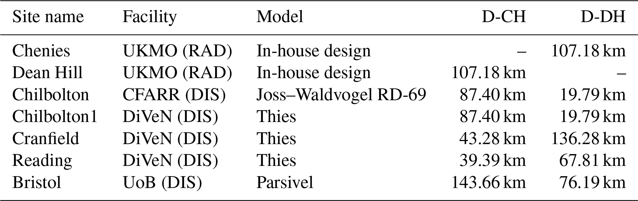
The rain region within the QVPs of ZDR is mostly uniform when the profiles are generated from data collected in light rain and near the radar as this region represents averaged observations of small oblate raindrops. Figure 2 portrays the radar coverage of two PPI scans at different elevation angles recorded by one of the radars. It can be seen that birdbath scans (and subsequent VPs) capture uniformly the rain region (between 1 and 2.5 km in height) developed above the radar (Fig. 2a). Similarly, the rain region below the bright band (located at 2.5 km in height) is mostly homogeneous for this particular PPI with an angle elevation of 9∘ (Fig. 2b).
- b.
The intrinsic value of ZDR for angles below 90∘ and collected in light rain is larger than zero, and it is elevation-dependent, as demonstrated by Bringi and Chandrasekar (2001) and formulated by Ryzhkov et al. (2005a) as
where Zdr(0) and Zdr(θ) represent the differential reflectivity at a linear scale at elevation angles of 0∘ and θ∘, respectively. Figure 3 displays the theoretical variation in ZDR with elevation angle. It can be seen that the difference in ZDR values between an elevation below 10∘ and the elevation of 0∘ is negligible. In fact using Eq. (8) for results in Zdr values very close to each other; that is
Hence, ZDR radar measurements collected at elevation angles below 10∘ are similar to those collected at lower elevation angles, and so they do not add additional uncertainty to the offset correction method. However, Fig. 3 also shows that ZDR values for lower elevation angles have a wide range of values (e.g. between 0 and 2 dB in this figure) compared with elevation angles of 90∘ in which ZDR values close to zero are expected. This represents a challenge for our approach, and therefore we have to constrain the Zdr measurements used to compute the offset into a narrow band as explained next.
- c.
We simulated a wide range of DSDs using the range of parameters described in Bringi and Chandrasekar (2001) expected in real storm events using the following parameter ranges:
We randomly generated 10 000 sets of DSD parameters (Nw, D0 and μ) uniformly distributed within the ranges defined above. Then we use Eq. (3) to simulate the DSDs, which are used as input to a T-matrix scattering model to compute ZH and ZDR. The scattering simulations are performed using the same assumptions described in the section “Processing of disdrometer data”. The results of these simulation are shown in Fig. 4a, which depicts the theoretical variation in ZDR versus ZH, which is consistent with previous studies (Bechini et al., 2008; Bringi et al., 2006; Giangrande and Ryzhkov, 2005; Ryzhkov et al., 2005a). Figure 4a shows that ZDR increases with ZH and also that ZDR has a wide range of values for a given value of ZH. However, the expected range of ZDR measurements in light rain (e.g. for ZH<20 dBZ) becomes narrow and gives ZDR<0.6 dB (see zoomed-in region in Fig. 4a).
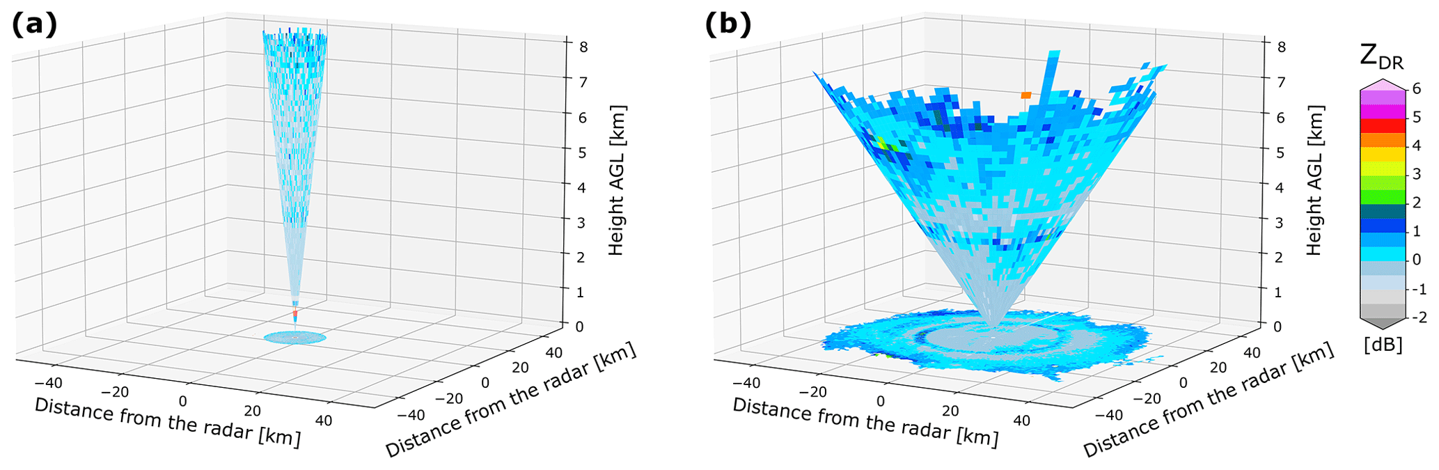
Figure 2Representation of the radar conical coverage using (a) a birdbath scan, useful for building VPs, and (b) a 9∘ PPI scan, used to generate QVPs.
Based on the premises described above, we propose an operational method to compute and correct the ZDR offset using QVPs as described below.
-
As in the VP method, the rain region is identified in the QVPs using a ML detection algorithm to set the ML bottom as a boundary. Values below this height are likely related to precipitation in the liquid phase. Additionally, a maximum height limit of 3 km is set to this ML bottom boundary to reduce the range effects inherent to the generation process of the QVPs. The maximum height limit of 3 km seems to work well in the UK, but it might need to be adjusted in other regions.
-
Using the theoretical variation in ZH and ZDR given in Fig. 4a, we compute the mean dependencies but limited to a narrow range related to light rain ( dBZ), as shown in the zoomed-in box in Fig. 4a. This yields a mean value of dB, which is set as the intrinsic value of ZDR in light rain at ground level for lower-elevation scans. This value is compared to ZH−ZDR values computed from disdrometer measurements (see Fig. 4b), confirming the good agreement between theoretical and measured ZDR values.
-
Various thresholds are set to detect QVPs related to light rain and discard bins within the QVPs related to mixed-phase precipitation. Thus, only QVPs containing three or more consecutive bins of ZDR with corresponding values of 0 dBZ dBZ and ρHV>0.985 on the QVPs of ZH and ρHV, respectively, are kept for further calculations. Note that the threshold set for ZH is the same as the range selected in the DSD simulations, whereas the threshold set for ρHV is more strict than in the method based on VPs in order to discard bins within the QVPs not related to light rain.
-
The average value of ZDR is computed, calculating one value per QVP related to light rain:
-
Finally, ZDR measurements can be corrected by
where is the offset-corrected differential reflectivity, is the differential reflectivity measured by the radar and is the offset calculated from the QVPs.
Figure 3Theoretical dependencies of ZDR at different elevation angles. Highlighted area shows the small variation in ZDR for elevation angles below 10∘.

Figure 4(a) Simulated ZH−ZDR dependencies expected in real storm events; (b) ZH−ZDR dependencies measured by several types of disdrometers at different locations.
We processed the radar data sets collected by two operational weather radars throughout 1 year of precipitation events to generate VPs and QVPs of polarimetric variables as described in Sect. 2.1. Then we applied both ZDR offset-correction methods to the generated VPs and QVPs to compare the results of the ZDR calibration.
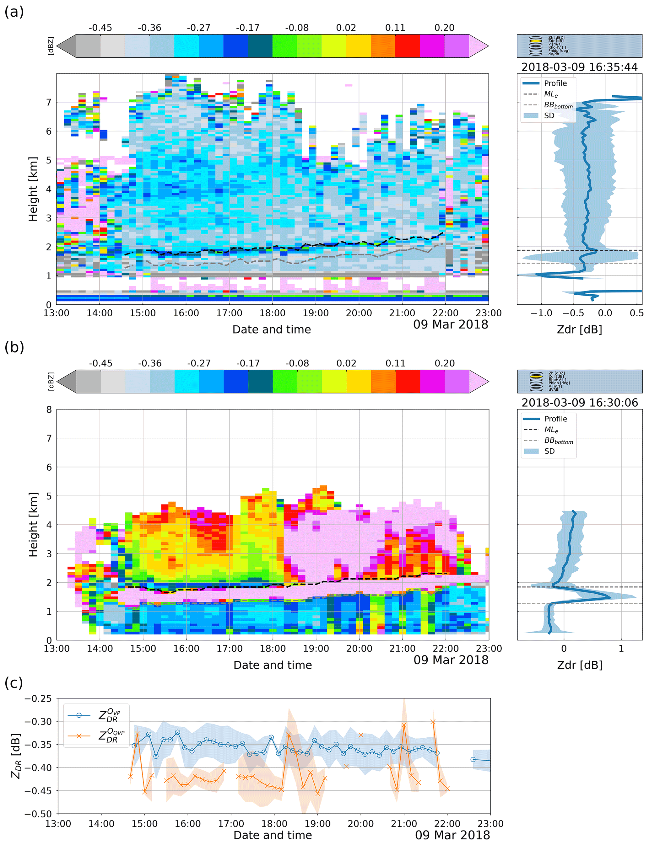
Figure 5Rain event recorded by the UKMO Chenies radar on 9 May 2018. Panel (a) shows a collection of ZDR VPs in a height-versus-time plot along with the melting level (MLe) and the bottom of the melting layer (BBbottom). Its right panel depicts a single VP and its standard deviation (SD). Panel (b) shows the same as in (a) but using QVPs of ZDR. Panel (c) shows the ZDR offset computed using VPs (blue line, circle markers) and QVPs (orange line, cross markers); the filled areas represent the computed standard deviation for each data point.
We present a rain event recorded in southern England by the Chenies radar to exemplify the above-mentioned processes. In Fig. 5a, the left panel shows VPs (each one representing the mean value of 360 rays) of ZDR in a height-versus-time (HTI) plot related to a rain event. In contrast, the right panel shows a single VP taken from the same event. Note that the first kilometre of the VPs is contaminated with spurious echoes; hence all bins below this height were discarded from the analysis. The HTI plot shows that the values of ZDR deviate from 0 dB in the rain medium, i.e. below the bottom of the bright band (BBbottom); thus ZDR needs to be calibrated. The single VP plot enables an in-depth analysis of the profile characteristics. For example, it can be seen that ZDR values within the rain region (below 1.5 km in height) are close to −0.35 dB and also that its standard deviation (SD) remains relatively steady. But this changes in the ML, where the VP turns noisy and produces a higher standard deviation. However, dry aggregated snow signatures are visible above 2 km in height (at the top of the melting layer), where the ZDR values are similar to those observed for liquid precipitation (∼0.37 dB), confirming the reliability of dry snow in detecting the ZDR offset. These characteristics are consistent throughout the entire event.
On the other hand, Fig. 5b shows QVPs of ZDR values generated from data related to the event described above. It can be seen that there are clear signatures of the melting layer within the QVPs that are useful to classify the hydrometeors' phase. The single QVP plot shows that the standard deviation of the averaged values used to generate the QVP is smaller in the rain region (below 1.35 km) compared to the standard deviation observed within and above the ML. Moreover, the signatures of dry snow are not clearly visible, and the values observed for rain particles differ from those seen at the top of the ML, thus hampering using dry snow as the calibration target for our data sets. After applying the proposed method, the averaged value of ZDR in the rain region is −0.26 dB, which, along with the computed intrinsic value of ZDR (0.18 dB), results in an offset of −0.44 dB, which is close to the offset calculated using the VP method (−0.35 dB).
Figure 5c shows the temporal variation in the ZDR offset for both VP and QVP methods. For this precipitation event, the differences between methods are around 0.1 dB. Still, it is worth mentioning that exhibits values that remain relatively constant during this event, whereas the values of show greater variation and are not altogether far from . It is also important for this event that the number of valid VPs is larger than the number of QVPs classified as valid according to the proposed constraints described in the method. A discussion on the selection of the natural targets to detect the ZDR offset and the performance of the proposed method is provided in Sect. 5.
4.1 Validation of the QVP-based approach using birdbath scans
The QVP-based approach will be assessed by comparing its results with the “true offset” computed from the VP-based method since it is widely accepted and has been proven effective, as described in the literature review. Therefore, it is essential to highlight that the errors in the ZDR calibration based on QVPs are relative to the traditional method. Additionally, both methods will be compared to independent measurements provided by the disdrometers.
Figure 6 shows the temporal variation in the ZDR offset for the two radar data sets used in this work. For the Chenies radar data set (Fig. 6a), it can be seen that the offset in ZDR computed using the birdbath method fluctuates between −0.2 and −0.7 dB during most of the year. During February 2018, filters were installed at the Chenies radar, introducing a variation into the radar calibration that can be observed at this period (Timothy Darlington, Met Office, personal communication, 2021). The proposed method based on QVPs proves to be effective as the ZDR offset values are similar to those calculated using VPs. For the Dean Hill radar data sets, the ZDR offset varies in a broader range, but as above, the computed offset is similar in both methods. Similarly, an upgrade implemented on the Dean Hill radar during October 2018 modified the ZDR calibration (Timothy Darlington, Met Office, personal communication, 2021), changing from −0.2 to 0.5 dB at around this time of the year. However, a few points throughout the entire year exhibit more significant differences. This shows that some profiles may surpass the constraints set to reject QVPs that do not meet the light-rain criteria. Averaging the entire radar domain plays a key role here, as mixed-phase precipitation can affect the QVPs (see Discussion in Sect. 5). Additionally, Fig. 6 shows two particular rain events (zoomed-in boxes in this figure) for a deeper visualisation of the calibration methods, where it can be seen that both methods produce similar results.
Figure 6 also shows that the number of profiles detected by each method is different. The VP-based method detects a larger number of profiles that meet the criteria of light rain, especially for the Dean Hill radar data set. For this radar data set, the number of valid profiles detected by the QVP-based approach represents 47 % of the profiles detected by the VP-based method. This difference is not that big for the Chenies radar data set, as the number of profiles detected by the QVP-based method represents the 78 % of profiles detected by the VP-based method. Although this is a limitation of the method, this ensures that only those QVPs due to light rain and with high ρHV values are used for the estimation of the ZDR offset. In this case, we use the last valid QVP-based ZDR offset, which is then compared to the ZDR offset computed by the VP-based method.
Finally, we observed an overall relative error in the ZDR offset using QVPs of ±0.1 dB compared to the method based on VPs. This increases the confidence in using the proposed method based on QVPs.
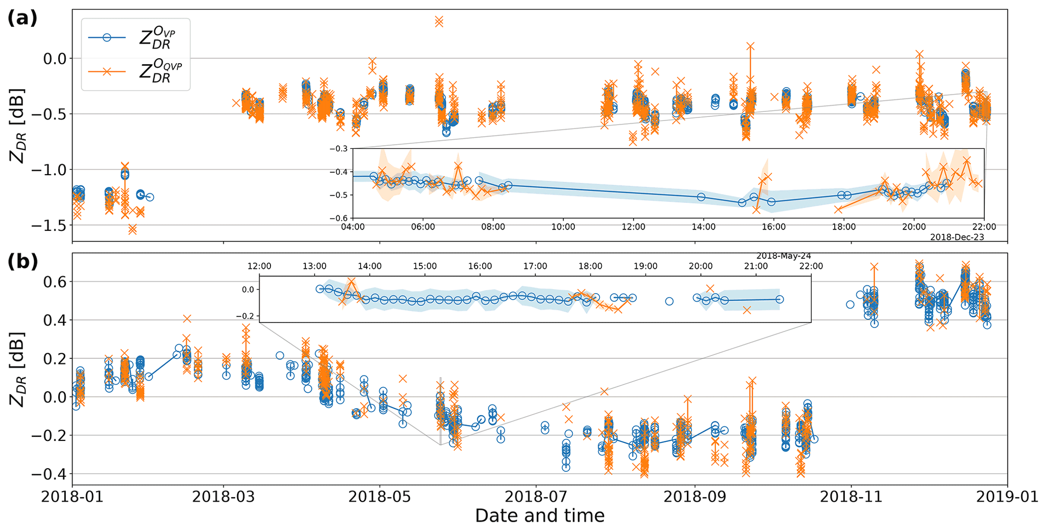
Figure 6Temporal variation in the ZDR offset on two weather radars during 1 year of rain events. The top panel shows the variation on the Chenies radar site, whilst the bottom panel depicts the offset variation at the Dean Hill radar site. The case of a rain event on 9 March 2018 is zoomed in on in both panels for an in-depth examination. The date is indicated in the format year-month.
We evaluate the outputs of each method for the two different radar sites using metrics like the correlation coefficient (r), the mean absolute error (MAE) and the root mean squared error (RMSE). To effectively assess the performance of the QVP-based approach and its temporal variation, each computed offset value is stored as the radar ZDR offset until a new one is detected; e.g. in Fig. 6b, for the case on 24 May 2018, the VP-based method yields a constant offset value of around −0.15 dB between 13:05 and 18:05 Greenwich mean time (GMT – this time zone applies throughout), whereas the QVP-based method only detected a handful of valid QVPs for the same time period. However, the offset is similar at those points in time, with differences of around ±0.1 dB. It is worth mentioning that this is a warm-rain event, and only a few QVPs meet the criteria set for detecting light rain.
Figure 7 shows a comparison of the ZDR offset estimated by both methods for both radars for the entire year. The results show that the ZDR offset for the Chenies radar was between −0.7 and −0.1 dB, with a small number of events showing an offset of around −1.3 dB. For the Dean Hill radar, the ZDR offset was between −0.4 and 0.6 dB. The figure shows a good correlation between the outputs of both methods, where the relative performance of the QVP-based method is in good agreement (±0.1 dB) with the true offset computed from birdbath scans (VP-based method).
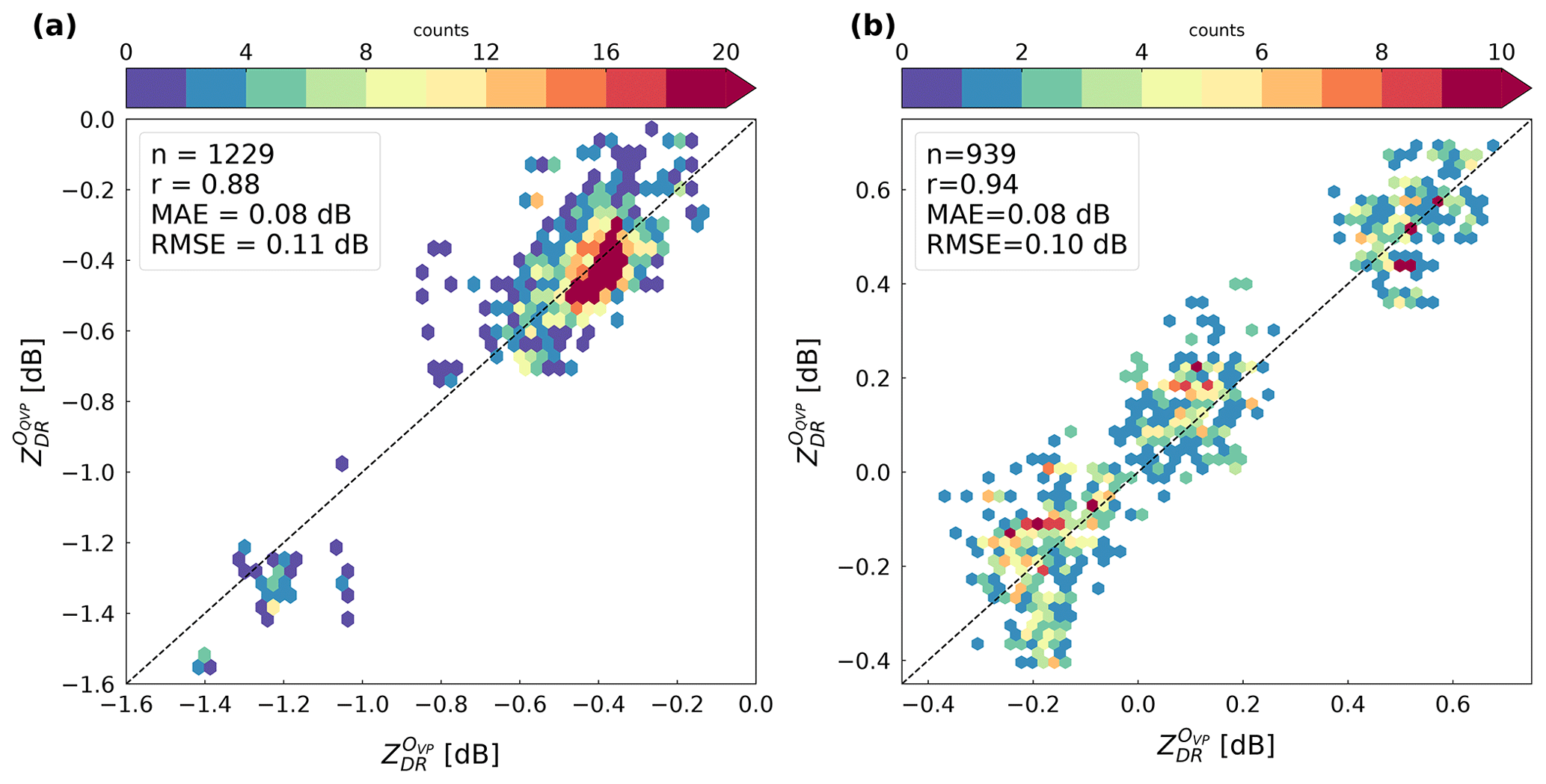
Figure 7Comparison of ZDR offsets computed with QVPs and VPs. The scatter density plot shown in (a) provides metrics for evaluating the methods applied to the Chenies radar data set, whereas (b) shows the same as in (a) but for the Dean Hill radar data set.
4.2 Differential reflectivity comparison using radar and disdrometers
Several validation procedures of the proposed method for correcting the ZDR offset were performed utilising the disdrometer data sets described in Sect. 2.2. The fitted normalised gamma DSDs allows the estimation of the reflectivity and the differential reflectivity at ground level, enabling the validation of the QVP-based method.
First, we compare the radar-calibrated ZDR measurements by the two approaches described in the previous sections at the disdrometer locations. Only individual radar bins exactly over the corresponding disdrometers locations are considered for comparison. Based on the distance between the radars and the disdrometers, we link the Cranfield and Reading disdrometers to the Chenies radar, whereas the Chilbolton1 disdrometer will be compared to the Dean Hill radar. The disdrometer located at Bristol was not used in this analysis because it is too far from both radar sites. In addition, we use the hydrometeor classification produced by the Thies disdrometers to evaluate the radar measurements related to liquid precipitation, as these disdrometers provide information about the rain type and intensity. This classification is helpful to discard DSDs related to snow or hail.
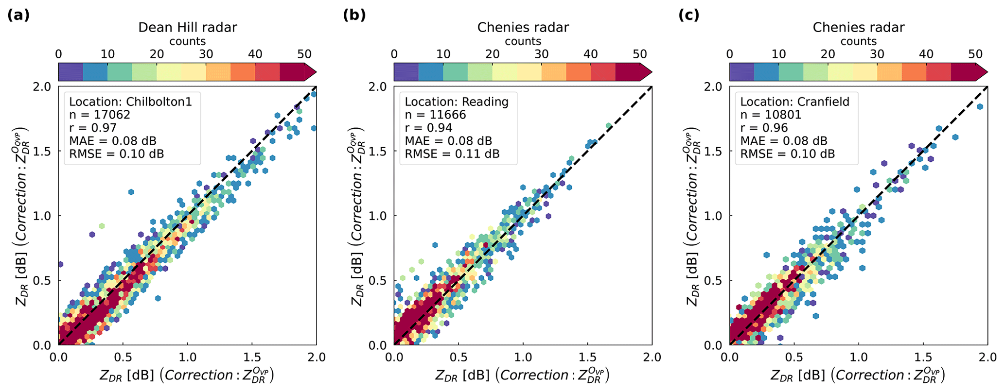
Figure 8Scatterplots between calibrated ZDR measurements using VPs and QVPs. Each plot represents radar ZDR measurements at different locations and filtered using precipitation and intensity classifiers gathered from disdrometers.
Figure 8 shows the scatterplots using both methods to calibrate ZDR measurements at disdrometer locations. For the Chenies radar data, we applied Eqs. (7) and (11) to correct the ZDR offset in PPI scans taken at a 0.5∘ elevation angle, whilst for the Dean Hill data, we applied the same equations to correct the ZDR offset but on PPI scans taken at a 2∘ elevation angle as lower elevations are beam-blocked or contaminated with ground clutter. The proposed approach based on QVPs proves effective as an accuracy of ∼0.1 dB is achieved in all analysed cases when comparing the ZDR measurements calibrated using QVPs against ZDR measurements calibrated using the traditional method based on VPs.
In addition, we compare the polarimetric variables measured by the radar with the variables derived from disdrometer DSDs. We discard data not related to liquid precipitation by using the classifiers available on the disdrometer data sets and using only radar data with corresponding values of ρHV≥0.98. As described in Sect. 2.1, algorithms for removing non-meteorological echoes and for correcting the signal attenuation are applied to radar data sets when appropriate. Regarding the disdrometer data sets, we applied a moving-average filter (window size of 5) to reduce data fluctuations due to the finer time resolution of the disdrometer data (1 min) compared to the radar data sets (5 min). Furthermore, to include data collected by the CFARR Chilbolton disdrometer (model Joss–Waldvogel, not capable of classifying the rain type), we used the classification from the Thies disdrometer (Chilbolton1) to discard data from the former not related to rain, as these two disdrometers are close to each other (just a few metres apart).
Figure 9 shows the comparison between calibrated ZDR radar measurements and ZDR derived from disdrometer observations collected throughout 1 year of precipitation events. The ZDR measurements shown in Fig. 9a were calibrated with VPs, whereas the ZDR measurements shown in Fig. 9b were calibrated with QVPs. The results show comparable errors using either of the ZDR calibration methods, confirming the good performance of the proposed method (the MAE and RMSE are below 0.3 dB and 0.4, respectively, in all disdrometer sites for both calibration methods). Although these errors are more significant than the errors shown in Fig. 8, these are also due to additional factors such as sampling errors (e.g. comparing point disdrometer observations with areal radar measurements), variations in ZDR measurements aloft (e.g. comparing radar observations aloft with ground disdrometer observations), timing errors (e.g. disdrometer measurements are integrated over time each minute, whereas radar observations are taken in a few seconds every 5 min) and uncertainty in the estimation of ZDR from DSD measurements. As mentioned above, scans taken at different elevation angles are used on each radar to capture the precipitation occurring above the disdrometer, adding some uncertainty to the interpretation of these results.

Figure 9Scatterplots between radar and disdrometer ZDR measurements at several locations: panel (a) shows scatter density plots of ZDR offset-corrected using VPs at two different radar sites versus ZDR derived from disdrometer data; panel (b) shows the same as in (a), but the radar ZDR measurements are calibrated applying the QVP-based method.
4.2.1 Case study – 24 May 2018
Figure 10 portrays a rain event recorded by the Dean Hill radar at an elevation angle of 2∘ and data from two disdrometers located at the same location (Chilbolton Observatory). The top panel shows a good agreement between the radar reflectivity and the reflectivity derived from disdrometer DSDs as there is a similar trend in all data sets. Overall, the correlation of ZH for the whole year of data between the radar data set and the two disdrometers is ≥0.80 (graph not shown). On the other hand, the bottom panel of Fig. 10 illustrates the calibrated ZDR measurements by both methods and the ZDR measurements derived from disdrometer observations. It can be seen that the ZDR measurements calibrated with the proposed QVP-based method are in good agreement with the ZDR measurements calibrated with scans collected at vertical incidence as a maximum difference of ±0.1 dB is observed. Both methods are consistent with the data derived from the two disdrometers located at the Chilbolton Observatory.
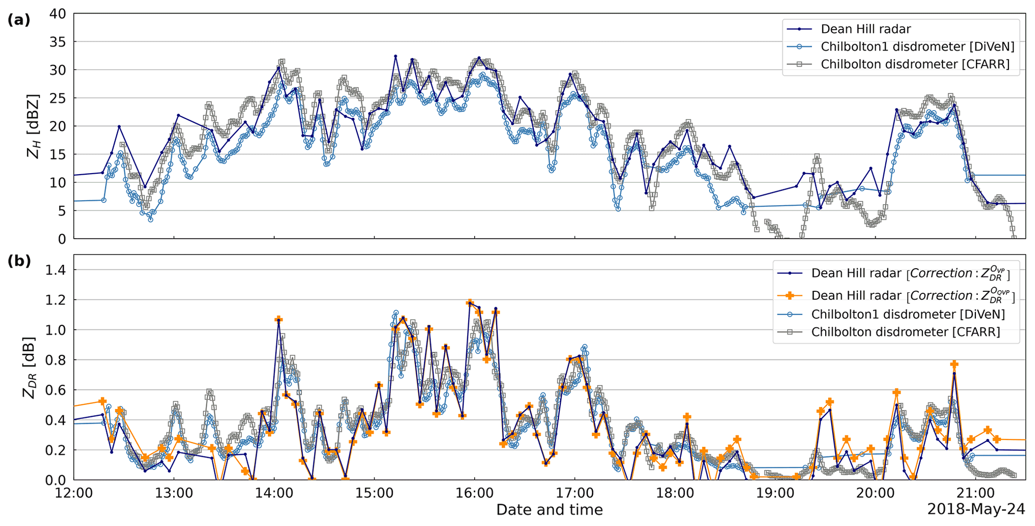
Figure 10Time series of disdrometer and radar data related to a precipitation event registered in southern England: (a) reflectivity (ZH) simulated from disdrometer DSD data at two nearby locations and ZH measured by the C-band Dean Hill weather radar at an angle elevation of 2∘; (b) differential reflectivity (ZDR) measured by the Dean Hill radar and offset-corrected using two different approaches and ZDR simulated from two disdrometers.
4.2.2 Case study – 14 October 2018
Figure 11 shows data collected by the Chenies radar at an elevation angle of 0.5∘ and data from two disdrometers (Cranfield and Reading) located at different locations. As above, ZH values are similar on the three devices. Figure 11a shows that the radar tends to underestimate the reflectivity, with differences of the order of 5–10 dBZ between the radar data and the Cranfield disdrometer, especially at times between 05:30 and 08:00. For this site, the correlation of ZH for the whole year of data between the radar data set and the disdrometers is acceptable (r≈0.7) considering the distance between devices (graph not shown). Consequently, the ZDR measured by the radar is in general smaller compared to the ZDR derived from the Cranfield disdrometer (see Fig. 11b). However, it is important that both ZDR calibration methods yield similar trends in both VP- and QVP-based methods, where maximum differences of 0.2 dB are observed for a short period of time, between 08:30 and 08:45.
On the other hand, Fig. 11c and d show data measured by the Chenies radar and the Reading disdrometer. It can be seen that there is an excellent agreement between devices for both ZH and ZDR. It is important that ZDR values corrected using the proposed method based on QVPs exhibit almost the same pattern compared to the ZDR values corrected using the VP-based method.
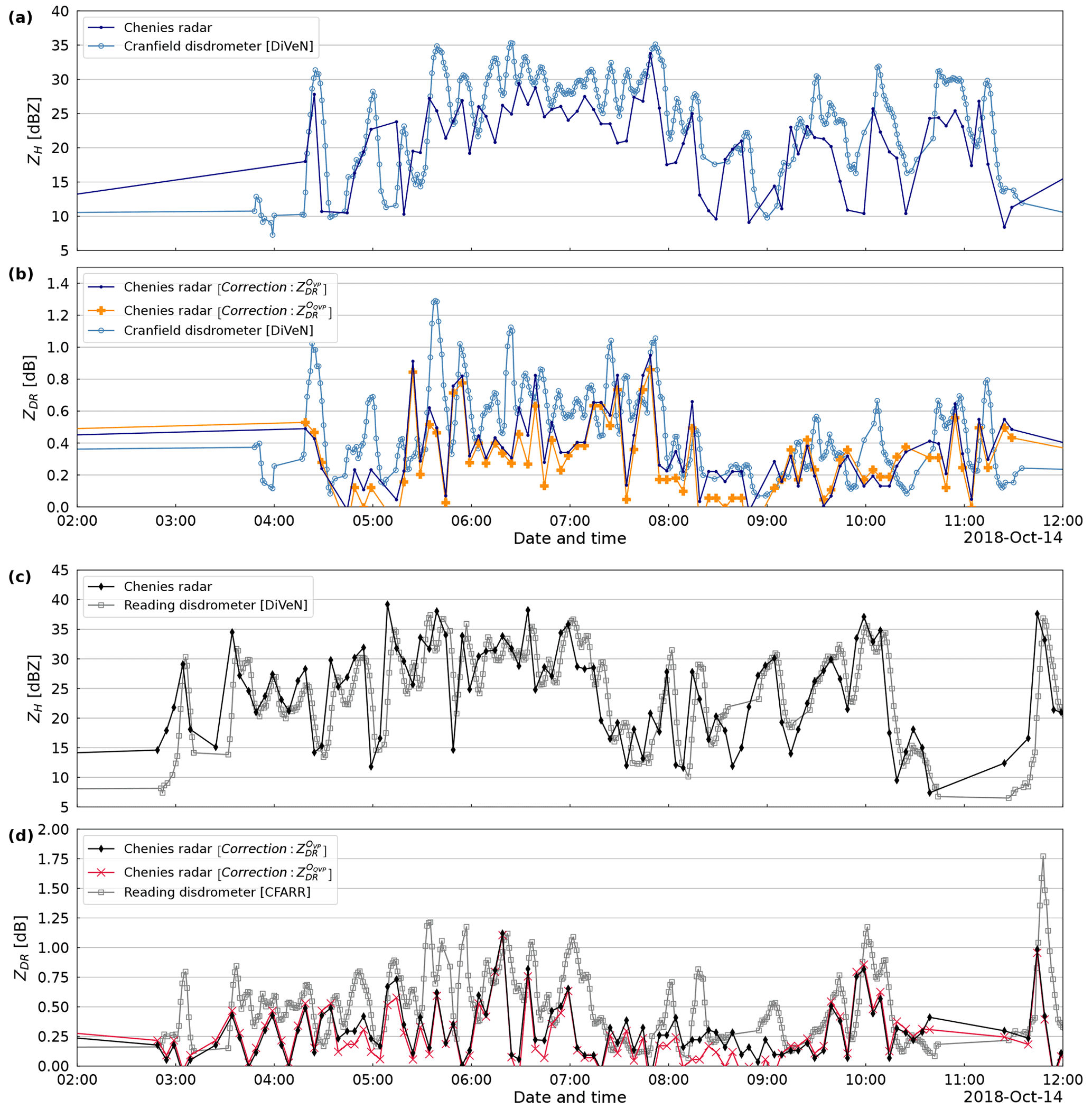
Figure 11Time series of disdrometer and radar measurements. Panels (a) and (c) show the reflectivity, whereas panels (b) and (d) show the differential reflectivity.
This work reviews the use of QVPs of polarimetric radar measurements to estimate and monitor the overall system bias (or offset) in the differential reflectivity. Although several sources of error affect this variable, we focused on detecting and correcting the overall system bias. It is important to calibrate ZDR measurements as this variable is a crucial input to hydrometeor classification methods (Al-Sakka et al., 2013; Park et al., 2009), attenuation correction schemes (Bringi et al., 2011; Gou et al., 2019) or QPE algorithms (Chandrasekar and Bringi, 1988; Cifelli et al., 2011; Giangrande and Ryzhkov, 2008; Ryzhkov et al., 2005b; Vulpiani et al., 2009). Ryzhkov et al. (2005a) demonstrated that keeping the bias below ±0.2 dB generates accurate and reliable radar products.
Previous works have developed methods to compute the ZDR offset using different targets, like light rain (Bechini et al., 2008; Gorgucci et al., 1999), dry snow (Ferrone and Berne, 2021; Ryzhkov et al., 2005a), ice (Bringi et al., 2006), sun spikes (Chu et al., 2019; Holleman et al., 2010) or turbulent eddies (Richardson et al., 2017). Most of these methods are based on measurements taken at high elevation angles that reduce the intrinsic variability in ZDR. However, mechanical restrictions may prevent some radars from scanning at such high elevation angles; therefore, we evaluate a new approach to compute and correct the offset in radar ZDR measurements based on QVPs of polarimetric variables built from PPI scans taken at lower elevation angles of around 9∘. The proposed method is an alternative method to calibrate ZDR measurements, but the traditional method based on VPs should be used instead if these vertical scans are available. As described in Sect. 3.2, we set light rain as the target to compute the ZDR offset, using QVPs mainly to reduce the variability in ZDR. Regarding the selection of this natural target, it is worth saying that we also explored the use of dry snow to derive the ZDR offset. Dry aggregated snow can be found 1 or 2 km above the melting layer in stratiform clouds (Brandes and Ikeda, 2004; Ryzhkov et al., 2005a). Ryzhkov et al. (2005a) explored high-elevation-angle scans (∼ 40–60∘) and observed that dry aggregated snow yields distinctive polarimetric signatures, i.e. values of ZDR close to 0 dB, demonstrating that this target can be used to detect the ZDR offset. Consequently, we analysed hundreds of polarimetric profiles (both VPs and QVPs data sets) and found that such a signature of dry snow is only observable on the VPs in our data set. This effect can be seen in Fig. 5a, where similar values of ZDR can be seen on both light rain (below the melting layer bottom) and dry snow (above the melting layer top). Conversely, in the QVP data set (obtained at lower elevation angles of 9∘), we observed that values of ZDR in the rain medium were not consistent with those observed aloft, as shown in Fig. 5b. This lack of clear signatures of dry snow on QVPs is probably related to the beam broadening and non-uniform beam-filling effects, expected when the QVPs intercept the ML and regions above 9∘ elevations. As shown in the right panel of Fig. 5b, the standard deviation (blue area) increases within and above the ML due to the presence of mixed-phase particles, hence complicating the estimation of the ZDR offset using such meteorological targets. This is the reason why we could not use QVPs built from relatively low elevation angle scans (<10∘) and set dry snow as the target to derive the ZDR offset.
But using QVPs in light-rain events for detecting the ZDR offset also presents several risks. First, it is important that there is an inherent variability in ZDR in light rain. This is shown in Fig. 4a, where it can be seen that the variability in ZDR increases with larger values of ZH. Thus, we propose a constraint to reduce the variability in ZDR; i.e. . This range is a compromise to avoid having significant variations on ZDR but still keep enough QVPs related to light rain in the analysis and enable the reliable detection of the ZDR offset. In addition, the inherent averaging process in the QVP construction may wash out some key microphysical processes within the precipitation events. Thus, we proposed several constraints to minimise these effects. For example, we imposed a limit of 3 km in height within the QVPs to apply our method: as shown in Fig. 2b, the coverage of the PPI scans at a 9∘ elevation angle captures a mostly uniform volume in the rain region (below 2.5 km). For this elevation angle and a height of 3 km, the base diameter of the cone is around 37 km. Hence we consider that the azimuthal averaging procedure to generate the QVPs below this height reduces deviations in ZDR and enables proper monitoring of the calibration of this variable. Additionally, we define thresholds to discard values within QVPs not related to light rain; e.g. Fig. 5b shows a collection of QVPs related to a rain event. Most of the QVPs show a constant value of ZDR below the ML, whilst outlier values can be discarded by checking their corresponding values on the QVPs of ZH and ρHV (plots not shown). This figure also shows that the values of ZDR above the rain region are loosely correlated to the ZDR offset, hence hampering the use of meteorological targets like snow or ice. It is clear that dry snow has lower natural ZDR variability compared to light rain when using high tilts (40–60∘). However, this variability increases at lower elevations, and the QVPs are affected by this issue. This is why we restricted the height within the QVPs along with thresholds in ρHV in an effort to keep the variability at a minimum.
It is worth mentioning that setting the boundaries of the melting layer correctly within the QVPs is a critical step towards detecting reliable values of the ZDR offset, as this enables the identification of echoes related to liquid precipitation. Allabakash et al. (2019), Griffin et al. (2020), Lukach et al. (2021) and Sanchez-Rivas and Rico-Ramirez (2021) demonstrated that heights of the ML top and bottom could be accurately estimated using QVPs. We consider that QVPs without ML signatures are filtered by this requirement, thus reducing the uncertainty of using QVPs of polarimetric variables that do not depict light stratiform rain.
To validate the proposed approach, we implemented an operational procedure to detect the ZDR offset using light-rain measurements taken at vertical incidence. This method was proposed initially by Gorgucci et al. (1999), and it is a boilerplate practice that has been tested on several radar campaigns and has confirmed its reliability by keeping the ZDR offset below 0.2 dB (Bechini et al., 2002; Frech and Hubbert, 2020; Gourley et al., 2009; Louf et al., 2019). Figures 6 and 7 show the good agreement between both methods: the proposed method based on QVPs shows maximum differences of 0.1 dB compared to the method based on VPs. A few data points exhibit larger variation, but this is mainly caused by vague polarimetric signatures of the ML (no peaks within the polarimetric profiles, especially on those generated from ρHV measurements), misleading the ML detection algorithm and, thus, the classification of the particles in the liquid phase. The good performance of the method based on QVPs is also confirmed in Fig. 8, where we evaluated data classified by the disdrometers as related to light to moderate rain rates, and the differences between both ZDR calibration methods remain around 0.1 dB.
Figures 9–11 show a comparison between radar and disdrometer data. It is important to keep in mind that there is some uncertainty in the interpretation of these results, such as (i) the spatial distribution of radar measurements and the well-known discrepancy when comparing it to a fixed-point location, (ii) the impact of the signal attenuation in ZH and ZDR, (iii) the distance between the radars and the disdrometers, (iv) the use of PPI scans collected at higher elevation containing issues related to beam blockage or clutter contamination, and (v) the different temporal resolution of each device. However, the errors (MAE and RMSE) between ZDR measured by the radar and ZDR derived from disdrometers are below 0.4 dB in all cases, which is acceptable considering the factors mentioned above but also that this analysis includes 1 year of data related to precipitation events. Furthermore, we compared the disdrometer-derived ZDR measurements with radar ZDR measurements but without applying the offset correction procedure, and we observed bigger discrepancies between data sets, reaching differences of the order of 1 dB (plots not shown).
Finally, the case studies shown in Figs. 10 and 11 confirm the good performance of the proposed method to correct the ZDR offset. These events, related to moderate to intense rain events, exhibit differences below ±0.2 dB. These results are in good agreement with the required accuracy established by Ryzhkov et al. (2005a) to generate reliable quantitative precipitation estimates using polarimetric weather radar data.
In this work, we have evaluated different methods for monitoring the calibration of the radar differential reflectivity (ZDR). We explored the use of vertical profiles to calibrate the radar differential reflectivity. Light rain or dry snow are excellent targets to detect the ZDR offset, and we consider that these methods must be used when possible. However, some radar systems cannot perform scans at such high elevation angles. Thus, we proposed a novel, operational method to calibrate ZDR using QVPs of polarimetric variables built from low-elevation scans. This method has the main advantage of not depending on scans taken at vertical incidence or high elevation angles. However, it relies on detecting QVPs depicting stratiform light-rain events (common in the UK), but it may not be suitable for places where heavy-rain events are recurrent. Moreover, we are not suggesting that our approach should replace the well-known ZDR calibration method based on birdbath scans.
In addition, we carried out several trials using other meteorological targets like dry snow, but the results were inconclusive. Targeting areas above the melting layer exacerbate the beam broadening and non-uniform beam-filling problems as the range increases. These circumstances complicate using dry snow or other solid-phase targets to detect the ZDR offset on QVPs built from relatively low elevation scans. Thus, we selected the use of light rain, but we proposed several constraints to minimise the variability in ZDR in this media. Future work may implement a previous hydrometeor classification on the QVPs to improve this method. The proposed method is based on a reference ZDR value expected at ground level derived from a wide range of DSDs using a range of parameters expected in real storm events. This value (0.18 dB) was computed using constraints related to light rain using ZH. Additionally, we compared this theoretical ZDR value to real data derived from disdrometer observations, observing consistency between data.
We applied both methods to precipitation events collected by two C-band weather radars for the whole year of 2018. The proposed method to detect the offset in ZDR using QVPs was compared against the true offset computed from VPs. We observed a good agreement between both methods, as the MAE and the RMSE are within ±0.1 dB. However, we are aware that this is a relative evaluation; thus, we also implemented evaluation methods using disdrometer measurements. We compared radar ZDR measurements with ZDR measurements derived from disdrometer observations, obtaining a good agreement between the various data sets. This long-term evaluation of our method includes different types of precipitation events, ranging from light to heavy rain. We consider that this evaluation process demonstrates the efficacy of the proposed constraints to filter unsuitable QVPs. The proposed method using QVPs generated from PPIs proved to be effective for calibrating and monitoring the radar differential reflectivity as our results are close to those produced by the traditional method that uses birdbath scans.
Disdrometer data collected by the Chilbolton Facility for Atmospheric and Radio Research (CFARR) are available at https://catalogue.ceda.ac.uk/uuid/aac5f8246987ea43a68e3396b530d23e (Science and Technology Facilities Council et al., 2003); Chenies C-band rain radar dual-polarisation products are available at https://catalogue.ceda.ac.uk/uuid/bb3c55e36b4a4dc8866f0a06be3d475b (Met Office, 2013); Dean Hill C-band rain radar dual-polarisation products are available at https://catalogue.ceda.ac.uk/uuid/5b22789f362c43f3b3d1c65bc30c30ee (Met Office, 2021); DiVeN particle diameter and fall velocity measurements are available at http://catalogue.ceda.ac.uk/uuid/001b9640fdb1453aa95a222ba423580e (Natural Environment Research Council et al., 2019); disdrometer data collected at the UoB are available from the authors upon request.
DSR was responsible for carrying out the experiments, data analysis and writing of the paper. MARR provided supervision of the work and contributed to the writing of the paper.
The contact author has declared that neither they nor their co-author has any competing interests.
Publisher’s note: Copernicus Publications remains neutral with regard to jurisdictional claims in published maps and institutional affiliations.
This work was carried out using the computational facilities of the Advanced Computing Research Centre, University of Bristol (http://www.bris.ac.uk/acrc/, last access: 5 November 2021). We thank the two anonymous reviewers for their constructive comments.
This research has been supported by the Consejo Nacional de Ciencia y Tecnología (CONACYT (grant no. 637289)) and the Engineering and Physical Sciences Research Council (EPSRC (grant no. EP/I012222/1)).
This paper was edited by Gianfranco Vulpiani and reviewed by two anonymous referees.
Allabakash, S., Lim, S., and Jang, B. J.: Melting layer detection and characterization based on range height indicator-quasi vertical profiles, Remote Sensing, 11, 23, https://doi.org/10.3390/rs11232848, 2019. a
Al-Sakka, H., Boumahmoud, A. A., Fradon, B., Frasier, S. J., and Tabary, P.: A new fuzzy logic hydrometeor classification scheme applied to the french X-, C-, and S-band polarimetric radars, J. Appl. Meteorol., 52, 2328–2344, https://doi.org/10.1175/JAMC-D-12-0236.1, 2013. a, b
Atlas, D., Srivastava, R. C., and Sekhon, R. S.: Doppler radar characteristics of precipitation at vertical incidence, Rev. Geophys., 11, 1–35, https://doi.org/10.1029/RG011i001p00001, 1973. a
Bechini, R., Gorgucci, E., Scarchilli, G., and Dietrich, S.: The operational weather radar of Fossalon di Grado (Gorizia, Italy): Accuracy of reflectivity and differential reflectivity measurements, Meteorol. Atmos. Phys., 79, 275–284, https://doi.org/10.1007/s007030200008, 2002. a, b, c
Bechini, R., Baldini, L., Cremonini, R., and Gorgucci, E.: Differential reflectivity calibration for operational radars, J. Atmos. Ocean. Tech., 25, 1542–1555, https://doi.org/10.1175/2008JTECHA1037.1, 2008. a, b, c
Besic, N., Figueras i Ventura, J., Grazioli, J., Gabella, M., Germann, U., and Berne, A.: Hydrometeor classification through statistical clustering of polarimetric radar measurements: a semi-supervised approach, Atmos. Meas. Tech., 9, 4425–4445, https://doi.org/10.5194/amt-9-4425-2016, 2016. a
Brandes, E. A. and Ikeda, K.: Freezing-level estimation with polarimetric radar, J. Appl. Meteorol., 43, 1541–1553, https://doi.org/10.1175/JAM2155.1, 2004. a
Bringi, V. N. and Chandrasekar, V.: Polarimetric Doppler Weather Radar, Cambridge University Press, Cambridge, New York, https://doi.org/10.1017/cbo9780511541094, 2001. a, b, c
Bringi, V. N., Keenan, T. D., and Chandrasekar, V.: Correcting C-band radar reflectivity and differential reflectivity data for rain attenuation: A self-consistent method with constraints, I. T. Geosci. Remote, 39, 1906–1915, https://doi.org/10.1109/36.951081, 2001. a
Bringi, V. N., Chandrasekar, V., Hubbert, J., Gorgucci, E., Randeu, W. L., and Schoenhuber, M.: Raindrop Size Distribution in Different Climatic Regimes from Disdrometer and Dual-Polarized Radar Analysis, J. Atmos. Sci., 60, 354–365, https://doi.org/10.1175/1520-0469(2003)060<0354:RSDIDC>2.0.CO;2, 2003. a, b
Bringi, V. N., Thurai, M., Nakagawa, K., Huang, G. J., Kobayashi, T., Adachi, A., Hanado, H., and Sekizawa, S.: Rainfall Estimation from C-Band Polarimetric Radar in Okinawa, Japan: Comparisons with 2D-Video Disdrometer and 400 MHz Wind Profiler, J. Meteorol. Soc. Jpn., 84, 705–724, https://doi.org/10.2151/jmsj.84.705, 2006. a, b, c
Bringi, V. N., Rico-Ramirez, M. A., and Thurai, M.: Rainfall estimation with an operational polarimetric C-band radar in the United Kingdom: Comparison with a gauge network and error analysis, J. Hydrometeorol., 12, 935–954, https://doi.org/10.1175/JHM-D-10-05013.1, 2011. a, b, c
Chandrasekar, V. and Bringi, V. N.: Error Structure of Multiparameter Radar and Surface Measurements of Rainfall Part I: Differential Reflectivity, J. Atmos. Ocean. Tech., 5, 783–795, https://doi.org/10.1175/1520-0426(1988)005<0783:ESOMRA>2.0.CO;2, 1988. a
Chu, Z., Liu, W., Zhang, G., Kou, L., and Li, N.: Continuous monitoring of differential reflectivity bias for C-band polarimetric radar using online solar echoes in volume scans, Remote Sensing, 11, 22, https://doi.org/10.3390/rs11222714, 2019. a, b
Cifelli, R., Chandrasekar, V., Lim, S., Kennedy, P. C., Wang, Y., and Rutledge, S. A.: A new dual-polarization radar rainfall algorithm: Application in Colorado precipitation events, J. Atmos. Ocean. Tech., 28, 352–364, https://doi.org/10.1175/2010JTECHA1488.1, 2011. a, b
Darlington, T., Kitchen, M., Sugier, J., and de Rohan-Truba, J.: Automated real-time monitoring of radar sensitivity and antenna pointing accuracy, in: 31st International Conference on Radar Meteorology, 538–541, 2003. a
Ferrone, A. and Berne, A.: Dynamic differential reflectivity calibration using vertical profiles in rain and snow, Remote Sensing, 13, 1–24, https://doi.org/10.3390/rs13010008, 2021. a, b
Frech, M. and Hubbert, J.: Monitoring the differential reflectivity and receiver calibration of the German polarimetric weather radar network, Atmos. Meas. Tech., 13, 1051–1069, https://doi.org/10.5194/amt-13-1051-2020, 2020. a, b
Giangrande, S. E. and Ryzhkov, A. V.: Calibration of dual-polarization radar in the presence of partial beam blockage, J. Atmos. Ocean. Tech., 22, 1156–1166, https://doi.org/10.1175/JTECH1766.1, 2005. a, b
Giangrande, S. E. and Ryzhkov, A. V.: Estimation of Rainfall Based on the Results of Polarimetric Echo Classification, J. Appl. Meteorol., 47, 2445–2462, https://doi.org/10.1175/2008JAMC1753.1, 2008. a, b
Gorgucci, E., Scarchilli, G., and Chandrasekar, V.: A procedure to calibrate multiparameter weather radar using properties of the rain medium, IEEE T. Geosci. Remote, 37, 269–276, https://doi.org/10.1109/36.739161, 1999. a, b, c
Gou, Y., Chen, H., and Zheng, J.: An improved self-consistent approach to attenuation correction for C-band polarimetric radar measurements and its impact on quantitative precipitation estimation, Atmospheric Research, 226, 32–48, https://doi.org/10.1016/j.atmosres.2019.03.006, 2019. a
Gourley, J. J., Tabary, P., and Parent du Chatelet, J.: Data quality of the Meteo-France C-band polarimetric radar, J. Atmos. Ocean. Tech., 23, 1340–1356, https://doi.org/10.1175/JTECH1912.1, 2006. a, b
Gourley, J. J., Illingworth, A. J., and Tabary, P.: Absolute calibration of radar reflectivity using redundancy of the polarization observations and implied constraints on drop shapes, J. Atmos. Ocean. Tech., 26, 689–703, https://doi.org/10.1175/2008JTECHA1152.1, 2009. a, b
Griffin, E. M., Schuur, T. J., and Ryzhkov, A. V.: A polarimetric radar analysis of ice microphysical processes in melting layers of winter storms using s-band quasi-vertical profiles, J. Appl. Meteorol., 59, 751–767, https://doi.org/10.1175/JAMC-D-19-0128.1, 2020. a, b
Harrison, D., Norman, K., Darlington, T., Adams, D., Husnoo, N., and Sandford, C.: The evolution of the Met Office radar data quality control and product generation system: RADARNET, 37th Conference on Radar Meteorology, p. 14B.2, 18 September 2015, Norman, Oklahoma, USA, American Meteorological Society, https://ams.confex.com/ams/37RADAR/webprogram/Manuscript/Paper275684/RadarnetNextGeneration_AMS_2015.pdf (last access: 24 January 2022), 2017. a
Harrison, D. L., Norman, K., Pierce, C., and Gaussiat, N.: Radar products for hydrological applications in the UK, Proceedings of the Institution of Civil Engineers – Water Management, 165, 89–103, https://doi.org/10.1680/wama.2012.165.2.89, 2012. a
Holleman, I., Huuskonen, A., Gill, R., and Tabary, P.: Operational monitoring of radar differential reflectivity using the sun, J. Atmos. Ocean. Tech., 27, 881–887, https://doi.org/10.1175/2010JTECHA1381.1, 2010. a, b
Huuskonen, A. and Holleman, I.: Determining weather radar antenna pointing using signals detected from the sun at low antenna elevations, J. Atmos. Ocean. Tech., 24, 476–483, https://doi.org/10.1175/JTECH1978.1, 2007. a
Huuskonen, A., Kurri, M., and Holleman, I.: Improved analysis of solar signals for differential reflectivity monitoring, Atmos. Meas. Tech., 9, 3183–3192, https://doi.org/10.5194/amt-9-3183-2016, 2016. a, b
Ji, Chen, Li, Chen, Xiao, Chen, and Zhang: Raindrop Size Distributions and Rain Characteristics Observed by a PARSIVEL Disdrometer in Beijing, Northern China, Remote Sensing, 11, 1479, https://doi.org/10.3390/rs11121479, 2019. a, b
Kumjian, M. R., Mishra, S., Giangrande, S. E., Toto, T., Ryzhkov, A. V., and Bansemer, A.: Polarimetric radar and aircraft observations of saggy bright bands during MC3E, J. Geophys. Res., 121, 3584–3607, https://doi.org/10.1002/2015JD024446, 2016. a
Louf, V., Protat, A., Warren, R. A., Collis, S. M., Wolff, D. B., Raunyiar, S., Jakob, C., and Petersen, W. A.: An integrated approach to weather radar calibration and monitoring using ground clutter and satellite comparisons, J. Atmos. Ocean. Tech., 36, 17–39, https://doi.org/10.1175/JTECH-D-18-0007.1, 2019. a, b
Lukach, M., Dufton, D., Crosier, J., Hampton, J. M., Bennett, L., and Neely III, R. R.: Hydrometeor classification of quasi-vertical profiles of polarimetric radar measurements using a top-down iterative hierarchical clustering method, Atmos. Meas. Tech., 14, 1075–1098, https://doi.org/10.5194/amt-14-1075-2021, 2021. a
Met Office: Chenies C-band rain radar dual polar products, NCAS British Atmospheric Data Centre [data set], https://catalogue.ceda.ac.uk/uuid/bb3c55e36b4a4dc8866f0a06be3d475b, 2013. a, b
Met Office: Deanhill C-band rain radar dual polar products, NERC EDS Centre for Environmental Data Analysis [data set], https://catalogue.ceda.ac.uk/uuid/5b22789f362c43f3b3d1c65bc30c30ee, 2021. a, b
Mishchenko, M. I.: Calculation of the amplitude matrix for a nonspherical particle in a fixed orientation, Applied Optics, 39, 1026, https://doi.org/10.1364/ao.39.001026, 2000. a
Natural Environment Research Council, Met Office, Pickering, B., Neely III, R., and Harrison, D.: The Disdrometer Verification Network (DiVeN): particle diameter and fall velocity measurements from a network of Thies Laser Precipitation Monitors around the UK (2017–2019), Centre for Environmental Data Analysis [data set], https://doi.org/10.5285/602f11d9a2034dae9d0a7356f9aeaf45, last access: 31 October 2019. a, b
OTT HydroMet: Operating instructions Present Weather Sensor OTT Parsivel 2, Tech. rep., GmbH, Kempten, Germany, 2016. a
Park, H. S., Ryzhkov, A. V., Zrnić, D. S., and Kim, K. E.: The hydrometeor classification algorithm for the polarimetric WSR-88D: Description and application to an MCS, Weather Forecast., 24, 730–748, https://doi.org/10.1175/2008WAF2222205.1, 2009. a, b
Pickering, B. S., Neely III, R. R., and Harrison, D.: The Disdrometer Verification Network (DiVeN): a UK network of laser precipitation instruments, Atmos. Meas. Tech., 12, 5845–5861, https://doi.org/10.5194/amt-12-5845-2019, 2019. a
Pruppacher, H. R. and Beard, K. V.: A wind tunnel investigation of the internal circulation and shape of water drops falling at terminal velocity in air, Q. J. Roy. Meteor. Soc., 96, 247–256, https://doi.org/10.1002/qj.49709640807, 1970. a
Richardson, L. M., Zitte, W. D., Lee, R. R., Melnikov, V. M., Ice, R. L., and Cunningham, J. G.: Bragg scatter detection by the WSR-88D. Part II: Assessment of ZDR bias estimation, J. Atmos. Ocean. Tech., 34, 479–493, https://doi.org/10.1175/JTECH-D-16-0031.1, 2017. a, b
Rico-Ramirez, M. A.: Adaptive attenuation correction techniques for C-band polarimetric weather radars, IEEE T. Geosci. Remote, 50, 5061–5071, https://doi.org/10.1109/TGRS.2012.2195228, 2012. a
Rico-Ramirez, M. A. and Cluckie, I. D.: Classification of ground clutter and anomalous propagation using dual-polarization weather radar, IEEE T. Geosci. Remote, 46, 1892–1904, https://doi.org/10.1109/TGRS.2008.916979, 2008. a
Ryzhkov, A. V., Giangrande, S. E., Melnikov, V. M., and Schuur, T. J.: Calibration issues of dual-polarization radar measurements, J. Atmos. Ocean. Tech., 22, 1138–1155, https://doi.org/10.1175/JTECH1772.1, 2005a. a, b, c, d, e, f, g, h, i, j
Ryzhkov, A. V., Giangrande, S. E., and Schuur, T. J.: Rainfall estimation with a polarimetric prototype of WSR-88D, J. Appl. Meteorol., 44, 502–515, https://doi.org/10.1175/JAM2213.1, 2005b. a, b
Ryzhkov, A. V., Zhang, P., Reeves, H., Kumjian, M., Tschallener, T., Trömel, S., and Simmer, C.: Quasi-vertical profiles-A new way to look at polarimetric radar data, J. Atmos. Ocean. Tech., 33, 551–562, https://doi.org/10.1175/JTECH-D-15-0020.1, 2016. a, b
Sanchez-Rivas, D. and Rico-Ramirez, M. A.: Detection of the melting level with polarimetric weather radar, Atmos. Meas. Tech., 14, 2873–2890, https://doi.org/10.5194/amt-14-2873-2021, 2021. a, b, c
Science and Technology Facilities Council, Chilbolton Facility for Atmospheric and Radio Research, Natural Environment Research Council, and Wrench, C.: Chilbolton Facility for Atmospheric and Radio Research (CFARR) Disdrometer Data, Chilbolton Site, NCAS British Atmospheric Data Centre [data set], https://catalogue.ceda.ac.uk/uuid/aac5f8246987ea43a68e3396b530d23e (last access: 5 November 2021), 2003. a, b
Seliga, T. A. and Bringi, V. N.: Potential Use of Radar Differential Reflectivity Measurements at Orthogonal Polarizations for Measuring Precipitation, J. Appl. Meteorol., 15, 69–76, https://doi.org/10.1175/1520-0450(1976)015<0069:PUORDR>2.0.CO;2, 1976. a
Straka, J. M., Zrnić, D. S., and Ryzhkov, A. V.: Bulk Hydrometeor Classification and Quantification Using Polarimetric Radar Data: Synthesis of Relations, J. Appl. Meteorol., 39, 1341–1372, https://doi.org/10.1175/1520-0450(2000)039<1341:BHCAQU>2.0.CO;2, 2000. a
Thurai, M., Huang, G. J., Bringi, V. N., Randeu, W. L., and Schönhuber, M.: Drop Shapes, Model Comparisons, and Calculations of Polarimetric Radar Parameters in Rain, J. Atmos. Ocean. Tech., 24, 1019–1032, https://doi.org/10.1175/JTECH2051.1, 2007. a
Vulpiani, G., Giangrande, S., and Marzano, F. S.: Rainfall Estimation from Polarimetric S-Band Radar Measurements: Validation of a Neural Network Approach, J. Appl. Meteorol., 48, 2022–2036, https://doi.org/10.1175/2009JAMC2172.1, 2009. a, b
Zrnić, D., Doviak, R., Zhang, G., and Ryzhkov, A.: Bias in differential reflectivity due to cross coupling through the radiation patterns of polarimetric weather radars, J. Atmos. Ocean. Tech., 27, 1624–1637, https://doi.org/10.1175/2010JTECHA1350.1, 2010. a
Zrnic, D. S., Melnikov, V. M., and Carter, J. K.: Calibrating Differential Reflectivity on the WSR-88D, J. Atmos. Ocean. Tech., 23, 944–951, https://doi.org/10.1175/JTECH1893.1, 2006. a