Top-of-the-atmosphere reflected shortwave radiative fluxes from GOES-R

Under the GOES-R activity, new algorithms are being developed at the National Oceanic and Atmospheric Administration (NOAA)/Center for Satellite Applications and Research (STAR) to derive surface and top-of-the-atmosphere (TOA) shortwave (SW) radiative fluxes from the Advanced Baseline Imager (ABI), the primary instrument on GOES-R. This paper describes a support effort in the development and evaluation of the ABI instrument capabilities to derive such fluxes. Specifically, scene-dependent narrow-to-broadband (NTB) transformations are developed to facilitate the use of observations from ABI at the TOA. Simulations of NTB transformations have been performed with MODTRAN 4.3 using an updated selection of atmospheric profiles and implemented with the final ABI specifications. These are combined with angular distribution models (ADMs), which are a synergy of ADMs from the Clouds and the Earth's Radiant Energy System (CERES) and from simulations. Surface conditions at the scale of the ABI products as needed to compute the TOA radiative fluxes come from the International Geosphere–Biosphere Programme (IGBP). Land classifications at $\mathrm{1}/\mathrm{6}$^∘ resolution for 18 surface types are converted to the ABI 2 km grid over the contiguous United States (CONUS) and subsequently re-grouped to 12 IGBP types to match the classification of the CERES ADMs. In the simulations, default information on aerosols and clouds is based on that used in MODTRAN. Comparison of derived fluxes at the TOA is made with those from CERES, and the level of agreement for both clear and cloudy conditions is documented. Possible reasons for differences are discussed. The product is archived and can be downloaded from the NOAA Comprehensive Large Array-data Stewardship System (CLASS).

1 Introduction

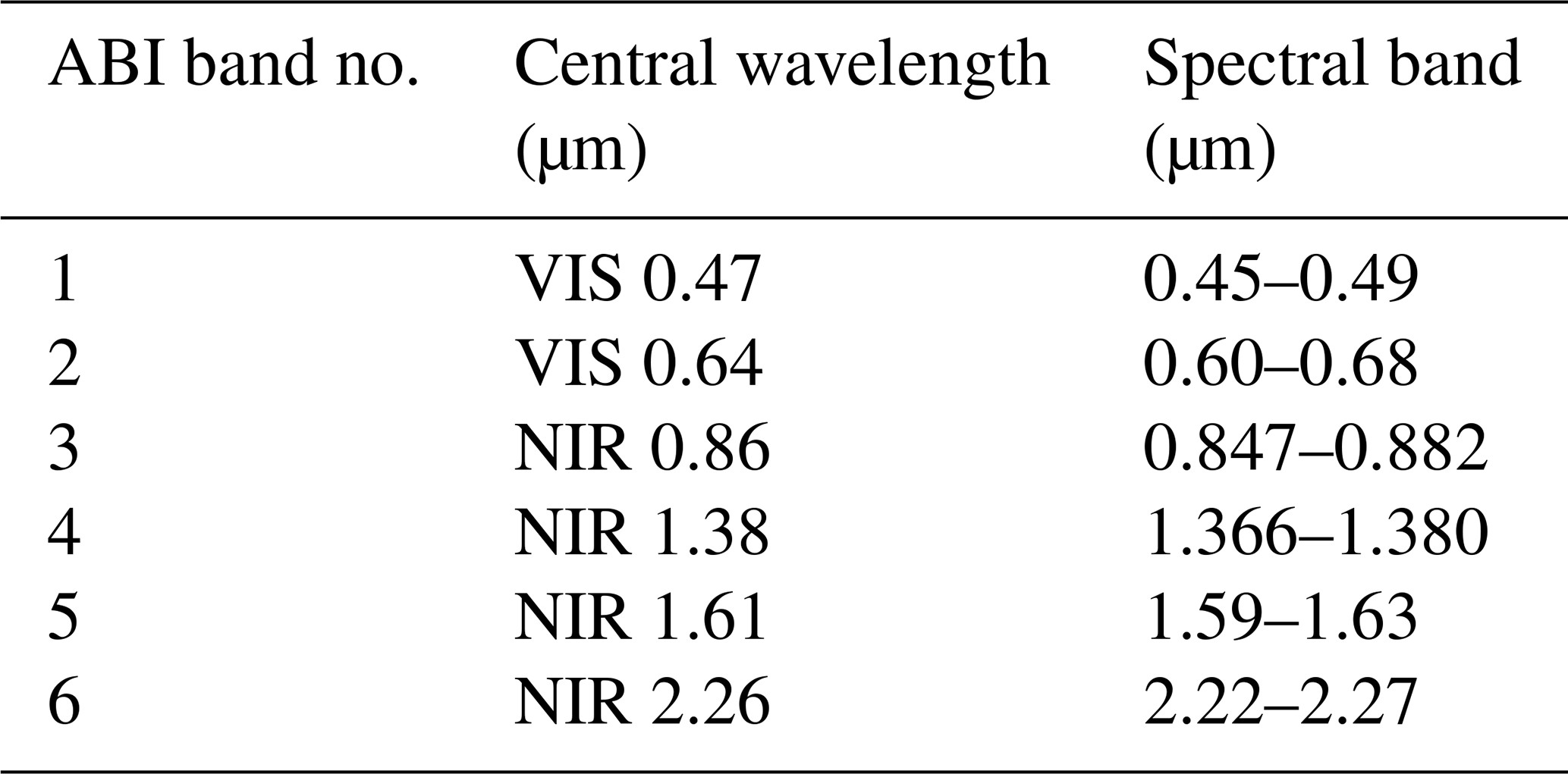
One of the objectives at NOAA/STAR with respect to the utilization of observations from the Advanced Baseline Imager (ABI) is to be able to derive shortwave (SW↓) radiative fluxes at the surface. To get to the surface SW↓ from top-of-the-atmosphere (TOA) satellite observations, there are two generic approaches: (1) the direct approach and (2) the indirect approach. In the direct approach one uses all the necessary information needed for deriving the surface fluxes (some of which can be derived from satellites). Implementation of such an approach is feasible, for instance, with observations from MODIS, which has a long history of product availability and evaluation. Examples are illustrated in Wang and Pinker (2009), Niu and Pinker (2015), Ma et al. (2016), and Pinker et al. (2017a, b, 2018). GOES-R is a new instrument, and similar information as that from MODIS is not yet available. Therefore, the indirect approach is used when one starts from satellite observations at the TOA and models the atmosphere and surface with the best available information (which does not have to be based on ABI). Examples of such an approach are discussed in Pinker et al. (2005), Ma and Pinker (2012), and Zhang et al. (2019). The “indirect path method” is used at the Center for Satellite Applications and Research (STAR) (Laszlo et al., 2020) for deriving SW↓ radiative fluxes from satellite observations; it requires knowledge of the SW broadband (0.2–4.0 µm) top-of-the-atmosphere (TOA) albedo. The Advanced Baseline Imager (ABI) observations on board the NOAA GOES-R series of satellites provide reflectance in six narrow bands in the shortwave spectrum (Table 1); these must first be transformed into broadband reflectance (the NTB conversion), and the broadband reflectance must be transformed into a broadband albedo (the ADM conversion). During the pre-launch activity NTB transformations were developed based on theoretical radiative transfer simulations with MODTRAN 3.7 and 14 land use classifications from the International Geosphere–Biosphere Programme (IGBP) (Hansen et al., 2010). They were augmented with ADMs from (CERES) observed ADMs (Loeb et al., 2003) and theoretical simulations (Niu and Pinker, 2012) to compute TOA fluxes. The resulting NTB transformations and ADMs have been tested using proxy data and simulated ABI data. The proxy instruments used in these early simulations include the GOES-8 satellite, the Advanced Very High-Resolution Radiometer (AVHRR) sensor on the polar-orbiting satellites, the Spinning Enhanced Visible Infrared Imager (SEVIRI) sensor on the European METEOSAT Second Generation (MSG) satellites, and the Moderate Resolution Imaging Spectroradiometer (MODIS) instrument on the NASA Terra and Aqua polar-orbiting satellites. For each of these satellites, the evaluation of the methodologies was done differently; some results were evaluated against ground observations, while others were evaluated against TOA information from CERES as well as from the (ESA) Geostationary Earth Radiation Budget (GERB) satellite (Harries et al., 2005). The results obtained provided insight on the expected performance of the new ABI sensor. Those procedures have been subsequently updated and applied to the new ABI instrument once it was built and fully characterized.

Table 1 Channel information and spectral bands for ABI.

This is a first paper that describes the development of a methodology to derive TOA SW fluxes from the Advanced Baseline Imager on board the NOAA GOES-R series of geostationary satellites that are used at NOAA/STAR as a starting point for deriving surface SW↓ fluxes. Evaluation of the methodology against the best available estimates of TOA fluxes was also done. The TOA reflected SW flux is produced at NOAA together with the surface SW↓ flux and is archived at the NOAA Comprehensive Large Array-data Stewardship System (CLASS) at https://www.avl.class.noaa.gov (last access: 11 August 2022). While the TOA reflected SW flux is a product in its own right, it is also a prerequisite to deriving the SW↓ surface flux; as such, versions for TOA and the surface have the same labeling. The methodology will be presented in Sect. 2; the data used are described in Sect. 3, results in Sect. 4, and a summary and discussion in Sect. 5.

Figure 1 Flowchart of the NTB transformations illustrating the main processing sections.

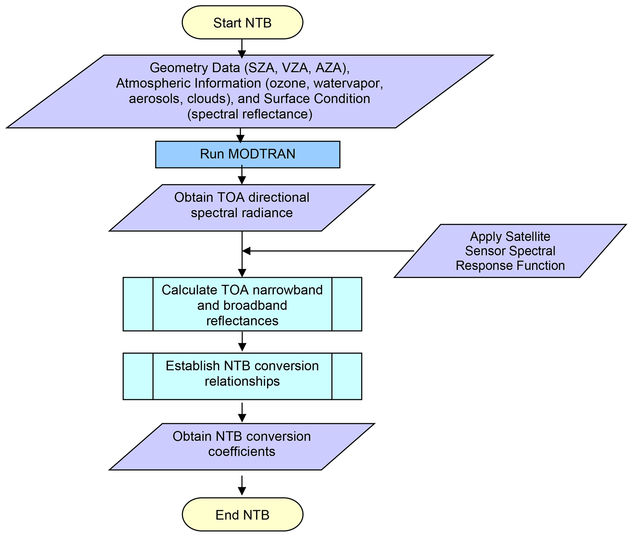
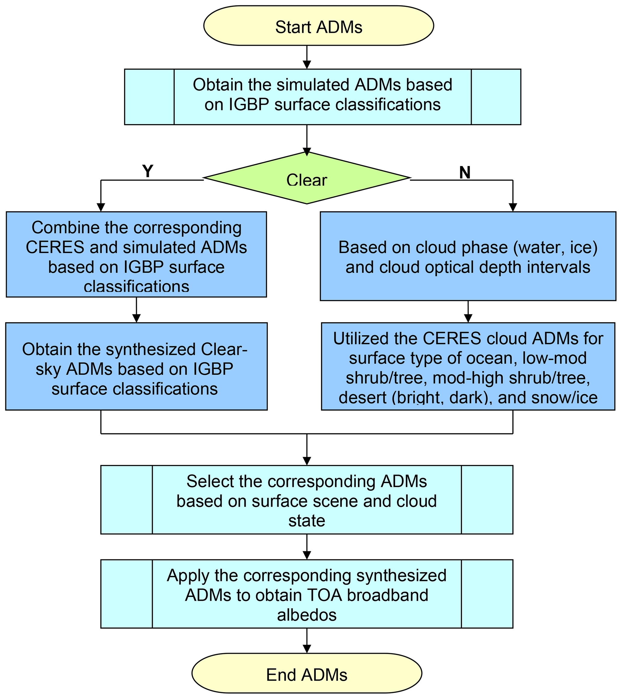
Figure 2 Schematic illustration of the logic employed to synthesize modeled and observed ADMs.

2 Methodology

The following two flowcharts (Figs. 1 and 2) describe the necessary steps to derive the NTB transformations and the ADMs. Details on these two steps will follow.

The TOA narrowband and broadband reflectance can be calculated from the spectral radiances simulated from MODTRAN 4.3 and the response functions of the satellite sensor as shown in Eqs. (1) and (2):

$$\begin{array}{}\text{(1)}& {\displaystyle }{\mathit{\rho }}_{\mathrm{nb}}({\mathit{\theta }}_{\mathrm{0}},\mathit{\theta },\mathit{\phi })={\displaystyle \frac{\mathit{\pi }\underset{\mathit{\lambda }\mathrm{1}}{\overset{\mathit{\lambda }\mathrm{2}}{\int }}I(\mathit{\lambda },{\mathit{\theta }}_{\mathrm{0}},\mathit{\theta },\mathit{\phi })G\left(\mathit{\lambda }\right)\mathrm{d}\mathit{\lambda }}{\underset{\mathit{\lambda }\mathrm{1}}{\overset{\mathit{\lambda }\mathrm{2}}{\int }}\cos \left({\mathit{\theta }}_{\mathrm{0}}\right)S_{\mathrm{0}}\left(\mathit{\lambda }\right)G\left(\mathit{\lambda }\right)\mathrm{d}\mathit{\lambda }}},\text{(2)}& {\displaystyle }{\mathit{\rho }}_{\mathrm{bb}}({\mathit{\theta }}_{\mathrm{0}},\mathit{\theta },\mathit{\phi })={\displaystyle \frac{\mathit{\pi }\underset{\mathrm{0.2}\mathrm{\mu }\mathrm{m}}{\overset{\mathrm{4}\mathrm{\mu }\mathrm{m}}{\int }}I(\mathit{\lambda },{\mathit{\theta }}_{\mathrm{0}},\mathit{\theta },\mathit{\phi })\mathrm{d}\mathit{\lambda }}{\underset{\mathrm{0.2}\mathrm{\mu }\mathrm{m}}{\overset{\mathrm{4}\mathrm{\mu }\mathrm{m}}{\int }}\cos \left({\mathit{\theta }}_{\mathrm{0}}\right)S_{\mathrm{0}}\left(\mathit{\lambda }\right)\mathrm{d}\mathit{\lambda }}},\end{array}$$

where ρ_nb is narrowband reflectance, ρ_bb is broadband reflectance, θ₀ is solar zenith angle, θ is the view (satellite) zenith angle, φ is the relative azimuth angle, I_λ is reflected spectral radiance, S₀(λ) is solar spectral irradiance, G_λ is the spectral response functions of satellite sensors, and λ₁ and λ₂ are the spectral limits of the sensor spectral band. This approach is widely used in the scientific community as also implemented in the work of Loeb et al. (2005), Wielicki et al. (2008), Su et al. (2015), Akkermans and Clerbaux (2020), and Clerbaux et al. (2009).

As stated previously, the ADMs from CERES-based observations (Loeb et al., 2005; Kato and Loeb, 2005; Kato et al., 2015) were augmented with theoretical simulations (Niu and Pinker, 2012) to compute TOA fluxes. This was done since CERES observations at that time were under-sampled at higher latitudes.

The combined ADMs are developed for each angular bin by weighting the modeled and CERES ADMs based on the number of samples used to derive the ADMs of each type (Niu and Pinker, 2012). Specifically,

$$\begin{array}{}\text{(3)}& \begin{array}{rl}\stackrel{\mathrm{‾}}{R}({\mathit{\theta }}_{\mathrm{0}},\mathit{\theta },\mathit{\phi })& ={\displaystyle \frac{\mathrm{1}}{m+n}}(m\times R_{\mathrm{CERES}}({\mathit{\theta }}_{\mathrm{0}},\mathit{\theta },\mathit{\phi })\\ & +n\times R_{\mathrm{S}}({\mathit{\theta }}_{\mathrm{0}},\mathit{\theta },\mathit{\phi })),\end{array}\end{array}$$

where $\stackrel{\mathrm{‾}}{R}({\mathit{\theta }}_{\mathrm{0}},\mathit{\theta },\mathit{\phi })$ represents averaged ADMs at each angular bin, R_CERES is the anisotropic factor from CERES ADMs, R_S is the anisotropic factor from simulated ADMs, and m and n are observation numbers at angular bins for CERES and simulated ADMs.

Figure 3 The location of the 100 selected clear-sky profiles from SeeBor used in the simulations.

2.1 Selection of atmospheric profiles for simulations

We have selected 100 atmospheric profiles covering the globe and the seasons as input for simulations with MODTRAN 4.3. The atmospheric profiles at each pressure level include temperature, water vapor, and ozone. Each season includes 25 profiles. A tool was developed to select profiles from a training dataset known as SeeBor Version 5.0 (https://cimss.ssec.wisc.edu/training_data/, last access: 11 August 2022) (Borbas et al., 2005). Originally it consisted of 15 704 global profiles of temperature, moisture, and ozone at 101 pressure levels for clear-sky conditions. The profiles are taken from NOAA-88 and the European Centre for Medium-Range Weather Forecasts (ECMWF) 60L training set, TIGR-3, ozonesondes from eight NOAA Climate Monitoring and Diagnostics Laboratory (CMDL) sites, and radiosondes from the Sahara during 2004. A technique to extend the temperature, moisture, and ozone profiles above the level of existing data was also implemented by the providers (University of Wisconsin-Madison, Space Science and Engineering Center, Cooperative Institute for Meteorological Satellite Studies (CIMSS). Figure 3 shows the location of the selected profiles.

The SeeBor profiles are clear-sky profiles. The top of the profiles is at 0.005 mb, which is about 82.6 km. We did an experiment to check the impact of reducing the number of levels for a profile (initially, we used only 40 levels). In the experiment radiances were computed from profiles with 50 levels as were radiances from profiles with 98 levels. The difference between the two radiances (50 lev–98 lev) was below 5 %, reaching 15 % around 2.5 µm. In the experiment we used the odd number levels starting from surface (plus the highest level) to reduce the number of profile levels. Based on these experiments we have opted to keep all 98 profile levels.

The surface variables we have used are from MODIS and include surface skin temperature, 2 m temperature, land–sea mask, and albedo. We have conducted a thorough investigation of how the selected profiles represent the entire sample of 15 704 profiles. An example comparison of temperature, humidity, and ozone profiles is shown in Fig. 4. As seen, there is a positive bias in the selected profile of temperature due to their higher concentration at the lower latitudes. A positive bias can be found at the lower levels, while a negative bias is seen above 1 mb. Since our domain of study is in such latitudes this selection should not have adverse effects on the simulations performed.

Table 2 Surface classification description for IGBP 18 types, IGBP 12 types, CERES clear sky 6 types, and NTB cloudy sky 4 types.

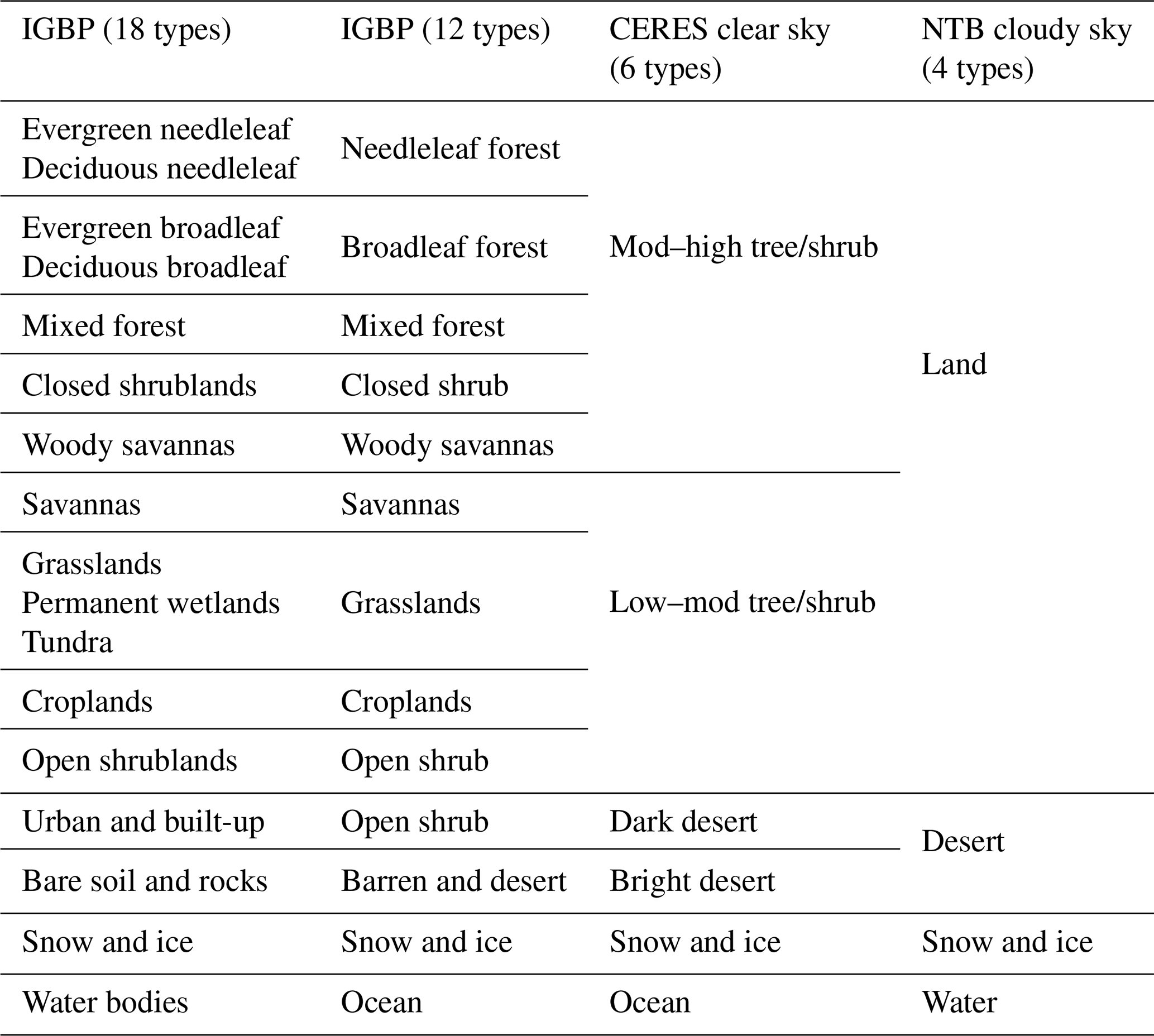
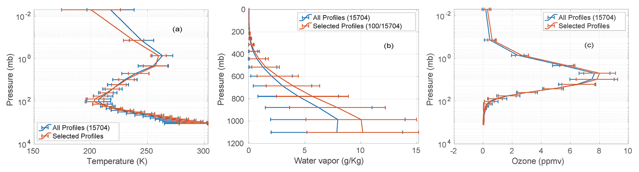
Figure 4 Profile statistics of (a) temperature, (b) water vapor, and (c) ozone for the entire available sample and for the reduced sample used in this study. The error bar is 1 standard deviation.

2.2 Surface conditions

The surface condition is one of the primary inputs into the MODTRAN simulations. The International Geosphere–Biosphere Programme (IGBP) land classification is used as a source (Hansen et al., 2010; Loveland et al., 2010). The dataset is at $\mathrm{1}/\mathrm{6}$^∘ resolution and includes 18 surface types. We have converted the $\mathrm{1}/\mathrm{6}$^∘ (∼18.5 km) resolution to the ABI 2 km grid using the nearest grid method (Fig. 5). The surface type is fixed in time. The method for cloudy sky uses 4 surface types; these are also derived from 12 IGBP types (Table 2).

Figure 5 Re-mapped IGBP surface classifications over CONUS on the 2 km ABI grid.

Table 3 The various classes for which NTB coefficients are generated.

2.3 Clear- and cloudy-sky simulations

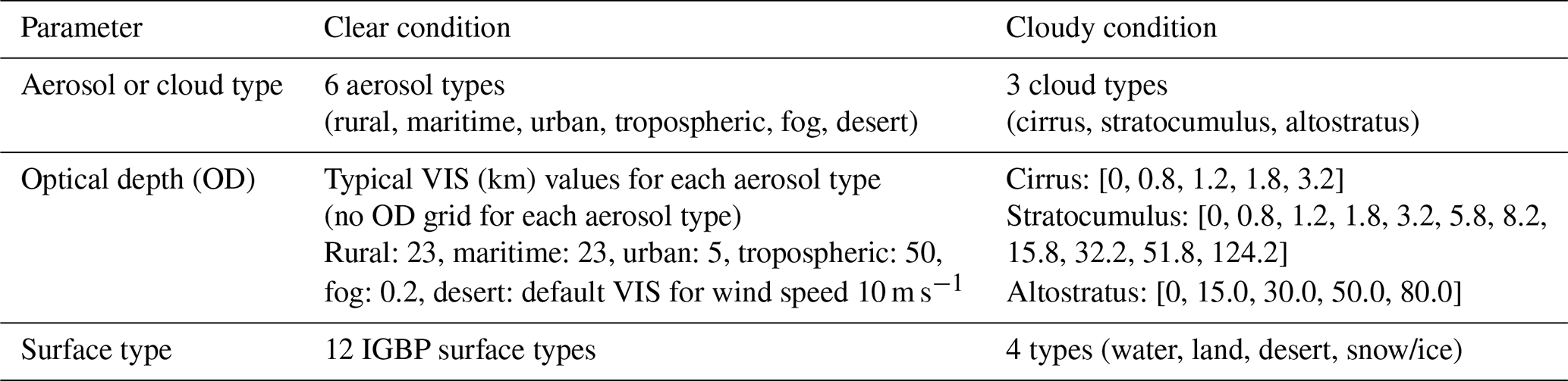
Under clear sky, scattering from aerosols is important. We have included six aerosol types (Table 3) to cover a range of possible conditions under clear sky. Aerosol models are selected based on the type of extinction and a default meteorological range for the boundary layer aerosol models as listed below.

• Aerosol type 1: rural extinction, visibility 23 km

• Aerosol type 4: maritime extinction, visibility 23 km

• Aerosol type 5: urban extinction, visibility 5 km

• Aerosol type 6: tropospheric extinction, visibility 50 km

• Aerosol type 8: advective fog extinction, visibility 0.2 km

• Aerosol type 10: desert extinction for default wind conditions

For the six aerosol types, the total number of MODTRAN simulations for each surface type is 462 000. It is obtained as follows: 6 aerosol types ×100 profiles ×770 angles.

When performing NTB simulations, we use all six types of aerosols. The rural, ocean, urban, and fog aerosols are distributed in the lower 0–2 km region. Tropospheric aerosol is distributed from 0 to the 10 km tropopause. The rural, ocean, urban, and tropospheric aerosol optical properties have relative humidity (RH) dependency. The single-scattering albedo (SSA) is given on four RH grids (0, 70, 80, 99) on a spectral grid of 788 points ranging from 0.2 to 300 µm.

Simulations were performed for ABI for all the cloud cases described in Table 3. To merge cloud layers with atmospheric profiles we have followed the procedure as described in Berk et al. (1985, 1998), namely the following: “Cloud profiles are merged with the other atmospheric profiles (pressure, temperature, molecular constituent, and aerosol) by combining and/or adding new layer boundaries. Any cloud layer boundary within half a meter of an atmospheric boundary layer is translated to make the layer altitudes coincide; new atmospheric layer boundaries are defined to accommodate the additional cloud layer boundaries”. 100 % relative humidity is assumed within the cloud layers (default).

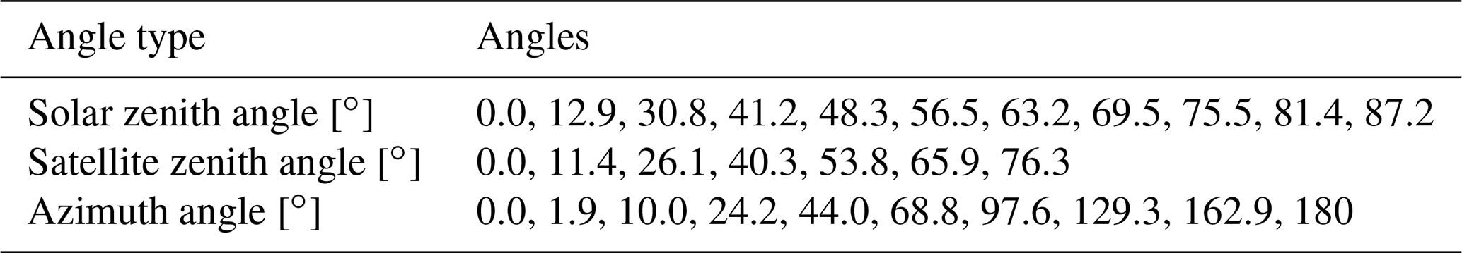
Table 4 Angles used in simulations. To be consistent with what is presented in the ABI Shortwave Radiation Budget (SRB) Algorithm Theoretical Basis Documents (ATBD) (Laszlo et al., 2018) the additional angles used in the simulations are not given in this table.

2.4 Selection of angles

The total number of angles used in the simulations is given in Table 4. The selected spectral grids for solar zenith angles, satellite view angles, and relative azimuth angles are at Gaussian quadrature points, plus 0^∘ to solar zenith angles (SZAs) and satellite viewing angles (VZAs) as well as 0 and 180^∘ (forward and backward view) to the satellite relative azimuth angles. Solar angle and satellite view angle are referenced to the target or surface for satellite simulations with 0^∘, meaning looking up (zenith). Relative azimuth angle is defined as when the relative azimuth angle equals 180^∘, and the sun is in front of the observer.

The definitions of solar zenith angle and azimuth angle in this table correspond to the definitions of MODTRAN, but that is not the case for the satellite zenith angle. MODTRAN uses the nadir angle as the 180^∘ satellite zenith angle, ignoring spherical geometry.

2.5 Selection of optimal computational scheme

MODTRAN 4.3 provides three multiple-scattering models (Isaacs, DISORT, and scaled Isaacs) and three band models at resolutions of 1, 5, and 15 cm⁻¹. The DISORT model (Stamnes et al., 1988) provides the most accurate radiance simulations, but the runs are very time-consuming. The Isaacs (Isaacs et al., 1987) two-stream algorithm is fast but oversimplified. The scaled Isaacs method performs radiance calculations using the Isaacs two-stream model over the full spectral range and using the DISORT model at a small number of atmospheric window wavelengths. The multiple-scattering contributions for each method are identified, and ratios of the DISORT and Isaacs methods are computed. This ratio is interpolated over the full wavelength range and finally applied as a multiple-scattering scale factor in a spectral radiance calculation performed with the Isaacs method.

To optimize simulation speed and accuracy, we performed various sensitivity tests, including combinations of multiple-scattering models, band resolution, and number of streams. Table 5 lists simulation options and their corresponding calculation speed.

Table 5 MODTRAN simulation speed test (CPU MHz 2099.929).

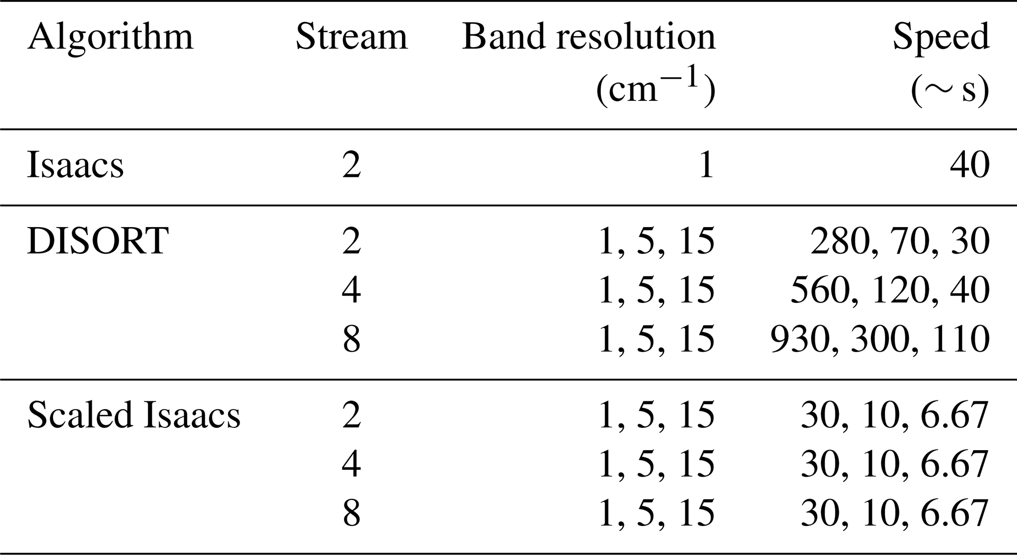
Based on results presented in Table 5, the efficient options (<40 s) are Isaacs, DISORT two-stream with 15 cm⁻¹, DISORT four-stream 15 cm⁻¹, and scaled Isaacs all streams at all resolutions. Although the ideal option is DISORT eight-stream with 1 cm⁻¹ resolution, there is a trade-off between speed and accuracy. Figure 6 compares DISORT-simulated radiances at three band resolutions. We use two spectral ranges of 0.4–0.5 and 1.5–2.0 µm to illustrate differences. Figure 6 shows that the coarser band resolution has smoothed out the radiance variations. The 15 cm⁻¹ has the smoothest curve among the three, and 1 cm⁻¹ shows more variations than the other two. Another (scientific) criterion for selecting the spectral resolution is the ability to resolve and/or match the relative spectral response function (SRF) of a sensor. For example, the SRFs of channels 1–6 of ABI are given every 1 cm⁻¹.

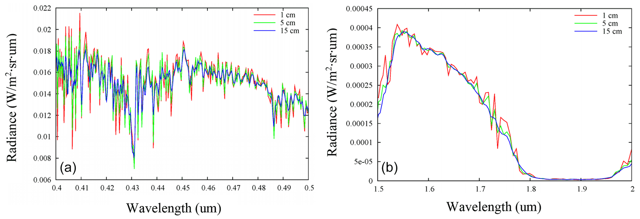
Figure 6 Simulated radiances from the DISORT eight-stream (with 1, 5, and 15 cm⁻¹ resolution) band model for a spectral range of 0.4–0.5 µm (a) and 1.5–2.0 µm (b).

Accordingly, we have chosen the 1 cm⁻¹ band model for the MODTRAN radiance simulations. Radiance simulations from different multiple-scattering models at 1 cm⁻¹ resolution were also performed. The whole spectrum of 0.2–4 µm was separated into 14 sections so that the differences can be assessed clearly. For wavelengths below 0.3 µm and beyond 2.5 no discernible differences were found among Isaacs, DISORT two-, four-, and eight-stream, and scaled Isaacs. The largest differences occurred in the spectral range of 0.4–1.0 µm. Scaled Isaacs eight-stream follows DISORT eight-stream closely across the whole spectral range; the scaled Isaacs method provided near-DISORT accuracy with the speed of Isaacs. Thus, the MODTRAN 4.3 simulations for GOES-R ABI were set up with scaled Isaacs eight-stream with 1 cm⁻¹ band resolution.

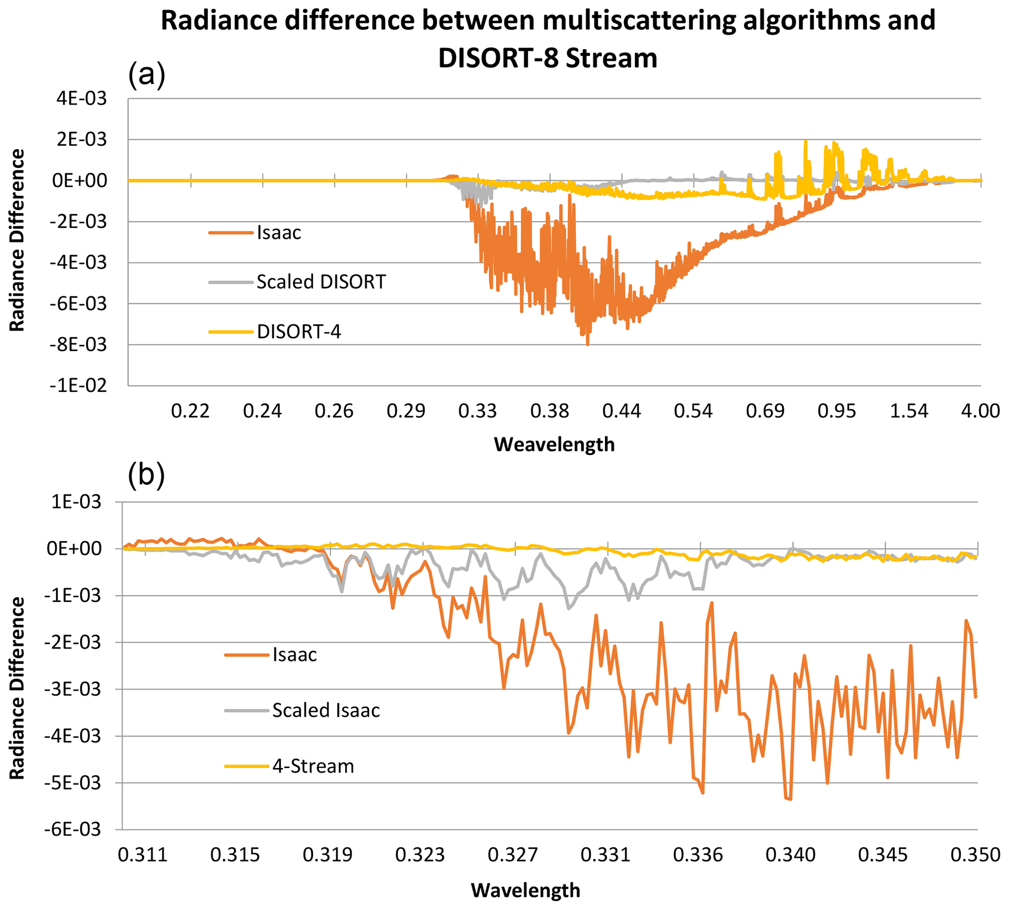
Figure 7 Radiance differences between various multi-scattering algorithms and DISORT eight-stream. (a) The whole simulated spectrum of 0.2–4 µm. (b) Zoom on 0.3–0.35 µm (relative azimuthal angle 1.9^∘, view angle 76.3^∘, and solar zenith angle 87.2^∘).

For illustration, in Fig. 7 radiances simulated by Isaacs two-stream, scaled Isaacs, and DISORT four-stream are compared for the case of a relative azimuthal angle of 1.9^∘, a view angle of 76.3^∘, and a solar zenith angle of 87.2^∘. The lines are differences between various settings and DISORT eight-stream (e.g., Isaacs minus DISORT-8). The Isaacs method has the least accuracy since it is oversimplified; four-stream showed some improvements when compared with Isaacs, while it still has large differences for 0.4 µm and is still computationally demanding. Scaled Isaacs provides the smallest differences from DISORT-8. Figure 7 (lower) is zoomed in to the large difference area of 0.3–0.35 µm, which indicates that scaled Isaacs still provides satisfactory results.

2.6 Regression methodologies

We have derived coefficients of regression using a constrained least-square curve-fitting method of MATLAB, “lsqnonneg”, which can solve a linear or nonlinear least-squares (data-fitting) problem and produce non-negative coefficients. Non-negative coefficients avoid generating negative TOA flux, which is not a physically valid.

To ensure that information from all channels is used and avoid the complex cross-correlation problem, it was opted to generate narrow-to-broad (NTB) coefficients for each ABI channel separately. These channel-specific NTB coefficients are applied to each channel to convert ABI narrowband reflectance to extended band. The final broadband TOA reflectance is taken as the weighted sum of the broadband reflectances of all six specific channels. The logic behind this approach is the assumption that the narrowband reflectance from each channel is a good representative for a limited spectral region centered around the channel and the total spectral reflectance is dominated by the spectral region that contains the most solar energy.

To generate “separate-channel” NTB coefficients, each narrowband ABI channel reflectance is converted to a reflectance ρ_bb,i separately,

$$\begin{array}{}\text{(4)}& {\mathit{\rho }}_{\mathrm{bb},i}\left({\mathit{\theta }}_{\mathrm{0}}\mathit{\theta }\mathit{\varphi }\right)=c_{\mathrm{0},i}\left({\mathit{\theta }}_{\mathrm{0}}\mathit{\theta }\mathit{\varphi }\right)+c_{\mathrm{1},i}\left({\mathit{\theta }}_{\mathrm{0}}\mathit{\theta }\mathit{\varphi }\right)\times {\mathit{\rho }}_{\mathrm{nb},i}\left({\mathit{\theta }}_{\mathrm{0}}\mathit{\theta }\mathit{\varphi }\right),\end{array}$$

where ρ_bb,i is the band reflectance for an interval around each channel i, and c_0,i and c_1,i are regression coefficients for channel i. These regression coefficients are derived separately for various combination of surface, cloud, and aerosol types. The total shortwave broadband (0.25–4.0 µm) reflectance ${\mathit{\rho }}_{\mathrm{bb}}^{\mathrm{est}}$ is obtained by taking the weighted sum of all six ρ_bb,i reflectances.

$$\begin{array}{}\text{(5)}& {\mathit{\rho }}_{\mathrm{bb}}^{\mathrm{est}}\left({\mathit{\theta }}_{\mathrm{0}}\mathit{\theta }\mathit{\varphi }\right)={\sum }_i{\mathit{\rho }}_{\mathrm{bb},i}({\mathit{\theta }}_{\mathrm{0}},\mathit{\theta },\mathit{\varphi }){\displaystyle \frac{S_{\mathrm{0},i}}{S_{\mathrm{0}}}}\end{array}$$

Here, S₀ and S_0,i are total solar irradiance and band solar irradiance for each channel, respectively. Band edges around the six ABI channels are 49 980–18 723, 18 723–13 185, 13 185–9221, 9221–6812, 6812–5292, and 2500 cm⁻¹ (0.2001–0.5341, 0.5341–0.7584, 0.7584–1.0845, 1.0845-1.4680, 1.4680–1.8896, and 1.8896–4.0000 µm). The corresponding solar irradiance band values are 364, 360, 287, 168, 91, and 87 W m⁻². Figure 8 shows the sensor response function (SRF) and locations of the six ABI channels.

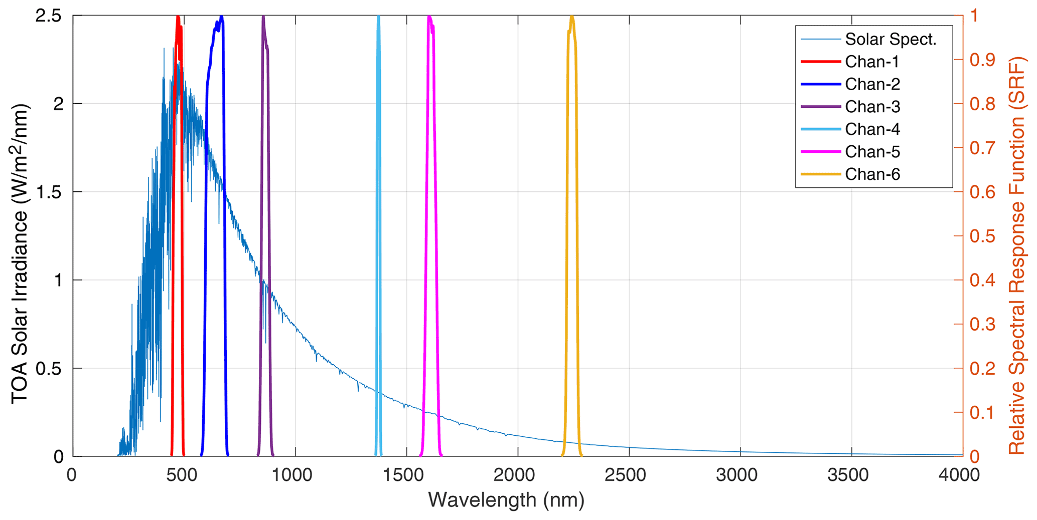
Figure 8 Locations of the six ABI channel SRFs. The x axis is the wavenumber. The y axis is solar irradiance.

Coefficients are generated for clear conditions and three types of cloudy conditions. Comparison between ABI TOA flux and CERES products is shown in Fig. 9. The separate-channel coefficients work well for predominantly clear sky (Fig. 10). Differences are somewhat more scattered for cloudy cases. The reason may be due to the fact that the ABI observation time and CERES product time do not match perfectly since cloud conditions change quickly. As discussed in Gristey et al. (2021) there are SW spectral reflectance variations for different cloud types. Possibly, for ABI bands some spectral variations associated with cloud variability are missed. It is important to have the correct cloud properties to be able to select the correct ADM. Misclassification of cloud properties will therefore result in flux differences. They also argue that ADMs have an uncertainty due to within-scene variability and within-angular-bin variability, leading to additional flux differences. Spectral band difference adjustment factors (Scarino et al., 2016) can also be used to account for differences.

Table 6 Details on data used as input for calculations.

^* The CODC data were not always available from CLASS and had to be obtained from NOAA/STAR temporary archives. Also, not all the required angular information needed for implementation of the regressions is available online and had to be re-generated.

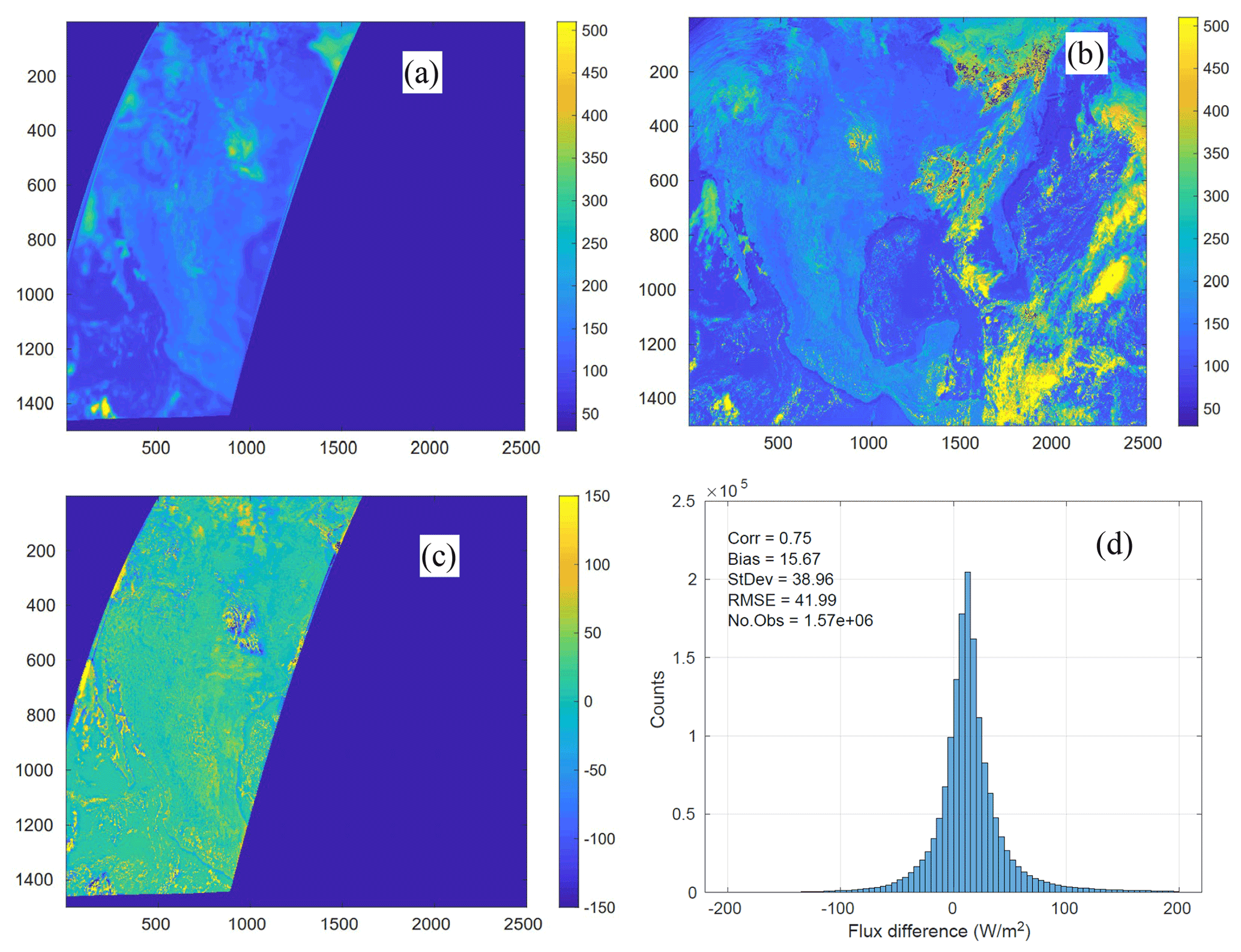
Figure 9 Comparison of TOA SW flux from ABI and CERES FLASHFlux for 25 November 2017 at 17:57 Z: (a) CERES FLASHFlux Terra product, (b) results from ABI with “separate-channel” coefficients, (c) difference of ABI–CERES FLASHFlux, and (d) histogram of ABI–CERES FLASHFlux differences (this is the only case illustrated in this paper with data from FLASHFlux; Kratz et al., 2014).

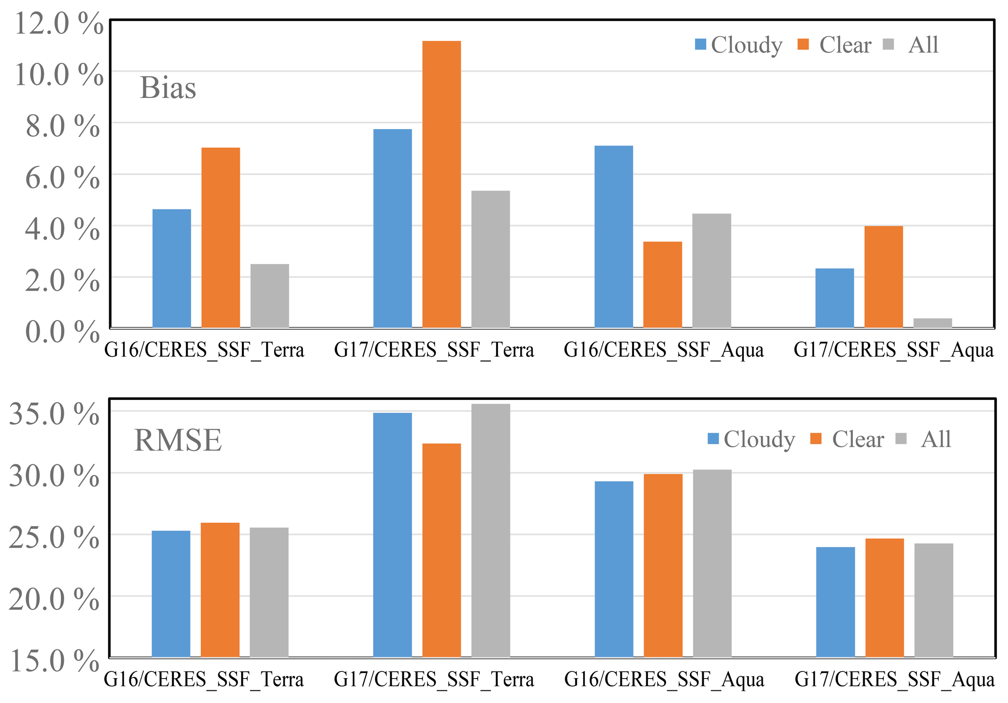
Figure 10 Statistics for relative bias and root mean square error (RMSE). The y axis is percentage. The x axis is the case used in the intercomparison. Blue – cloudy, orange – clear sky, and gray – all sky.

3 Data used

3.1 Satellite data for GOES-16 and GOES-17

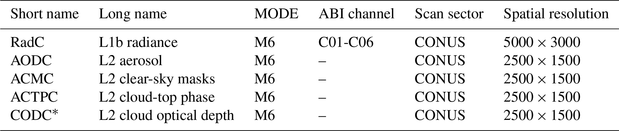
The Advanced Baseline Imager (ABI) data used (Table 6) were downloaded from the NOAA Comprehensive Large Array-data Stewardship System (CLASS) at https://www.avl.class.noaa.gov/saa/products/welcome (last access: 11 August 2022). Both level 1b (L1b) and level 2 (L2) data were used. These can be found by searching the CLASS site by selecting “GOES-R Series ABI Products GRABIPRD (partially restricted L1b and L2+ Data Products)”. The L1b data included the radiances (RadC) in files “OR_ABI-L1b-RadC-MmCnn_G1SS_stime_etime_ctime”, where “m”, “nn”, and “SS” indicate the ABI scan mode, channel number (01–06), and satellite identification number (16 or 17), respectively. The notations “stime” and “etime” are the start and end dates and times of the scan, and “ctime” is the date and time the file was created. The ABI L2 products used were the clear-sky mask, cloud-top phase, and cloud optical depth. The names of these files are constructed similarly to the L1b radiance files, except that the radiance product name RadC is replaced by ACMC, ACTPC, CODC, and AODC, respectively, and the reference to the channel number is omitted. For example, for GOES-16 with ABI operating in scan mode 6 in the CONUS domain, the name of the clear-sky mask file is OR_ABI-L2-ACMC-M6_G16_stime_etime_ctime. (In the product names above the letter C indicates the CONUS domain.)

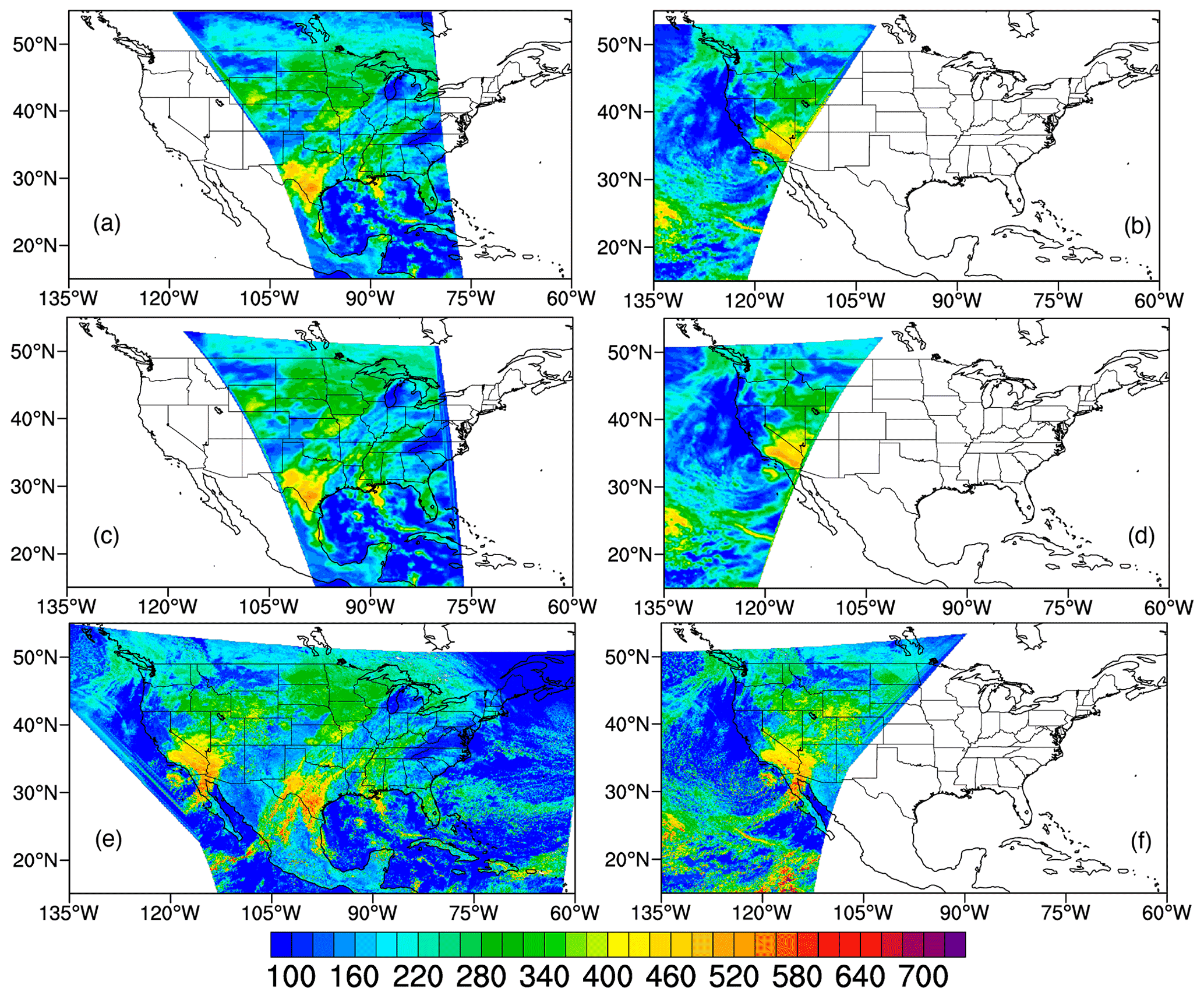
Figure 11 All-sky TOA SW from (a) CERES_SSF/Aqua, (b) CERES_SSF/Terra, (c) re-gridded CERES_SSF/Aqua, (d) re-gridded CERES_SSF/Terra, (e) GOES-16, and (f) GOES-17: all on 26 December 2019 at 19:36 UTC.

The clear-sky mask product consists of a binary cloud mask identifying pixels as clear, probably clear, cloudy, or probably cloudy. The cloud-top phase product provides cloud classification identification information for each pixel. The cloud phase categories are clear sky, liquid water, super-cooled liquid water, mixed phase, ice, and unknown. The cloud optical depth product gives the optical thickness along an atmospheric column for each pixel. All products have a nominal sub-satellite spatial resolution of 2 km.

When searching the NOAA CLASS site, go to “GOES-R Series ABI Products GRABIPRD (partially restricted L1b and L2+ Data Products)”. The SRFs are downloaded from https://ncc.nesdis.noaa.gov/GOESR/ABI.php (last access: 11 August 2022).

Table 7 Statistical summary for all selected cases intercompared at an instantaneous timescale.

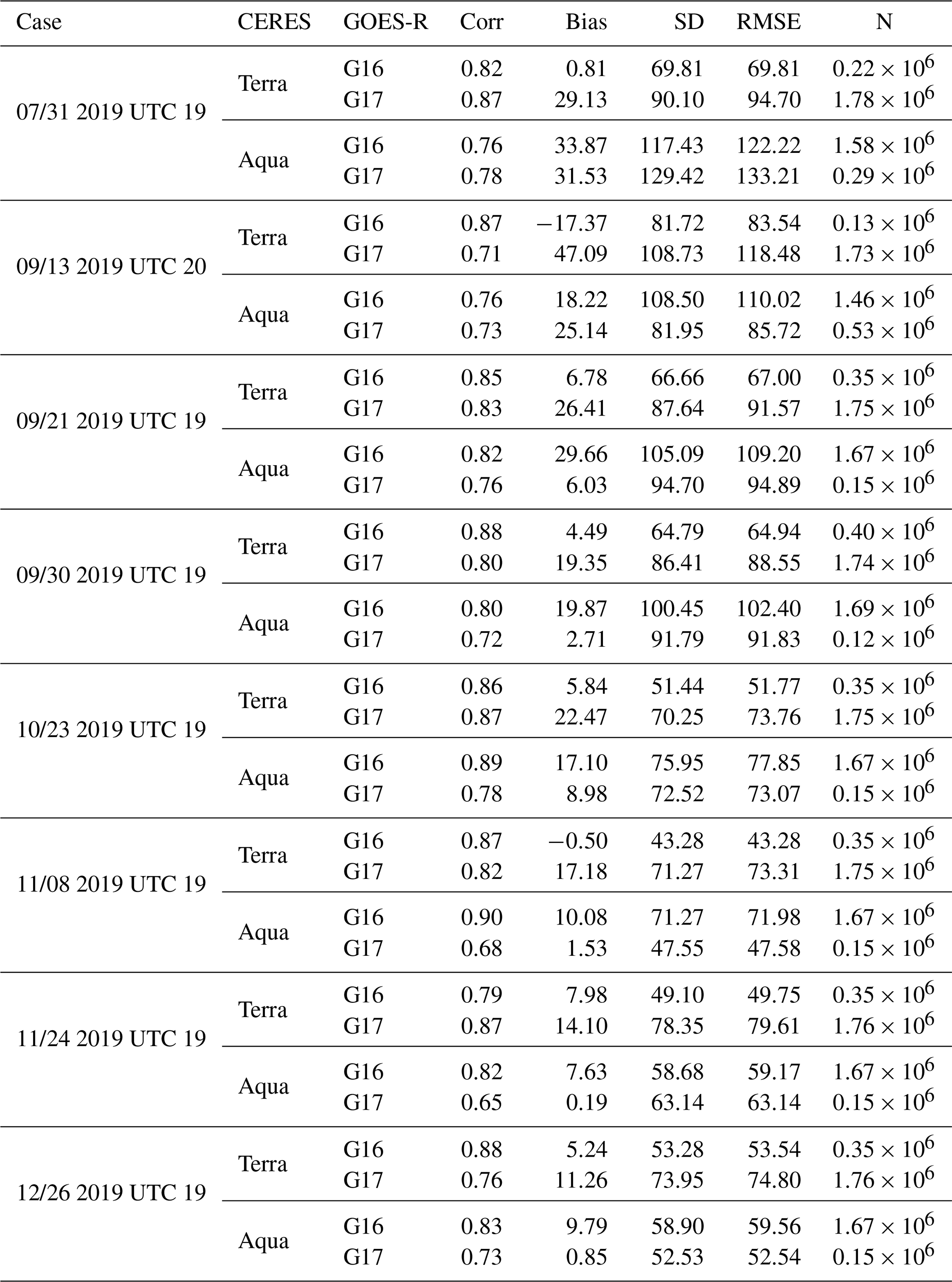
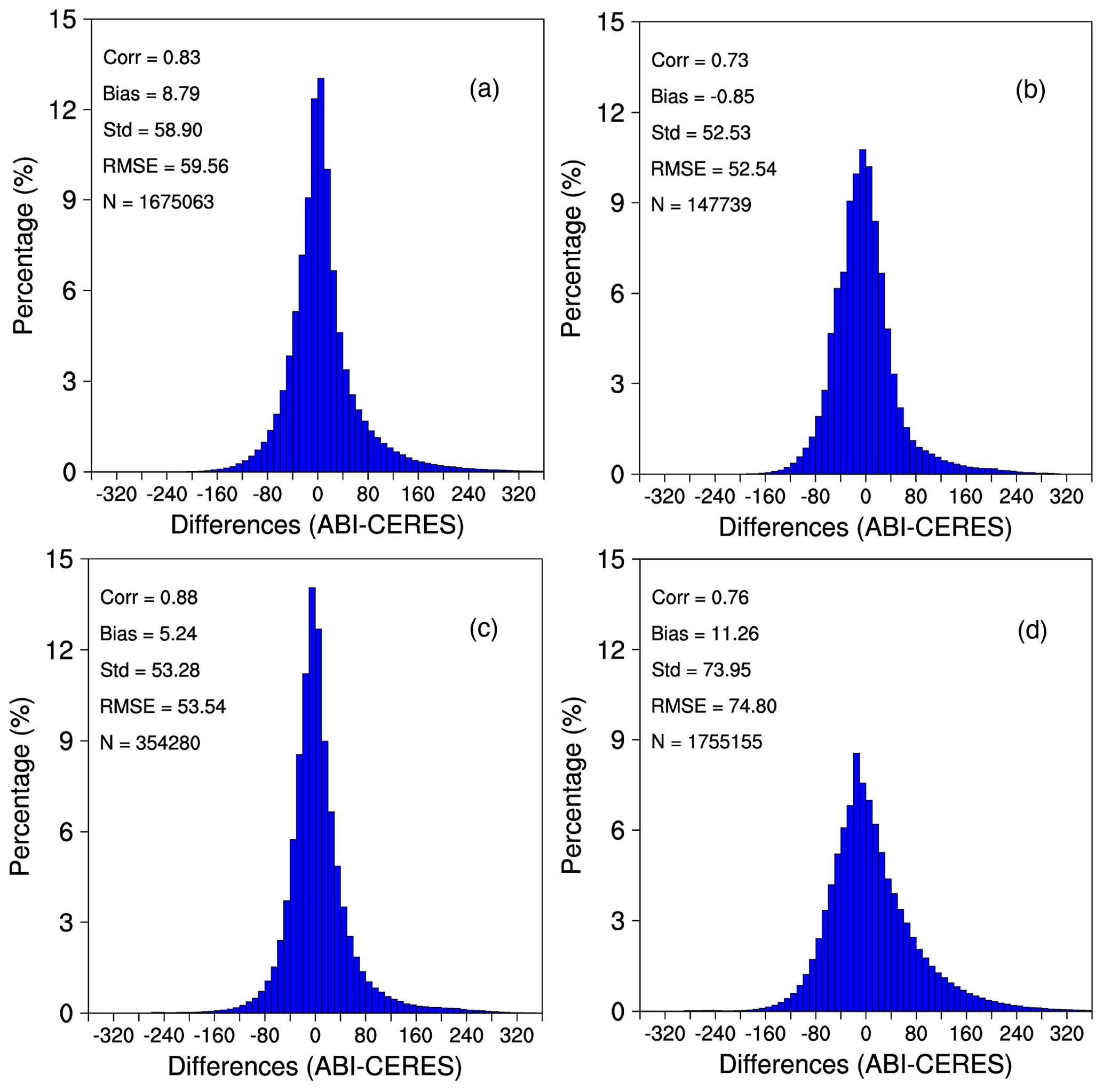
Figure 12 Frequency distribution of all-sky TOA SW differences between (a) ABI on GOES-16 and CERES_SSF using Aqua and between (b) ABI on GOES-17 and CERES_SSF using Aqua. (c) The same as (a) using Terra and (d) the same as (b) using Terra. All observations were used (clear and cloudy) on 26 December 2019 at 19:36 UTC.

Figure 13 Same as Fig. 11 but for clear TOA SW differences.

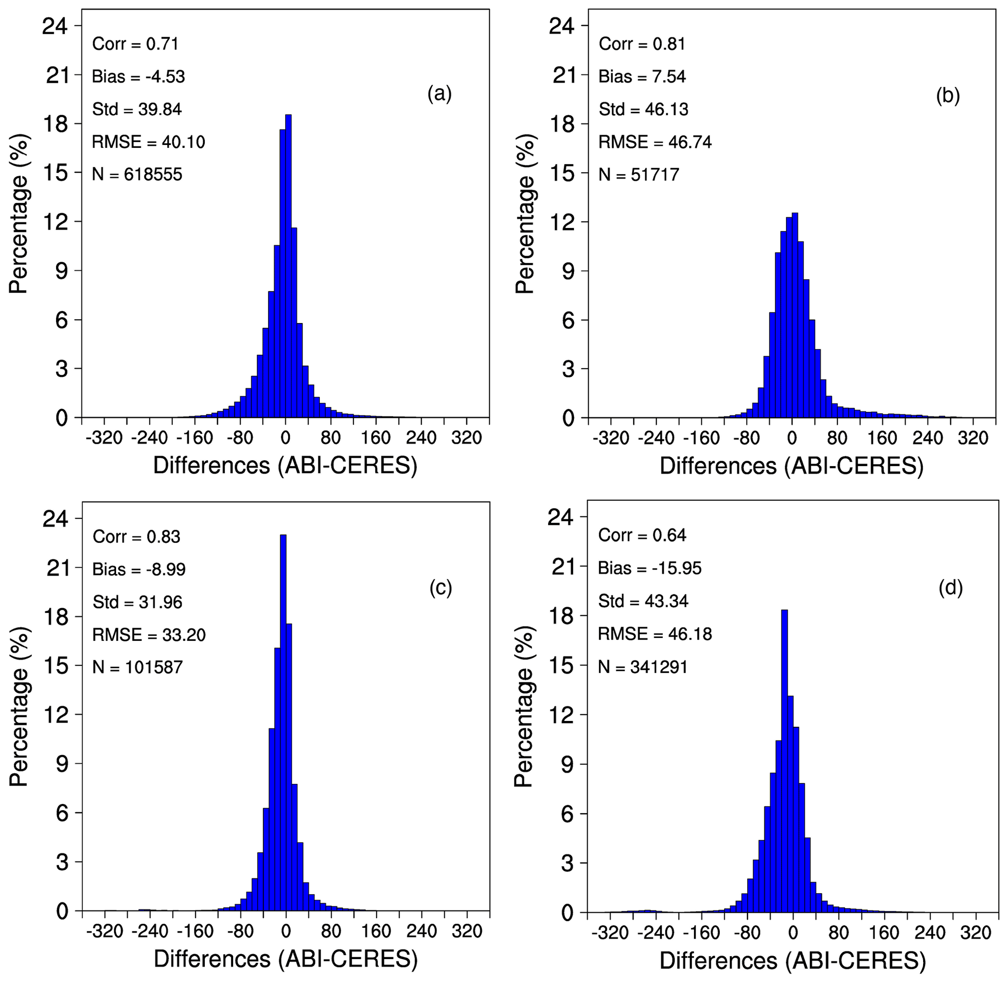
3.2 Reference data from CERES

The CERES Single-Scanner Footprint (SSF) is a unique product for studying the role of clouds, aerosols, and radiation in climate. Each CERES footprint (nadir resolution 20 km equivalent diameter) on the SSF includes reflected shortwave (SW), emitted longwave (LW), and window (WN) radiances as well as top-of-atmosphere (TOA) fluxes from CERES with temporally and spatially coincident imager-based radiances, cloud properties, and aerosols, along with meteorological information from a fixed four-dimensional analysis provided by the Global Modeling and Assimilation Office (GMAO). Each file in this data product contains 1 h of full- and partial-Earth view measurements or footprints at a surface reference level. Detailed information can be found via https://ceres.larc.nasa.gov/data/{#}ssf-level-2 (last access: 11 August 2022) (we used version 4a)

Near-real-time CERES fluxes and clouds in the SSF format are available within about a week of observation (Kratz et al., 2014). They do not use the most recent CERES instrument calibration and thus contain some uncertainty. Before GOES data were transferred to the Comprehensive Large Array-data Stewardship System (CLASS) system, the NOAA/STAR archive held new data for about a week. Therefore, the initial evaluations had to be done only with data that overlapped in time. The CERES data known as the FLASHFlux level 2 (FLASH_SSF) are available almost in real time from https://ceres.larc.nasa.gov/products.php?product=FLASHFlux-Level2 (last access: 11 August 2022) (we used version 3c).

Due to such constraints the early comparison was done between ABI data as archived at NOAA/STAR and the FLASHFlux products (in this paper, the FLASHFlux data were used only in Fig. 9). The archiving of GOES-R at the NOAA Comprehensive Large Array-data Stewardship System (CLASS) started only in 2019; however, it contains data starting from 2017. Once the CLASS archive became available, we augmented GOES-16 cases with observations from GOES-17; only those cases will be shown in this paper.

Figure 14 Same as Fig. 11 but for cloudy TOA SW differences.

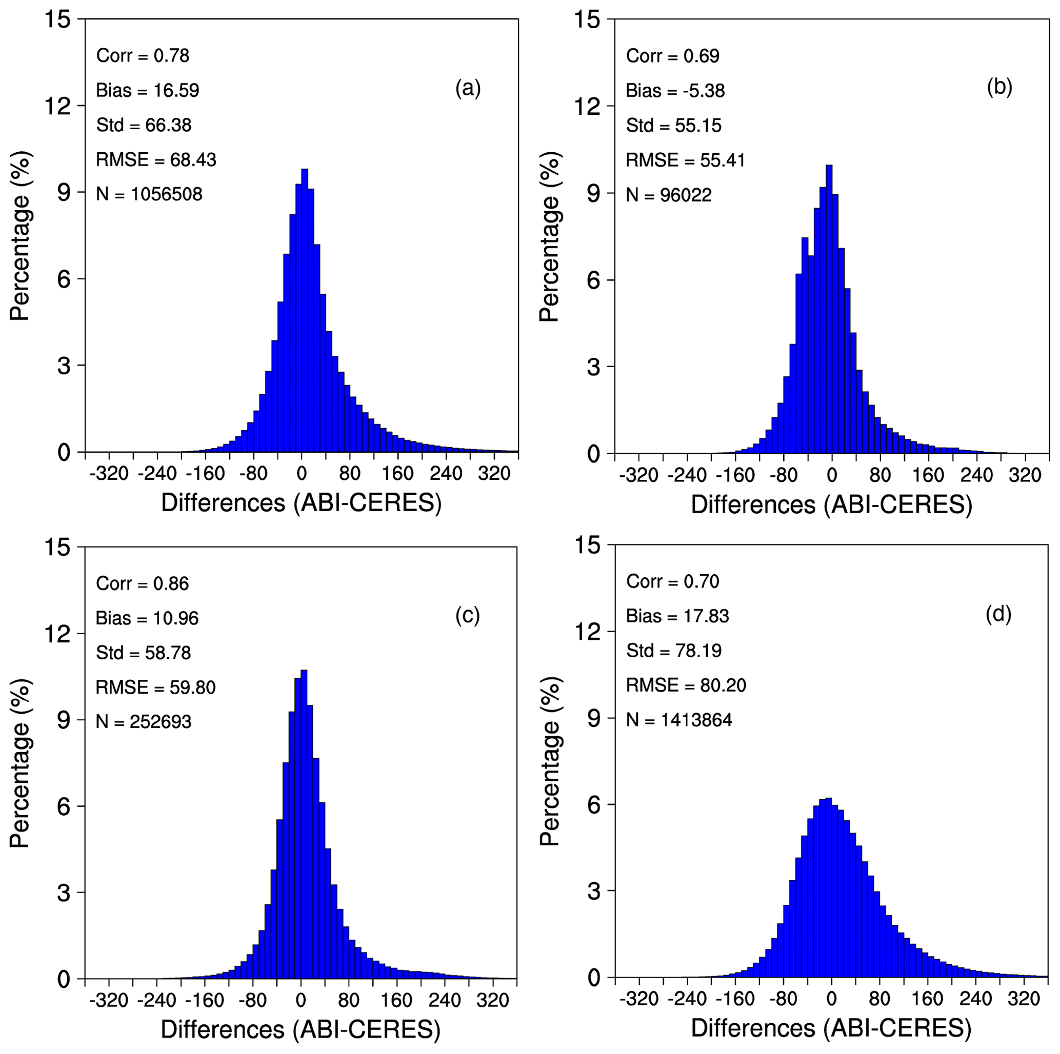
Figure 15 (a) Sensor response function for ABI channel 6; (a) spectral albedo for desert and open shrubs. The desert albedo value is much higher than open shrubs at 2.2 µm.

3.3 Data preparation

For the re-mapping, we adopted the ESMF re-gridding package. The detailed information can be found at http://earthsystemmodeling.org/regrid/ (last access: 11 August 2022).

For an ideal situation, the ABI high-resolution TOA SW fluxes should be mapped into the CERES footprint for validation. However, there are reasons that make it difficult to do so. There can be more than 18 000 pixels in a single swath of the SSF when constrained to the US. Different pixels have different times. Neglecting the seconds, there are still more than 30 min differences (this changes case by case) between the first pixel and the one at the end, and this brings up a time-matching issue. By re-mapping the SSF to ABI, we can set up a unique time for ABI (ABI is at 5 min intervals) and then constrain the region and the time range of SSF.

Both re-mapping the ABI to SSF and re-mapping SSF to the ABI bring up spatial matching errors as recognized by the scientific community (Rilee and Kuo, 2018; Ragulapati et al., 2021). In Fig. 11, we show the SSF before re-gridding (Fig. 11a and b) and after re-gridding (Fig. 11c and d). The fluxes after re-mapping CERES SSF to the ABI resolution resemble the original structure well. Another consideration is the computational efficiency of re-mapping the curvilinear tripolar grid to an unconstructed grid. For large arrays, it is more efficient to re-map the unconstructed grid to the curvilinear tripolar grid.

4 Results

4.1 Comparison between ABI TOA fluxes and those from CERES SSF

A case for 26 December 2019 (doy 360) at 19:36 UTC is illustrated in Figs. 11–14. Statistical summaries from an extended number of cases that cover all four seasons are presented in Table 7.

We have conducted several experiments to select an appropriate regression approach to the NTB transformation, ensuring that nonphysical results are not encountered. Based on the samples used in this study (Table 7) the differences found for Terra and GOES-16 were in the range of −0.5–(−17.37) for bias and 43.28–81.72 for standard deviation; for Terra and GOES-17 they were 11.26–47.09 and 70.25–108.73, respectively. For Aqua and GOES-16 they were 7.63–33.87 and 58.68–117.43, respectively, while for Aqua and GOES-17 they were 0.19–31.53 and 47.55–129.42, respectively (all units are W m⁻²). The evaluation process revealed the challenges in undertaking such comparisons. Both estimates of TOA fluxes (CERES and GOES) do no account for seasonality in the land use classification; the time matching for the different satellites is important and limits the number of samples that can be used in the comparison. Based on the results of this study, recommendations for future work include the need to incorporate seasonality in land use and spectral characteristics of the various surface types. Possible stratification by season in the regressions could also be explored.

4.2 Causes for differences between ABI and CERES TOA fluxes

4.2.1 Differences in surface spectral reflectance

In the MODTRAN simulations we use the spectral reflectance information on various surface types as provided by MODTRAN. MODTRAN version 4.3.1 contains a collection of spectral surface reflectance datasets from the Moderate Spectral Atmospheric Radiance and Transmittance (MOSART) model (Cornette et al., 1994) and others from the Johns Hopkins University Spectral Library (Baldridge et al., 2009). When doing simulations, we call the built-in surface types and use the provided surface reflectance. As such, the spectral dependence of the surface reflectance used in the simulations and matched to the CERES surface types may not be compatible with the classification of CERES. Also, seasonal changes in surface type classification can introduce errors due to changes in the spectral surface reflectance for different surface types (Fig. 15).

4.2.2 Issues related to surface classification

Another possible cause of differences between the TOA fluxes is the classification of surface types as originally identified by the IGBP and used in the simulations. No seasonality is incorporated in the surface type classification, while such variability is part of the CERES observations.

4.2.3 Issues related to match-up between GOES-R and CERES

Both Terra and Aqua have sun-synchronous, near-polar circular orbits. Terra is timed to cross the Equator from north to south (descending node) at approximately 10:30 local time. Aqua is timed to cross the Equator from south to north (ascending node) at approximately 13:30 local time. The periods for Terra and Aqua are 99 and 98 min, respectively. Both have 16 orbits per day. CERES on Terra and Aqua optical field of view (FOV) at nadir is 16×32 or 20 km resolution. Terra passes CONUS during 03:00–06:00 UTC (US nighttime) and 16:00–20:00 UTC (US daytime), and Aqua passes CONUS during 07:00–11:00 UTC (US nighttime) and 18:00–22:00 UTC (US daytime).

Both Terra and Aqua have instantaneous FOV values at swath level. There is no perfect overlap temporally or spatially with ABI data. The ABI radiance and cloud data are on a regular grid of 2×2 km over CONUS at each hour. To use CERES data for evaluation of ABI, there is a need to perform collocation in both time and space.

5 Summary

The derivation and evaluation of TOA radiative fluxes as simulated for any given instrument are quite challenging. In principle, there is a need to account for all possible changes in the atmospheric and surface conditions one may encounter in the future. Yet, knowing what these conditions are at the time of actual observation when there is a need to select the appropriate combination of variables from the simulations is a formidable task. Differences in assumed cloud properties can also lead to differences in the fluxes derived from the two instruments. Therefore, error can be expected due to discrepancies between the actual conditions and the selected simulations, and these are difficult to estimate. The approach we have selected is based on high-quality simulations using a proven and accepted radiative transfer code (MODTRAN) of known configurations and a wide range of atmospheric conditions. We have also selected the best available estimates of TOA radiative fluxes from independent sources for evaluation. However, the matching between different satellites in space and time is challenging. In selecting the cases for evaluation, we have adhered to strict criteria of time and space coincidence as described in Sect. 3.3.

Critical elements of an inference scheme for TOA radiative flux estimates from satellite observations are (1) transformation of narrowband quantities into broadband ones and (2) transformation of bidirectional reflectance into albedo by applying angular distribution models (ADMs). In principle, the order in which these transformations are executed is arbitrary. However, since well-established, observation-based broadband ADMs derived from the Clouds and the Earth's Radiant Energy System (CERES) project already exist, the logical procedure is to do the NTB transformation on the radiances first and then apply the ADM. This is the sequence that has been followed here. While the road map to accomplish above objectives seems well defined, reaching the final goal of having a stable up-to-date procedure for deriving TOA radiative fluxes from a new instrument like the ABI on the new generation of GOES satellites is quite complicated. Since the final configuration of the instrument becomes known at a much later stages the evaluation of new algorithms is in a fluid stage for a long time, so early evaluation against “ground truth” needs to be repeated frequently. An additional complication is related to the lack of maturity of basic information needed in the implementation process, such as a reliable cloud-screened product, which in itself is in a process of development and modifications. The ground truth is namely that the CERES observations are also undergoing adjustments and recalibration. As such, the process of deriving the best possible estimates of TOA radiative fluxes from ABI underwent numerous iterations to reach its current status. Effort was made to deal with the fluid situation in the best way possible. All the evaluations against CERES were repeated once the ABI data reached stability and were archived in CLASS, and we used the most recent auxiliary information. This study sets the stage for future possible improvements. One example is land classification, which is currently static. Another issue is related to the representation of real-time aerosol optical properties, which are important under clear-sky conditions. It is believed that only now when NOAA/STAR has a stable aerosol retrieval algorithm is it timely to address the aerosol issue in the estimation of TOA fluxes under clear sky.