Passive ground-based remote sensing of radiation fog

Accurate boundary layer temperature and humidity profiles are crucial for successful forecasting of fog, and accurate retrievals of liquid water path are important for understanding the climatological significance of fog. Passive ground-based remote sensing systems such as microwave radiometers (MWRs) and infrared spectrometers like the Atmospheric Emitted Radiance Interferometer (AERI), which measures spectrally resolved infrared radiation (3.3 to 19.2 µm), can retrieve both thermodynamic profiles and liquid water path. Both instruments are capable of long-term unattended operation and have the potential to support operational forecasting. Here we compare physical retrievals of boundary layer thermodynamic profiles and liquid water path during 12 cases of thin (LWP<40 g m⁻²) supercooled radiation fog from an MWR and an AERI collocated in central Greenland. We compare both sets of retrievals to in-situ measurements from radiosondes and surface-based temperature and humidity sensors. The retrievals based on AERI observations accurately capture shallow surface-based temperature inversions (0–10 m a.g.l.) with lapse rates of up to −1.2 ^∘C m⁻¹, whereas the strength of the surface-based temperature inversions retrieved from MWR observations alone are uncorrelated with in-situ measurements, highlighting the importance of constraining MWR thermodynamic profile retrievals with accurate surface meteorological data. The retrievals based on AERI observations detect fog onset (defined by a threshold in liquid water path) earlier than those based on MWR observations by 25 to 185 min. We propose that, due to the high sensitivity of the AERI instrument to near-surface temperature and small changes in liquid water path, the AERI (or an equivalent infrared spectrometer) could be a useful instrument for improving fog monitoring and nowcasting, particularly for cases of thin radiation fog under otherwise clear skies, which can have important radiative impacts at the surface.

1 Introduction

The socioeconomic and climatological impacts of fog are far reaching. The reduction in visibility associated with fog disrupts transportation, resulting in economic losses equivalent to those associated with tornadoes and severe storms (Gultepe et al., 2007). Poor visibility due to fog is the most impactful extreme weather event in Arctic maritime operations (Panahi et al., 2020) and the second largest contributor after adverse winds to weather-related accidents in aviation (Gultepe et al., 2019). Supercooled fog is particularly impactful, since the collision of supercooled liquid droplets with a cold surface can result in the formation of rime or glaze ice. The build-up of ice can damage structures and power transmission lines (Ducloux and Nygaard, 2018) and presents an additional safety hazard in both shipping and aviation (Cao et al., 2018; Panahi et al., 2020), making accurate forecasts of supercooled fog critical for risk mitigation. From a climatological perspective, fog is an important moisture source, particularly in arid regions, (e.g. Hachfeld and Jürgens, 2000), and impacts the surface energy budget by modifying radiant and turbulent energy transfers (Shupe and Intrieri, 2004; Beiderwieden et al., 2007; Anber et al., 2015). The hydrological and radiative impacts of fog are both directly related to fog duration and liquid water content, and so accurate monitoring of the liquid water content of fog is vital for understanding the role of fog in local climate and hydrological cycles.

Fog forms when the near-surface air reaches saturation, resulting in the formation of liquid water droplets on condensation nuclei (e.g. Oke, 2002). The air can reach saturation either through cooling until it reaches the dew point or through a moistening process such as the evaporation of surface water/drizzle or moist air advection (Gultepe et al., 2007). The cooling of air near the surface can result from advection (either cold air advection or the advection of a warm air mass over a cooler surface), through orographic effects (i.e. the adiabatic cooling of air rising over topography or cold air pooling in valleys), or through direct radiative cooling of the surface. Fogs that primarily form through radiative cooling of the surface are known as radiation fogs and commonly form on clear evenings with light winds, where the net surface cooling is maximised through the reduction of direct solar heating and limited turbulent mixing of heat downward to the surface (e.g. Savijärvi, 2006). Due to the rapid cooling of the surface, the formation of radiation fog is associated with a surface temperature inversion, which can be extremely shallow, with most of the inversion often developing in the lowest 10 m above the surface (Hudson and Brandt, 2005; Price, 2011; Izett et al., 2019).

The onset of radiation fog in numerical weather prediction (NWP) models is particularly sensitive to the initial thermodynamic structure of the boundary layer (Steeneveld et al., 2014). Accurate representation of the boundary layer structure, particularly temperature and humidity profiles in the lowest 1 km a.g.l.  and the development of the surface-based temperature inversion, is thus crucial for forecasting radiation fog (Steeneveld et al., 2014; Gultepe et al., 2007; Bergot et al., 2007; Tardif, 2007); however, NWP models often fail to reproduce the strong but shallow gradients associated with it (Martinet et al., 2020; Westerhuis and Fuhrer, 2021).

The assimilation of boundary layer thermodynamic profile measurements is one possibility for improving NWP forecasts of radiation fog. However, making continuous high-resolution observations of temperature and humidity profiles is challenging. Despite improvements in recent years, satellite retrievals of boundary layer profiles and fog characteristics remain insufficient due to their coarse vertical resolution (>1 km) and poor spatial coverage (Wulfmeyer et al., 2015; Wu et al., 2015; Wilcox, 2017; Yi et al., 2019). Surface-based in-situ measurements are limited by a maximum height (usually less than 50 m), while radiosonde profiles are spatially and temporally sparse and resource intensive, and the development of a coordinated, unmanned aerial system profiling platform is still in its infancy (Jacob et al., 2018; McFarquhar et al., 2020). Active ground-based remote sensors, such as differential absorption lidars (DIALs), can produce accurate thermodynamic profiles with a high temporal resolution but have a typical lowest range gate of greater than 50 m, making them unsuitable for fog monitoring (Newsom et al., 2020; Stillwell et al., 2020; Turner and Lohnert, 2021).

In addition to thermodynamic profiles, accurate monitoring of liquid water content is important to understand the climatological and hydrological impacts of fog. One metric to describe the liquid water content is fog liquid water path (LWP), defined as the integral of liquid water content over the depth of the fog layer. LWP is directly related to visibility; for example, given a homogeneous, mono-disperse fog with a depth of 100 m and a uniform droplet effective radius of 10 µm, increasing the LWP from 10 to 20 g m⁻² corresponds to a reduction in horizontal visibility from 200 to 100 m (assuming a visible contrast threshold of 0.05; Bendix, 1995), highlighting the importance of accurate LWP retrievals for visibility nowcasting. The LWP of thin fogs (LWP<40 g m⁻²) is important from a climatological perspective, because both longwave and shortwave surface radiative fluxes become extremely sensitive to small changes in LWP (Turner et al., 2007). Although thin liquid clouds and fogs are common globally (Turner et al., 2007), they are especially important in the Arctic, where they dominate cloud radiative forcing of the surface (Shupe and Intrieri, 2004; Miller et al., 2015). Cloud LWP was a critical control on the exceptional Greenland Ice Sheet melt event of 2012 (Bennartz et al., 2013). At the highest point on the ice sheet, had the cloud LWP been 20 g m⁻² higher than observed, the reduction in downwelling shortwave radiation would have prevented surface melt. Equally, had the LWP been 20 g m⁻² lower, the reduction in downwelling longwave radiation would have prevented surface melt (Bennartz et al., 2013).

Ground-based microwave radiometers (MWRs) are passive sensors that measure downwelling radiation. Commercial MWRs for temperature and water vapour profiling typically operate 14–35 spectral channels at 22–31 GHz and 51–58 GHz and are sensitive to the lowest 6 km of the atmosphere (Löhnert and Maier, 2012; Blumberg et al., 2015). Because MWRs can retrieve continuous (<10 s) boundary layer temperature and humidity profiles as well as LWP under both clear skies and non-precipitating clouds, they are frequently used for fog monitoring (e.g. Gultepe et al., 2009; Wærsted et al., 2017; Temimi et al., 2020; Martinet et al., 2020). Recent studies have demonstrated that the assimilation of MWR brightness temperatures into NWP models has the potential to improve forecasts of stable boundary layers and fog by correcting errors in the temperature profile in the lowest 500 m above the surface (Martinet et al., 2017, 2020). The success of these trials contributed to EUMETNET’s recent decision to establish a homogeneous European network of MWRs by 2023 (Illingworth et al., 2019; Rüfenacht et al., 2021).

However, the maximum vertical resolution of boundary layer temperature profile retrievals from the MWR is 50 m at the surface, decreasing to 1.7 km at 1 km a.g.l. (Rose et al., 2005; Cadeddu et al., 2013), which is insufficient to resolve the shallow surface-based temperature inversions that often portend the onset of radiation fog (Price, 2011; Izett et al., 2019). Although combining the MWR with active remote sensing instruments such as DIALs or radio acoustic sounding systems (RASS) can improve the vertical resolution of the temperature profile retrievals in the lowest 2 km of the atmosphere, these improvements do not extend down to the lowest 100 m a.g.l. due to the height of the lowest range gate of the active remote sensing instruments (Turner and Lohnert, 2021; Djalalova et al., 2022). In addition, large absolute uncertainties in LWP retrievals from the MWR (±12–25 g m⁻²) result in large relative errors during thin fog (LWP<40 g m⁻²; Turner, 2007; Marke et al., 2016). These errors can be reduced by combining the MWR data with measurements from infrared spectrometers (either with single or multiple channels) that are more sensitive to small amounts of liquid water (Marke et al., 2016).

One such infrared spectrometer is the Atmospheric Emitted Radiance Interferometer (AERI, Knuteson et al., 2004a), a passive remote sensing instrument that has greater sensitivity than MWRs to both changes in near-surface (<1 km) thermodynamic profiles (Blumberg et al., 2015; Turner and Lohnert, 2021) and small changes in LWP (for LWP<40 g m⁻², Turner, 2007; Marke et al., 2016). The AERI measures spectrally resolved downwelling infrared radiation between 3.3 and 19.2 µm. Because of the higher opacity at infrared wavelengths relative to the optical depths spanned by the MWR, the AERI can detect changes in the boundary layer thermodynamic profile at a finer vertical resolution and with greater accuracy than the MWR (Blumberg et al., 2015; Turner and Lohnert, 2021). The primary disadvantage is that the AERI is not sensitive to atmospheric properties above a cloud with a $\mathrm{LWP}>\sim \mathrm{40}$ g m⁻², for which the cloud is nearly opaque in the infrared. This means that retrievals of thermodynamic profiles above optically thick clouds are not possible, and retrievals below them are only possible if the cloud temperature and height are well characterised.

Although several studies have compared the performance of AERI and MWR retrievals of thermodynamic profiles and LWP under different conditions (Blumberg et al., 2015; Turner, 2007; Löhnert et al., 2009; Turner and Lohnert, 2021), none of these studies have included cases of fog. Fog is distinct from “cloudy scenes” in general because the LWP and changes in the thermodynamic profile that are relevant for fog development and lifetime are concentrated in the lowest layers (<100 m) above the surface. The goal of this study is to compare the performance of thermodynamic and LWP retrievals based on MWR and AERI observations during radiatively thin (LWP<40 g m⁻2) fog events, with an emphasis on those aspects that are crucial for making accurate forecasts and understanding the climatic impact of fog: the representation of the thermodynamic profile in the lowest 1 km a.g.l., the detection of shallow surface-based temperature inversions, and accurate measurements of small changes in fog LWP.

We take advantage of the collocation of an MWR and an AERI alongside a large suite of supplementary instruments for monitoring atmospheric properties at Summit Station (Summit) in the centre of the Greenland Ice Sheet (Shupe et al., 2013). The surface air temperature at Summit approaches 0 ^∘C only in exceptional circumstances (NSIDC, 2021), and supercooled radiation fog is common, occurring over 10 % of the time in the summer (Cox et al., 2019). Although usually shallow, summer-time radiation fog in central Greenland is particularly impactful, because it forms during the coldest part of the day and has a net warming effect at the surface, effectively dampening the diurnal temperature cycle with the potential to precondition the ice sheet surface for melt (Solomon et al., 2017; Cox et al., 2019). Aviation operations at Summit are also frequently disrupted by the low visibility.

Using a consistent physical retrieval algorithm for both instruments, we compare the suitability of the MWR and the AERI for retrieving near-surface thermodynamic profiles and LWP during supercooled radiation fog events at Summit in the summer of 2019. We evaluate the retrieved thermodynamic profiles against radiosonde profiles and in-situ temperature and humidity measurements and assess the ability of each set of retrievals to detect the increase in LWP associated with the onset of fog. Henceforth in this study, `fog' will specifically pertain to supercooled radiation fog unless otherwise specified. The applicability of the results of this study to other (less extreme) environments and to different types of fog is discussed in Sect. 4.

2 Methods

2.1 Measurement site and instrumentation

The Integrated Characterization of Energy, Clouds, Atmospheric state and Precipitation at Summit (ICECAPS) project collected continuous observations of the atmosphere above Summit from 2010 to 2021 (Shupe et al., 2013). At the highest point of the Greenland Ice Sheet (−38.45^∘ E, 72.58^∘ N, 3250 m a.s.l.), the atmosphere above Summit is extremely dry, and temperatures are rarely above freezing (Shupe et al., 2013). The ice sheet surface is homogeneous in all directions so that the atmospheric conditions at Summit are minimally influenced by local topography. During the summer (JJAS), freezing fog (defined as fog that reduces visibility to less than 1000 m) was reported by on-site observers 10 % of the time (2010–2020). These fogs can occur when surface temperatures are as low as −35 ^∘C and almost always contain supercooled liquid droplets (Cox et al., 2019), presumably due to a lack of ice-nucleating particles (near-surface aerosol concentrations at Summit are exceptionally low, Guy et al., 2021).

The Aerosol Cloud Experiment (ACE) was added to the ICECAPS project in 2019 and included the addition of temperature and humidity sensors and sonic anemometers at four levels on a 15 m tower for high resolution monitoring of the near-surface turbulent and thermodynamic structure (Guy et al., 2021). For this study, we focus on fog events during the summer of 2019 for which time the multi-level temperature data from the tower are available. Figure 1 shows the experimental setup of the MWR and AERI at Summit, and Table 1 provides details of all the ICECAPS-ACE instrumentation used in this study.

Figure 1 Key ICECAPS-ACE instrumentation at Summit Station (photographed by the author, 16 May 2019).

Knuteson et al. (2004a)Walden et al. (2005)Rose et al. (2005)Moran et al. (1998)Münkel et al. (2006)Sheppard and Joe (2008)Guy et al. (2020)Jensen et al. (2016)

Table 1 Overview of instrumentation used in this study. All instruments were installed at Summit as part of the ICECAPS project (Shupe et al., 2013) or ICECAPS-ACE project (Guy et al., 2021).

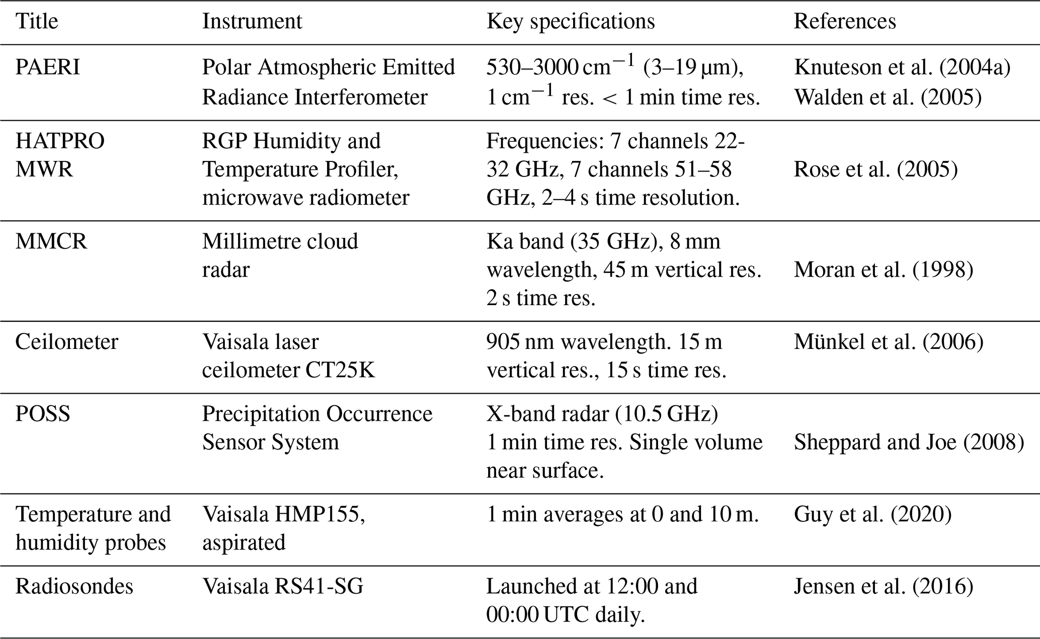
We use the tower-mounted temperature probes (Vaisala HMP155, installed in aspirated shields) as “true” reference points to assess the performance of the surface temperature retrievals from the MWR and AERI. The instrument uncertainty for the HMP155 is $<\pm \mathrm{0.3}$ ^∘C. For this study, we define the “surface” as the height of the raised platform photographed in Fig. 1, where both the AERI and MWR windows are situated. This surface is aligned with the HMP155 sensor mounted on the tower at 4 m above the snow surface; measurements from this sensor are henceforth referred to as surface temperature. Measurements from the HMP155 sensor located 10 m higher on the tower are compared to the 10 m thermodynamic retrievals. The same height adjustment is applied to the radiosonde profiles prior to comparison (which are launched approximately 3 m below the platform “surface” or 1 m above the snow surface). The uncertainty in the radiosonde measurements is ±4 % relative humidity and ±0.3 ^∘C (Jensen et al., 2016).

2.1.1 The AERI

The polar AERI (PAERI) at Summit was designed and manufactured by personnel at the Space Science and Engineering Center (SSEC) at the University of Wisconsin-Madison and is one of the original AERIs developed for the US Department of Energy's Atmospheric Radiation Measurement (ARM) program (Turner et al., 2016). It was built and calibrated according to specifications in Knuteson et al. (2004a) and adheres to the performance requirements of radiometric calibration (<1 %, 3σ, of ambient radiance) and spectral calibration (1.5 ppm, 1σ), as explained by Knuteson et al. (2004b). The PAERI measures downwelling spectral infrared radiance between 3 and 19 µm at an unapodized spectral resolution of about 0.48 cm⁻¹ (see Table 3 from Knuteson et al., 2004a). The PAERI operates on a continuous measurement schedule where it obtains views of the hot and ambient calibration sources followed by eight consecutive views of the sky at zenith. The sequence is repeated so that each set of eight sky views is bracketed in time by views of both calibration sources; these sources are then used to calibrate the eight sky views. Each of the spectral measurements is a “co-addition” of six interferometric scans. Each complete, calibrated measurement sequence takes approximately 3 min with the sky views separated by approximately 15–20 s. This yields more than 3300 infrared spectra each day. Quality control is then applied to each of the spectra by eliminating those that have instrument parameters outside of acceptable limits; the acceptable limits were set by SSEC personnel. The important instrument parameters are the responsivities and noise-equivalent radiances of the hot blackbody calibration source measured by both of the PAERI detectors (InSb and MCT) plus the electric current and temperature of the Stirling cooler that maintains the detectors at 77 K. In actuality, the instrument responsivities are a very sensitive indicator of the PAERI's health, and most unusable spectra are eliminated by low responsivity associated with small amounts of snow on the PAERI scene mirror. Finally, the remaining calibrated sky views are subjected to noise filtering using the technique described by Antonelli et al. (2004) and Turner et al. (2006).

2.1.2 The MWR

The MWR at Summit, a Humidity and Temperature Profiler (HATPRO) from Radiometer Physics GmbH, observed downwelling radiation in all 14 channels simultaneously every 4 s (see Table 2 for channel details). After collecting 600 zenith views, the HATPRO collected elevation scans at 5.4, 10.2, 16.2, 19.2, 23.4, 30.0, and 42.0 on either side of zenith. These elevation scans were used to both evaluate and update the calibration accuracy of the K-band channels (i.e. the low opacity channels between 22 and 32 GHz) using the tip-curve technique (Han, 2000). The more opaque V-band channels (i.e. in the 51–58 GHz band) were calibrated twice yearly using an external liquid nitrogen target; the most recent calibration used for this analysis was performed on 1 May 2019. Both the tip curves and the liquid nitrogen views are used to determine the effective temperature of the internal noise diode, which is used regularly when viewing the internal blackbody to establish two different reference values (i.e. one ambient blackbody view with the noise diode off and one “hot” blackbody view with the noise diode on). These internal blackbody views, which are done every minute, are used to continually update the gain of the radiometer and convert the observed signal to brightness temperature (T_b) following the calibration principles outlined in Liljegren (2000).

However, since the liquid nitrogen calibrations are performed infrequently, any drift in the effective temperature of the noise diode in the V-band channels will result in a calibration bias. Using a radiative transfer model (the monochromatic MonoRTM, Clough et al., 2005) with radiosonde profiles as input, we have determined a T_b offset that is subtracted from the observed brightness temperatures. The bias correction and the impact of not applying this correction prior to performing the thermodynamic retrievals are discussed in Appendix A.

Table 2 Centre frequencies, assumed noise level, whether the elevation scans for the frequency are included in the observation vector, and the bias offset applied to the observations for the HATPRO MWR at Summit.

2.2 Case study identification

For forecasting and nowcasting purposes, fog is usually defined by a threshold in horizontal visibility (typically <1000 m), which has important implications from a safety perspective (Gultepe et al., 2007). However, limiting the definition of fogs to those that reduce visibility to <1000 m encourages thinner fogs (or mists) to be ignored or incorrectly classified as clear-sky events. Being able to accurately measure thinner fogs is extremely important because (a) they form the precursor to thick fog, (b) they modify the surface moisture, aerosol, temperature, and radiative structure that might impact fog development further down the line (Haeffelin et al., 2013), and (c) they can have important radiative and climatological impacts even without developing into a thick fog (Cox et al., 2019; Hachfeld and Jürgens, 2000). Because both the MWR and AERI are directly sensitive to the radiative impact of fog (as opposed to visibility), for the purpose of this study, we define fog as the presence of near-surface liquid water that has a detectable radiative impact. Radiation fogs typically form under clear skies; as such, we only consider cases of fog under otherwise clear skies, which allows us to be certain that the LWP retrievals are a measure of fog LWP alone. The applicability of the results of this study to other types of fog is discussed in Sect. 4.

To identify case studies of radiation fog under otherwise clear skies, we only considered times when there were no clouds detected by the MMCR, which has a lowest range gate close to 200 m a.g.l. and is therefore insensitive to fog, and when there was no precipitation detected by the POSS, which is particularly sensitive to ice crystals. Of the times that these criteria were met, fog was provisionally identified when the 962 cm⁻¹ downwelling radiance measured by the AERI was greater than a threshold of 1.7 RU (radiance units, 1 RU = 1 mW m⁻² sr⁻¹ cm⁻¹). In the extremely dry atmosphere over Summit, the 962 cm⁻¹ microwindow is almost completely transparent under clear skies and is therefore particularly sensitive to the presence of clouds (e.g. Cox et al., 2012). The threshold value of 1.7 RU was 3 standard deviations above the mean 962 cm⁻¹ radiance during 179 verified clear-sky hours between June and September 2019 and therefore identified when the AERI window was obscured by cloud/fog with a detectable radiative impact. Ambiguous cases when there was evidence that something other than fog may have caused the 962 cm⁻¹ radiance increase, such as clear-sky ice crystal precipitation, high cirrus clouds, or the plume from the station generator, were removed based on the observer log and photographs. Table 3 details the 12 cases that met the criteria above and were selected for the intercomparison. In each case, the fog formed in late evening or early morning and usually dissipated by midday, as is characteristic of radiation fog (Fig. 2). Note that for 11 of these cases, there was no cloud base height detected by the ceilometer during the event, indicating that the events were indeed fog as opposed to low cloud. The only exception is for case ID 11, during which the ceilometer detected a cloud base between 52 and 105 m intermittently between periods of obscured vertical visibility.

Table 3 Details of the 12 radiation fog cases used in this study, including mean temperatures (T) and water vapour mixing ratios (wv). Note that the minimum visibility comes from observer reports at 00:00, 12:00, and 18:00 UTC and may not represent the minimum visibility outside of these times. Values where data were not available are indicated by NA – for example, when the observer did not log a visibility within the fog time frame or when the ceilometer did not report an obscured vertical visibility. Local time is UTC−3 h.

Figure 2 Diurnal distribution of fog during the summer 2019 case studies listed in Table 3 (blue bars). Black dashed lines show the maximum and minimum solar elevation angles (June–September 2019). Local time at Summit is UTC−3 h.

2.3 Retrieval methodology

We retrieve boundary layer thermodynamic profiles (temperature, T, and water vapour mixing ratio, wv) and LWP at a 5 min temporal resolution using the TROPoe iterative optimal estimation physical retrieval algorithm that is detailed in Turner and Lohnert (2021) and Turner and Blumberg (2019). TROPoe uses a forward model to calculate the observation vector from the current state vector, where the state vector is the retrieved thermodynamic profile and LWP, and the observation vector is the downwelling radiance observed by either the polar AERI or HATPRO MWR. Note that the observation vector from the MWR includes data from the elevation scans at 10.2, 16.2, and 19.2 degrees for the four most opaque V-band channels; including elevation scans in the retrieval has been shown to increase the accuracy of the retrieved temperature profile (Crewell and Lohnert, 2007). The forward models are line-by-line radiative transfer models; the LBLRTM version 12.1 (Clough and Iacono, 1995) simulates the AERI spectral radiances, and the monochromatic MonoRTM (Clough et al., 2005) simulates the MWR radiances. Note that the latter uses the improved temperature-dependent liquid water absorption coefficients (Turner et al., 2016). The state vector is incrementally adjusted to minimise the difference between the forward model calculation and the observation vector until the change between successive iterations is less than the uncertainty in the current state vector (Rodgers, 2000).

Due to the limited vertical resolution of the MWR, operational retrievals of thermodynamic profiles from MWRs are typically also constrained by an in-situ measurement of surface temperature, usually from a sensor that is integrated with the MWR (e.g. Cimini et al., 2015). For this study, we run TROPoe in three physically consistent configurations: once using only the PAERI radiances as the observation vector (as in Turner and Löhnert, 2014, henceforth named AERIoe), once using only the microwave brightness temperature observations from the HATPRO MWR (as in Löhnert et al., 2009) to provide a direct comparison of the relative sensitivity of the two instruments (henceforth named MWRoe), and lastly using the same configuration as the MWRoe but this time being additionally constrained by the in-situ surface temperature and water vapour observations from the HMP155, as it would be in an operational setting (henceforth named MWRoe-sfc).

Thermodynamic retrieval from passive spectral radiance observations is an ill-posed problem; hence the optimal-estimation retrieval is necessarily constrained by an a priori probability density function (the prior) that provides the first guess state vector that stabilises the retrieval (Turner and Löhnert, 2014). Typically, a location-specific prior can be derived from a database of historical observations (i.e. from radiosonde profiles) at or near the location of interest. The prior for Summit is computed from 1756 summer radiosonde launches (2010–2018). However, due to the rapid warming in the Arctic (e.g. Koenigk et al., 2020), this does not encapsulate the exceptionally warm and moist conditions at Summit during the summer of 2019 (NSIDC, 2019). To allow the retrievals more flexibility to account for the exceptional conditions, we have re-centred the prior using the mean of the three radiosondes closest to the retrieval date (whilst conserving relative humidity) and increased the wv variance in the prior by a factor of 4 at the surface (decreasing to 0 by 1 km a.g.l.).

Previous studies have used cloud base height (CBH) derived from a collocated ceilometer as an additional constraint on the retrieval, which allows the retrieval of below-cloud thermodynamic profiles from the AERI in the presence of thick clouds (Turner et al., 2007; Turner and Löhnert, 2014; Blumberg et al., 2015). Because we focus on radiation fogs under otherwise clear skies – which are, by definition, based at the surface – we initially assumed that the CBH is 5 m a.g.l. in all cases. However, large temperature biases (>5 K) in the AERIoe retrievals during fog illustrated that the TROPoe is highly sensitive to the CBH assumption when using AERI data as an input (see Sect. 3.1). For the final retrievals, we used CBH from the ceilometer to constrain the retrieval if the ceilometer detected a cloud base within 10 min of the retrieval time; if the ceilometer reported obscured vertical visibility, then the detected vertical visibility height (Morris, 2016) was input as the CBH. If neither of these situations occurred, the CBH assumption defaulted to 5 m a.g.l. The sensitivity of the retrievals to this choice is discussed further in Sect. 3.1. We ran all retrievals for up to 3 h before and after each fog event to encapsulate the atmospheric conditions on either side of radiation fog formation. The retrieval algorithm outputs 1σ uncertainties for all variables that incorporate the random error from the observations, the correlated error propagated from the prior, and the sensitivity of the forward model. Errors related to the CBH assumption or phase assumption (when only liquid water is considered) are not included, and we discuss these below in Sects. 3.1 and 4.

2.4 Evaluation metrics

To evaluate the three TROPoe retrieval configurations (AERIoe, MWRoe, and MWRoe-sfc), we focus on three aspects that are crucial for making accurate fog forecasts with NWP models, for visibility nowcasting, and for understanding the climatic impact of fog:

1. accurate representation of the structure of the temperature and humidity profile in the lowest 1 km a.g.l.

2. detection of the presence and strength of shallow surface-based temperature inversions that typically portend the formation of radiation fog

3. detection of the initial increase in LWP that signifies the onset of fog and a reduction in horizontal visibility.

To evaluate the accuracy of the temperature and humidity profile retrievals in the lowest 1 km a.g.l., we assess the performance of the MWRoe-sfc and AERIoe against 14 coincident radiosonde profiles by evaluating the mean bias and spread between the radiosonde profiles (truth) and the retrievals. We use modified Taylor diagrams (Taylor, 2001; Turner and Löhnert, 2014) to assess how well the retrieved profiles capture the shape of the true profiles by considering the Pearson's correlation coefficient and the ratio of the standard deviation of the retrieval to that of the truth profile. These results allow for a direct comparison with Blumberg et al. (2015), who compare TROPoe retrievals based on MWR and AERI observations to a larger number of radiosonde profiles (127) in southwestern Germany (but only consider clear-sky days or clouds with bases >500 m a.g.l.).

To evaluate the ability of each retrieval to detect the occurrence and strength of surface-based temperature inversions, we compare the retrieved surface (0 m) and 10 m temperatures with measurements from in-situ temperature sensors (see Sect. 2.1). We define the inversion “strength” as the 10–0 m temperature and evaluate the Pearson's correlation coefficients and root-mean-squared error (RMSE) between the retrieved values and the “truth” (the in-situ temperature sensors). Although we are limited by a maximum sensor height on the tower, we expect the 10–0 m temperature difference to be a good indicator of whether or not the retrieval captures the surface-based temperature inversion, since most of the inversion during radiation fog often occurs in the lowest 10 m a.g.l. (Price, 2011; Izett et al., 2019). We also compare the retrieved inversion strength over a deeper layer (100–10 m) with the 14 coincident radiosonde profiles.

Finally, in the absence of an independent method of determining LWP, we evaluate the ability of each retrieval to detect the initial increase in LWP, which is defined in this study as an indicator of fog formation that might lead to visibility reduction, with “fog onset” being defined as the point at which the retrieved LWP minus 2σ uncertainty (which is directly computed by TROPoe) increases above 0.1 g m⁻² for at least 10 min. We then compare the difference in fog onset detection time between the MWRoe and the AERIoe for each case study. We use the ceilometer range-corrected attenuated backscatter as an independent indicator of fog onset time. This methodology allows us to compare the sensitivity of the two sets of retrievals to small increases in liquid water that can begin to reduce visibility and impact radiative energy fluxes at the surface.

3 Results

3.1 Retrieval performance and sensitivity to cloud base height assumption

All 2045 retrievals from each configuration of TROPoe converged, meaning that the retrieval algorithm was able to find a solution within the maximum number of iterations. The mean RMSE between the final forward model calculation and the observed PAERI radiance across all AERIoe retrievals was 0.54±0.09 RU, which is of the order of the instrument noise level (Blumberg et al., 2015). For the MWRoe retrievals the mean RMSE between the final forward model calculation and the MWR brightness temperatures was 0.38±0.12 K, again within the instrument noise level (Rose et al., 2005). The MWRoe and MWRoe-sfc are comparable in terms of RMSE, liquid water path retrieval and thermodynamic profile retrievals above 100 m a.g.l., so we only discuss the difference between the MWRoe and MWRoe-sfc when we consider the ability of each retrieval configuration to capture the strong surface-based temperature inversions associated with radiation fog in Sect. 3.3.

The AERIoe retrievals were very sensitive to the cloud base height (CBH) assumption. Because we are only considering cases of radiation fog under otherwise clear skies, the first iteration of retrievals assumed that, if liquid water was detected, the cloud base height was 5 m a.g.l., removing the requirement for additional instrumentation to detect CBH. Figure 3a demonstrates that, under this assumption, the AERIoe retrieved unrealistic temperature profiles in some cases when the fog was optically thick (i.e. ceilometer is obscured) or when the ceilometer detected a cloud with a base close to 1300 m a.g.l. prior to the start of the fog event. The unrealistic temperature profiles manifest as exceptionally warm temperatures just above the surface, indicated by red colours in Fig. 3.

Previous AERIoe algorithms have used the ceilometer “first cloud base height field” (an output of the Vaisala proprietary software) to estimate CBH (Turner and Löhnert, 2014; Blumberg et al., 2015). Using this assumption rather than simply assuming the CBH to be 5 m a.g.l. reduced the temperature profile artefacts in some but not all cases (Fig. 3b). The ceilometer software also outputs a vertical visibility field (described in Morris, 2016) when the extinction profile is such that the atmosphere is obscured but no distinct cloud base can be determined, as often happens in the case of thick fog. The remaining artefacts in the example case study occur when the ceilometer reports a vertical visibility value (Fig. 3b). When we used the vertical visibility field in addition to the first cloud base height field to provide the CBH assumption in the AERIoe retrieval, the remaining artefacts were removed (Fig. 3c).

Figure 3 Temperature profiles during the 5 September case study from three iterations of the AERIoe retrieval using different CBH assumptions. The ceilometer first cloud base height field is overlaid as cyan crosses, and the vertical visibility field is overlaid as black circles. (a) Assumed CBH was 5 m a.g.l. any time LWP>0; (b) assumed CBH was set to the ceilometer first cloud base height if the ceilometer detected a cloud within the 10 min centred on the retrieval time, otherwise 5 m a.g.l.; (c) as in (b) except if the ceilometer reported “obscured” the CBH was set equal to the ceilometer maximum vertical visibility field.

Even if the fog is reducing visibility at the surface, the cloud base height is the height at which the fog becomes optically thick to the PAERI, which is similar to when it becomes optically thick for the ceilometer (which uses radiation in the near-infrared, 905 nm). Figure 3 shows that a difference in CBH of just 30 m can make a significant difference to the retrieval when the cloud is close to the surface, demonstrating that accurate CBH measurements are a necessary input to the AERIoe for retrieving thermodynamic profiles in the presence of fog or near-surface clouds. In contrast, the MWRoe was not sensitive to the CBH assumption, because clouds are markedly more transparent at microwave frequencies. For the remainder of this study, all retrieval configurations derive CBH from both the first cloud base height and the vertical visibility field of the ceilometer.

3.2 Performance of retrieved thermodynamic profiles in the lowest 1 km a.g.l.

The AERIoe temperature profiles (0–1 km a.g.l.) compared extremely well to the 14 radiosonde profiles considered, with a mean bias of −0.43 ^∘C and a mean RMSE of 1.0 ^∘C (Fig. 4a). The MWRoe temperature profiles exhibited a vertically consistent negative bias compared to the radiosonde profiles, with an average value of −1.5 ^∘C and an average RMSE of 1.7 ^∘C (Fig. 4a). Although investigating the source of the negative bias in the MWRoe temperature profile is outside the scope of this study, such systematic biases can often be corrected for, and the similar spread in bias magnitude between the AERIoe and the MWRoe temperature retrievals imply that the performance of the two sets of retrievals would be similar after an additional bias correction (Fig. 4a). For both sets of retrievals, the temperature RMSE is largest in the lowest 50 m a.g.l., where it approaches 2.0 ^∘C (Fig. 4a); this is also the case for the MWRoe-sfc, which looks qualitatively similar (not shown).

For water vapour, the performance of the AERIoe and MWRoe retrievals compared to the radiosonde profiles was very similar (Fig. 4b). Neither set of retrievals exhibited a mean bias, and the RMSE of the AERIoe retrievals was slightly smaller than the MWRoe up to 800 m a.g.l., with a mean value of 0.39 g kg⁻¹ (compared to 0.44 g kg⁻¹ for the MWRoe).

Figure 4c and d show that both sets of temperature profile retrievals are better correlated with the radiosonde profiles (r>0.98, Fig. 4c,) than the water vapour profile retrievals, which in some cases have correlation coefficients <0.7 (Fig. 4d), and the spread in the standard deviation ratio is much smaller for the temperature retrievals (0.9–1.2) than for the water vapour profile retrievals (0.6–1.3). The AERIoe retrievals (for both temperature and water vapour) have a similar spread in correlation coefficients and standard deviation ratios than the MWRoe retrievals, indicating that the performance of the two retrievals was comparable across this subset of profiles.

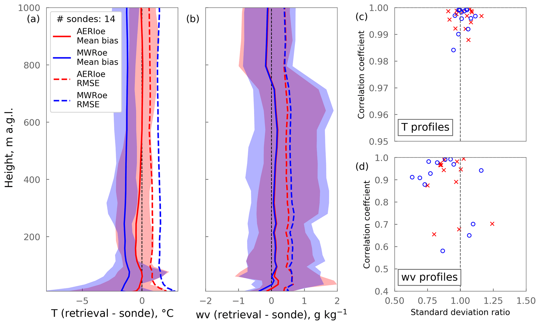
Figure 4 Comparison between retrieved thermodynamic profiles and the 14 coincident radiosonde profiles in the lowest 1 km a.g.l. (a) The temperature and (b) and water vapour bias (retrieval – radiosonde) for AERIoe retrievals (red) and MWRoe retrievals (blue); the solid line shows the mean bias and the shaded represents the range. Dashed lines show the root-mean-squared error (RMSE). (c) The temperature and (d) water-vapour-modified Taylor plots showing the relationship between the correlation coefficient and standard deviation ratio for each retrieval/radiosonde pair ([1,1] represents a perfect score) for the AERIoe retrievals (red) and the MWRoe retrievals (blue).

3.3 Characterisation of shallow surface-based inversions

The AERIoe temperature retrievals at 0 and 10 m a.g.l. are equally well correlated with observations (r=0.99, RMSE=1.1 ^∘C), indicating that the AERIoe captures vertical temperature gradients in the lowest 10 m of the atmosphere well and retrieves surface temperatures with consistently high accuracy (Fig. 5). In comparison, the MWRoe retrievals perform worse than the AERIoe at both heights, with r=0.86, RMSE=4.2 ^∘C at 0 m, and r=0.95, RMSE=2.1 ^∘C at 10 m (Fig. 5). Notably, the performance of the MWRoe is worst at 0 m, where the MWRoe typically has a warm bias at colder temperatures (72 % of the time when $T<-\mathrm{7}$ ^∘C) and a cold bias at warmer temperatures (93 % of the time when $T>-\mathrm{7}$ ^∘C). This bias reduced at 10 m, implying that the temperature lapse rate between 0 and 10 m a.g.l. is often incorrect in the MWRoe retrieval (Fig. 5).

For the MWRoe-sfc, which includes the surface temperature as an additional constraint in the retrieval, the correlation with in-situ surface temperature measurement is perfect, suggesting that very little additional variability is introduced by the microwave radiance measurements. Despite this, the 10 m temperature retrievals from the MWRoe-sfc perform only marginally better than those of the MWRoe compared to the in-situ measurements and not as well as the AERIoe, which did not have the advantage of the extra information from the in-situ surface temperature probe (Fig. 5). This suggests that constraining the retrieval by the in-situ surface temperature does not translate to improvements in the temperature profile retrieval above that level.

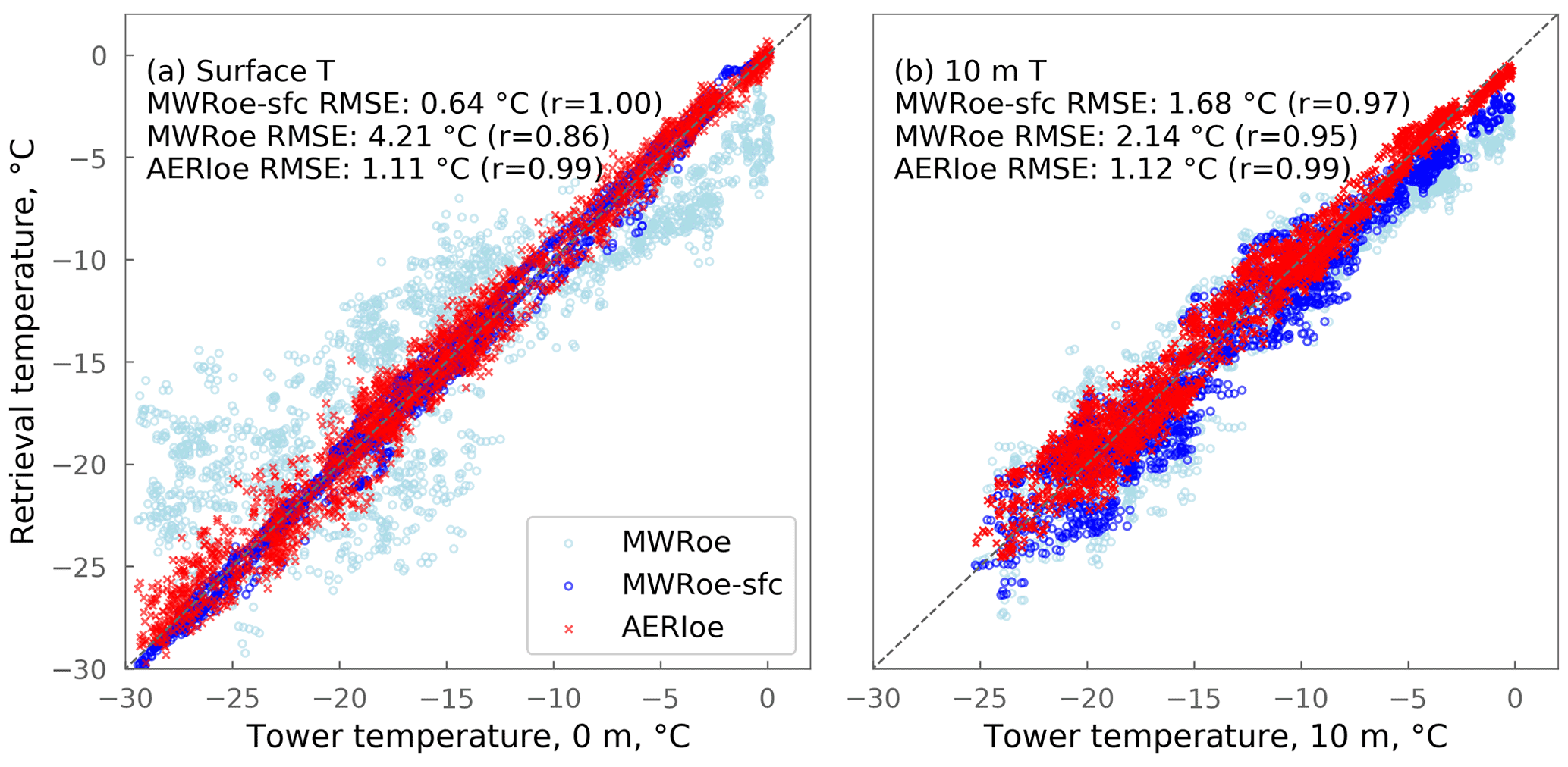
Figure 5 Retrieved temperature versus in-situ measurements from the tower at the surface (a) and 10 m (b). The MWRoe retrievals are plotted as pale blue circles, the AERIoe retrievals as red crosses, and the MWRoe retrievals that are constrained by the surface temperature (MWRoe-sfc) are dark blue circles. The Pearson's correlation coefficient (r) and root-mean-squared error (RMSE) between each set of retrievals and the tower measurements are included on the figure. All correlations are significant at the 99 % confidence level. The dashed grey line represents perfect agreement.

Figure 6a confirms that the MWRoe is not able to capture the 0–10 m temperature lapse rate by demonstrating that there is no correlation between the measured surface-inversion strength (10–0 m T) and that retrieved by the MWRoe. In fact, the 10–0 m lapse rate is essentially constant in the MWRoe, implying that retrieved temperatures at 0 and 10 m are highly correlated. In contrast, the AERIoe surface-inversion strength is well correlated with in-situ measurements (r=0.80) with an RMSE of 1.9 ^∘C (Fig. 6a), demonstrating that the AERIoe can accurately retrieve shallow surface temperature inversions with lapse rates of up to −1.2 ^∘C m⁻¹. When the in-situ surface temperatures are used to constrain the MWR retrieval (in the MWRoe-sfc), the ability of the retrieval to capture the shallow temperature inversions is considerably improved (Fig. 6a). Note that the correlation between the MWRoe-sfc near-surface temperature inversion and the in-situ measurements in Fig. 6a is not a fair assessment of performance, since the retrieval results are not independent from the in-situ measurements. Nonetheless, it highlights the importance of using accurate surface temperature measurements to constrain MWR temperature retrievals.

The radiosonde profiles provide an alternative independent measure of surface-inversion strength, allowing the comparison of the ability of each retrieval configuration to capture surface temperature inversions over a deeper layer. Figure 6b compares the 100–10 m retrieved inversion strength with that measured by the 14 coincident radiosonde profiles. Over this depth, the RMSE of the AERIoe and the MWRoe-sfc are comparable to the values for the 10–0 m comparison (1.65 and 1.83 ^∘C m⁻¹ respectively), but the MWRoe RMSE remains much larger (2.22 ^∘C m⁻¹), demonstrating that the MWRoe alone is not capable of accurate retrievals of surface temperature inversions even in this deeper layer. Only the AERIoe retrievals in this case are significantly correlated (r=0.46) with the radiosonde measurements, although the small number of radiosondes available for comparison makes it difficult to draw robust conclusions from this result. Klein et al. (2015) compared AERI-derived lapse rate 100–10 m against more than 200 radiosondes in Oklahoma (southern US) and found very good agreement with r² values >0.93.

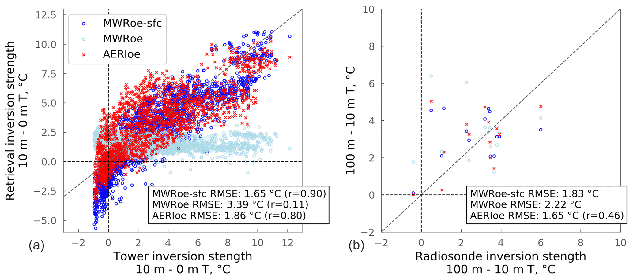
Figure 6 (a) Inversion strength (10–0 m temperature, T) retrieved from the AERIoe (red), the MWRoe (light blue), and the MWRoe-sfc (dark blue) versus observations from the tower-mounted HMP155 probes. (b) The same as (a) except for the 100–10 m inversion strength compared to observations from 14 coincident radiosonde profiles. On both subplots, the diagonal grey dashed line represents perfect agreement, and the horizontal and vertical dashed black lines at 0 ^∘C delineate when a surface-based temperature inversion is present (right quadrants) versus absent (left quadrants). The root-mean-squared error (RMSE) values are included on the plots, and the Pearson's correlation coefficients (r) are only included when they are significant at the 90 % confidence level.

The reason that the AERIoe can accurately retrieve shallow surface-based temperature inversions but the MWRoe cannot is because the AERI infrared radiance measurements theoretically contain much more information about the near-surface temperature profile than the MWR brightness temperatures (Blumberg et al., 2015). Figure 7 supports this by illustrating that the degrees of freedom for signal for temperature from the AERIoe retrievals is greater than that from the MWRoe retrievals, especially at the surface. The degrees of freedom for signal is a measure of the number of independent pieces of information from the observation vector that the retrieval used to generate the solution (Rodgers, 2000). Figure 7 shows that the AERIoe has around 6 times as much information about the surface temperature than the MWRoe and twice as much at 10 m. The mean degrees of freedom for signal for the surface temperature retrieval is over 4 times higher for the MWRoe-sfc compared to the MWRoe due to the additional information about the surface temperature in the observation vector. However, above the surface, the AERIoe still contains more information about the temperature profile than the MWRoe-sfc in the lowest 500 m of the boundary layer, the region in which accurate temperature profiles in NWP models are critical for successful fog forecasts (Martinet et al., 2020).

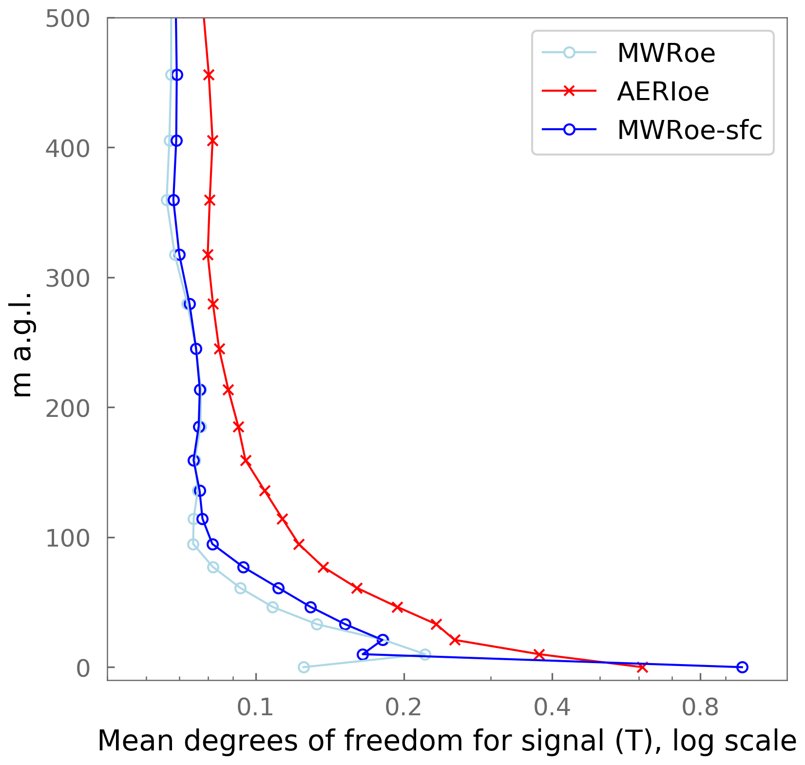
Figure 7 Mean degrees of freedom for signal across all temperature retrievals from the MWRoe (pale blue), the AERIoe (red), and the MWRoe constrained by the in-situ surface temperature measurement, MWRoe-sfc (dark blue).

3.4 LWP retrievals and the detection of fog onset

The LWP retrievals from the AERIoe and MWRoe were well correlated (r=0.88) and fell within ±5 g m⁻² of each other in ∼90 % of all retrievals; however, on occasion, there were discrepancies of up to 10 g m⁻² (Fig. 8), which can be equivalent to significant differences in horizontal visibility and net surface radiative forcing (see example in Sect. 1).

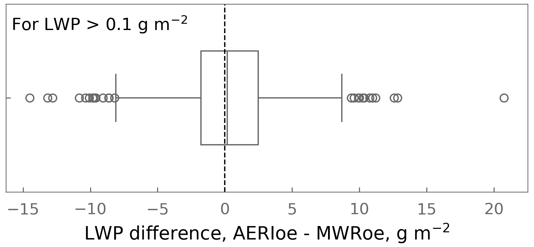
Figure 8 The differences in retrieved liquid water path (LWP) between all AERIoe and the MWRoe retrievals (LWP>0.1 g m⁻²). A total of 50 % of all retrievals fall within the central box, 90% of all retrievals fall within the box plot “whiskers”, and the remaining data are plotted as outliers (circles).

Although we do not have an independent measure of the “true” LWP, Fig. 9 illustrates the difference in the sensitivity of the MWRoe and the AERIoe to LWP as a function of LWP magnitude. The PAERI radiance observations are very sensitive to changes in LWP when the LWP is small, and so the 1σ uncertainty in the retrieved LWP from the AERIoe is less than 1 g m⁻² for LWP<20 g m⁻² (or less than 10 %, Fig. 9). In contrast, the uncertainties in LWP derived from MWR brightness temperatures are related to absolute radiometric uncertainties that are approximately constant with respect to LWP, equating to at least 50 % uncertainty for LWP<10 g m⁻² (Fig. 9). However, as the LWP approaches opacity in the infrared (>40 g m⁻²), the sensitivity of the PAERI radiance observations to changes in LWP decreases until the uncertainties in the LWP retrievals from the AERIoe become equivalent to those from the MWRoe (∼3 g m⁻² or ∼6 % uncertainty at 50 g m⁻²).

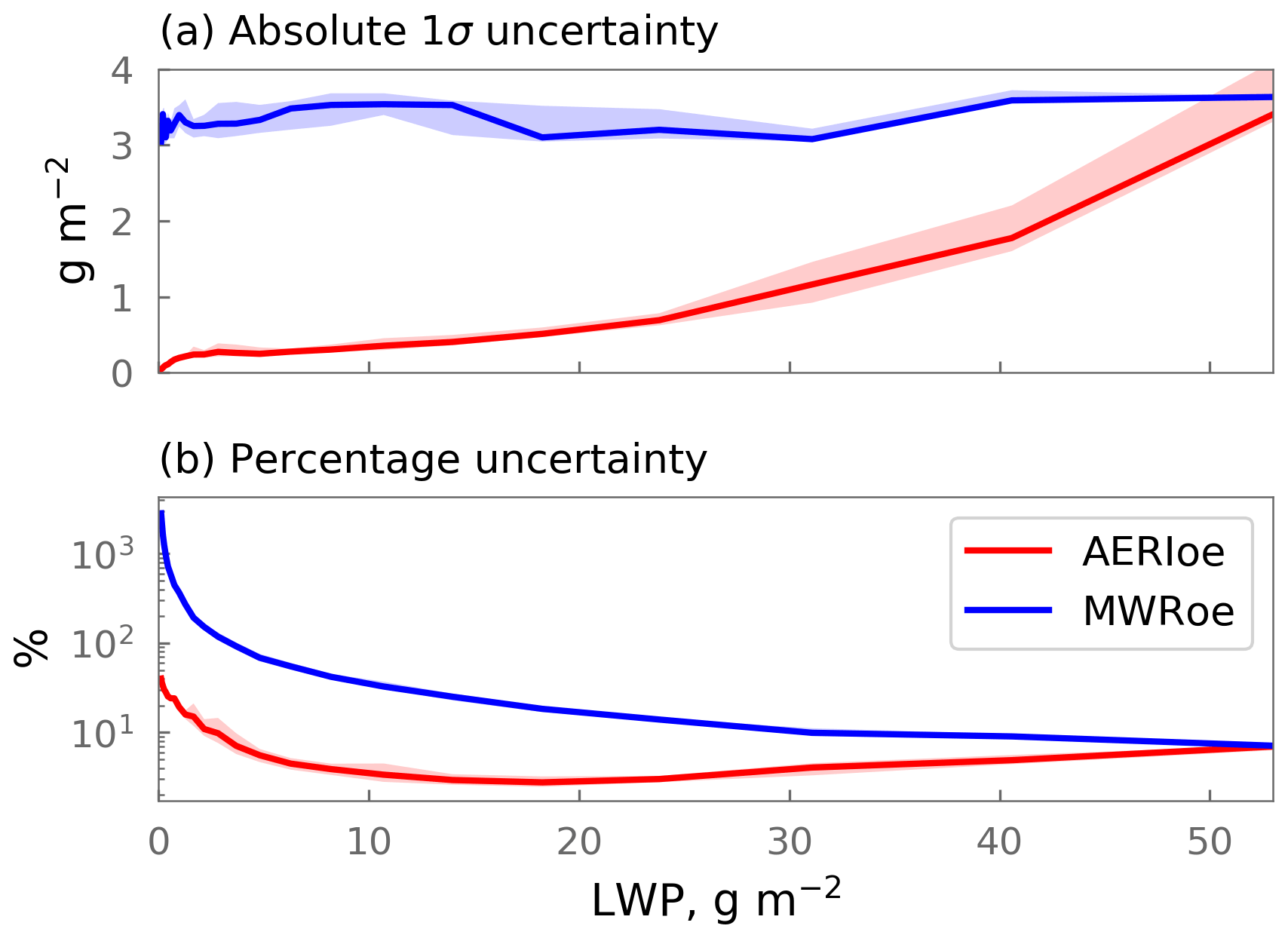
Figure 9 1σ uncertainty in the AERIoe (red) and MWRoe (blue) liquid water path (LWP) retrievals as a function of LWP. (a) Shows the absolute uncertainties, and (b) shows the percentage uncertainties. The solid line is the median of all retrievals and shading is the interquartile range.

The high sensitivity of the AERIoe to changes in LWP when LWP is small means that the increase in LWP associated with the development of radiation fog under clear skies is detected earlier in the AERIoe retrievals compared to the MWRoe retrievals (following our fog definition as the presence of near-surface liquid water that has a detectable radiative impact). The increased sensitivity of the infrared over the microwave to small LWP values was described in (Turner, 2007). This is illustrated in Fig. 10, which shows the development of LWP during the 15 July 2019 case study. Shortly after 23 h on 15 July, the AERIoe detected a significant LWP that continued to increase gradually at a rate of ∼1.4 g m⁻² h⁻¹, until 02:00 h on 16 July, after which it increased rapidly to ∼30 g m⁻² at 03:00 h (Fig. 10). In contrast, due to the larger uncertainties in the MWRoe LWP retrieval, the MWRoe LWP did not increase to a value that was significantly different from the noise until the onset of the rapid LWP increase just after 02:00 h.

For independent verification, we also determine fog onset from the ceilometer range-corrected attenuated backscatter. We define the ceilometer fog onset as being where the 5 min mean total backscatter increases by more than 3 standard deviations from the mean clear-sky backscatter at Summit between 1 June and 30 September 2019 (the mean clear-sky backscatter is determined using the same subset of verified clear-sky hours used to identify fog events from the AERI radiance, Sect. 2.2). Ceilometer attenuated backscatter is sensitive to the scattering cross section of molecules and particles in the atmosphere and can be sensitive to the presence of atmospheric aerosols (e.g. Markowicz et al., 2008) and to the hygroscopic growth of aerosols prior to their activation into fog droplets (Haeffelin et al., 2016), the latter of which can be a precursor to radiation fog formation (Haeffelin et al., 2016). At Summit, the aerosol scattering cross section is usually extremely small ($<\mathrm{2}\times {\mathrm{10}}^{-\mathrm{6}}$ m⁻¹ at 550 nm, Schmeisser et al., 2018), and any signal due to the presence of aerosols is incorporated into the calculation into the mean clear-sky backscatter. We do not distinguish between the detection of aerosol hygroscopic growth and droplet formation in the ceilometer backscatter.

For the 15 July 2019 case, the ceilometer detected fog onset shortly before 00:00 on 16 July, 40 min after the AERIoe (Fig. 10b). Despite the relatively low LWP, the visibility at 00:00 h was only 400 m, and the observer reported freezing fog, indicating that this signal was indeed due to the presence of liquid droplets. In this case, if the MWRoe LWP retrieval was used to detect fog or for visibility nowcasting, the fog at 00:00 h on 16 July would not have been detected, whereas if the AERIoe LWP retrieval was used instead, it would have been.

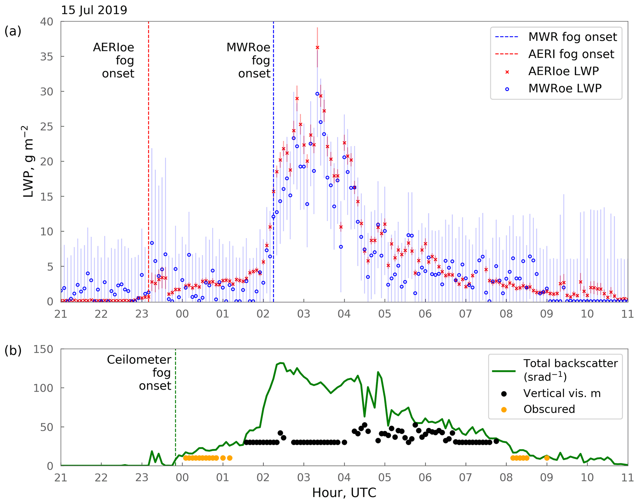
Figure 10 (a) The evolution of fog liquid water path (LWP) during the 15 July 2019 case study retrieved from the AERIoe (red) and the MWRoe (blue). Error bars show the 2σ uncertainty of the retrievals. The vertical red line shows the fog onset determined from the AERIoe retrievals, and the vertical blue line shows the fog onset determined by the MWRoe retrievals 3 h later. (b) Total range-corrected attenuated backscatter (5 min mean, green line) and vertical visibility (black points) from the ceilometer. Orange points indicate when the ceilometer reports obscured.

The ceilometer detects fog (or aerosol hygroscopic growth) for all cases, with the exception of case 7 (4 August). During this case, the fog was extremely thin (maximum LWP from the AERI only 2 g m⁻²), but the onsite observer logged the presence of a fog bow between 07:15 and 08:30, demonstrating that liquid water droplets were indeed present. This was a very marginal case that demonstrates the ability of the AERI to detect very small amounts of liquid water when even the ceilometer cannot. The MWRoe retrieval only detects fog for 6/12 cases (Fig. 11), and for those 6 cases, the AERIoe retrieval consistently detects the onset of fog (via the increase in LWP) before the MWRoe retrieval by 25 to 185 min (Fig. 11). For the 6 cases where the MWRoe does not detect the fog, the mean LWP detected by the AERIoe is very low (1.4 to 3.1 g m⁻²).

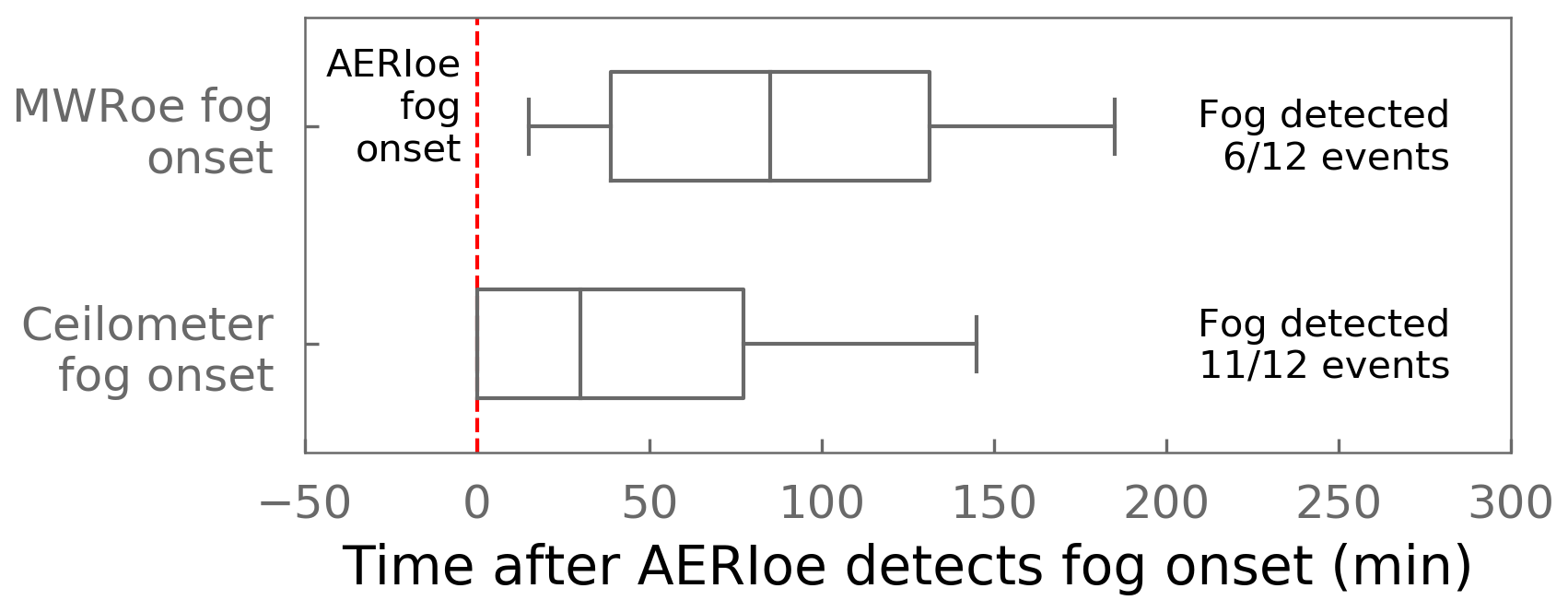
Figure 11 Time between fog onset detection from the AERIoe (vertical red line, t=0) and fog onset detection from the MWRoe (upper) and ceilometer (lower). Only cases where both methods detected fog are included (6/12 for the MWRoe and 11/12 for the ceilometer). The whiskers capture all data points; the box shows the interquartile range.

4 Discussion

Central Greenland provides an excellent opportunity to study climatologically relevant radiation fog due to the pristine environment, commonality of events, and presence of the ICECAPS's long-term, multi-instrument platform. Nonetheless, it is a unique environment, and therefore the applicability of the results of this study in other environments is not guaranteed. Comparing retrievals between locations is complicated by the dependence on the quality of different prior datasets and instrument calibrations. However, in general, the performance of the MWRoe and AERIoe thermodynamic profile retrievals in the lowest 1 km a.g.l. are comparable to the performance assessed in a similar way against 127 radiosonde profiles in southwestern Germany (Blumberg et al., 2015). Blumberg et al. (2015) found the mean RMSE in the temperature profiles (lowest 1 km a.g.l.) to be ∼0.9 ^∘C for the AERIoe and ∼1.1 ^∘C for the MWRoe (compared to 1.0 and 1.6 ^∘C in this study); for water vapour profiles, an RMSE of 0.7 g kg⁻¹ for the AERIoe and 1.0 g kg⁻¹ for the MWRoe was found (compared to 0.38 and 0.43 g kg⁻¹ in this study). Nevertheless, under certain conditions, we might expect the performance of the AERIoe to deteriorate. For example, in environments where the total column water vapour is very high (e.g. tropical regions), the atmosphere will have a higher opacity in the infrared and the AERI sensitivity will be reduced (Löhnert et al., 2009). Additionally, the high sensitivity of the AERI, which makes it so suited to the study of fog, also makes it sensitive to localised plumes of pollution or smoke and, in some cases, to atmospheric aerosols (e.g. Turner and Eloranta, 2008). Both sets of retrievals are also sensitive to the quality of the prior that is used to constrain the retrieval and provide a first guess (Turner and Löhnert, 2014) and to the calibration and characterisation of the particular instrument, which is typically more challenging for the MWR (see Appendix A, Blumberg et al., 2015, and Löhnert and Maier, 2012). All of these factors may impact performance at different locations and should be considered during experimental design. Note that neither instrument operates effectively in rain.

The radiation fog case studies presented in this study are all composed of supercooled water droplets, with some occurring at surface temperatures as low as −28 ^∘C (Table 3). Supercooled fogs at such cold temperatures are common at Summit, whereas ice fogs during the summer are rare (Cox et al., 2019). Observations of “fog bows” – atmospheric optics associated with the scattering of light by liquid water droplets – during most case studies confirm the presence of liquid water, as does the fact that the fogs are also detected by the ceilometer, which is not very sensitive to ice crystals (Van Tricht et al., 2014). However, the possibility exists that some (or even all) of these case studies contain ice crystals in addition to liquid water droplets. The scattering and absorption properties of ice crystals can be quite different to those of water droplets at wavelengths that are relevant for the AERIoe (e.g. Turner, 2005, Rowe et al., 2013), potentially resulting in biases in the AERIoe LWP retrievals that assume a liquid-only cloud. The lack of an independent “truth” value for LWP means that we cannot quantify any such biases. Nevertheless, the smaller uncertainties in the AERIoe LWP retrieval relative to the MWRoe LWP retrieval are related to the physical sensitivity of the measurement, and so we can expect this result to be consistent across other cases of warm fog.

This study focuses on cases of thin radiative fog (LWP<40 g m⁻²), which is the most common type of fog at Summit, and draws attention to the benefits of the AERI, which is particularly sensitive to the small changes in LWP and strong shallow temperature inversions that are characteristic of these events. For other types of fog, onset might not be initiated by a small increase in LWP; for example, in stratus-lowering events, the reduction in cloud base height from the ceilometer might be a better indicator of fog onset. At other locations (in the mid-latitudes, for example), thicker fogs with LWP>50 g m⁻² are more common and can be 100's of metres deep (Toledo et al., 2021). Although the AERI might still be a useful instrument for the early detection of such events, once the fog becomes optically thick in the infrared, the AERI can no longer provide information about the thermodynamic profile above the fog or the trend in LWP, both of which are useful parameters for understanding the development of deep well-mixed fog (Toledo et al., 2021). In such cases, thermodynamic profile and LWP retrievals from the MWR are valuable. The TROPoe algorithm can combine both AERI and MWR measurements in the same retrieval. Below-cloud thermodynamic profiles from the combined MWR+AERI are essentially the same as retrievals based on AERI measurements alone (Turner and Lohnert, 2021), but the uncertainty in the LWP retrieval when both instruments are combined is <20 % across the entire range in LWP from 1 to <500 g m⁻² (Turner, 2007).

Although this study focuses on the passive remote sensing instruments that are essential for fog detection (since the active remote sensing instruments have a blind spot immediately above the surface), complementary information from active remote sensing instruments are also necessary for accurate results. We demonstrate in Sect. 3.1 that accurate cloud base height detection (from the ceilometer) is an important input for the AERIoe retrievals, and the radar is also required to filter out precipitation events than can invalidate retrievals from both the MWR and the AERI. Overall, this study highlights the importance of instrument synergy to provide optimal thermodynamic profiles and LWP retrievals, supporting the findings of previous studies (Turner et al., 2007; Löhnert et al., 2009; Turner and Lohnert, 2021; Smith et al., 2021; Djalalova et al., 2022) and expanding on this conclusion to include the specific conditions pertaining to the development of radiation fog.

5 Summary and conclusions

Previous studies have demonstrated that AERI measurements of spectral infrared radiance are more sensitive to the structure of the near-surface temperature profile and to small changes in liquid water path (LWP) than MWR measurements of microwave brightness temperatures (Turner, 2007; Löhnert et al., 2009; Blumberg et al., 2015). The purpose of this study was to compare retrievals of boundary layer thermodynamic profiles and LWP from these two instrument types during cases of thin supercooled radiation fog in central Greenland using a consistent physical retrieval algorithm (the AERIoe retrieval based on observations of infrared radiance and the MWRoe based on microwave brightness temperatures). We assess the performance of the two retrievals against three criteria that are critically important for the forecast and detection of radiation fog:

1. ability to retrieve accurate thermodynamic profiles in the lowest 1 km a.g.l. of the atmosphere

2. ability to capture the strength and development of shallow surface-based temperature inversions that typically portend the formation of radiation fog

3. ability to detect the initial increase in LWP that signifies the onset of fog and a reduction in horizontal visibility.

Although there are only 14 coincident radiosonde profiles available for comparison, the bias and RMSE statistics of the temperature and water vapour profiles in the lowest 1 km a.g.l. are consistent with the findings of Löhnert et al. (2009) and Blumberg et al. (2015), suggesting that the performance of both sets of retrievals in the Arctic and under conditions for the formation of supercooled fog are similar to the performance in the mid-latitudes and under other sky conditions (clear skies or below clouds with bases above 500 m a.g.l.). We find that the water vapour profile retrievals in the lowest 1 km a.g.l. are comparable for both the MWRoe and the AERIoe, with RMSE of 0.44 g kg⁻¹ for the MWRoe and 0.39 g kg⁻¹ for the AERIoe. The AERIoe temperature profile retrievals perform better in terms of bias and RMSE than the MWRoe for the 14 cases considered (MWRoe bias: −1.5 ^∘C, RMSE: 1.7 ^∘C; AERIoe bias: −0.43 ^∘C, RMSE: 1.0 ^∘C); however, the consistency of the negative temperature bias in the MWRoe suggests that an additional bias correction may be possible, which would result in comparable performance between the two sets of retrievals.

A unique aspect of this study was the assessment of the ability of the two retrieval types to characterise shallow (0–10 m a.g.l.) surface-based temperature inversions. Despite the similar performance of the temperature profile retrievals up to 1 km a.g.l. in general, the ability of the two retrieval types to characterise the 0–10 m temperature lapse rate was markedly different. The AERIoe 0–10 m temperature differences were well correlated with in-situ observations, capturing surface temperature inversions well up to a lapse rate of −1.2 ^∘C m⁻¹ (previous studies have demonstrated the ability of the AERIoe to characterise near-surface lapse rates well for values of −0.01 to 0.01 ^∘C m⁻¹, Klein et al., 2015). However, the MWRoe 0–10 m temperature differences were not correlated with observations and did not deviate more than 1 ^∘C from the prior. The reason for this difference is that the infrared radiance measurements from the AERI contain more information about the temperature near the surface than the MWR measurements. This highlights the importance of using accurate surface temperature measurements to constrain MWR thermodynamic profile retrievals.

In addition to increased sensitivity to shallow surface temperature inversions, the AERI is much more sensitive to small changes in LWP, with the result that the uncertainties in retrieved LWP from the AERIoe are much smaller than those retrieved from the MWRoe for LWP<50 g m⁻². This means that the AERIoe is consistently able to detect small changes in LWP, which might initiate radiation fog and reduce horizontal visibility, by up to 185 min before the MWRoe. This has important implications for fog detection and visibility nowcasting, because even a very small LWP (<5 g m⁻²) can reduce horizontal visibility, and the MWRoe alone would not have detected fog on some occasions when reported visibility was as low as 400 m.

Based on these results, we hypothesise that the assimilation of near-surface temperature profile retrievals from an AERI into NWP models could improve fog forecasts beyond the improvements already seen through the assimilation of MWR measurements (Martinet et al., 2020). In addition, the increased sensitivity of the AERI to small changes in LWP (compared to the MWR) will allow the AERI to detect the onset of radiation fog events earlier, with the potential to increase the skill of fog nowcasting products and improve climatological analyses of fog radiative effects.

Although this study demonstrates that the AERI is particularly well suited to retrieving boundary layer properties that are key for radiation fog formation, there are trade-offs that must be considered when selecting instruments for operational use, notably that the AERI is unable to retrieve thermodynamic profiles above optically thick clouds/fog (LWP>40 g m⁻²), and that the AERIoe retrieval is particularly sensitive to the CBH assumption during fog/low cloud. This highlights the importance of a multi-instrument approach to improve fog forecasting under all sky conditions: ceilometer cloud base heights are necessary to generate accurate thermodynamic profile retrievals from the AERI; MWRs are needed to retrieve LWP and thermodynamic profiles above optically thick fog/clouds, and radar data is required to determine the presence of precipitation, which can invalidate retrievals from both passive instruments.

The results of this study present a case for future observing-system experiments (or observing-system simulation experiments, as in Otkin et al., 2011; Hartung et al., 2011) to quantify the impact of the operational use of AERI observations in terms of improvements to NWP skill, particularly in the case of radiation fog.

Appendix A: MWR T_b bias correction

An external liquid nitrogen target is used to determine the effective temperature of the MWR internal noise diode, which is required to convert the observed signal into brightness temperature (T_b) values, as described in Sect. 2.1.2. Due to the personnel and resource requirements, this calibration is only performed twice a year at Summit. Imperfect calibrations can result in a radiometric bias in the T_b measurements, and drift in the effective temperature of the internal noise diode can occur in between calibrations (Löhnert and Maier, 2012; Blumberg et al., 2015).

To determine this radiometric bias in the observed T_b values, the twice-daily radiosondes launched at Summit between 1 June and 31 August 2019 were used as input in the MonoRTM, and the bias between the observed and computed T_b values was determined. The evolution of the bias over time is well illustrated by showing the bias values for the cases used in this analysis (Fig. A1). The bias in the K-band channels remained very small (absolute value less than 0.5 K), confirming that the automated tip-curve calibration method applied to those transparent channels was working well. However, there is a significant negative bias (calculation larger than the observed radiance) in the 51 to 54 GHz channels, and this bias changes with time. However, the bias in the 51.26 and 52.28 GHz channels is variable with time with no apparent pattern (inset in Fig. A1). Fortunately, the T_b bias in the 55 to 58 GHz channels is stable with time, and the magnitude is relatively small (less than 0.7 K for those channels).

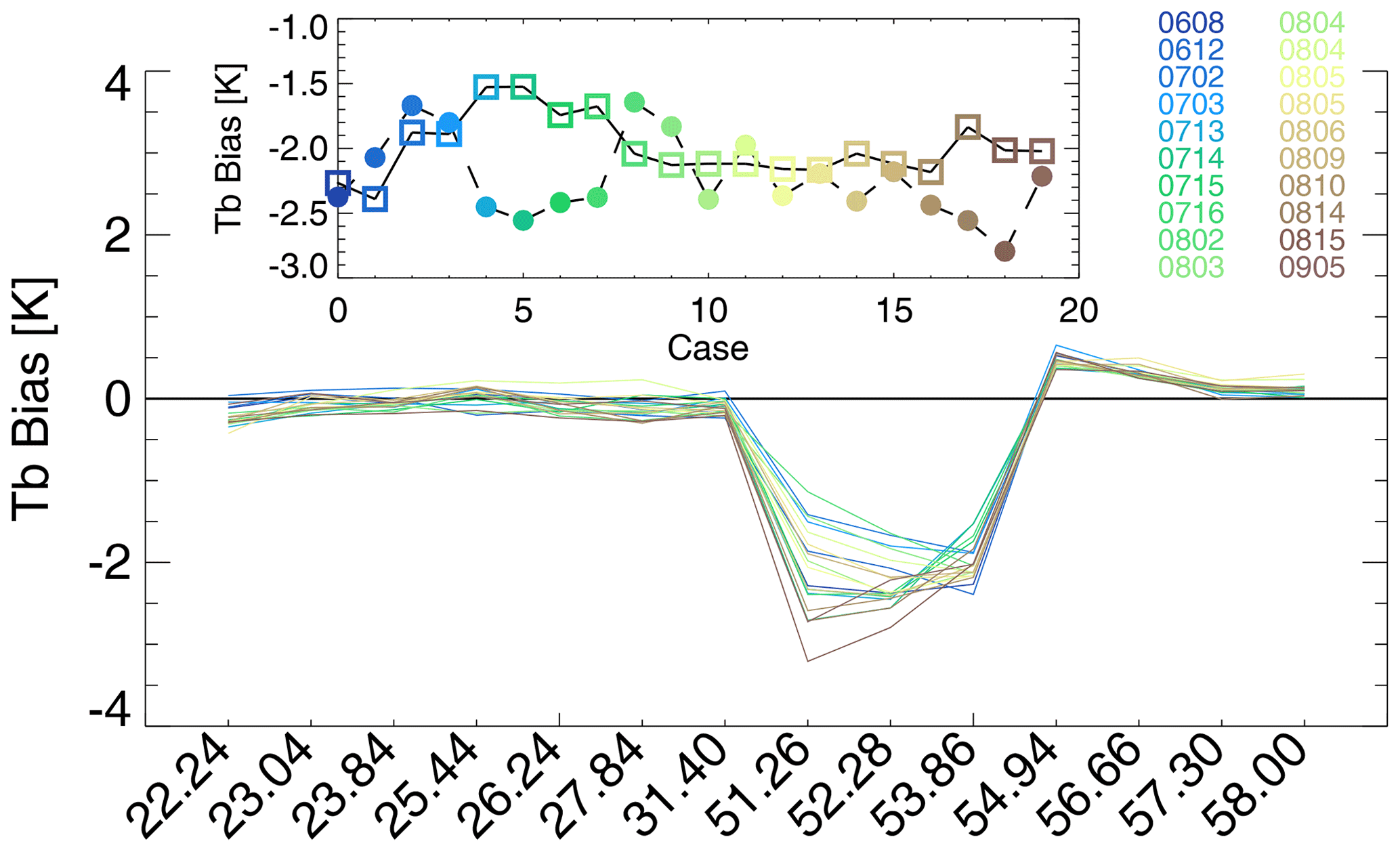
Figure A1 The T_b bias offset for the cases used in this analysis. The inset plot shows the temporal variability of the 51.26 (filled circles) and 52.28 (open squares) GHz channels for these cases, where the colours indicate the date (MMDD) of the case.

Note that we do not consider or correct for possible spectral biases in the MWR frequencies channels (Löhnert and Maier, 2012). It is possible that the large T_b biases in the 51.26, 52.28, and 53.86 GHz channels are a combination of both spectral and radiometric biases. It is important to note that the biases in those channels might not be entirely due to the calibration accuracy of the microwave radiometer; the bias could also be explained by systematic errors in the radiative transfer model used, as the various uncertainties of the absorption line properties at those frequencies results in large model uncertainty (Cimini et al., 2018).

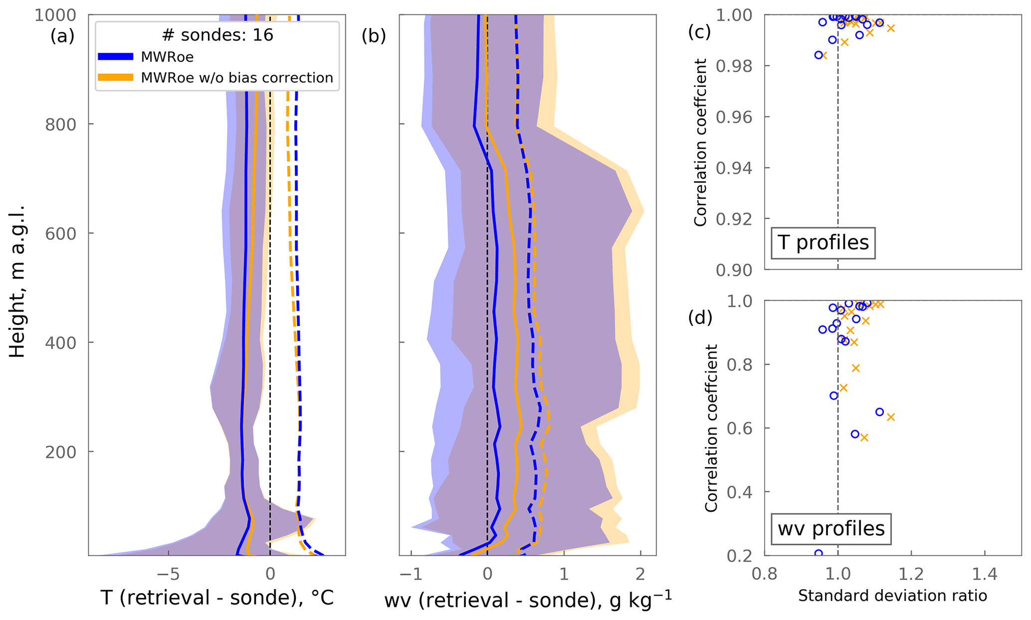
Figure A2 As Fig. 4 but comparing the performance of the final MWRoe retrieval (blue) with that of the MWRoe retrieval without the additional T_b bias correction applied (orange). The solid line shows the mean bias and the shaded represents the range. Dashed lines show the root-mean-squared error (RMSE).

Figure A2 illustrates the difference between the MWRoe-retrieved thermodynamic profile compared to the radiosondes during the radiation fog case studies with and without the mean radiosonde-derived bias correction applied. The application of the bias correction reduces the mean bias in the water vapour profile from 0.14 to 0.01 g kg⁻¹ and the mean RMSE from 0.47 to 0.43 g kg⁻¹. However, the bias correction has little effect on the temperature profiles. The reason for the consistent small negative temperature bias in the MWRoe both with (mean −1.45 ^∘C) and without (mean −1.26 ^∘C) the bias correction is currently unknown, especially since the mean T_b bias in the high-frequency end of the V-band is very close to zero.

The reduction in the bias and RMSE of the MWRoe-retrieved water vapour profile compared to the radiosondes demonstrates that the application of the additional T_b bias correction is essential for making accurate MWR thermodynamic profile retrievals. Currently, the only way of performing this bias correction is by using an alternative “truth” profile (in this case, radiosonde profiles); this is a significant disadvantage of the MWR, since radiosondes are spatially sparse, resource intensive, and expensive. However, a method using only the climatology data, as encapsulated in the a priori data, has been proposed by Djalalova et al. (2022); this new method helps to account for some of the spectral artefacts in the bias but needs additional research to help characterise any systematic error that might be introduced by the method.