the Creative Commons Attribution 4.0 License.
the Creative Commons Attribution 4.0 License.
 | 13 Sep 2022
Extending water vapor measurement capability of photon-limited differential absorption lidars through simultaneous denoising and inversion
Willem J. Marais
Matthew Hayman
The micropulse differential absorption lidar (MPD) was developed at Montana State University (MSU) and the National Center for Atmospheric Research (NCAR) to perform range-resolved water vapor (WV) measurements using low-power lasers and photon-counting detectors. The MPD has proven to produce accurate WV measurements up to 6 km altitude. However, the MPD's ability to produce accurate higher-altitude WV measurements is impeded by the current standard differential absorption lidar (DIAL) retrieval methods. These methods are built upon a fundamental methodology that algebraically solves for the WV using the MPD forward models and noisy observations, which exacerbates any random noise in the lidar observations.
The work in this paper introduces the adapted Poisson total variation (PTV) specifically for the MPD instrument. PTV was originally developed for a ground-based high spectral resolution lidar, and this paper reports on the adaptations that were required in order to apply PTV on MPD WV observations. The adapted PTV method, coined PTV-MPD, extends the maximum altitude of the MPD from 6 to 8 km and substantially increases the accuracy of the WV retrievals starting above 2 km. PTV-MPD achieves the improvement by simultaneously denoising the MPD noisy observations and inferring the WV by separating the random noise from the non-random WV.
An analysis with 130 radiosonde (RS) comparisons shows that the relative root-mean-square difference (RRMSE) of WV measurements between RS and PTV-MPD exceeds 100 % between 6 and 8 km, whereas the RRMSE between RS and the standard method exceeds 100 % near 3 km. In addition, we show that by employing PTV-MPD, the MPD is able to extend its useful range of WV estimates beyond that of the ARM Southern Great Plains Raman lidar (RRMSE exceeding 100 % between 3 and 4 km); the Raman lidar has a power-aperture product 500 times greater than that of the MPD.
- Article
(9970 KB) - Full-text XML
- BibTeX
- EndNote


Water vapor (WV) is one of the fundamental thermodynamic variables that defines the state of the atmosphere and influences many important processes related to weather and climate. The importance of continuously monitoring lower tropospheric WV is underscored in the National Aeronautics and Space Administration (NASA) decadal survey (National Academies of Sciences, Engineering, and Medicine, 2018b) and in National Research Council (NRC, 2009, 2010, 2012) and National Academy of Sciences (National Academies of Sciences, Engineering, and Medicine, 2018a) reports. In particular, continuous range-resolved measurements of WV are needed at large scales to improve severe weather and precipitation predictions (Weckwerth et al., 1999; Wulfmeyer et al., 2015; Geerts et al., 2016; Jensen et al., 2016).
To fulfill this observational need, Montana State University (MSU) and the National Center for Atmospheric Research (NCAR) have developed a micropulse differential absorption lidar (MPD) that continuously measures range-resolved WV in the lower (150 m to 6 km) atmosphere (Spuler et al., 2015, 2021; NCAR/EOL MPD Team, 2020). The MPD is designed for unattended network deployment, using low-power, low-cost, high-reliability diode lasers that enable class 1M eye-safe transmitted lasers. The MPD employs the narrowband differential absorption lidar (DIAL) technique on a WV absorption line with low temperature sensitivity, whereby approximate knowledge of atmospheric temperature and pressure allow for a first-principles-based retrieval (Nehrir et al., 2009). An immediate benefit of the MPD is that it provides continuous WV measurements independent of radiosonde WV measurements, which can provide additional information to numerical weather prediction (NWP) data assimilation systems.
1.1 Problem statement – extending capability of MPD
The MPD has proven to produce accurate WV measurements up to 6 km altitude, depending on aerosol loading, clouds, and solar background. However, in high solar background conditions, MPD water vapor retrievals can be noisy as low as 2 km. The MPD's ability to produce precise measurements above 2 km and accurate higher-altitude WV measurements is impeded by the current standard WV DIAL retrieval methods. These methods are built upon a fundamental methodology that algebraically solves the WV variable through operations that exacerbate any random noise in the lidar observations (Marais et al., 2016). To suppress the noise the standard method applies low-pass filters on the algebraically computed WV using a Gaussian smoothing kernel or Savitzky–Golay filter (Schafer, 2011). The signal-to-noise ratio (SNR) of the WV measurements can be further improved upon by reducing the vertical and horizontal resolutions of the photon-counting observations. However, reducing the resolutions introduces systematic biases in the WV due to the nonlinearity of the single-scatter lidar equation. Smoothing operations are limited in their benefits because optimal averaging is generally localized to patches of correlated structure in a lidar profile. Invariably, parts of the profile are over-smoothed (resulting in biases), while other parts are under-smoothed (resulting in random error) (Hayman et al., 2020).
Figure 1 illustrates the shortcomings of low-pass filtering, where Fig. 1b and e show the standard method estimated WV image and profile obtained using low-pass filtering. The profile is juxtaposed with a coincident radiosonde (RS) WV profile. Although the bandwidth of the low-pass filter is relatively well suited for low altitude (≤ 4 km) WV measurements, Fig. 1i shows that the filter is not sufficient to meaningfully reduce the noise at higher altitudes. Furthermore, Fig. 1ii illustrate that the low-pass filter also over-smooths rapidly changing WV features such as embedded dry regions.

Figure 1The (a) attenuated-backscatter cross section (atten. backs.) and the water vapor (WV) measurements of the (b) standard (STND) and (c) PTV-MPD methods. Panel (a) is not masked to show what atmospheric features have been masked out in (b) and (c) by the gray areas. The dashed vertical white lines in (b) and (c) show the launch time of the radiosonde (RS), where (e) and (f) show the RS WV profile. Panel (e) compares the standard method WV measurements with RS WV profile, whereas (f) shows the same comparison for the PTV-MPD method. The horizontal dashed lines in (e) to (f) show the altitude at which the RS was horizontally 5 km away from the MPD. The dashed boxes in (e) and (f) highlight regions that are discussed in the text.
1.2 Proposed approach to extending MPD capability
Advances have been made in denoising photon-counting medical images where the photon detection methodologies and forward modeling are similar to that in atmospheric lidar (Fessler, 2020; Oh et al., 2013; Harmany et al., 2012; Willett and Nowak, 2003; Ahn and Fessler, 2003). Basically, these methods quantitatively separate the image being estimated from the random noise by making a distinction between the (1) vertical and horizontal correlations among the pixels of the underlying image and (2) the uncorrelated photon-counting noise. The work of Xiao et al. (2020), Hayman and Spuler (2017), and Marais et al. (2016) have demonstrated that the medical denoising methods can be adopted and adapted to dramatically improve the inference of the extinction cross section from ground-based photon-counting high spectral resolution lidar (HSRL).
Inspired by the medical image denoising methods and the Poisson total variation (PTV) method for inferring extinction from HSRL observations (Xiao et al., 2020; Hayman and Spuler, 2017; Marais et al., 2016), we explore how the PTV method can be adapted for the MPD instrument to extend its capability for measuring WV. Figure 1c and f show an example WV measurement of the adapted PTV method, labeled as PTV-MPD, of the same scene and profile of Fig. 1c and e; using the range intervals indicated by Fig. 1i and ii, the PTV-MPD WV measurements are more accurate at higher altitudes and at the embedded dry region compared to the standard method.
The PTV-MPD method we present in this paper differs from PTV by three adaptations that are necessary for accurate WV measurements (Marais et al., 2016).
-
Forward models for DIAL. The first adaptation of PTV requires that we develop MPD forward models to fit the estimated parameters on to the observed photon counts; while the objective is to estimate the WV, to accommodate the forward model, the attenuated backscatter is also an estimated product. To accurately model what the MPD observes, a convolution operator is included in the forward model that represents the oversampling of the laser pulse (Spuler et al., 2021); the MPD uses relatively long laser pulses to increase the SNR, with the trade-off of blurring the backscatter optical signal described by the standard single-scatter lidar equation (SSLE).
-
Simultaneous inference. PTV for the HSRL infers the backscatter and extinction cross sections with a two-step approach in order to isolate geometric overlap calibration biases to the extinction cross section. However, with PTV-MPD a two-step approach is not necessary to infer the WV and attenuated backscatter since the DIAL employs a differential measurement technique, which decouples the WV measurement from the geometric overlap. Hence, the second adaptation of PTV is that PTV-MPD infers the WV and attenuated backscatter simultaneously instead of separately. The simultaneous inference approach produces WV estimates that are more faithful to the MPD observations compared to the two-step inference approach.
-
Mitigate DIAL sensitivity to initial attenuated backscatter. The simultaneous inference of the WV and attenuated backscatter requires initial estimates of both the WV and attenuated backscatter. Our experiments show that PTV-MPD is sensitive to near-range inaccuracies in the initial attenuated-backscatter estimate, which induces inaccuracies in the near-range WV measurements. Therefore, the third adaptation involves making PTV-MPD more robust against inaccuracies in the initial attenuated backscatter.
1.3 Contributions
The immediate contributions of this paper are the
-
adaptation of the PTV method (i.e., PTV-MPD) for the DIAL technique and
-
the first rigorous validation of the PTV method using in situ measurements.
This work also serves as an example of how development of advanced signal processing can provide insights into improving hardware design and trades. By leveraging advances in signal processing, lidar hardware costs might be reduced whilst maintaining or improving the retrieval precision.
1.4 Outline, notation, and symbols
We introduce the MPD forward models in Sect. 2. Thereafter, in Sect. 3 we discuss the noise model of the MPD and how saturated photon counts are masked. The standard and PTV-MPD methods are discussed in Sects. 4 and 5. The paper ends with experiment results in Sect. 6 and the conclusion thereafter.

Geophysical variables and the lidar forward models are written as matrices. When we introduce a geophysics-related variable we immediately indicate the units of the variable using the notation [⋅]; for example [W]. Table 1 lists the primary matrices and index variables used throughout this paper. The nth row and kth column element of a matrix is denoted, for example, by φn,k. We use the superscript index (ι) to indicate whether a matrix or vector is specific to lidar channel (i.e., wavelength).
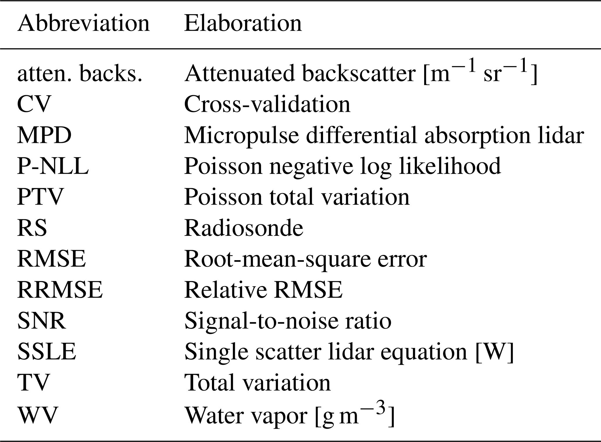
Table 2 lists commonly used acronyms that are being used throughout this paper.
To date NCAR has five experimental MPD instruments where each instrument transmits laser pulses at a rate of 7 to 8 kHz at two wavelengths sequentially. The first wavelength is tuned on a WV absorption line near 828.2 nm, whereas the second wavelength is off an WV absorption line near 828.3 nm (Spuler et al., 2015); these wavelengths are indexed by . The MPDs transmit laser pulses that are longer than the sampling interval Δt=250 ns to increase the SNR of the WV measurements; the laser pulse duration was 1 µs during a Southern Great Plains (SGP) field campaign and has recently been decreased to 625 ns for the next generation of MPDs (Spuler et al., 2021). The integer ΔN≥0 quantifies how many vertical sampling intervals Δt, minus 1, fit in the duration of a laser pulse; for example, for the SGP data .
The MPD instrument photon detector observes the weighted sum of the lidar equation and the laser pulse, since the laser pulse spans multiple range sampling intervals. We define the SSLE on the measurement range axis, which are denoted by where . The MPD samples the photon rates mid-duration of the laser pulse, and therefore the range axis of the observations is shifted relative to the measurement range axis. Specifically, the observation range axis is denoted by , where indexes the observation range axis; the relation between the observation and measurement range axes is
The SSLE is a function of the unknown WV [g m−3] and uncalibrated attenuated backscatter [m−1 sr−1], where the columns of the matrices are indexed by . We write the SSLE as a matrix function since our attention is on inferring an image of the WV. The single-scatter lidar matrix function at measurement range for channel ι is denoted by
and its unit is [W]. The calibration parameters are the range resolution m, backscatter calibration constant [J sr m3], and geometric overlap . The WV absorption [m2 g−1] of channel ι is denoted by and is pre-computed using (1) an assumed lapse rate with which the temperature and pressure profiles are approximated, (2) the mass of a water molecule per mole, and (3) the Avogadro number (Spuler et al., 2015; Nehrir et al., 2009).
The weighted sum of the SSLE with the laser pulse is modeled by
where the matrix models the laser energy distribution over the multiple range sampling intervals; the factor Δt models the integration of the observed photon rate by the photon detectors. The first ΔN+1 columns () of the first row (n=1) of the matrix is the fractional laser energy distribution over the duration of the pulse such that the sum of the first row is equal to one, and the remaining N columns are equal to zero. The nth row of matrix is the first row of shifted circularly to the right n times. Hence, the MPD forward model at range for channel ι is defined by
where Uk is the number of laser shots per column index k. The vector is the dark and solar background photon rate [W] of channel ι.
The MPD instrument photon detectors are saturated over several range bins after each laser shot due to internal scattering in the co-axial optical configuration. Consequently, the first WV estimate starts at 125 m or 500 m depending on the hardware configuration. To model the unobserved WV from range 0 up to r1, the lowest water absorption cross section is the range axis sum of the absorption cross sections from range 0 up to r1. Hence, the WV φ1,k at range r1 represents the range-average WV from range 0 up to r1.
3.1 Photon-counting noise probability mass function
The photon-counting observations at range and profile k of the online and offline channels are denoted by . Each photon count represents temporally accumulated counts of multiple laser shots as indicated by Uk. The noise of the photon counts are modeled by the Poisson probability mass function (PMF) if the corresponding photon rates are below the saturation limit of the MPD photon detectors (Donovan et al., 1993; Müller, 1973). The expected values of these unsaturated photon counts is modeled by the MPD forward model Eq. (5), and we assume that
where
3.2 Masking saturated photon counts
The instantaneous backscattered photon rates, corresponding to each laser shot, of clouds and precipitation can exceed the MPD photon detector saturation limit. Moreover, the accumulated photon counts consists of a combination of unsaturated and saturated photon counts within and at the edges of clouds and precipitation. Photon counts that are saturation contaminated cannot be accurately modeled by the Poisson PMF (Donovan et al., 1993). Hence, saturated photon counts and corresponding forward model pixels are excluded from our inference methodology using a mask matrix Mn,k.
The saturated photon count mask Mn,k has to be constructed via proxy data that indicate whether the instantaneous backscattered photon rates exceed the photon detector saturation limit. Since we know a priori that dense aerosol layers, clouds, and precipitation have large backscatter cross sections, the matrix Mn,k masks out these atmospheric features.
We used a sliding window standard deviation filter on the photon counts , with a fixed threshold, to identify the large backscatter cross sections of dense aerosol layers, clouds, and precipitation; the threshold was set by qualitatively validating whether these large backscatter cross sections have been masked out.
3.3 Photon-counting noise negative log likelihood
The Poisson negative log likelihood (P-NLL) is used by the PTV-MPD method to quantify the fitting of the WV and attenuated backscatter onto the noisy observations via the MPD forward model Eq. (5). The P-NLL function of channel ι is denoted by
where p is a normalization factor that is used in conjunction with the photon counts. The saturated photon counts are masked out with the matrix Mn,k. The factorial term of the Poisson PMF is omitted in Eq. (8) since it is a constant value.
A detailed discussion of the standard processing technique employed for MPD is provided in Spuler et al. (2021). Nonetheless, we will provide a brief overview of the method here as outlined in Alg. 1.
Algorithm 1The MPD standard method.
The photon count profiles first undergo low-pass filtering to suppress the random noise (Hayman et al., 2020). The ratio of the online and offline channels cancels the attenuated backscatter in each forward model, which allows us to solve directly for the optical depth resulting from WV. At this stage, the WV estimate has residual noise that is low-pass-filtered with Gaussian kernels, with 5 to 10 min by 170 m bandwidths, to further reduce the noise in the observation. The smoothing kernel of the low-pass filter is fixed across the scene. Thus, the WV estimates are often over-smoothed in highly dynamic, high-SNR regions and under-smoothed at higher altitudes. Due to the direct nature of the inversion, there are also no constraints imposed on the retrieval, therefore nonphysical WV estimates are frequently obtained in noisy regions. The nonphysical WV values, in turn, can create problems in further downstream scientific analysis where nonphysical state variables present a challenge. Nonphysical quantities are generally not easily included in such analysis, but the selective omission or limiting of nonphysical noise will also create biases.
Finally, the lengths of the laser pulses are not accounted for in the standard method. Specifically, inclusion of the laser pulse in the forward model prevents the attenuated-backscatter term from directly canceling out when dividing the offline with the online channel, and a direct inversion becomes no longer possible. However, failing to account for the laser pulse length can create biases in some cases, for example at WV dry regions.
The PTV method, originally developed for photon-counting HSRL (Marais et al., 2016), is an adaptation of the SPIRAL method, which is a regularized maximum likelihood technique (Oh et al., 2013; Harmany et al., 2012); the technique and derivations of it have be applied in wide range of inverse problems in different domains, such as in medical imaging and astronomy (Roelofs et al., 2020; Harmany et al., 2012).
5.1 Overview of PTV
With PTV the assumptions are that
-
the photon-counting noise can be accurately modeled by the Poisson PMF in Eq. (6),
-
the expected value of the photon counts can be accurately modeled with a forward model (i.e., Eq. 5), and
-
the geophysical variable (i.e., WV) image that we want to estimate can be accurately approximated with a two-dimensional (2D) piecewise constant (PC) function.
An accurate noise model is important in inverse problems, since with Poisson noise the noise variance is signal dependent, and modeling the photon-counting noise as a Gaussian distribution will lead to inversion inaccuracies (Harmany et al., 2012). The 2D PC approximation induces spatial correlations on the estimated geophysical variable while preserving any discontinuities; such correlations are expected from the true unobserved geophysical variable of which WV and attenuated backscatter are examples.
By making a distinction between the random noise and the geophysical variable having spatial correlation, PTV is capable of separating the noise from the geophysical variable that is being estimated. PTV achieves this separation by (1) using the P-NLL from Eq. (8) to quantify how close of a fit the forward model is relative to the noisy observations and by (2) employing the total variation (TV) penalty function that regularizes the geophysical variable to be approximately 2D PC.
The approach used by PTV is formulated as a mathematical optimization framework where we search over all candidate geophysical variables and choose the geophysical variable that minimizes the sum of the (1) P-NLL composited with the forward model and (2) the TV penalty functions. The P-NLL composite is called the “loss function” and the loss summed with the penalty functions is called the “objective function”. The optimization framework is conceptually illustrated by the equation
where X ≡ geophysical variable, Y ≡ photon-counting observations, ≡ P-NLL composited with forward model, e.g., Eq. (8).
The (anisotropic) TV penalty function is defined as (Harmany et al., 2012)
and is weighted with a tuning parameter that sets the degree to which the 2D PC regularization is promoted. The tuning parameter is quantitatively determined through a cross-validation methodology (Friedman et al., 2001, chap. 7)(Oh et al., 2013), and the parameter is not set by “expert opinion”.
5.2 PTV-MPD: adaptation required for MPD
We adopt the PTV method to infer the WV from the MPD observations, where we approximate both the WV and attenuated backscatter as 2D PC functions. In contrast, the standard method of Alg. 1 divides out the attenuated backscatter, which is not feasible with PTV-MPD since it is unclear how to model the noise of the ratio of background subtracted photon counts.
In order to apply PTV on MPD observations the following adaptations are required:
- (A1)
-
use of the MPD forward models of Eq. (5),
- (A2)
-
allowing for the simultaneous inference of the WV and attenuated backscatter.
- (A3)
-
prevention of the degradation of the WV measurement due to inaccuracies in the initial attenuated-backscatter value.
Adaptations (A1) and (A2) are achieved by redefining the PTV loss and objective functions, as discussed in the next section. Specific to adaptation (A2) in the original HSRL formulation of PTV, (1) the backscatter cross section was computed from the denoised photon counts, and (2) the lidar ratio was inferred using the computed backscatter cross section. This two-step sequence isolates calibration biases due to the geometric overlap function from the inferred lidar ratio and the extinction cross section. With a DIAL instrument such as MPD, the geometric overlap does not induce a bias in the inferred WV, in part because both measurements use the same photon detector (Spuler et al., 2015, 2021). Therefore, the two-step sequence used for HSRL observations is not necessary.
Regarding adaptation (A3), the simultaneous inference of the WV and attenuated backscatter requires an initial value of the attenuated backscatter. During our investigation of adapting PTV for the MPD instrument we noticed that the adapted PTV method is sensitive to inaccuracies in the initial attenuated-backscatter value. Specifically, when computing the initial value of the attenuated backscatter algebraically from the photon-counting observations, the contributions to the inaccuracies in the initial attenuated backscatter originate from the small SNR at close ranges and the long laser pulses that convolve with the SSLE (see Eq. 4). Hence, for adaptation (A3) we propose that PTV-MPD employ a coarse-to-fine image resolution framework when inferring the WV (Marais and Willett, 2017). With the coarse-to-fine framework, we first infer the WV and attenuated backscatter at a coarse image resolution, which allows for reducing inaccuracies in the initial attenuated backscatter. In other words, at the coarse image resolution the long laser pulses are deconvolved from the initial attenuated backscatter and the SNR of close-range observations are implicitly increased. In a sequence from coarse-to-fine image resolution, we use the coarse-resolution WV and attenuated-backscatter estimates as initial values when inferring the finer image resolution WV and attenuated backscatter.
5.3 PTV-MPD method algorithmic details
Using the conceptual optimization framework in Eq. (10) as a reference, the PTV-MPD method is formulated as an optimization problem where the minimizers of the objective function are the estimates of the WV φ and attenuated backscatter χ. The objective function used by PTV-MPD is introduced in Sect. 5.3.1, which addresses adaptations (A1) and (A2); Sect. 5.3.1 serves as a preliminary section before elaborating on the coarse-to-fine image resolution framework. Minimizing an objective function requires initial values of the WV φ and attenuated backscatter χ and can have a significant impact on the estimate of these variables (Harmany et al., 2012; Kelley, 1999); to this effect, in Sect. 5.3.2 we discuss the initial values of the WV φ and attenuated backscatter χ. Finally, Sect. 5.3.3 discusses how the objective function is minimized through the coarse-to-fine image resolution framework that addresses adaption (A3).
The formulation of the PTV-MPD includes tuning parameters that are computed using a cross-validation (CV) methodology; the CV involves calculating a validation error that indicates the optimality of the tuning parameters and is discussed in Sect. 5.3.4. Related to the tuning parameters and validation error, we require a way to test the hypothesis that the coarse-to-fine image resolution framework will improve the accuracy of inferring the WV φ. To test the hypothesis, we compare the test errors from inferring the WV φ at only the finest image resolution versus from a coarse-to-fine image resolution. The test error computation is also discussed in Sect. 5.3.4.

Figure 2Pictorial overview of Alg. 2 and its sub-algorithms (Algs. 3 and 4) for inferring the water vapor (WV) and uncalibrated attenuated-backscatter cross section (atten. backs.). The corresponding algorithm line numbers for each block in the flow diagrams are indicated by the vertical text Lx-y. The blue, violet, and red text is meant to highlight statistically independent datasets generated using Poisson thinning.
Figure 2 gives a broad pictorial overview of how each part of the PTV-MPD framework is implemented with modularized sub-algorithms; the purposes of the sub-algorithms are as follows.
- Fig. 2a, Alg. 2
-
performs the necessary preparations to infer the WV φ and attenuated backscatter χ which includes computing the initial attenuated backscatter.
These algorithms are outlined in Sect. 5.3.5, which includes specific details about the SPIRAL method adaptations.
5.3.1 Preliminary for coarse-to-fine framework: the loss and objective functions
The PTV-MPD loss function differs from the PTV loss function in two respects; cf. Eq. (23) in Marais et al. (2016). First, the loss function of PTV-MPD is defined such that we infer the log e of the attenuated backscatter denoted by , since previous work suggests that more accurate inference can be achieved by inferring the log e of a linear variable with methods similar to PTV (Oh et al., 2013, 2014). Second, we define the PTV-MPD loss function as the sum of the normalized P-NLL function of each channel, where the normalization ensures that each P-NLL function is equally weighted; this weighting is done since the accumulated photon counts of the offline channels are generally larger than that of the online channel. Hence, the PTV-MPD loss function is defined by
which is the weighted sum of the P-NLL of each channel where each P-NLL is normalized by the root sum square (i.e., Frobenius norm) of the photon counts that have not been masked out. The Frobenius norm of the mask photon counts is defined by
The objective function that is minimized by PTV-MPD is defined as
which is parameterized with the WV φ and attenuated backscatter and their respective tuning parameters λw and λa. The WV λw and attenuated backscatter λa tuning parameters set the degree to which these parameters should be regularized to be 2D PC. While minimizing the objective function (14), the WV φ is constrained to be non-negative, which is denoted by the set 𝒲. The objective function (14) is minimized using the alternating minimization method in conjunction with adaptations of SPIRAL (Beck and Tetruashvili, 2013; Harmany et al., 2012); the alternating minimization is elaborated in Sect. 5.3.5 and outlined by Alg. 4.
5.3.2 Initial values of objective function
In Appendix B we show that for low-SNR regions of the photon-counting images there can be multiple estimates of the WV φ or attenuated backscatter that minimizes the objective function (14). The dark and solar background photon rates b(ι) are the primary factors that determine the domains over which the objective function has a unique minimizer. Consequently, we expect that PTV-MPD will require accurate initial values of the WV φ and attenuated backscatter whenever the photon count SNRs are dominated by the background rate b(ι) such as at close range and in high-altitude regions.
It will be advantageous for the MPD to make WV measurements that are statistically independent of RS for the purpose of providing additional statistically independent information for NWP data assimilation. Thus, in this paper we set the initial WV to zero [g m−3]; this WV initial value reflects that we assume no a priori information about the WV other than (1) the assumed lapse rate1 of the atmosphere and (2) the assumption that the WV can be accurately approximated with 2D PC functions. This initial WV value is denoted by .
The offline channel is less sensitive to WV absorption compared to the online channel. Hence, the initial value of the attenuated backscatter, denoted by , is computed from the offline channel with the initial WV via
The matrix AT maps the observations to the measurement space; the matrix is the adjoint (i.e., transpose) of the laser energy distribution matrix A. The vector U is the number of accumulated laser shots, and Δt models the integration of the observed photon rate by the photon detectors (see Sect. 2).
5.3.3 The coarse-to-fine inference framework
With the coarse-to-fine image resolution inference framework, we start with estimating a coarse-resolution WV image and use the coarse-resolution estimate as an initial WV value at a finer image resolution; this technique has proven useful to more accurately denoising and inverting images for low-SNR photon-limited application (Marais and Willett, 2017; Azzari and Foi, 2017). The coarse image resolution estimation is akin to downsampling the noisy observations to increase the SNR, though the difference is that with the proposed methodology the downsampling in the coarse-to-fine framework takes into account the MPD forward model (5).
Following the approaches delineated in Marais and Willett (2017) and Azzari and Foi (2017), we define the following variables and linear operators.
-
A series of values that represents the downsampling factors of the coarse-to-fine image resolutions at which the WV will be inferred; represents the coarsest image resolution.
-
The downsampling operator is denoted by and its corresponding upsampling operator .
The downsampled image will have approximately rows and columns, depending on how the downsample operator handles boundary pixels. The coarse-resolution WV image is denoted by ϕh, and its relationship with the finest image resolution WV image φ is governed by the upsampling operator where . The corresponding attenuated backscatter is denoted by ψh and is not downsampled like the WV; the subscript h in ψh indicates that it is paired with the downsampled WV ϕh estimate.
Let represent the coarse-to-fine image resolution index. The coarse-to-fine process repeats the following steps for each l until the finest image resolution WV estimate is obtained.
Step 1. Define the current image resolution WV estimate and its paired attenuated-backscatter estimate . In addition, define the current image resolution objective function.
Step 2. If l=1, use the provided initial value of the WV and attenuated backscatter when minimizing the objective function (16). Otherwise, use the previous image resolution estimates as initial values for the current image resolution. Specifically, the initial value for the WV is , and for the attenuated backscatter it is .
Step 3. Estimate the current image resolution WV and its paired attenuated backscatter by minimizing the objective function (16):
where 𝒲 is the set of non-negative numbers.
Final step. If l=L, the final WV and attenuated-backscatter estimates are denoted by and meaning
and
The subscripts , λw and λa indicate that the estimates of the WV φ and attenuated backscatter are the specific to coarse-to-fine image resolution configuration parameterized by and the tuning parameters λw and λa.
In practice, the minimization of the objective function (16) is done by alternating minimization between the WV and attenuated backscatter as indicated in Fig. 2c and outlined by Alg. 4.
5.3.4 Computing validation error to choose optimum tuning parameters and computing test error
The validation and test errors are computed by basically comparing the WV φ and attenuated backscatter estimates against noisy observations that are statistically independent of these estimates. This is achieved by thinning the non-masked offline Y(off) and online Y(on) photon counts through the Poisson thinning technique (Marais et al., 2016; Oh et al., 2013; Hayman et al., 2020); these thinned photon counts are statistically independent of each other and are Poisson distributed (Cinlar, 2013, chap. 4). Specifically, for each non-masked pixel in a photon-counting image Y(ι), the Poisson thinning technique randomly samples the individual photon counts, and the sampled photon counts are placed in three photon-counting images. We call these three images the training , validation , and test photon-counting images. The expected value of the training, validation, and test photon counts relative to the original photon counts are expressed by the scalars , such that , where and are similarly defined.
Training photon counts
The training photon counts are used to infer the WV and attenuated backscatter for specific WV λw and attenuated backscatter λa tuning parameters and coarse-to-fine configuration . Specifically, when using the training photon counts the objective function in Eq. (16) will be equal to
where p in Eq. (16) has been replaced with ptrn.
Validation photon counts
The validation error of the estimates per tuning parameter is computed with the P-NLL (8) and the forward model (5) and is denoted by
The optimum tuning parameters corresponds to the smallest validation error, and this give us the WV and attenuated backscatter estimates
Test photon counts
The test error for the estimates and are also computed with the P-NLL (8) and the forward model (5) and is denoted by
To test the hypotheses as to whether the coarse-to-fine image resolution framework does improve the WV measurements, we evaluate the inequality
5.3.5 The PTV-MPD algorithm
Algorithm 2 and its sub-algorithms (Algs. 3 and 4) outline the PTV-MPD algorithms as described by Fig. 2. Algorithm 2 takes as input the photon counts and the coarse image resolution at which PTV-MPD will start inferring the WV; the starting image resolution is expressed as a downsampling factor . Algorithm 3 outlines the CV methodology, and Alg. 4 outlines the coarse-to-fine WV inference image resolution framework.
The alternating minimization of the objective function (17) (Beck and Tetruashvili, 2013), employed by Alg. 4, is achieved by adaptations of SPIRAL where each adaptation is specific to the WV and attenuated backscatter variable (Oh et al., 2013; Harmany et al., 2012). The adaptation of SPIRAL includes replacing the original objective function and gradient matrix of the loss function; Appendix A presents the loss function gradient matrix along with the Jacobian matrix of the MPD forward model. The stopping criteria that is employed to stop the alternating minimization iterations in Alg. 4 uses the relative distance between consecutive estimates at the specific coarse image resolution. In more detail, if between iterations t+1 and t the relative distance, i.e.,
is less than 10−5 then the loop in Alg. 4 terminates, where
Algorithm 2The PTV-MPD method.
Algorithm 3Cross-validation methodology in choosing optimum tuning parameters when inferring WV φ and attenuated backscatter χ.
Algorithm 4Coarse-to-fine image resolution framework for inferring WV φ and attenuated backscatter χ.
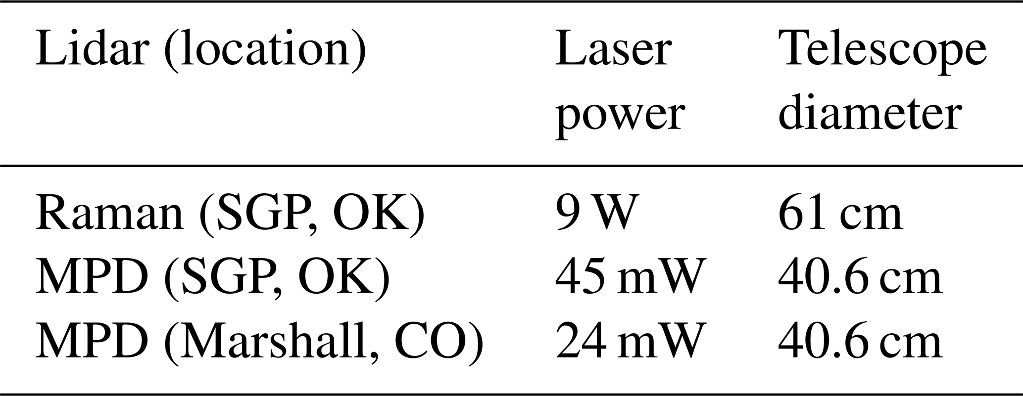
In this section we quantify the accuracy of the PTV-MPD WV measurements juxtaposed with the standard method; we use the mnemonics STND and PTV to make a distinction between the standard and PTV methods. We use RS WV measurements as an independent reference to estimate WV accuracies. The MPD with coincident RS observations was stationed (1) in proximity of the Atmospheric Radiation Measurement (ARM) SGP atmospheric observatory during spring and summer of 20192 and (2) at the NCAR Marshall field site in Boulder, Colorado, during winter and spring of 2020 and 2021 (Spuler et al., 2021). During the SGP MPD deployment, the ARM Raman lidar was making continuous WV measurements; Table 3 compares the laser power and telescope diameters of the Raman lidar and MPD.
Table 3The first column indicates the lidar instrument and where the instrument was located. SGP refers to the Southern Great Plains in Oklahoma, and Marshall refers to Marshall field in Boulder, Colorado. The second and third column show the corresponding laser power and telescope diameter.
6.1 Radiosonde comparison methodology
Although the MPD instrument was in close proximity of the ARM site during the SGP deployment, the MPD, Raman lidar, and RS instruments all observe different atmospheric volumes at different altitudes, especially in highly convective conditions. Furthermore, the Raman lidar uses some RS observations for calibration, and therefore the instrument is not entirely independent of the RS (Newsom and Sivaraman, 2018). Therefore, we indicate the altitude at which the RS is horizontally more than 5 km away from the MPD, and we also show the ARM Raman lidar WV retrievals during the SGP deployment. In contrast to the Raman lidar, the MPD retrievals or calibrations do not employ RS observations. Instead, the MPD retrievals depend on approximate temperature and pressure profiles that are computed via an assumed lapse rate, and this rate is computed from a surface observation (Spuler et al., 2015; Nehrir et al., 2009).
6.2 Data selection methodology
For the experiments we created datasets that span over specific months given (1) the high variability of WV across different months and (2) that the MPD WV measurement capability is dependent on the low-altitude WV two-way transmittance. For all the datasets presented here, the observed photon counts are binned at range and time bins of 37.5 m and 5 min, respectively. The analyzed data from SGP are not comprehensive, and we instead selected a variety of challenging cases in an effort to identify potential issues in the PTV-MPD algorithm. Specifically, much of the data targeted instances where clouds and precipitation created challenging scenes to processes.
Specific to the MPD at SGP, the WV measurements start at 500 m range due to the poor geometric overlap below this range. The next-generation MPD deployed at the Marshall field site employed optically combined telescopes with narrow and wide fields of view to improve low-altitude geometric overlap, and as a result the WV measurements start at 150 m range (Spuler et al., 2021).
Table 4The first column shows the names of the datasets used in the experiments. The second column lists the specific dates that are included in each dataset. The third and fourth columns list the number of days in each dataset and the total number of coincident RS profiles.
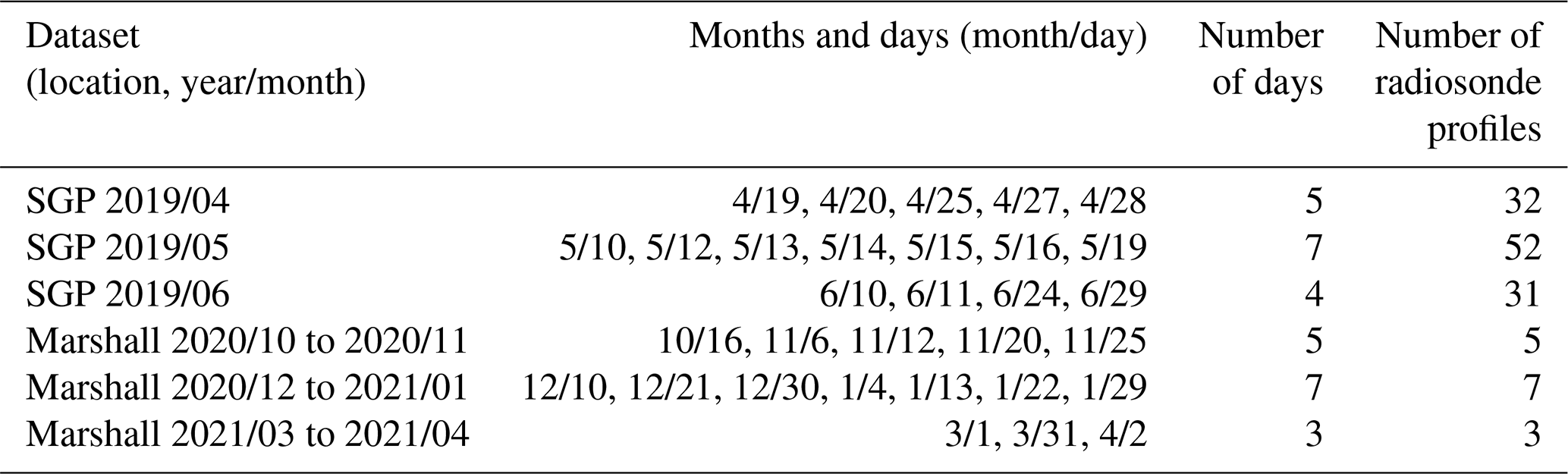
The first column of Table 4 lists the datasets, where the name of each dataset encodes the location with the year and month interval that each dataset covers. The second column lists the specific dates that are included in each dataset. The third and fourth columns list the number of days in each dataset and the total number of coincident RS profiles.
6.3 PTV-MPD tuning parameters and the coarse-to-fine (PTV-CF) configuration
The PTV-MPD method has the following input parameters, as indicated in Alg. 2:
-
the initial WV value ;
-
the WV λw and attenuated backscatter λa tuning parameters that set the degree to which the 2D piecewise constant regularization is promoted for the WV and attenuated backscatter geophysical variables (see Eq. 12);
-
the coarsest-resolution downsampling factor , which controls at what image resolution the WV inference starts at.
In addition, the PTV-MPD method depends on an input cloud mask, which in itself is set by photon rate threshold (see Sect. 3.2). As discussed in Sect. 5.3.2, the initial WV value is set to zero [g m−3]. The WV λw and attenuated backscatter λa tuning parameters are determined through a cross-validation methodology (Friedman et al., 2001, chap. 7)(Oh et al., 2013); see Sect. 5.3.4 for more detail. For all of the experiments PTV-MPD uses the default set of TV regularizer tuning parameters, which are set between lines 1 to 5 in Alg. 2.
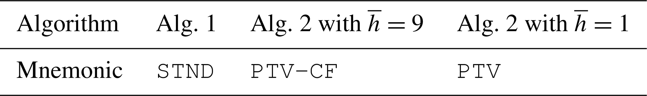
In regards to the resolution downsampling factor , we juxtapose the PTV-MPD method with () and without () the coarse-to-fine configuration to test the hypothesis of whether the PTV-MPD coarse-to-fine image resolution framework does improve the WV due to inaccuracies in the initial attenuated backscatter value. The test error (22) is used to quantify the hypotheses testing, as indicated in Eq. (23). We use mnemonics, as indicated in Table 5, to make a distinction between the two PTV-MPD configurations and the standard method. The coarse-to-fine PTV-MPD method, PTV-CF, starts at a coarse image resolution, which is 9 times () coarser than the finest image resolution.
Table 5The mnemonics used to indicate the algorithm that was used to produce a water vapor estimate. The corresponding test errors are also shown.
In the following subsection we show individual PTV-MPD WV measurement results, and thereafter we present the WV measurement error statistics.
6.4 Individual retrieval results
Figures 3
and 4 show the WV measurements obtained using the standard and PTV-MPD methods (see Table 5) when the MPD was at SGP on 11 and 10 June 2019. Figure 5 show the WV measurements when the MPD was at Marshall on 10 December 2020. These examples have been selected to highlight instances of improvement and ongoing challenges for the PTV-CF and PTV methods. For all of these figures, panel (a) shows the attenuated backscatter χ. Panels (b) to (d) show the WV φ measurements of the STND, PTV-CF, and PTV methods. The rest of the panels, i.e., (e) and beyond, show the WV profiles of the different methods compared with that of the RS and Raman lidar; the vertical dashed white lines in panels (b) to (d) show the launch times of the RSs. Panel (a) is not masked to show what atmospheric features have been masked out in panels (b) to (d) by the gray areas.
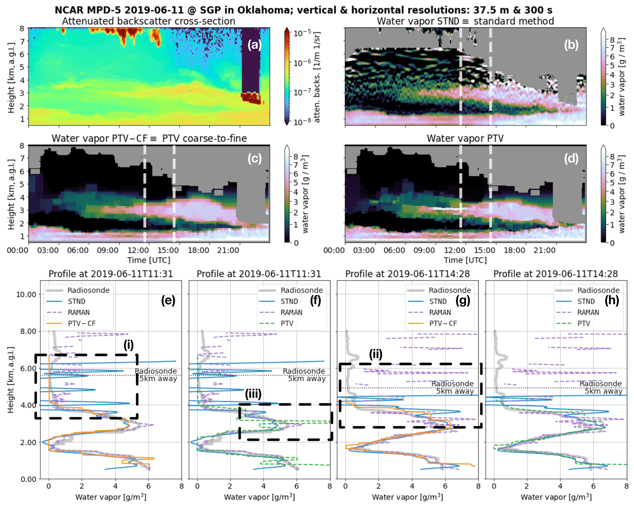
Figure 3The (a) attenuated-backscatter cross section and the water vapor (WV) measurements of the (b) standard method (STND) and the PTV-MPD method (c) with (PTV-CF) and (d) without (PTV) the coarse-to-fine configuration. Panel (a) is not masked to show what atmospheric features have been masked out in (b) to (d) by the gray areas. The dashed white vertical lines in (b) to (d) show the launch times of the radiosondes (RSs), where (e) to (h) show the RS and Raman lidar WV profiles. Panels (e) and (g) compare the course-to-fine PTV-MPD WV measurements against those of the RS and the standard method, whereas (f) and (h) show the same comparison for the PTV-MPD method without the course-to-fine configuration. The horizontal dashed lines in (e) to (h) show the altitude at which the RS was horizontally 5 km away from the MPD. The dashed boxes in (e) and (g) highlight regions that are discussed in the text.
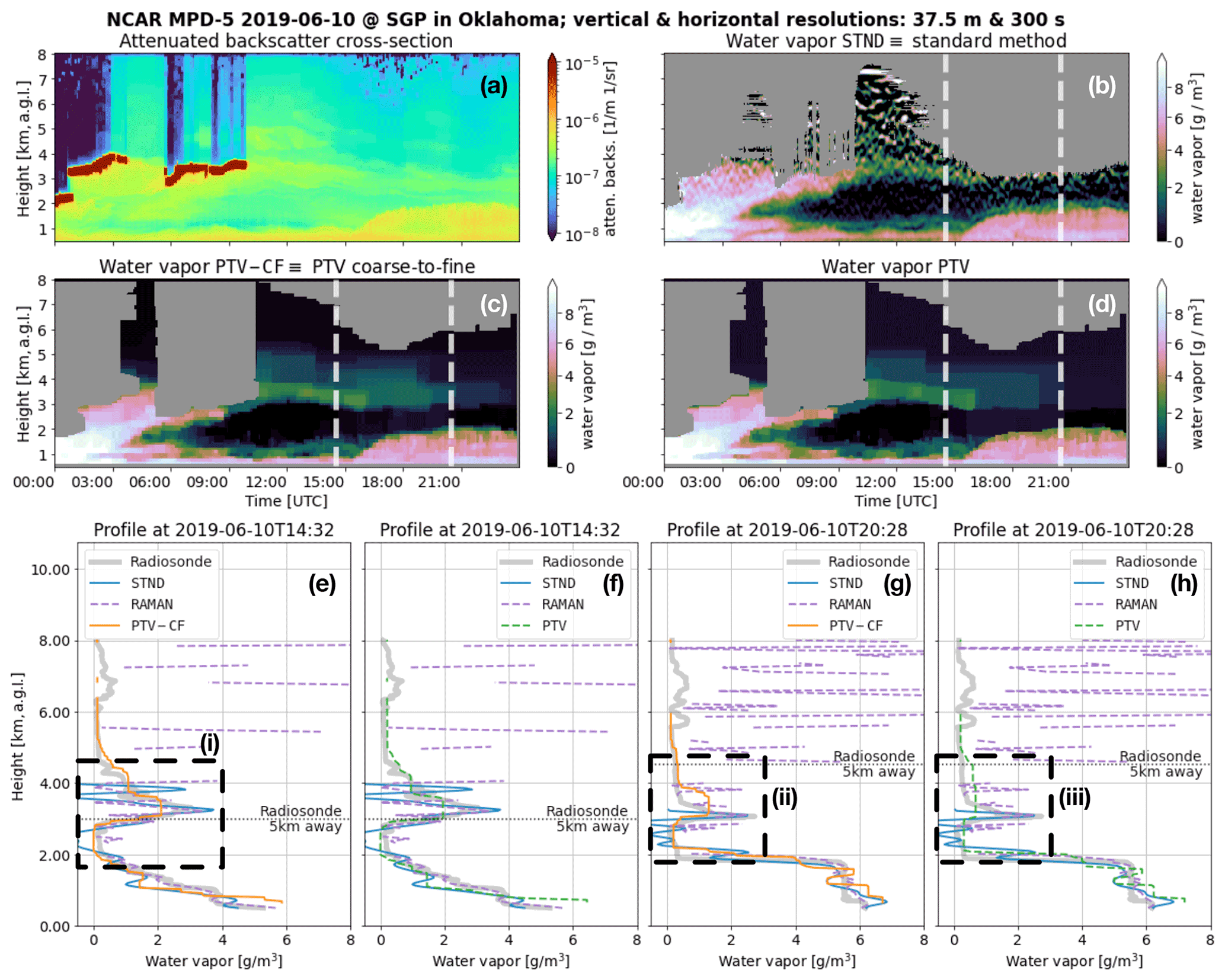
Figure 4The (a) attenuated backscatter cross section and the water vapor (WV) measurements of the (b) standard method (STND) and the PTV-MPD method (c) with (PTV-CF) and (d) without (PTV) the coarse-to-fine configuration. Panel (a) is not masked to show what atmospheric features have been masked out in (b) to (d) by the gray areas. The dashed vertical white lines in (b) to (d) show the launch times of the radiosondes (RSs), where (e) to (h) show the RS and Raman lidar WV profiles. Panels (e) and (g) compare the course-to-fine PTV-MPD WV measurements against those of the RS and the standard method, whereas (f) and (h) show the same comparison for the PTV-MPD method without the course-to-fine configuration. The horizontal dashed lines in (e) to (h) show the altitude at which the RS was horizontally 5 km away from the MPD. The dashed boxes in (e) and (g) highlight regions that are discussed in the text.
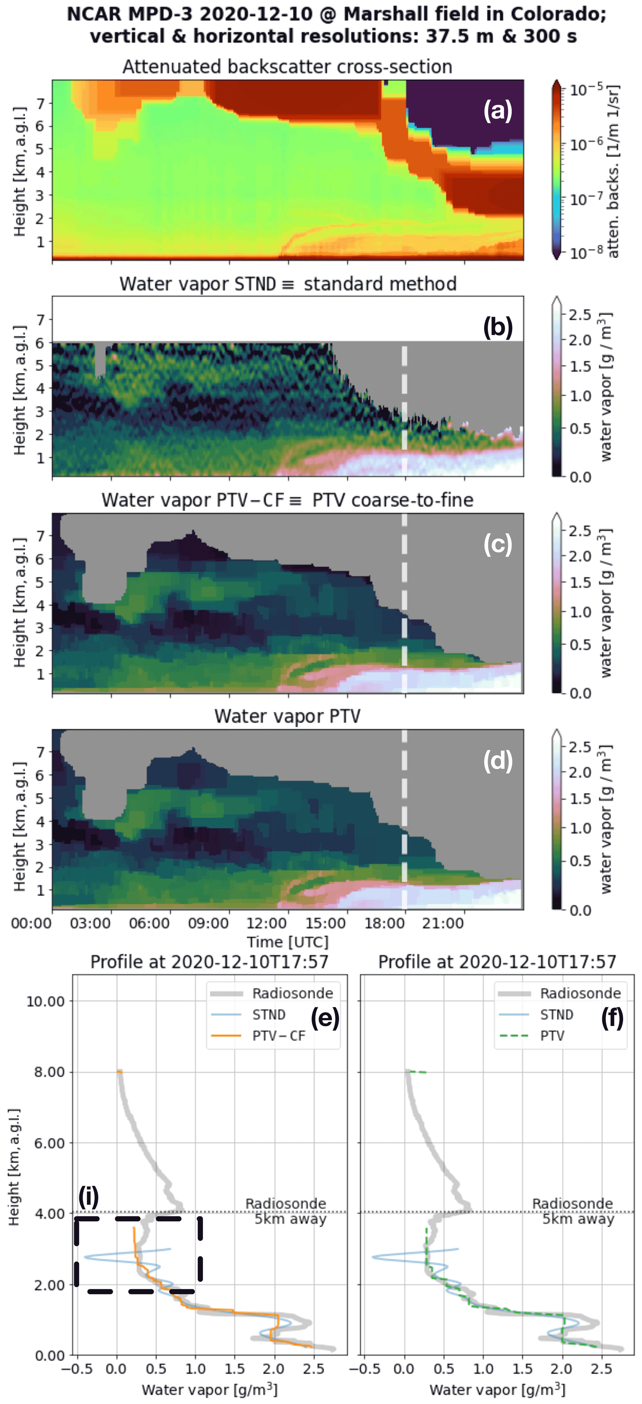
Figure 5The (a) attenuated backscatter cross section and the water vapor (WV) measurements of the (b) standard method (STND) and the PTV-MPD method (c) with (PTV-CF) and (d) without (PTV) the coarse-to-fine configuration. Panel (a) is not masked to show what atmospheric features have been masked out in (b) to (d) by the gray areas. The dashed vertical white lines in (b) to (d) show the launch times of the radiosondes (RSs), where (e) and (f) show the RS WV profiles. Panel (e) compares the course-to-fine PTV-MPD WV measurements against those of the RS and the standard method, whereas (f) show the same comparison for the PTV-MPD method without the course-to-fine configuration. The horizontal dashed lines in (e) to (f) show the altitude at which the RS was horizontally 5 km away from the MPD. The dashed box in (e) highlights a region that is discussed in the text.
6.4.1 Comparing PTV and PTV-CF with STND
When comparing the PTV and PTV-CF WV measurements with that of the STND method, the STND method exhibits higher residual noise, particularly at higher altitudes, as indicated by Figs. 3i, ii, 4i, and 5i. These oscillatory residual noise artifacts in the STND WV measurements are due to the low-pass filter that is designed for high-fidelity WV measurements up to 4 km. In contrast, the PTV-CF and PTV methods produce more accurate WV measurements at higher altitudes, and these measurements do not exhibit large residual noise artifacts. The reasons why PTV-CF and PTV make more accurate high-altitude WV measurements are as follows:
-
PTV-CFandPTVemploy the Poisson noise model with the MPD forward models to fit WV estimates onto the noisy observations, and -
the
PTV-CFandPTVmethods, via the TV regularization, exploit the spatial and temporal correlations of the WV to separate the WV from the random noise.
In some cases, residual noise in the STND method may falsely appear to capture RS observed WV structure. An example of this is shown in Fig. 4ii, where an elevated WV layer appears to be better captured by the STND method than PTV-CF, where PTV-CF identified an elevated layer that consists of lower density and greater vertical extent than the RS and Raman lidar. The uncertainty analysis available with the standard method (i.e., STND), however, shows that the noise standard deviation in the WV estimate is greater than 2 g m−3, indicating that the apparent structure is not statistically significant and is predominantly noise. This fact also becomes more apparent when viewing the time-resolved plot in Fig. 4b.
Figure 4ii demonstrates the challenge in validating the MPD profiles, particularly for regions exhibiting significant structure at higher altitudes. In this instance, the Raman lidar starts to struggle measuring WV at 3.5 km altitude during the daytime, due to the high solar background radiation noise. In order to validate such cases, the MPD, Raman lidar, and RS instruments should ideally make WV measurements of the same atmospheric volume, which is not always possible. For the purposes of the statistical analysis presented in the next section, we will nevertheless treat the RS observations as “truth” despite possible discrepancies resulting from difference in atmospheric volume.
6.4.2 Comparing PTV-CF with PTV
Comparing Fig. 3c and d we see that the PTV WV measurement appears to be larger than that of PTV-CF between 09:00 and 12:00 UTC at 3 km. Figure 3iii quantitatively shows the large PTV WV measurement, which appears to be an artifact. In contrast, the corresponding PTV-CF WV measurement in Fig. 3e is closer to RS WV. The likely cause of the artifact produced by PTV is inaccuracies in the initial attenuated backscatter that are induced by
-
the assumed WV value when computing the initial value of the attenuated backscatter (see Sect. 5.3.2) and
-
long laser pulse, denoted by operator A in Eq. (5), that is not deconvolved from initial attenuated backscatter.
Figure 4ii and iii show another distinct WV measurement difference between the PTV-CF and PTV methods. The tenuous WV identified by PTV-CF correlates more with the RS WV measurement in magnitude and shape compared to the PTV method.
The higher accuracy of the PTV-CF WV measurements corresponding to Figs. 3iii and 4iii is because the initial values of the attenuated backscatter and WV are systematically improved with the coarse-to-fine image resolution framework. Specifically, while inferring the attenuated backscatter and WV from both the online and offline channels simultaneously at the coarsest image resolution, the PTV-CF method
-
implicitly deconvolves the long laser pulse from the initial attenuated backscatter
-
and constrains the inference of the WV to be at a coarse image resolution, which implicitly increases the SNR of the observations.
6.5 Water vapor measurement error statistics
The RS WV measurements are used as a reference to produce WV measurement error statistics of the different methods discussed in the following subsection. Next, we discuss the test errors between the PTV-CF and PTV methods. We then summarize the results of the error statistics.
6.5.1 Radiosonde comparisons
For each dataset we compute the root-mean-squared “error” (RMSE) per range and the relative RMSE per range; all the methods use the same mask to exclude the same WV pixels when computing the RMSE. The RMSE and relative RMSE were computed as follows. Let denote the WV profiles inferred by one of the methods, and let denote coincident RS WV profiles. The common mask profiles are denoted by ; for example, indicates that the WV measurement at row index n is masked out by either the standard or PTV-MPD method. The RMSE and relative RMSE (RRMSE) per dataset are computed by
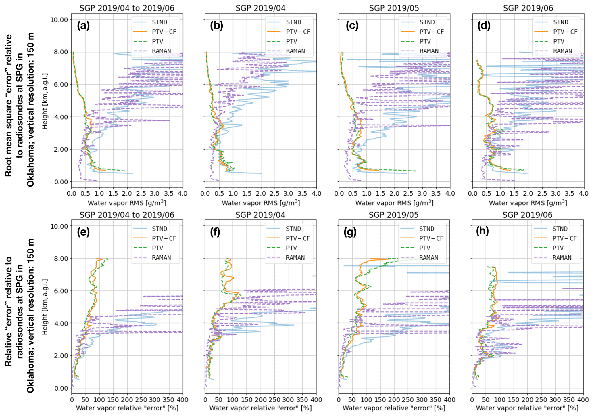
Figure 6For the all the SGP datasets, (a) shows the root-mean-square “error” (RMSE) relative to the radiosonde (RS) water vapor (WV) measurements for the standard method (STND) and the PTV-MPD method with (PTV-CF) and without (PTV) the coarse-to-fine configuration, and (e) shows the corresponding relative RMSE. Panels (b) to (d) show the RMSE for each individual SGP dataset, and (f) to (h) show the corresponding relative RMSE.
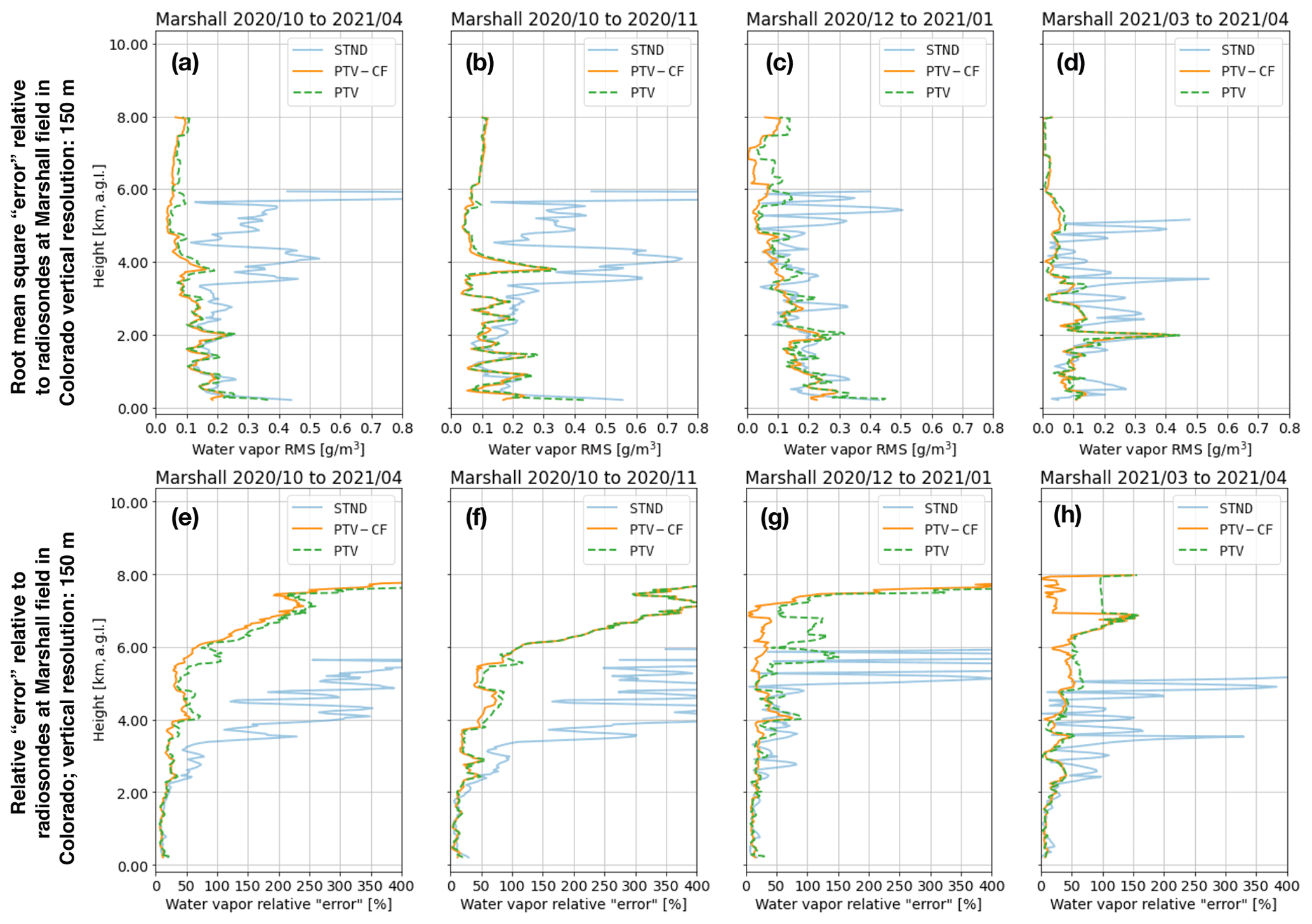
Figure 7For the all the Marshall datasets, (a) shows the root-mean-square “error” (RMSE) relative to the radiosonde (RS) water vapor (WV) measurements for the standard method (STND) and the PTV-MPD method with (PTV-CF) and without (PTV) the coarse-to-fine configuration, and (e) shows the corresponding relative RMSE. Panels (b) to (d) show the RMSE for each individual Marshall dataset, and (f) to (h) show the corresponding relative RMSE. Note that the scale of the horizontal axes in (a) to (d) are smaller than those shown in Fig. 6.
Figures 6a and 7a show the RMSE over the whole SGP and Marshall datasets, respectively, whereas Figs. 6e and 7e show the corresponding RRMSE. Figures 6b–d and 7b–d show the RMSE for each SGP and Marshall dataset (see Table 4), whereas Figs. 6f–h and 7f–h show the corresponding RRMSE.
From Figs. 6 and 7, we see that above 1.5 km the PTV-CF and PTV RMSEs and RRMSEs are comparable. Except for the lowest altitudes in Fig. 6c and d, the PTV-CF RMSEs are approximately less than 1 g m−3 for all altitudes, whereas the STND RMSE degrades with increasing altitude. For the SGP datasets, the PTV-CF and PTV RRMSEs are less than 100 % in most of the profiles up to 8 km altitude, where for the SGP 2019/04 dataset in Fig. 6f the RRMSE peaks at 125 % near 6 km altitude. The PTV-CF and PTV RRMSEs for the Marshall datasets in Fig. 7 are similar to the SGP RRMSEs below 8 km altitude.
The Raman lidar outperforms the PTV-CF and PTV when its observations have sufficiently high SNR. Otherwise, in high solar background conditions (i.e., lower SNR) the Raman lidar's effective range is diminished. By employing PTV-CF or PTV, the MPD, which had a power-aperture product approximately 500 times lower than the Raman lidar, is able to obtain higher-accuracy WV measurements above 4 km compared to the Raman lidar.
From Figs. 6a and 7a we see that the lowest-altitude WV measurements of the PTV-CF method are more accurate on average compared to the PTV and STND methods. These lower WV accuracies of the PTV and STND methods are due to lower near-range SNR observations and inaccuracies in the initial attenuated backscatter. As explained in Sect. 6.4.2, the course-to-fine methodology employed by PTV-CF mitigates the inaccuracies of the initial attenuated backscatter.
6.5.2 Test error comparisons
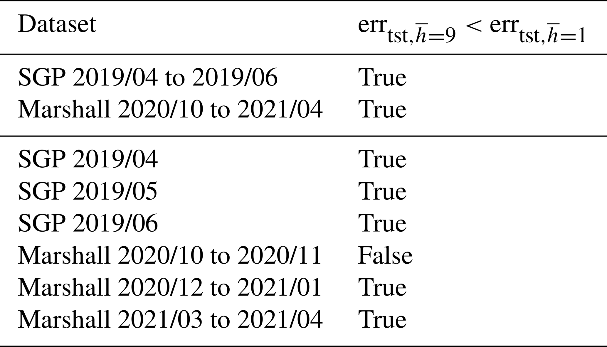
Table 6 shows that for five out of the six datasets the PTV-CF test errors are less than the PTV test error . The lower test errors of PTV-CF correlate with the higher WV accuracy that PTV-CF is able to achieve compared to PTV at the lower altitudes.
Table 6This table shows for which datasets the test error of the PTV-MPD method with the coarse-to-fine configuration is smaller (i.e., better) than PTV-MPD without the coarse-to-fine configuration . The first two rows of the table, before the horizontal divider line, correspond to the total test error comparison over all the SGP and Marshall datasets. The rest of the rows correspond to the test error comparison over the specific SGP and Marshall datasets.
PTV-MPD employs the photon-counting noise model to quantitatively fit the MPD forward models on the noisy observations, while encouraging accurate spatial and temporal correlations across all WV estimate pixels via the total variation regularizer function. This holistic approach allows for accurately measuring highly structured and varying WV fields at different altitudes and varying SNRs. In comparison, the standard method employs low-pass filters to reduce the residual noise in the WV estimate, and the low-pass filter bandwidth is optimized for lower-altitude (≤ 4 km) WV measurements. Therefore, the standard method, which uses high-altitude WV measurements, contains residual noise that degrades the measurements. By applying PTV-MPD to WV retrievals from the MPD, we have been able to extend the maximum altitude of the retrieval from 6 to 8 km, enabling a maximum coverage (after hardware improvements described in Spuler et al., 2021) from 150 m to 8 km by the instrument. In addition, the WV retrieval accuracy is substantially increased above 2 km. It is also notable that by employing the PTV-MPD method, the MPD WV measurement range extends beyond the that of the ARM-SGP Raman lidar, which has nearly 500 times the power-aperture product of the MPD (Newsom and Sivaraman, 2018).
We also demonstrated that without careful consideration of how PTV is adapted for the MPD instrument, low-altitude biases can be introduced in the PTV-MPD WV measurements. PTV-MPD requires an initial value of the attenuated backscatter, and any inaccuracies can induce biases in the PTV-MPD WV estimates. PTV-MPD can be made more robust against such biases by inferring the WV via a coarse-to-fine image resolution framework. By inferring the attenuated backscatter and WV at a coarse image resolution, inaccuracies in the initial attenuated backscatter are reduced, and subsequent finer image resolution attenuated backscatter estimates are more accurate, which allows for more accurate WV estimates.
As of now, PTV-MPD is computationally expensive since inferring the WV requires estimating the WV with several tuning parameters, and the optimal tuning parameter is selected through a cross-validation methodology. For example, with 144 CPU cores it takes 1 to 2 h to infer the WV using the PTV-MPD coarse-to-fine image resolution framework for 24 h of data; each CPU core estimates the WV for a specific tuning parameter. We are working towards developing a methodology to infer the optimal tuning parameter from the photon-counting observations, which will reduce the number of required CPU cores to 12 or less. In addition, adapting the PTV-MPD code to use a GPU instead of a CPU might reduce the computational time by at least 10-fold (Lee and Wright, 2008).
An additional benefit of decreasing the computational demands of PTV-MPD is that it would be able to process multiple days of consecutive observations and not just 24 h scenes as demonstrated in the results. A current workaround to process multiple-day scenes is to use a horizontal sliding window when inferring the WV. Specifically, the WV is inferred for consecutive overlapping 24 h periods, and the final multiple day WV image is obtained by averaging together the overlapping 24 h period WV estimates.
Future work includes the following goals.
-
The first is working towards quantifying the uncertainties of the PTV-MPD WV measurements using a bootstrapping methodology (Friedman et al., 2001). The uncertainty quantification will quantify how PTV-MPD WV measurements behave at the edges of scenes where less spatial information is available.
-
The second is investigating how PTV-MPD can be made more robust against saturated photon counts.
Define the indicator function as
The MPD forward model derivatives relative to WV and attenuated backscatter are
The P-NLL loss function derivatives relative to WV and attenuated backscatter are
Here we show that for high solar background radiation (i.e., lower SNR) of the photon-counting images there can be multiple estimates of the WV φ or attenuated backscatter that minimize the objective function (14). Specifically, we show that the P-NLL (8) has more the one minimizer. Without loss of generality we assume here that
-
the laser pulse duration is equal to the sampling intervals, meaning that ΔN=0 and the matrix A is just an identity matrix,
-
none of the photon counts are masked out by matrix M,
-
and p=1.
With these assumptions the Hessian matrix for observation column k of the P-NLL (8) relative to WV φ for given attenuated backscatter χ equals
If this Hessian matrix is positive definite, meaning all its eigenvalues are positive, then it implies that for a fixed attenuated backscatter χ there is a unique WV φ estimate that minimizes the P-NLL and therefore the objective function (14) (Boyd and Vandenberghe, 2004). The Hessian matrix is not positive definite if
Whether this inequality is met is dependent on the attenuated backscatter, WV transmittance, and laser energy. For example, for humid summer days the WV transmittance will significantly decrease the SSLE relative to the solar background radiation, consequently limiting PTV-MPD's ability to uniquely infer the WV at higher altitudes.
In the cases where the backscattered photons are comparable to the observed background counts according to Eq. (B4), we leave it to future work to determine the altitudes at which PTV-MPD can uniquely infer the WV.
The PTV-MPD code will be made available through a Git repository https://github.com/WillemMarais/poisson-total-variation (last access: 26 August 2022) in the near future.
All of the MPD data products used in this work were produced by NCAR and are available upon request; the raw MPD data are available at https://doi.org/10.26023/MX0D-Z722-M406 (NCAR/EOL MPD Team, 2020). The SGP radiosonde data are available via https://doi.org/10.5439/1373934 (ARM, 2022). The Marshall radiosonde data are available via the GCOS Reference Upper-Air Network (GRUAN) website https://www.gruan.org (last access: 26 August 2022, Hurst et al., 2022).
This work was a collaboration between the authors. WJM is the original developer of PTV and provided expertise in advanced signal processing. MH provided expertise in optical system modeling and DIAL observation. The PTV-MPD development was the result of a collaborative effort to mutually leverage the two disciplines.
The contact author has declared that none of the authors has any competing interests.
Publisher's note: Copernicus Publications remains neutral with regard to jurisdictional claims in published maps and institutional affiliations.
The authors would like to thank Robert A. Stillwell and Scott M. Spuler for their feedback on this paper. This material is based upon work supported by NSF AGS-1930907 and the National Center for Atmospheric Research, which is a major facility sponsored by the National Science Foundation under cooperative agreement no. 1852977. We thank Dale Hurst, Patrick Cullis, Emrys Hall, and Allen Jordan of the NOAA Global Monitoring Laboratory for providing the sounding data from the Marshall field site.
This research has been supported by the Division of Atmospheric and Geospace Sciences (grant no. NSF AGS-1930907) and the National Science Foundation (cooperative agreement no. 1852977). The MPD Net demo field campaign was supported by the Office of Biological and Environmental Research of the U.S. Department of Energy (under grant no. DOE/SC-ARM-20-002) as part of the Atmospheric Radiation Measurement (ARM) user facility, an Office of Science user facility.
This paper was edited by Hartwig Harder and reviewed by three anonymous referees.
Ahn, S. and Fessler, J.: Globally convergent image reconstruction for emission tomography using relaxed ordered subsets algorithms, IEEE T. Med. Imaging, 22, 613–626, https://doi.org/10.1109/TMI.2003.812251, 2003. a
ARM: Raman Lidar: Aerosol backscatter, scattering ratio, lidar ratio, extinction, cloud mask, and linear depolarization ratio derived from Thorson FEX code, ARM (Atmospheric Radiation Measurement) user facility [data set], https://doi.org/10.5439/1373934, 2022. a
Azzari, L. and Foi, A.: Variance stabilization in Poisson image deblurring, in: 2017 IEEE 14th International Symposium on Biomedical Imaging (ISBI 2017), 18–21 April 2017, Melbourne, VIC, Australia, 728–731, https://doi.org/10.1109/ISBI.2017.7950622, 2017. a, b
Beck, A. and Tetruashvili, L.: On the Convergence of Block Coordinate Descent Type Methods, SIAM J. Optimiz., 23, 2037–2060, https://doi.org/10.1137/120887679, 2013. a, b
Boyd, S. and Vandenberghe, L.: Convex optimization, Cambridge university press, ISBN 9780521833783, 2004. a
Cinlar, E.: Introduction to stochastic processes, Dover Publications, ISBN 9780486497976, 2013. a
Donovan, D. P., Whiteway, J. A., and Carswell, A. I.: Correction for nonlinear photon-counting effects in lidar systems, Appl. Opt., 32, 6742–6753, https://doi.org/10.1364/AO.32.006742, 1993. a, b
Fessler, J. A.: Optimization Methods for Magnetic Resonance Image Reconstruction: Key Models and Optimization Algorithms, IEEE Signal Proc. Mag., 37, 33–40, https://doi.org/10.1109/MSP.2019.2943645, 2020. a
Friedman, J., Hastie, T., and Tibshirani, R.: The elements of statistical learning, vol. 1, Springer series in statistics, New York, ISBN 0387848576, 2001. a, b, c
Geerts, B., Parsons, D., Ziegler, C. L., Weckwerth, T. M., Turner, D. D., Wurman, J., Kosiba, K., Rauber, R. M., McFarquhar, G. M., Parker, M. D., Schumacher, R. S., Coniglio, M. C., Haghi, K., Biggerstaff, M. I., Klein, P. M., Jr., W. A. G., Demoz, B. B., Knupp, K. R., Ferrare, R. A., Nehrir, A. R., Clark, R. D., Wang, X., Hanesiak, J. M., Pinto, J. O., and Moore, J. A.: The 2015 Plains Elevated Convection At Night (PECAN) field project, B. Am. Meteorol. Soc., 98, 767–786, https://doi.org/10.1175/BAMS-D-15-00257.1, 2016. a
Harmany, Z. T., Marcia, R. F., and Willett, R. M.: This is SPIRAL-TAP: Sparse Poisson Intensity Reconstruction ALgorithms – Theory and Practice, IEEE T. Image Process., 21, 1084–1096, https://doi.org/10.1109/TIP.2011.2168410, 2012. a, b, c, d, e, f, g, h
Hayman, M. and Spuler, S.: Demonstration of a diode-laser-based high spectral resolution lidar (HSRL) for quantitative profiling of clouds and aerosols, Opt. Express, 25, A1096–A1110, https://doi.org/10.1364/OE.25.0A1096, 2017. a, b
Hayman, M., Stillwell, R. A., and Spuler, S. M.: Optimization of linear signal processing in photon counting lidar using Poisson thinning, Opt. Lett., 45, 5213, https://doi.org/10.1364/OL.396498, 2020. a, b, c
Hurst, D., Cullis, P., Hall, E., and Jordan, A.: GCOS Reference Upper-Air Network (GRUAN), GRUAN Lead Centre, DWD, https://www.gruan.org, last access: 26 August 2022. a
Jensen, M. P., Petersen, W. A., Bansemer, A., Bharadwaj, N., Carey, L. D., Cecil, D. J., Collis, S. M., Genio, A. D. D., Dolan, B., Gerlach, J., Giangrande, S. E., Heymsfield, A., Heymsfield, G., Kollias, P., Lang, T. J., Nesbitt, S. W., Neumann, A., Poellot, M., Rutledge, S. A., Schwaller, M., Tokay, A., Williams, C. R., Wolff, D. B., Xie, S., and Zipser, E. J.: The Midlatitude Continental Convective Clouds Experiment (MC3E), B. Am. Meteorol. Soc., 97, 1667–1686, https://doi.org/10.1175/BAMS-D-14-00228.1, 2016. a
Kelley, C. T.: Iterative Methods for Optimization, Society for Industrial and Applied Mathematics, https://doi.org/10.1137/1.9781611970920, 1999. a
Lee, S. and Wright, S. J.: Implementing algorithms for signal and image reconstruction on graphical processing units, Optimization Online, 10, University of Wisconsin-Madison, https://optimization-online.org/2008/10/2131/ (last access: 2 September 2022), 2008. a
Marais, W. and Willett, R.: Proximal-Gradient methods for poisson image reconstruction with BM3D-Based regularization, in: 2017 IEEE 7th International Workshop on Computational Advances in Multi-Sensor Adaptive Processing (CAMSAP), 10–13 December 2017, Curacao, 1–5, https://doi.org/10.1109/CAMSAP.2017.8313128, 2017. a, b, c
Marais, W. J., Holz, R. E., Hu, Y. H., Kuehn, R. E., Eloranta, E. E., and Willett, R. M.: Approach to simultaneously denoise and invert backscatter and extinction from photon-limited atmospheric lidar observations, Appl. Opt., 55, 8316–8334, https://doi.org/10.1364/AO.55.008316, 2016. a, b, c, d, e, f, g
Müller, J. W.: Dead-time problems, Nucl. Instrum. Meth., 112, 47–57, https://doi.org/10.1016/0029-554X(73)90773-8, 1973. a
National Academies of Sciences, Engineering, and Medicine: The Future of Atmospheric Boundary Layer Observing, Understanding, and Modeling: Proceedings of a Workshop, The National Academies Press, Washington, DC, https://doi.org/10.17226/25138, 2018a. a
National Academies of Sciences, Engineering, and Medicine: Thriving on Our Changing Planet: A Decadal Strategy for Earth Observation from Space, The National Academies Press, Washington, DC, https://doi.org/10.17226/24938, 2018b. a
NCAR/EOL MPD Team: NCAR MPD data, Version 1.0, UCAR/NCAR – Earth Observing Laboratory [data set], https://doi.org/10.26023/MX0D-Z722-M406, 2020. a, b
Nehrir, A. R., Repasky, K. S., Carlsten, J. L., Obland, M. D., and Shaw, J. A.: Water Vapor Profiling Using a Widely Tunable, Amplified Diode-Laser-Based Differential Absorption Lidar (DIAL), J. Atmos. Ocean. Tech., 26, 733–745, https://doi.org/10.1175/2008JTECHA1201.1, 2009. a, b, c
Newsom, R. and Sivaraman, C.: Raman Lidar Water Vapor Mixing Ratio and Temperature Value-Added Products, Tech. rep., DOE Office of Science Atmospheric Radiation Measurement (ARM) Program (United States), https://doi.org/10.2172/1489497, 2018. a, b
NRC: Observing Weather and Climate from the Ground Up, National Academies Press, Washington, D.C., https://doi.org/10.17226/12540, 2009. a
NRC: When Weather Matters, National Academies Press, Washington, D.C., https://doi.org/10.17226/12888, 2010. a
NRC: Weather Services for the Nation, National Academies Press, Washington, D.C., https://doi.org/10.17226/13429, 2012. a
Oh, A. K., Harmany, Z. T., and Willett, R. M.: Logarithmic total variation regularization for cross-validation in photon-limited imaging, in: 2013 IEEE International Conference on Image Processing, 15–18 September 2013, Melbourne, VIC, Australia, 484–488, https://doi.org/10.1109/ICIP.2013.6738100, 2013. a, b, c, d, e, f, g
Oh, A. K., Harmany, Z. T., and Willett, R. M.: To e or not to e in poisson image reconstruction, in: 2014 IEEE International Conference on Image Processing (ICIP), 27–30 October 2014, Paris, France, 2829–2833, https://doi.org/10.1109/ICIP.2014.7025572, 2014. a
Roelofs, F., Janssen, M., Natarajan, I., et al.: SYMBA: An end-to-end VLBI synthetic data generation pipeline-Simulating Event Horizon Telescope observations of M 87, Astron. Astrophys., 636, A5, https://doi.org/10.1051/0004-6361/201936622, 2020. a
Schafer, R. W.: On the frequency-domain properties of Savitzky-Golay filters, in: 2011 Digital Signal Processing and Signal Processing Education Meeting (DSP/SPE), 4–7 January 2011, Sedona, AZ, USA, 54–59, https://doi.org/10.1109/DSP-SPE.2011.5739186, 2011. a
Spuler, S. M., Repasky, K. S., Morley, B., Moen, D., Hayman, M., and Nehrir, A. R.: Field-deployable diode-laser-based differential absorption lidar (DIAL) for profiling water vapor, Atmos. Meas. Tech., 8, 1073–1087, https://doi.org/10.5194/amt-8-1073-2015, 2015. a, b, c, d, e
Spuler, S. M., Hayman, M., Stillwell, R. A., Carnes, J., Bernatsky, T., and Repasky, K. S.: MicroPulse DIAL (MPD) – a diode-laser-based lidar architecture for quantitative atmospheric profiling, Atmos. Meas. Tech., 14, 4593–4616, https://doi.org/10.5194/amt-14-4593-2021, 2021. a, b, c, d, e, f, g, h
Weckwerth, T. M., Wulfmeyer, V., Wakimoto, R. M., Hardesty, M. R., Wilson, J. W., and Banta, R. M.: NCAR-NOAA Lower-Tropospheric Water Vapor Workshop, B. Am. Meteorol. Soc., 80, 2339–2357, https://doi.org/10.1175/1520-0477(1999)080<2331:WOTOFE>2.0.CO;2, 1999. a
Willett, R. and Nowak, R.: Platelets: a multiscale approach for recovering edges and surfaces in photon-limited medical imaging, IEEE T. Med. Imaging, 22, 332–350, https://doi.org/10.1109/TMI.2003.809622, 2003. a
Wulfmeyer, V., Hardesty, R. M., Turner, D. D., Behrendt, A., Cadeddu, M. P., Di Girolamo, P., Schlüssel, P., Van Baelen, J., and Zus, F.: A review of the remote sensing of lower tropospheric thermodynamic profiles and its indispensable role for the understanding and the simulation of water and energy cycles, Rev. Geophys., 53, 819–895, https://doi.org/10.1002/2014RG000476, 2015. a
Xiao, D., Wang, N., Shen, X., Landulfo, E., Zhong, T., and Liu, D.: Development of ZJU High-Spectral-Resolution Lidar for Aerosol and Cloud: Extinction Retrieval, Remote Sens., 12, 3047, https://doi.org/10.3390/rs12183047, 2020. a, b
Information about the project is available at https://www.arm.gov/research/campaigns/sgp2019mpddemo (last access: 26 August 2022).
- Abstract
- Introduction
- The MPD forward models
- The MPD photon-counting noise model and masking
- The MPD standard method
- The PTV-MPD method
- Experiment results
- Conclusion and future work
- Appendix A: Jacobian matrix of MPD forward models (Eq. 5) and gradient matrix of loss function (Eq. 12)
- Appendix B: Poisson negative log likelihood Eq. 8 properties
- Code availability
- Data availability
- Author contributions
- Competing interests
- Disclaimer
- Acknowledgements
- Financial support
- Review statement
- References