the Creative Commons Attribution 4.0 License.
the Creative Commons Attribution 4.0 License.
 | 21 Sep 2022
Identifying cloud droplets beyond lidar attenuation from vertically pointing cloud radar observations using artificial neural networks
Willi Schimmel
Heike Kalesse-Los
Maximilian Maahn
Teresa Vogl
Andreas Foth
Pablo Saavedra Garfias
Patric Seifert
In mixed-phase clouds, the variable mass ratio between liquid water and ice as well as the spatial distribution within the cloud plays an important role in cloud lifetime, precipitation processes, and the radiation budget. Data sets of vertically pointing Doppler cloud radars and lidars provide insights into cloud properties at high temporal and spatial resolution. Cloud radars are able to penetrate multiple liquid layers and can potentially be used to expand the identification of cloud phase to the entire vertical column beyond the lidar signal attenuation height, by exploiting morphological features in cloud radar Doppler spectra that relate to the existence of supercooled liquid. We present VOODOO (reVealing supercOOled liquiD beyOnd lidar attenuatiOn), a retrieval based on deep convolutional neural networks (CNNs) mapping radar Doppler spectra to the probability of the presence of cloud droplets (CD). The training of the CNN was realized using the Cloudnet processing suite as supervisor. Once trained, VOODOO yields the probability for CD directly at Cloudnet grid resolution. Long-term predictions of 18 months in total from two mid-latitudinal locations, i.e., Punta Arenas, Chile (53.1∘ S, 70.9∘ W), in the Southern Hemisphere and Leipzig, Germany (51.3∘ N, 12.4∘ E), in the Northern Hemisphere, are evaluated. Temporal and spatial agreement in cloud-droplet-bearing pixels is found for the Cloudnet classification to the VOODOO prediction. Two suitable case studies were selected, where stratiform, multi-layer, and deep mixed-phase clouds were observed. Performance analysis of VOODOO via classification-evaluating metrics reveals precision > 0.7, recall ≈ 0.7, and accuracy ≈ 0.8. Additionally, independent measurements of liquid water path (LWP) retrieved by a collocated microwave radiometer (MWR) are correlated to the adiabatic LWP, which is estimated using the temporal and spatial locations of cloud droplets from VOODOO and Cloudnet in connection with a cloud parcel model. This comparison resulted in stronger correlation for VOODOO (≈ 0.45) compared to Cloudnet (≈ 0.22) and indicates the availability of VOODOO to identify CD beyond lidar attenuation. Furthermore, the long-term statistics for 18 months of observations are presented, analyzing the performance as a function of MWR–LWP and confirming VOODOO's ability to identify cloud droplets reliably for clouds with LWP > 100 g m−2. The influence of turbulence on the predictive performance of VOODOO was also analyzed and found to be minor. A synergy of the novel approach VOODOO and Cloudnet would complement each other perfectly and is planned to be incorporated into the Cloudnet algorithm chain in the near future.
- Article
(10295 KB) - Full-text XML
- BibTeX
- EndNote


In mixed-phase clouds, the variable mass ratio between liquid water and ice as well as its spatial distribution within the cloud plays an important role in cloud lifetime (Morrison et al., 2012), precipitation processes (Mülmenstädt et al., 2015), climate feedbacks (Choi et al., 2014; Bjordal et al., 2020), and the radiation budget (Sun and Shine, 1994; Shupe et al., 2004; Turner, 2005). Modeling mixed-phase clouds is challenging and requires the basic assumption of thermodynamic phase, i.e., ice, liquid, or mixed (Zhao et al., 2012). Improving methods for cloud phase classification is a first step towards minimizing the error of liquid water content (LWC) and particle size retrievals (Riihimaki et al., 2016). Accurately observing the phase distribution within mixed-phase clouds has historically been one of the major challenges for the remote sensing community (Shupe et al., 2008). Multisensor retrievals rely mostly on valid lidar signals (Shupe et al., 2005; Illingworth et al., 2007; de Boer et al., 2009; Silber et al., 2020) in synergy with Doppler cloud radar moments, limiting the liquid classification due to lidar attenuation (Shupe et al., 2004; Sokol et al., 2018). The lidar signal is strongly attenuated by liquid water layers with optical depths τ ∼ 3–5 (Silber et al., 2020), hampering the use of lidar-based hydrometeor target classification for optically thick clouds. Radars are able to penetrate multiple liquid layers and can thus be used to expand the identification of cloud phase to the entire vertical column beyond the lidar signal attenuation height, if morphological features in cloud radar Doppler spectra can be related to the existence of supercooled liquid droplets.
Several efforts have been made in the past to exploit these features and derive the distribution of liquid in mixed-phase clouds: continuous-wavelet transformations in combination with fuzzy logic using fixed thresholds to identify liquid peaks in simulated Doppler spectra have been employed by Yu et al. (2014). Doppler spectra peak-finding algorithms like PEAKO (Kalesse et al., 2019; a supervised learning method) and peakTree (Radenz et al., 2019; a binary tree approach) can be used to identify the number of radar Doppler spectra peaks at each time–height step. In the next step, individual peaks can be related to liquid droplet existence based on the sub-peak radar moment analysis as done in Radenz et al. (2019). Silber et al. (2020) applied statistical tests to cumulative distribution functions and probability density functions of radar moments and temperature measurements by soundings to discriminate liquid-bearing from pure-ice cloud layers. Kalogeras et al. (2021) presented another method that used climatologically derived, per-phase probability distributions to retrieve an ice–liquid partitioning via a per-pixel, neighborhood-dependent algorithm. Also, deep learning approaches have been used in the past to derive a liquid mask from lidar backscatter coefficient and depolarization predicted from Doppler radar spectra (Luke et al., 2010). Although the applicability of machine learning to cloud radar data has been demonstrated by Luke et al. (2008, 2010) and Kalesse et al. (2019), its potential is far from being fully exploited. The aim is to develop a robust method which is able to directly relate raw Doppler spectra information to the presence of liquid hydrometeors, without the need for complex feature engineering and extraction.
The interest in machine learning and particularly deep learning in the Earth system sciences has strongly increased in the past few years (Maskey et al., 2020). Deep learning techniques are a subset of machine learning, where deep artificial neural networks (ANNs) learn relationships from data. These applications are particularly powerful due to their ability to perform part of the data pre-processing themselves. Vogl et al. (2022) showed that ANNs can be used to predict riming using ground-based zenith-pointing cloud radar variables radar reflectivity, spectrum width, and skewness. An earlier approach from Luke et al. (2010) transfers the features of Doppler spectra into particle backscatter and volume depolarization of a high-spectral-resolution lidar (HSRL) using a multi-layer perceptron model and was further validated by Kalesse-Los et al. (2022) by applying the pre-trained machine learning model to data from the Analysis of the Composition of Clouds with Extended Polarization Techniques (ACCEPT) campaign (Myagkov et al., 2016a, b). The methods mentioned above rely mostly on fixed thresholds for radars (i.e., reflectivity, mean Doppler velocity, spectrum width, skewness, spectrum edge slopes) and lidars (i.e., attenuated backscatter and depolarization) and are only applicable for a small subset of cloud types (Luke et al., 2008, 2010; Yu et al., 2014; Kalesse et al., 2019; Silber et al., 2020). Nevertheless, in the study of Kalesse-Los et al. (2022), the Luke et al. (2010) model displayed the ability to perform well on Doppler spectra recorded by a different cloud radar in different atmospheric conditions.
In this study we build upon the idea of Luke et al. (2010) and use a deep convolutional neural network (CNN) model to directly predict a probability of the distribution of supercooled cloud droplets in mixed-phase clouds observed by a vertically pointing Doppler cloud radar. Relevant spectral signatures such as bi-modalities, spectral skewness, and temporal evolution can be extracted by a deep CNN that relates to the cloud phase by training in a supervised scheme, using Cloudnet's target classification as supervisor. As part of the pan-European Aerosol, Clouds and Trace Gases Research Infrastructure (ACTRIS), the Cloudnet processing suite (Illingworth et al., 2007; Tukiainen et al., 2020a) is tailored to process observations and model data on the composition of the atmosphere. The measurements and model data are brought on a common grid, and the targets are classified as ice, liquid, aerosol, and insects, among others. Here, the information about the presence of liquid droplets is extracted from the Cloudnet target classification and in a first step used to train VOODOO. In the next step, Cloudnet data which were not used for training are compared to the predictions of VOODOO. Various binary classification metrics are used to quantify performance, such as precision, recall, accuracy, and F1 score. Further evaluation is done by correlating several independent measurements such as liquid water path (LWP) retrieved by microwave radiometer as suggested by Luke et al. (2010) and Kalesse-Los et al. (2022).
The paper is structured as follows. Section 2 gives an overview about the instrumentation and the data sets used in the context of this work. In Sect. 3 the methodology of the VOODOO retrieval is presented. Section 4 is divided into the analysis of a case study and the statistical evaluation of VOODOO by application to a total of 18 months of measurement data from two different geographical locations. The paper concludes with a summary and outlook in Sect. 5.
This section introduces the instrumentation used to train and validate the CNN performance. First, the data sources are presented (Sect. 2.1), followed by a short description of the two field experiments in Punta Arenas and Leipzig, including specifics of the respective sites (Sect. 2.2).
2.1 Data source
Four data sources (see Table 1) are considered for the presented CNN retrieval: cloud radar Doppler spectra from a vertically pointing radar, attenuated backscatter coefficient βatt from a ceilometer, liquid water path (LWP) retrieved from a microwave radiometer (MWR), and temperature, relative humidity, and pressure from numerical weather forecast data from the European Centre for Medium-Range Weather Forecasts (ECMWF).
(Küchler et al., 2017)(Rose et al., 2005)(Heese et al., 2010)(Owens and Hewson, 2018)Table 1Specifications of instruments/models and measured/modeled quantities used in this study.

Doppler cloud radars record the distribution of reflectivity in the Doppler velocity domain continuously in time and provide vertically resolved observations with excellent sensitivity to small hydrometeors (Kollias et al., 2007). Figure 1 shows hydrometeors creating peaks at distinct terminal fall velocities in the Doppler radar spectra; the larger and heavier they are, the faster they fall (assuming no vertical air motion). The radar reflectivity factor Ze in the Rayleigh scattering regime is sensitive to the sixth power of the diameter, , where N is the number of hydrometeors for diameter D. It follows that Ze is larger for small populations of large hydrometeors such as ice crystals or drizzle and rain, thus dominating the spectral signal by producing large peaks at higher fall velocities. In contrast, cloud droplets exist in the atmosphere with much larger N but much smaller D at ≈ 0 m s−1 terminal velocity, producing low-intensity peaks in the Doppler spectra. The radar moments, i.e., reflectivity factor Ze, mean Doppler velocity , and spectral width σw, and linear depolarization ratio (LDR) are computed from the Doppler spectra. These radar moments are required for Cloudnet processing and are usually sufficient to derive a mask for precipitation and ice crystals (Illingworth et al., 2007). However, these radar moments alone are not sufficient in all situations to provide the necessary information content to characterize liquid and mixed-phase clouds reliably.
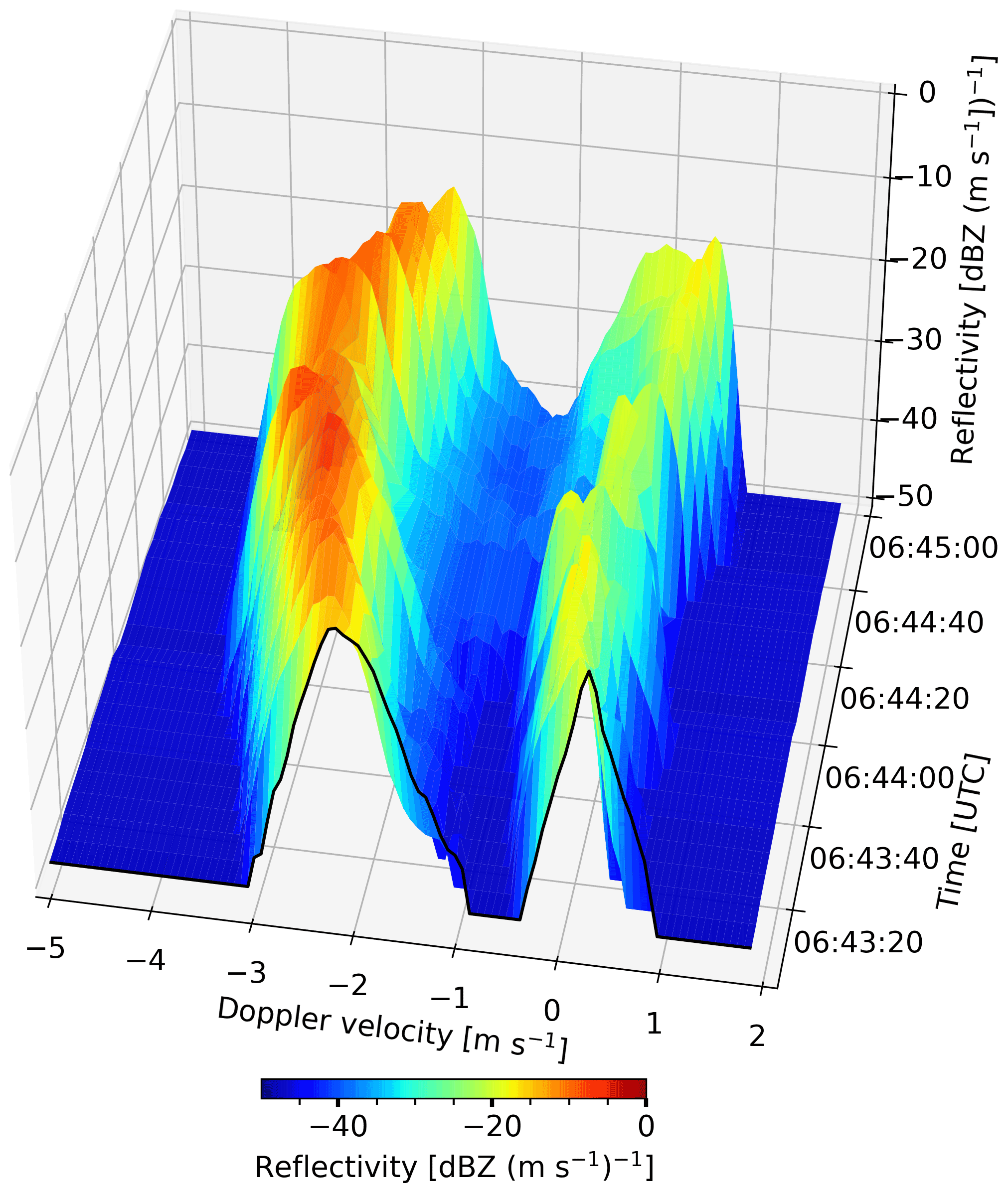
Figure 1Time spectrogram from 1 August 2019 at 2400 m altitude in Punta Arenas, Chile. The bi-modal Doppler spectra contain liquid cloud droplets on the right-hand side of the spectrum (slow moving) and ice crystals on the left side of the spectrum (faster moving). Cloudnet classification result for this particular time-range slice is “ice and supercooled liquid droplets” at −10 ∘C.
The ceilometer provides high-resolution profiles of attenuated backscatter coefficient βatt at 1064 nm. The parameter βatt is sensitive to the second power of the diameter, . It follows that βatt is larger for large populations of small hydrometeors (cloud droplets). Small numbers of larger ice crystals, drizzle, or raindrops return a much lower signal. Due to its very high sensitivity to cloud droplets, βatt is used in the Cloudnet processing to identify cloud droplets.
The MWR measures brightness temperature profiles over a band of different frequencies. To derive the LWP and integrated water vapor (IWV), optimal estimation (Foth and Pospichal, 2017) or artificial neural network retrievals (Yan et al., 2020, or MWR manufacturer) are used. The LWP is a measure for the amount of liquid water in the column above the instrument and used for validation purposes in the frame of this work. The MWR–LWP is correlated to the LWP derived from VOODOO predictions using an adiabatic cloud parcel model by Karstens et al. (1994), as illustrated in Kalesse-Los et al. (2022).
Temperature, relative humidity, and pressure profiles, taken from the European Centre for Medium-Range Weather Forecasts (ECMWF) model, are used in combination with MWR–LWP to derive atmospheric profiles of gaseous and liquid attenuation for correction of the radar returns used within the Cloudnet processing chain. The numerical weather forecast data can be downloaded via the Cloudnet data portal (https://cloudnet.fmi.fi, last access: 12 September 2022).
2.2 Data sets from Punta Arenas and Leipzig
This work is based on remote sensing measurements from two different geographical locations, i.e., Punta Arenas, Chile, and Leipzig, Germany. Selected key properties of the two sites are summarized in Table 2. First, observations from the long-term field experiment Dynamics, Aerosol, Cloud, and Precipitation Observations in the Pristine Environment of the Southern Ocean (DACAPO-PESO) in Punta Arenas, Chile, are discussed, and second, observations from the roof platform of the main building of the Leipzig Institute of Meteorology in Leipzig (LIM), Germany, are analyzed.
Kanitz et al. (2011)Ansmann et al. (2005)Ohneiser et al. (2020)Seifert et al. (2010)Bromwich et al. (2020)Bühl et al. (2013)Jimenez et al. (2020)Bühl et al. (2016)Floutsi et al. (2021)Radenz et al. (2021)Radenz et al. (2021)Vogl et al. (2022)Vogl et al. (2022)Table 2Overview on location, data availability, climate, aerosol load, and related studies for the data sets used. The altitudes are given above mean sea level (a.s.l.).
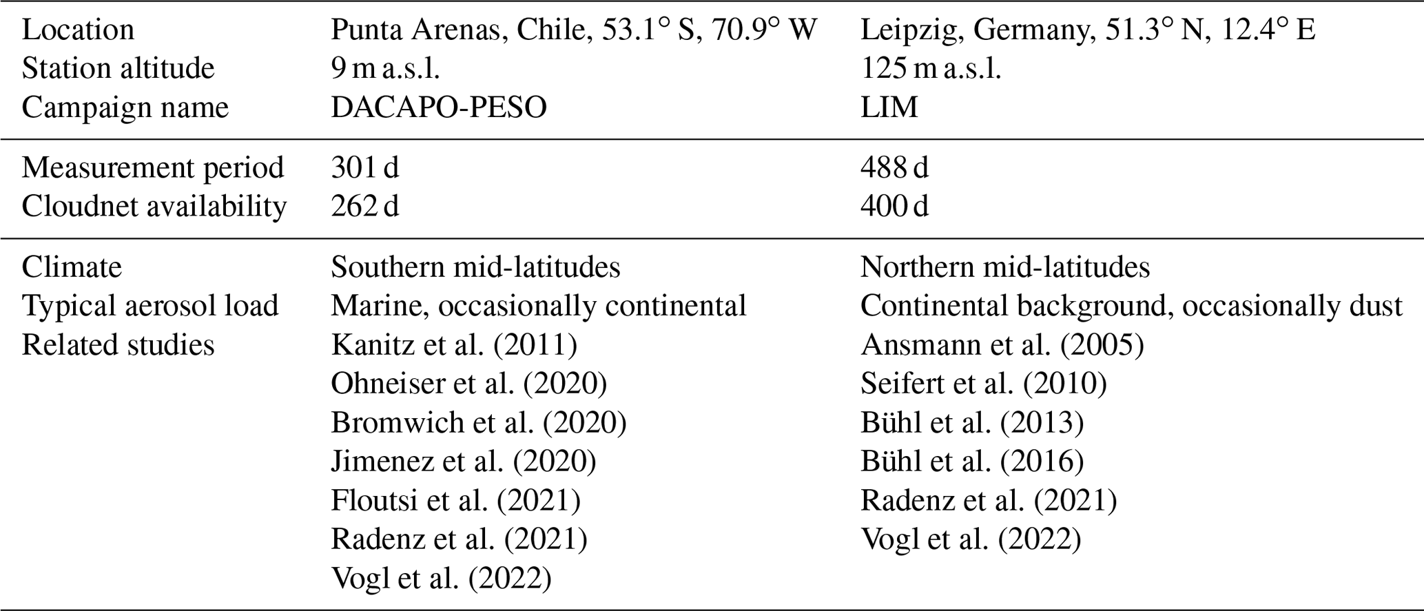
DACAPO-PESO focuses on the investigation of aerosol–cloud dynamics and interactions in the atmosphere. A unique data set has been gathered by synergistic retrievals with active and passive remote sensors. Clean pristine marine air masses dominate the aerosol conditions, due to almost constant westerly winds (Schneider et al., 2003; Foth et al., 2019; Jimenez et al., 2020; Floutsi et al., 2021; Radenz et al., 2021). Additionally, gravity waves have been observed frequently over Punta Arenas (Alexander et al., 2017; Silber et al., 2020; Radenz et al., 2021). Due to orographic effects induced by strong westerly winds moving over the Andes mountain range, gravity waves are a general feature in the vicinity of all landmasses in the middle and high latitudes of the Southern Hemisphere (Sato et al., 2012; Alexander et al., 2016). The Leipzig Aerosol and Cloud Remote Observations System (LACROS) suite has been deployed by the Leibniz Institute for Tropospheric Research (TROPOS) from 27 November 2018 to 20 November 2021. LIM contributed a RPG-FMCW94 Doppler cloud radar, operating from 27 November 2018 until 27 September 2019, to enhance the information content of the DACAPO-PESO field campaign.
The second data set includes measurements recorded at the roof platform of the main building of the Leipzig Institute of Meteorology (LIM). The observations included in this work were conducted from 17 December 2020 to 6 March 2022. Leipzig is located in central Europe and is predominantly influenced by continental air masses, anthropogenic pollution (Baars et al., 2016), and occasional mineral dust events (Seifert et al., 2010). A more in-depth analysis of aerosol contributions for both sites can be found in Radenz et al. (2021).
This section introduces the machine learning methodology used to derive a spatio-temporal liquid cloud droplet probability distribution directly from spectra of the vertically pointing Doppler cloud radar. A CNN is trained on radar Doppler spectra using the atmospheric target classification retrieved by the Cloudnet algorithm (Illingworth et al., 2007; Tukiainen et al., 2020a) as supervisor. An example is given in Fig. 2. Firstly, the pre-processing of Doppler radar spectra and sampling of features is presented in Sect. 3.1. Secondly, Cloudnet processing is done to derive the hydrometeor target classification reference labels for the training data, explained in Sect. 3.2. Section 3.3 describes the machine learning model, followed by introducing the training and validation data sets in Sect. 3.4. Information about the training process is given in Sect. 3.5. Post-processing steps are described in Sect. 3.6, and validation metrics are presented in Sect. 3.7.
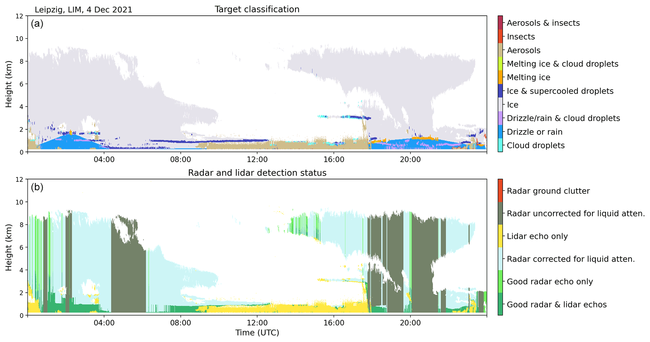
Figure 2Cloudnet target classification (a) and radar–lidar detection status (b) for 4 December 2021 in Leipzig, Germany.
3.1 Pre-processing and feature sampling
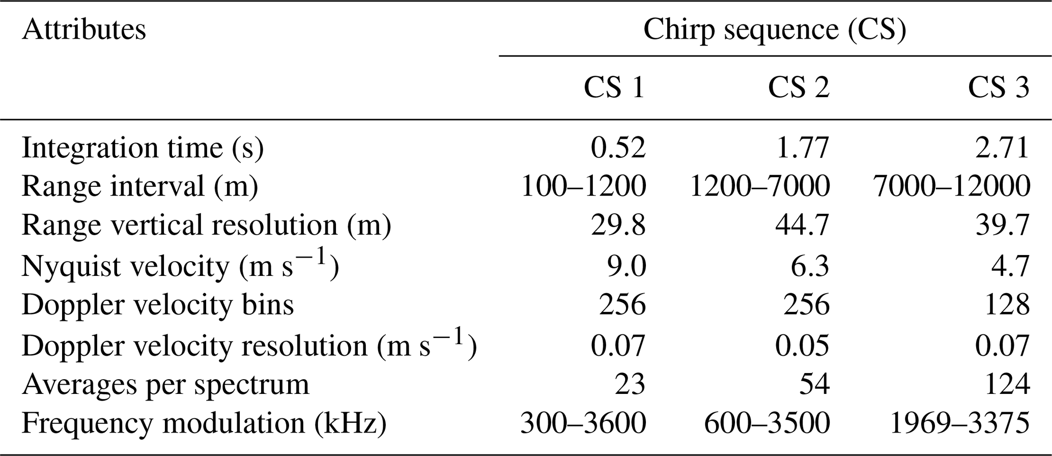
Firstly, the raw radar Doppler spectra are pre-processed as follows. The RPG-FMCW-94-DP radar operates with different settings, through a user-defined measurement definition file. Table 3 contains the instrument settings which were identical for both sites. By modulating the center frequency (94 GHz) in ranges of 300–3600 kHz, the atmosphere is sampled consecutively by three programs (chirps) collecting Doppler radar spectra for the three ranges of operation or chirp sequences (CSs) consecutively. Each CS has slightly different range and Doppler velocity resolution, as well as different Nyquist velocity vNyq, number of Doppler spectra bins, frequency modulation ranges, and number averages (coherently and non-coherently) for a single spectrum (see Table 3).
Table 3Specifications and program settings for the vertically pointing RPG-FMCW-94-DP Doppler cloud radar.
The pre-processing steps listed below are split into general pre-processing necessary to obtain the Cloudnet products and spectral feature extraction.
-
Received vertical and horizontal polarized signals are summed, yielding the total back-scattered signal intensity.
-
Noise in the Doppler radar spectra is estimated and removed via manufacturer software, which uses the method of Hildebrand and Sekhon (1974). The cut-off threshold for noise removal is set at mean noise power plus 6 standard deviations of the noise power.
-
The radar moments Ze, , σw, and LDR are estimated from the spectra and stored as NetCDF files. Those files are used as input for the Cloudnet processing.
-
The Cloudnet target classification is derived (see Sect. 3.2).
Spectral feature extraction is done by adjusting the radar Doppler spectra for VOODOO processing.
-
The presented method is designed for Doppler radar spectra counting 256 Doppler velocity bins. If the number of Doppler velocity bins does not match 256, nearest-neighbor interpolation is applied to meet the number of 256 Doppler bins.
-
Doppler bins which were removed from the Doppler spectra by noise filtering are replaced by their range-dependent sensitivity limit, also provided by the RPG software.
-
The radar Doppler spectra are then converted from linear units mm6 m−3 into units of dBZ via
where S(vD) is the spectral power as a function of velocity vD.
-
The radar Doppler spectra are normalized by
where dBZ and dBZ are the maximum and minimum expected values. S(vD) values above and below this range are set to the corresponding Smax and Smin, respectively.
-
Successively recorded spectra Ns for each range gate are combined to form a time spectrogram , with s and ti being a time step on the temporal domain of the Cloudnet products. Using the radar settings from Table 3, i.e., 5 s temporal resolution, the number of successively recorded spectra used is Ns=6. The grid size of Cloudnet is used as target, i.e., 30 s temporal resolution and range resolution between 30–45 m, depending on the respective chirp.
-
The corresponding labels are assigned: cloud droplets present (i.e., Cloudnet classes: liquid and mixed-phase clouds) and no cloud droplets present (i.e., Cloudnet classes: ice, insects, drizzle, and rain). Finally, a list of time spectrograms X and their corresponding labels y is generated.
Figure 1 shows an exemplary feature sample (time spectrogram), where a fast-falling population of large ice crystals is visible as a peak at −3 m s−1and high spectral reflectivity of up to −8 dBZ. The second peak at ≈ 0 m s−1 indicates a population of supercooled liquid cloud droplets ( ∘C) with reflectivity values up to −18 dBZ.
3.2 Cloudnet target classification as reference label
Supervised deep learning approaches require large numbers of pairs of input (features) and output (labels) to learn from. For this work, the Cloudnet target classification provided by the Cloudnet processing toolbox (Tukiainen et al., 2020a) is used to generate the reference label. In the first step radar moments, (i.e., Ze, , σw, and LDR) are calculated from the recorded Doppler radar spectra. Radar moments together with ceilometer βatt, MWR–LWP, precipitation rate (from Vaisala WXT536 compact weather station mounted to the cloud radar), and meteorological data are processed using the Cloudnet algorithm to derive an a priori hydrometeor target classification. Cloudnet provides two bit masks, the category-bit, containing information on the nature of the targets for each data point (i.e., droplets present, is falling, insects) and the quality-bit, which contains information on the instrument detection status (i.e., echo detected by radar, echo detected by lidar). The combination of active bits yield the Cloudnet target classification and detection status (see Fig. 2). The Cloudnet liquid droplet detection investigates the shape of the ceilometer attenuated backscatter coefficient profile βatt and the attenuation height above the liquid layer base (Tuononen et al., 2019). At an approximate optical thickness of τ>3 the lidar is completely attenuated such that hydrometeor thermodynamic phase information above the attenuation height is unreliable. The top panel of Fig. 2 displays such attenuation effects in the mixed-phase layer within a convective system from 04:00 to 06:30 UTC. The lidar attenuation height of 250 m is indicated by the detection status “Radar uncorrected for liquid attenuation” in Fig. 2 (bottom). Thus, the training data set is automatically selected by unifying all data points where liquid cloud droplets are present (Cloudnet liquid category bit) and where the detection status indicates both good radar and lidar echoes. This technique avoids manual labeling. By default, Cloudnet corrects the lidar-detected liquid cloud depth using radar data, by extending a liquid layer to cloud top if the detected cloud top by radar was less than 500 m above the liquid layer base, even though no clear sign of liquid is given due to the attenuation of the lidar signal. Here, to minimize the number of falsely classified liquid-containing data points, this liquid extension to cloud top was disabled.
3.3 Architecture of the machine learning model
The following section introduces the machine learning model used to relate Doppler spectra morphologies to the presence of liquid cloud droplets. The output of VOODOO is a probability distribution over a discrete set of two classes, i.e., “cloud droplets present” and “other targets”. The machine learning approach utilizes ideas from computer vision by means of image classification via a CNN (LeCun et al., 1989; Krizhevsky et al., 2012). These methods learn the complex structure in large data sets by using optimization strategies such as gradient descent variants (Ruder, 2016) in combination with backpropagation (Kelley, 1960; Hecht-Nielsen, 1989) for optimizing the internal parameters. The aim is to find a set of parameters that minimizes the error for predictions.
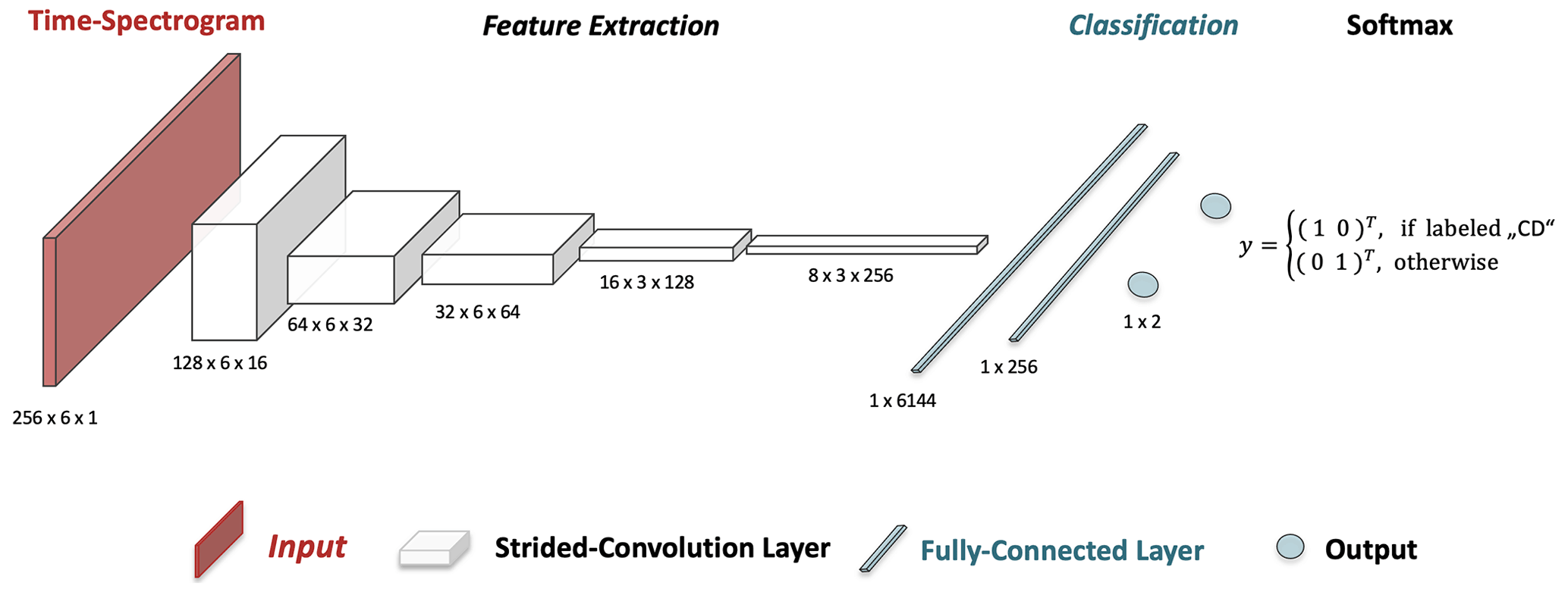
Figure 3Illustration of the CNN architecture. The time spectrogram serves as input to the VOODOO model. Five feature extraction layers follow the input layer performing strided-convolution operations. While the number of features which can be extracted increases from 16 to 256, the size of the feature maps shrinks from 128 by 6 to 8 by 3 pixels. The feature extraction is followed by two fully connected layers with and 256 nodes. The output is a vector with two elements, with .
A CNN classifier, implemented in PyTorch (Paszke et al., 2019), is trained on cloud radar Doppler spectra morphologies to relate to the availability of liquid cloud droplets. Figure 3 shows the architecture of the VOODOO retrieval algorithm, which is split into a feature extraction segment consisting of multiple convolutional layers and a classification segment consisting of two fully connected layers. Information such as signal intensity, shape, temporal evolution, location of peaks, and other morphological features of Doppler spectra can be extracted by convolution layers. CNNs (LeCun et al., 1989; Goodfellow et al., 2013; LeCun et al., 2015; Goodfellow et al., 2016) are a specialized kind of neural network for processing data that has a known, grid-like topology like a 2D grid of data points, i.e., the time spectrogram. Using the terminology of Goodfellow et al. (2016, p. 330), each of the convolution layers in Fig. 3 are comprised of multiple stages: stride convolution (affine transformation) and detector stage (non-linear activation function). The 2D convolution operation extracts local features by convolving trainable 2D filters (kernels) with the input, along the velocity–time axis (x–y axis). During the convolution operation the kernels are shifted by two data points along the velocity axis (x axis), called stride (Springenberg et al., 2014), to merge semantically similar features into one, hence reducing the size of the previous layer by a factor of 2 in each layer. Additionally, the third convolutional layer shifts the feature map by two data points along the time axis (y axis). As the number of extractable features increases from 16 to 256 per layer, the spatial dimension decreases from (256, 6) to (8, 3); thus the precise location of features gets less relevant in deeper layers. The last convolutional layer is followed by two fully connected layers which compute non-linear input–output mappings from the extracted 2D features. To add non-linearity to the CNN model, the linear transformation (matrix–vector product) in each layer is applied to a non-linear activation function. The exponential linear unit (ELU) used for all hidden layers is a smooth continuous function and easy to differentiate. ELU is defined as follows:
with default α=1.0 and . The softmax function in the last layer provides a probability for the prediction of the discrete set of two classes.
Finally, the threshold p∗ controls the classification into cloud droplets present (CD) if and cloud droplets not present (noCD) if . This parameter p∗ can be manually adjusted by the user or computed automatically by receiver operating characteristics, i.e., ROC-curve analysis (Zou et al., 2007). Note that the output of the network should not be interpreted as a probability density function, which represents a notion of confidence. Instead it is a pseudo probability or likelihood for each class. For better readability the term “pseudo” is omitted subsequently.
3.4 Training and validation set
The presented machine leaning technique is trained on 10 % of DACAPO-PESO (Punta Arenas) data measured by the RPG-FMCW-94-DP Doppler cloud radar. While larger training sets usually increase the performance in deep learning models, no major advantages could be observed, when more than 10 % of the available data set was used for training. The remaining 90 % of data from Punta Arenas and 100 % of data obtained in Leipzig are used to validate the predictive performance. For Leipzig, a list of 50 d was removed from the entire data set, by filtering out days with clear sky only, the sole presence of very thin clouds with LWP below 20 g m−2, precipitation lasting all day, artifacts in the radar spectra from a nearby construction crane, and ceilometer observations that are fully attenuated below 200 m. Isolated data points (speckles) are removed from the data set. Finally, the outer three data points along the edge of each observed cloud were omitted from the training and validation data set, to reduce the effects of partial beam filling (radar sample volume partially filled with atmospheric targets).
3.5 Training process
During training, VOODOO is fed by a time spectrogram and outputs a vector of scores, one for each category. An objective function measures the error (or loss) between the output and the desired target. Via a modified stochastic gradient descent, the categorical cross-entropy loss function
is minimized, where and is the predicted pseudo-probability for class j, and , where , represents the one-hot-encoded labels (see Sect. 3.1). One-hot encoding is used to convert the categorical data (labels) to numerical data required by machine learning algorithms. To reduce the loss function J, the internal hyperparameters (kernels and fully connected layer weights) are adjusted by applying the adaptive moment estimation (Adam) optimization method (Kingma and Ba, 2017), which uses a stochastic gradient-based optimization approach. Gradient descent (Ruder, 2016) in combination with backpropagation (Kelley, 1960; Hecht-Nielsen, 1989) adjusts the hyperparameters iteratively to minimize J. Processing was done on a GPU workstation using four NVIDIA RTX 8000 instruments. Training 10 epochs takes approximately 15 min. However, the optimization plateaus already after three epochs. The term epoch refers to one cycle through the full training data set and can also be considered the iteration of optimization.
3.6 Post-processing
In the last step, the raw VOODOO predictions L (Eq. 4) are assigned to the original coordinates in the spatio-temporal domain and convolved with the two-dimensional Gaussian filter
where x and y correspond to the time and range indices, respectively, and σ=1, to generate more coherent structures. After classification into no cloud droplets present and cloud droplets present using the p∗ threshold (see Sect. 3.3), all data points with mean Doppler velocity below −3 m s−1 are re-classified as no cloud droplets present. This value gives a good compromise between physically reasonable (drizzle and rain correspond to faster-falling hydrometeors) and the influence of gravity waves, the latter being omni-present in Punta Arenas (Radenz et al., 2021).
3.7 Performance validation
This section lists common measures for validation of the predictive performance of VOODOO. In the following, “CD” refers to cloud droplets present samples (i.e., the positive class) and “noCD” to cloud droplets not present samples (i.e., the negative class). The confusion matrix C(p∗) summarizes all counts of the correct and misclassified data samples for each class. This two-by-two matrix consists of the numbers of correctly identified CD (true positives, TP, hits) and noCD (true negative, TN) samples on the main diagonal of the matrix, as well as falsely classified noCD (false positive, FP, false alarm) and CD (false negative, FN, misses) samples on the off-diagonal, i.e.,
The value of p∗, i.e., the probability threshold necessary for classification as CD (see Sect. 3.3), is adjustable and controls the ratio of false positive and false negative predictions. Increasing p∗ increases the number of false negatives and decreases the number of false positives. Vice versa is true, if p∗ is decreased. The thresholds were selected manually after investigating the ROC curve (Zou et al., 2007), yielding good balance between misses (FN) and false alarms (FP). The listing below gives the performance scores used to evaluate the retrieval, similar to Kalesse-Los et al. (2022).
-
Precision or positive predictive value (PPV) is a real value between 0 and 1, where 1 is the perfect score.
i.e., the fraction of how many predictions where correctly classified as CD (i.e., TP) and the sum of TP and predictions falsely classified as CD (i.e., FP). In the context of this work, it measures the amount of CD overestimation.
-
Negative predictive value (NPV) is a real value between 0 and 1, where 1 is the perfect score.
i.e., the fraction of how many noCD predictions where correctly classified as such (i.e., TN) and the sum of TN and predictions falsely classified as noCD (i.e., FN). In the context of this work, it measures the number of correctly identified noCD samples.
-
The recall or true positive rate (TPR) is a real value between 0 and 1, where 1 is the perfect score.
i.e., the fraction of TP and the sum of TP and liquid-containing pixels, which were falsely classified as noCD (i.e., FN). In the context of this work, recall measures the amount of CD underestimation. The closer recall gets to 1, the less likely it is missing an actual CD.
-
Selectivity or true negative rate (TNR) is a real value between 0 and 1, where 1 is the perfect score.
i.e., the fraction of TN and the sum of TN and noCD samples, which were falsely classified as CD (i.e., FP). As selectivity approaches 1, the number of false alarms (FP) approaches 0.
-
Accuracy is a real value between 0 and 1, where 1 is the perfect score.
i.e., the fraction of all correct predicted CD pixels and the sum of all samples. In the context of this work it measures the overall fraction of correct versus incorrect predictions, e.g., accuracy =0.75 if the retrieval correctly classifies three out of four input samples.
-
The correlation coefficient is the correlation between MWR–LWP and retrieved liquid layer thickness (LLT), where LLT is the geometric extent of all liquid layers above the instrument, i.e., the geometrical depth of the retrieved liquid mask introduced by Luke et al. (2010). All time series were smoothed with a box window of 10 min.
-
The correlation coefficient is the correlation between MWR–LWP and retrieved adiabatic liquid water path LWPad: the MWR–LWP time series is correlated with the retrieved adiabatic LWP time series LWPad, computed from the spatio-temporal CD mask, temperature, and pressure profiles from ECMWF using an adiabatic cloud parcel model introduced by Karstens et al. (1994) for better physical interpretation. All time series were smoothed with a box window of 10 min.
-
The influence of LWP and atmospheric turbulence on the performance scores is investigated using the MWR and an estimation of the rate at which turbulence kinetic energy is transferred from larger eddies into smaller ones and eventually dissolves into thermal energy, called eddy dissipation rate εDR. The derivation of the method estimating the εDR from Cloudnet horizontal and vertical wind speeds and radar mean Doppler velocity was introduced by Borque et al. (2016). The computation is done by an implementation developed by Griesche et al. (2020).
-
Appendix B shows similarities in the distribution of predictions and the ground truth via the probability density function (PDF) of TP, FP, FN, TN, CD, and noCD. The distributions of six variables from radar and lidar observations (Ze, vD, βatt, εDR, LDR, T) are investigated.
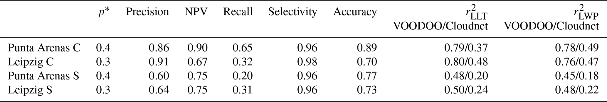
In this section, the predictive performance of the presented retrieval is investigated. First, in Sects. 4.1 and A, detailed analyses of two case studies from Punta Arenas and Leipzig are presented. Secondly, statistics for the entire 18-month-long data set are presented in Sect. 4.2. Table 4 shows an overview of achieved performance scores and correlation coefficients for both case studies and statistics.
Table 4Binary classification performance metrics and correlation coefficients with respect to MWR–LWP and adiabatic LWP from cloud liquid mask. Two case studies and the statistics from Punta Arenas and Leipzig are shown. The abbreviations C and S refer to case studies and statistics for the full data set, respectively.
4.1 Case study Punta Arenas
Figure 4 shows the observations from 1 August 2019 in Punta Arenas from a radar and lidar perspective. From 01:30 to 04:00 UTC, a mid-level stratiform cloud is present, which begins to form light precipitation about 30 min after observation onset. High βatt (Fig. 4d) indicates a liquid cloud top at about −15 ∘C in 3 km altitude, producing low amounts of small precipitating ice particles indicated by low m−1 sr−1 below the liquid layer. After 05:00 UTC, a multi-layer mixed-phase cloud was observed, indicated by high βatt (Fig. 4d), with liquid cloud base heights (LCBHs) of 1.3 and 2.8 km. From 06:00 UTC, the upper LCBH dropped to 2 km and then started to rise again. At 07:15 UTC the liquid layer continued to increase in altitude from 2.0–2.6 km at 08:45 UTC. During this time the reflectivity values ranging between −27 and +10 dBZ between 2.0–2.4 km altitude indicate a population of larger ice particles. Several smaller liquid-dominated clouds were observed by the ceilometer around 04:45 UTC at 4.7 km with temperatures ∘C, and after 05:30 UTC at 1.2 km ( ∘C), and 08:30 UTC at 0.5 km height (T<0 ∘C), where only some data points exceed the minimum detection capabilities of the cloud radar.
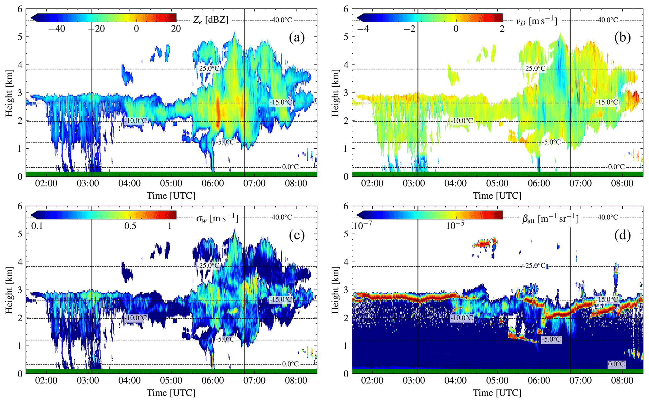
Figure 4Case study of 1 August 2019 in Punta Arenas, Chile. (a) Radar reflectivity factor Ze, (b) radar mean Doppler velocity , (c) radar spectrum width σw, and (d) ceilometer attenuated backscatter βatt. Dashed lines depict the isotherm lines from ECMWF temperature profiles. The green horizontal line at y axis = 0 indicates no rain was measured at ground. Solid vertical lines mark locations of the range spectrograms, shown in Fig. 7.
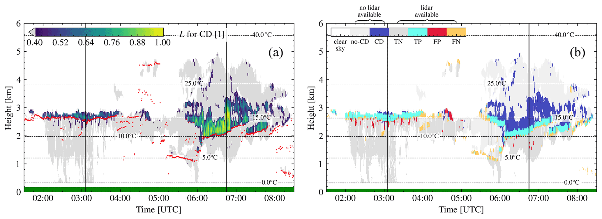
Figure 5Probability of the presence of cloud droplets for case study of 1 August 2019 in Punta Arenas, Chile. (a) VOODOO output: probability for CD. (b) VOODOO prediction status. Dashed lines depict the isotherm lines from ECMWF temperature profiles. Red dots in (a) indicate the first ceilometer CBH. The green horizontal line at y axis = 0 indicates no rain was measured at ground. Solid vertical lines mark locations of the range spectrograms, shown in Fig. 7.
Figure 5a shows the output of VOODOO with threshold (see Table 4), which provides a good compromise between FP and FN predictions. Light gray cells (L≤0.4) indicate noCD volumes and L>0.4 CD bearing, respectively. A visual comparison between bands of high βatt in Fig. 4d and predicted CD in Fig. 5a show good temporal and spatial agreement, as indicated by the cloud base plotted as red dots. Figure 5b shows a visual reference of CD false alarms marked by FP and CD misses marked by FN. With an accuracy = 0.890, almost 9 of 10 data points were correctly classified. An individual look at precision = 0.86 shows a false alarm rate (FAR = 1 − precision) of only 14 %, while a recall = 0.65 was achieved. Visible in Fig. 5b are TP (light blue) and TN (light gray), where the VOODOO predictions match the Cloudnet classification. In contrast, larger clusters of FN data points (yellow) occur mostly at liquid cloud base (02:00–04:00 UTC, at 2.7 km) and in thin pure liquid clouds (05:00–06:00 UTC at 1.3 km), thus reducing the recall value. Those FN predictions, which are responsible for the deviation of the recall from 1, are expected due to the lower sensitivity of the radar to liquid droplets compared to the lidar. Another cause of the FN predictions could be that liquid-only clouds or cloud volumes with low numbers of liquid droplets produce fewer Doppler spectra features, e.g., single peaks with low intensity or below noise floor or by superimposing the liquid peak on the much larger ice peak, which makes the features of the liquid peak disappear (i.e., non-separable from the ice). On the other hand, smaller clusters of FP predictions (red) occur below the ceilometer cloud base height (CBH). Those misclassifications are possibly caused by a higher spectrum width likely due to atmospheric turbulence. At the same time it should be noted that also Cloudnet's classification cannot be perfect even though it is used as ground truth here. This limits the achievable maximum of the quality metrics used in this study.
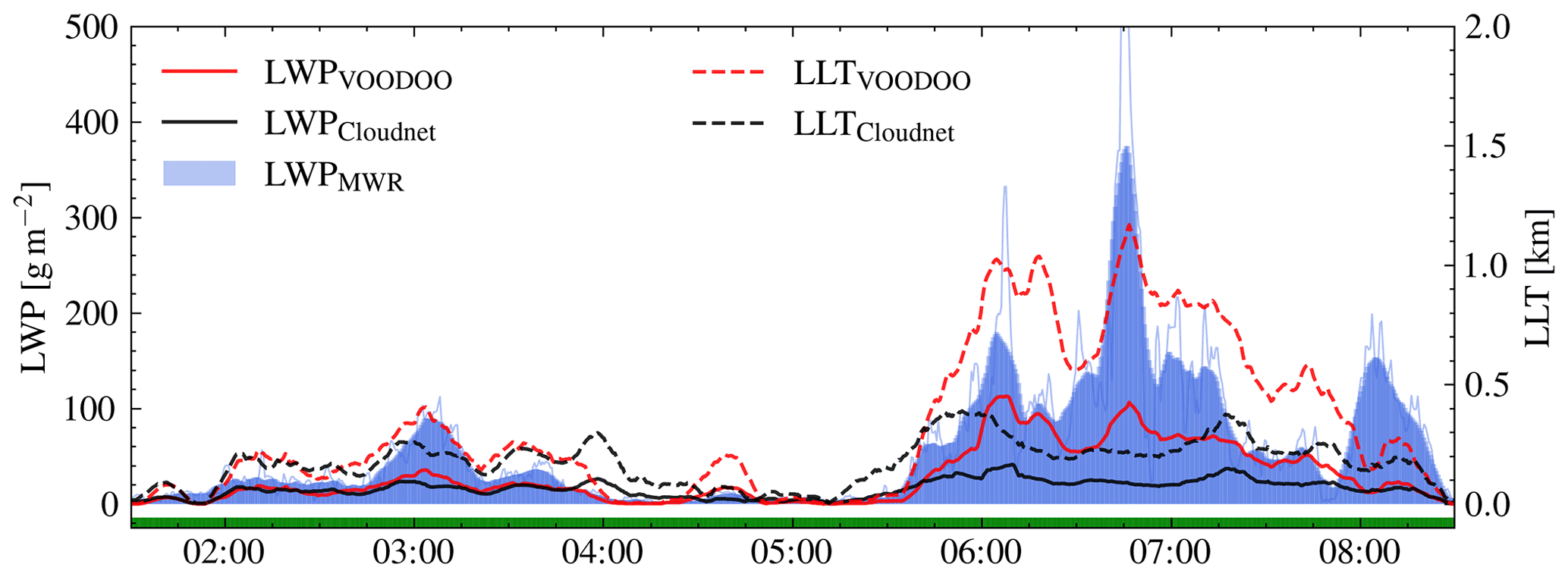
Figure 6Comparison of liquid water path (LWP) and liquid layer thickness (LLT) for the case study of 1 August 2019 in Punta Arenas, Chile. LWP (left y axis, solid lines) and LLT (right y axis, dashed lines). The thin blue line corresponds to original MWR–LWP time resolution and thick lines to 10 min smoothed data.
Note that there are approximately twice as many valid noCD than CD samples available in both data sets. This imbalance of the validation set makes the interpretation of performance metrics more difficult. Therefore, performance of VOODOO is validated on multiple binary classification metrics and independent observations from MWR. The LLT and LWPad (calculated according to Karstens et al., 1994) both correlate remarkably well with the measured MWR–LWP (see Fig. 6), reaching values for LLT (0.79) and LWP (0.78). In contrast, Cloudnet achieves significantly lower correlation coefficients with respect to LLT (0.37) and LWP (0.49). The geometric extent of liquid water layers retrieved with Cloudnet is only meaningful for optically thin and single-layer mixed-phase clouds, since the attenuated ceilometer signal (i.e., 06:00–08:00 UTC) cannot cover the complete liquid CD distribution in the atmosphere beyond lidar attenuation, thus underestimating the thickness of deep liquid-containing layers (see: black line in Fig. 6a).
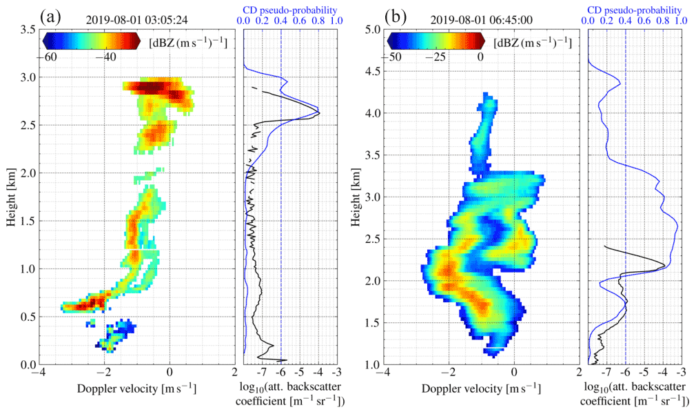
Figure 7Range spectrogram (left panel), attenuated backscatter coefficient (right panel, solid black line, bottom x ticks), and CD probability (right panel, solid blue line, top x ticks) profiles of 1 August 2019 in Punta Arenas, Chile. The dashed blue line highlights the decision threshold p∗ for the presence of cloud droplets. Panels (a) and (b) are samples for two different points in time (see black vertical lines in Figs. 4 and 5). The range spectrograms show bi-modal distributions (a) at 2.6–2.9 km and (b) at 2.1–2.9 km, coinciding in altitudes with the large peaks in the attenuated backscatter profile and matching the peaks in the predictions. The black line in the right subplot of (b) displays the attenuation of the ceilometer by total signal loss in the signal above 2.2 km altitude, while VOODOO is able to relate the bi-modal signature (left panel) to the presence of droplets above 2.2 km, as can be seen by the matching peak with the CD probability (blue line).
To illustrate the performance of VOODOO better, two range spectrograms, βatt, and CD pseudo-probability plots are shown in Fig. 7. In Fig. 7a, a bi-modal distribution is observed at altitudes between 2.6–2.9 km along with high ceilometer m−1 sr−1, indicating a population of liquid droplets near cloud top and matching the prediction of VOODOO with Cloudnet. Below 2.6 km, smaller ice crystals are falling out of the mixed-phase cloud top, which are melting and form drizzle drops at approximately 1 km altitude. Figure 7b shows the range spectrogram at 06:45:00 UTC. Cloud top is detected at 4.3 km, showing a mono-modal distribution at Doppler velocities of −1.5 to −0.5 m s−1. At 3.3 km altitude, the spectrum width suddenly increases rapidly, showing a skewed distribution with between −1.0 and 0.0 m s−1. As the altitude decreases, the spectrum splits into a clearly separable bi-modal distribution at altitudes below 3.0 km, indicating a CD population at 0 m s−1 Doppler velocity. The ceilometer shows a peak with high m−1 sr−1 at 2.2 km, matching the location of the bi-modality in the Doppler spectrum at the liquid layer base. Beyond an altitude of 2.4 km, the ceilometer is getting completely attenuated, such that Cloudnet's liquid droplet retrieval is not reliable anymore. In contrast, VOODOO is able to predict the entire range of the liquid layer from base (2.1 km) to top (3.1 km). Below, only one peak with increasing is visible in the spectrogram, which indicates that the larger ice crystals at higher Doppler velocities evaporate while precipitating out of the mixed-phase layer. A second case based on observations in Leipzig, Germany, is presented in Appendix A.
4.2 Statistical analysis of the performance of VOODOO
The statistical analysis is carried out by applying VOODOO to 18 months of observations from the two different geographical sites, excluding −10 % training data from Punta Arenas. This section discusses the ability of VOODOO to infer the presence of CD from Doppler radar spectrum features for a large data set spanning 1.5 years, which has not been done in previous studies. The Punta Arenas data set (PA) contains 220 d of observations (23 million data points), while the data from Leipzig (LE) count 342 d (30 million data points). Figure 8 shows the total numbers of validatable (lidar available) and non-validatable (no lidar available) data points. The numbers of negative samples TN + FP and noCD (i.e., ice, drizzle, or rain) are by far the most represented classes. The ratio of TN + FP to TP + FN (i.e., the ratio of validatable ice to liquid samples) is approximately 5 : 1 (PA) and 3 : 1 (LE), whereas the ratio of noCD to CD (i.e., the ratio of non-validatable ice and liquid samples) is 22 : 1 (PA) and 9 : 1 (LE). Our new approach predicts additional +50 % CD for PA and +100 % for LE beyond the lidar attenuation height. Note that the distribution is very sensitive to the p∗ threshold introduced in Sect. 3.3.
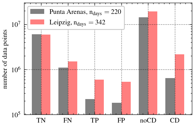
Figure 8Distribution of predicted lidar-validatable (TN, FN, TP, FP) and non-lidar-validatable (noCD, CD) data points.
Thresholds of p∗ for PA and LE are listed in Table 4. Two individual values for p∗ were chosen, to keep the false positive rate (FPR selectivity) below 5 % and maximize the number of correct predictions (TP and TN) while minimizing false predictions (FP and FN). The last two lines of Table 4 summarize the results found for the statistical evaluation, calculated with the sum of all valid classification results. The r2 columns represent the mean correlation coefficient over the entire data set.
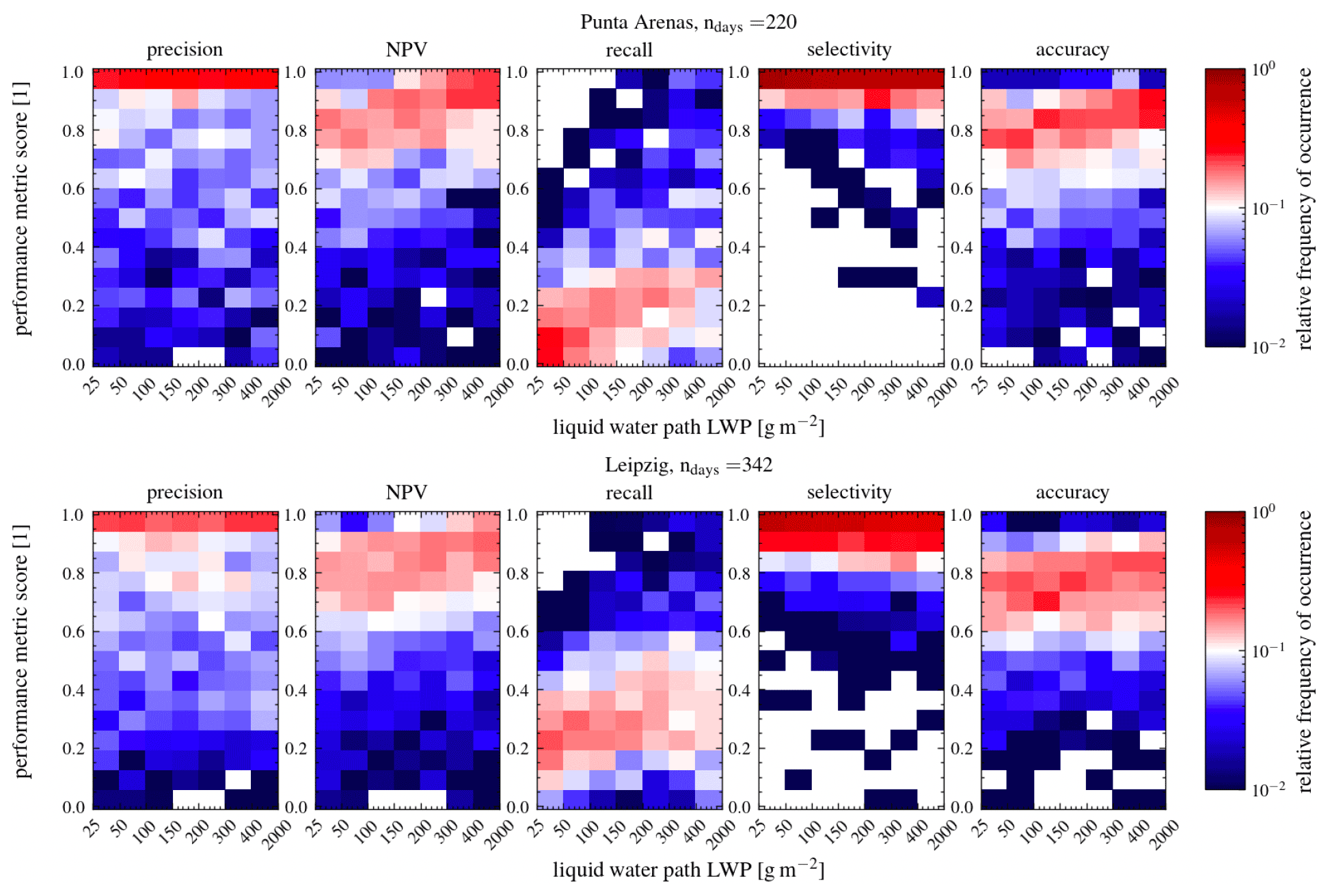
Figure 9Histograms of frequency of occurrence for each performance score as a function of LWP. The upper row shows Punta Arenas from 27 November 2018–29 September 2019, and the lower row shows Leipzig from 16 December 2020–6 March 2022. For all scores, a value of 1 represents the perfect score.
First, the performance is analyzed by means of relative frequencies of occurrence for a specific score (i.e., precision, recall) as a function of MWR–LWP. This gives an impression of how well VOODOO is able to reproduce the classification results provided by Cloudnet. The first column of Fig. 9 shows that the precision values have a clustering close to 1 over the whole LWP range. Nevertheless, the mean precision is 0.60 (PA) and 0.64 (LE). From this it follows that VOODOO is able to accurately relate cloud radar Doppler spectra features to CD presence, independently of LWP. The third columns of Fig. 9 show that the majority of occurrences of the recall are below values of 0.3. With increasing LWP, the recall score improves but generally stays quite low. More in-depth analysis of the prediction data reveals that the majority of missed CD samples (FN), which reduce the recall score, are found close to correctly identified CD samples (TP). Low recall is obtained for the uncertainty range of the MWR–LWP (LWP < 25 g m−2), where clouds contain almost no liquid water and the noCD samples predominate 10 to 1 over CD samples. The best scores are achieved for LWP > 100 g m−2. A visual reference is given by the two case studies in Figs. 5 and A2. These FNs are caused by the lower sensitivity of the radar to smaller populations of liquid cloud droplets or smaller sizes of cloud droplets compared to the ceilometer. In particular thin (supercooled) liquid-only clouds observed frequently over PA cause lower recall scores for this site. However, the linear increase in recall score with larger LWP values is more prominent in LE compared to PA, mostly due to the lower p∗ threshold. The accuracy values are 0.73 (LE) and 0.77 (PA). The accuracy scores (Fig. 9 column five) show most values are above 0.75, meaning three out of four samples were correctly classified, independent of LWP. Note that the LWP range below 50 g m−2 contains the largest absolute number of occurrences in the histogram.
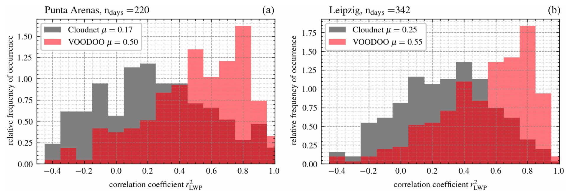
Figure 10Relative frequency of occurrence for correlation coefficients of MWR–LWP and LWPad. (a) Punta Arenas from 27 November 2018–29 September 2019 and (b) Leipzig from 16 December 2020–6 March 2022. Median μ of given in the legend.
The second statistical evaluation is carried out by analyzing the correlation coefficient between retrieved MWR–LWP and LWPad for each day of observation. Figure 10 shows the relative frequency of occurrence as a function of values. Both sites display similar distributions, with the CNN-based LWPad having stronger correlations with the MWR–LWP than Cloudnet-based LWPad. Median values μ for Cloudnet are 0.17 (PA) and 0.25 (LE), whereas VOODOO is able to improve the correlation of the LWP to 0.50 (PA) and 0.55 (LE). Despite the limits of this validation method, this shows that VOODOO is able to approximate the values of the MWR–LWP better compared to Cloudnet because it detects cloud droplets beyond the lidar attenuation. Thus, VOODOO's improved liquid detection (amount and location) can potentially improve higher-level retrieval products such as liquid water content. Note that the method of Karstens et al. (1994) uses the adiabatic assumption to calculate the liquid water path in combination with the liquid water mask (time–height mask for droplets presence) and ECMWF weather model data (temperature, air pressure, and specific humidity). Since the adiabatic assumption is not suitable in all cloud situations and the model data are subject to uncertainties, the idea was to compare only the correlation of both time series (MWR-LWP vs. LWPad of Cloudnet vs. LWPad of VOODOO). Therefore, we decided not to compare absolute values.
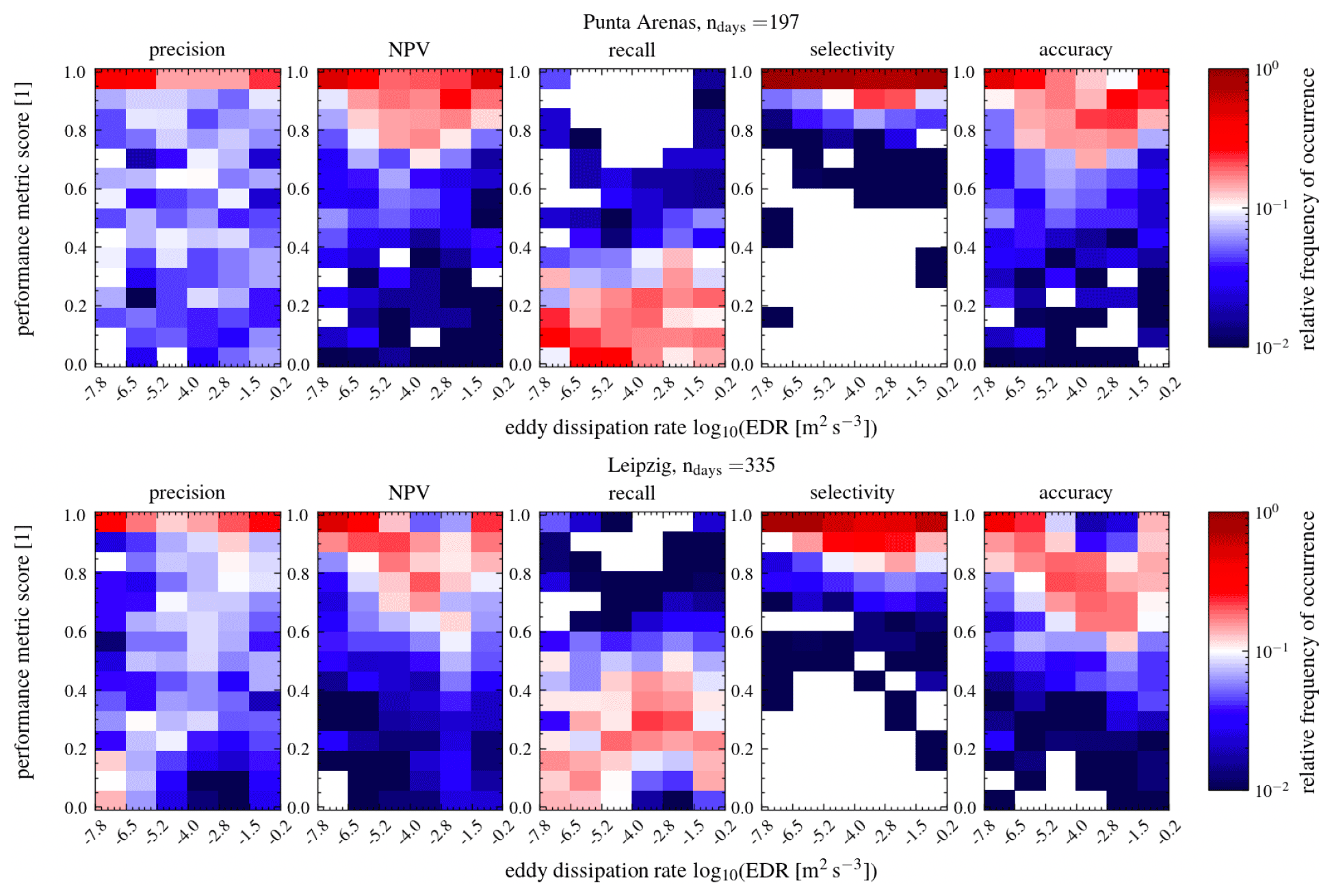
Figure 11Histograms of frequency of occurrence for each performance score as a function of εDR. The upper row shows Punta Arenas from 27 November 2018–29 September 2019, and the lower row shows Leipzig from 16 December 2020–6 March 2022. For all scores, a value of 1 represents the perfect score.
To evaluate the impact of turbulence on the VOODOO predictions, the relative frequency of performance scores as a function of turbulence eddy dissipation rate εDR within a range of in units of log 10 ([m2 s−3]) is displayed in Fig. 11. Note that the majority of data points (> 95 %) range between values of . The precision for PA and LE both shows most occurrences near a score of 1. However, the frequency of NPV scores near 1 decreases slightly as εDR increases, which can be caused by reducing the number of TNs or the increase in FN samples. Since recall performance improves slightly as the εDR increases, it follows that the number of FNs is reduced; thus most sample volumes containing no cloud droplets show low εDR. The accuracy score is mostly influenced by TN values; thus it follows the trend of the NPV. The selectivity scores, for both PA and LE, show a very narrow distribution near the perfect score 1. We can conclude that the influence of turbulence on the predictive performance of VOODOO is minor.
The supervised machine learning retrieval VOODOO is presented, which predicts the presence of cloud droplets from cloud radar Doppler spectra. Time spectrograms are processed by VOODOO, to directly predict a probability of the presence or absence of cloud droplets. The model is trained on long-term ground-based remote sensing observations from Punta Arenas in Chile. The a priori ground truth is given by the Cloudnet algorithm, which is a multi-instrument retrieval that processes radar, ceilometer, MWR, and ECMWF forecast model data into higher-level products (e.g., the atmospheric target classification). The performance is validated in detail on two case studies from different geographical locations, i.e., Punta Arenas, Chile, and Leipzig, Germany, located in the mid-latitudes of the Southern Hemisphere and Northern Hemisphere, respectively. This is done to test whether the trained CNN is also applicable for very different orographic conditions and aerosol loads influencing the occurrence of liquid-containing clouds and their properties over both sites. In addition to the case studies, for the first time, long-term observations of both sites are used to investigate the retrieval's robustness to new data.
The case study shows the ability of VOODOO to extract features from radar Doppler spectra and infer the presence of CD for the desired type of mixed-phase clouds. Due to the limitation of pixel-by-pixel comparison, instrument, and retrieval uncertainties, the design of the study does not allow a perfect score of 1. Nevertheless, for the long-term observations, VOODOO achieves good precision (>0.60) and accuracy (>0.73), confirmed indirectly by a strong correlation between MWR–LWP and LWPad (>0.45) compared to the correlation with LWPad of Cloudnet (<0.22). Due to lower sensitivity of cloud radar to small liquid droplets compared to lidar, the recall score is only <0.2. Overall, more FN predictions than FP predictions are responsible for this, with FNs occurring more frequently at the lowest range gates of liquid or mixed layers, or in thin and pure liquid layers (warm or supercooled) with low LWP. Overall, VOODOO performs best for (multi-layer) stratiform, deep mixed-phase cloud situations with LWP > 100 g m−2, where the number of liquid layers and the liquid layer depth often extend far more than previously assumed.
In conclusion, VOODOO performs best for (multi-layer) stratiform, deep mixed-phase cloud situations with LWP > 100 g m−2. From this analysis we learn that both Cloudnet and VOODOO have their strengths and weaknesses. Clearly, Cloudnet's lidar-based approach has an advantage in detecting thin liquid water layers, whereas VOODOO's radar approach can be used primarily to reveal hidden liquid water layers beyond lidar attenuation. Radar observations during strong precipitation (Cloudnet rain flag active), where no meaningful LWP can be retrieved from MWR observations, suffer strongly from liquid attenuation, and thus features in cloud radar Doppler spectra are less reliable (not shown). The thin (supercooled) liquid-only clouds show less pronounced spectral features and thus are more similar to single ice crystal peaks in the Doppler spectra and are, as a result, often misclassified.
It has been demonstrated that the VOODOO method could be a powerful addition to the existing Cloudnet target classification, making the detection of liquid layers beyond complete lidar attenuation possible. Additional validation methods are needed to better quantify the performance. These methods could include the comparisons of space-borne remote sensing observations with predictions to add cloud-top liquid-containing data points to the validation data set or air-borne in situ measurements for hydrometeor target classifications and radiation measurements with radiative closure studies (Barrientos Velasco et al., 2020). Note that all three mentioned ideas introduce their own uncertainties.
The ability to detect liquid beyond lidar attenuation is a major step in the field of Doppler spectrum-based analysis of vertically pointing ground-based radar observations. The described spectrum-based hydrometeor phase partition methodology can be regarded as a modular component applicable to Doppler cloud radar spectra. A synergy of the novel VOODOO and Cloudnet approaches would complement each other perfectly and is planned to be incorporated into the Cloudnet algorithm in the near future.
Note that the outlined technique has been tailored to an RPG-FMCW-94-DP cloud radar; other radars, ground-based or even space-borne (if Doppler spectra are available), may alter the quality of predictions. Therefore caution is advised in the generalization of the procedure to other Doppler radar systems. Still, the same architecture can simply be retrained on the radar Doppler spectra from another cloud radar, if a sufficiently large training data set is available.
To test whether VOODOO can be transferred to another location without re-training as suggested in Kalesse-Los et al. (2022), another example case is illustrated. Figure A1 shows observations for the second case study, which evaluates capabilities on validation data from Leipzig, Germany. Between 14:00 and 19:00 UTC on 30 December 2020, a multi-layer stratiform cloud situation was observed with cloud top at 1.2–1.5 km ( ∘C) for the first layer and 2.5–2.7 km ( ∘C) for the second cloud layer. Both layers with cloud-top temperatures below 0 ∘C contain supercooled liquid water, clearly visible between 1.0–1.5 km altitude (high values of βatt; see Fig. A1d).
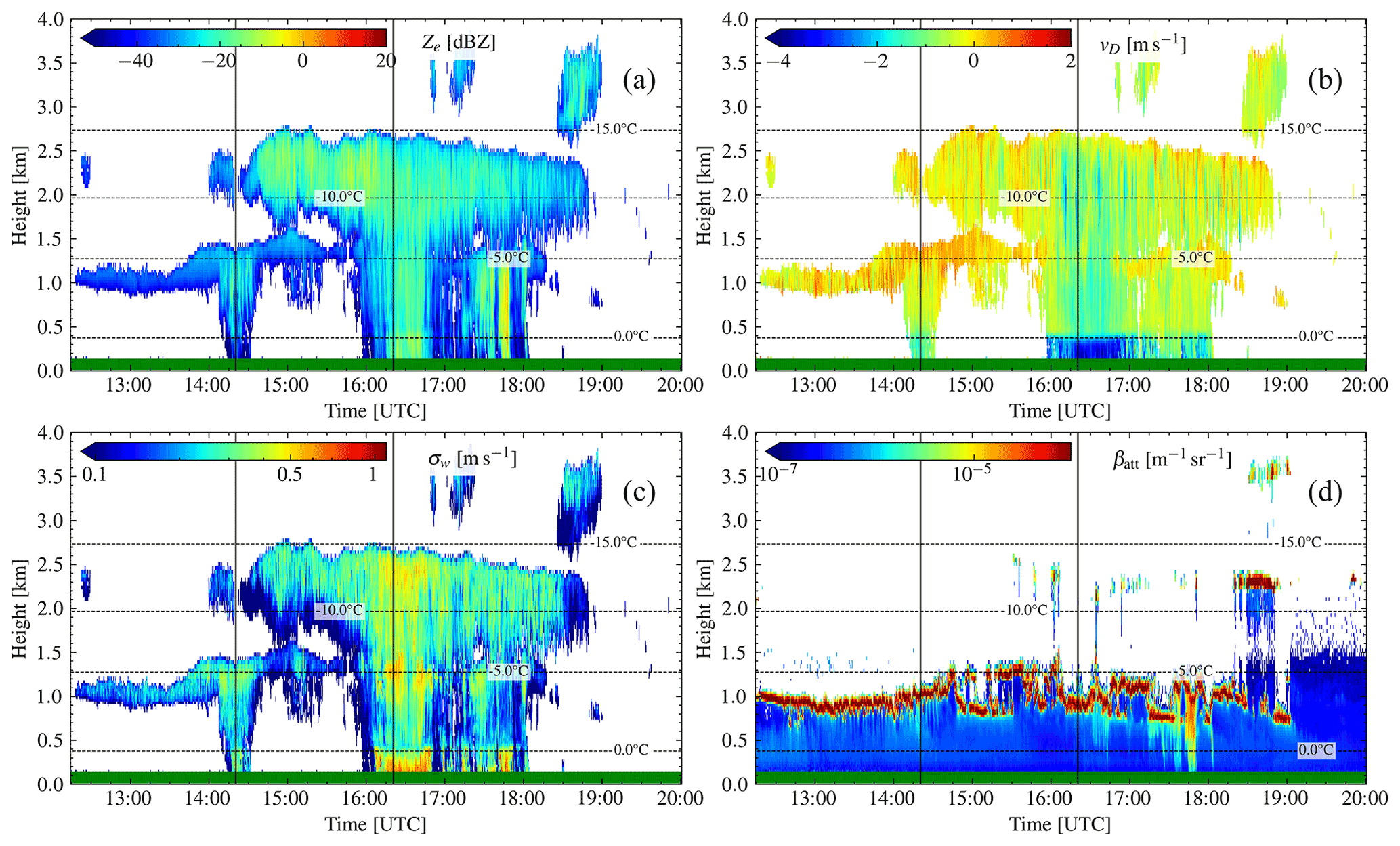
Figure A1Case study of 30 December 2020 in Leipzig, Germany. (a) Radar reflectivity factor Ze, (b) radar mean Doppler velocity , (c) radar spectrum width σw, and (d) ceilometer attenuated backscatter βatt. Dashed lines depict the isotherm lines from ECMWF temperature profiles. The green horizontal line at y axis = 0 indicates no rain was measured at ground. Solid vertical lines mark locations of the range spectrograms, shown in Fig. A4.
Based on the ceilometer observations, the first cloud base of a shallow low-level supercooled liquid cloud (12:30–14:00 UTC at 1.2 km) is at 1 km (indicated by red dots in Fig. A2a), which is 200 m below the predicted LCBH. The base of the low-level supercooled liquid cloud increases after 14:00 UTC when a second mixed-phase cloud (14:00–19:00 UTC) is observed with predicted liquid cloud top at 2.5 km. Further, smaller clouds at altitudes between 3.0–3.5 km and cloud-top temperatures of −20 ∘C are predicted to be cloud droplet bearing. These higher liquid-containing layers that are predicted by VOODOO are sporadically observed by the ceilometer, when it is able to penetrate the lower liquid layer at about 2.2–2.4 km and 3.5 km altitude. This refers to the TP data points in Fig. A2b.
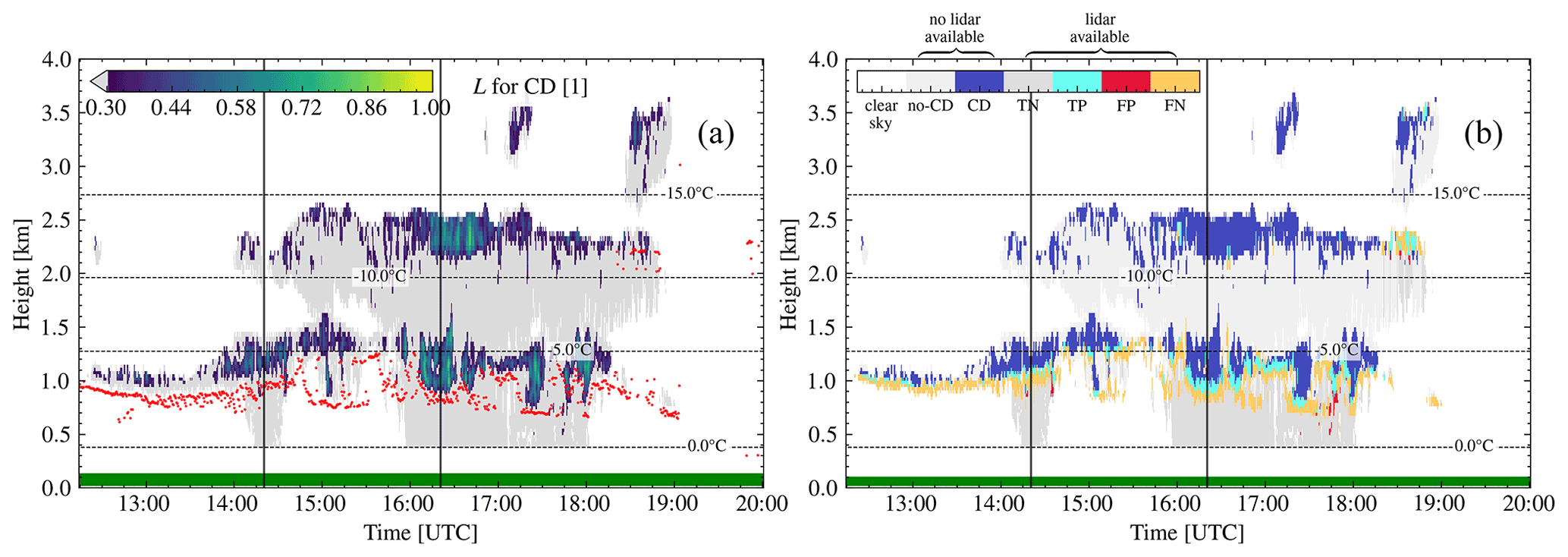
Figure A2Probability of the presence of cloud droplets for the case study of 30 December 2020 in Leipzig, Germany. (a) VOODOO output: probability of cloud droplets present. (b) VOODOO prediction status. Dashed lines depict the isotherm lines from ECMWF temperature profiles. Red dots in (a) indicate the first ceilometer CBH. The green horizontal line at y axis = 0 indicates no rain was measured at ground. Solid vertical lines mark locations of the range spectrograms, shown in Fig. A4.
For this case study, only very few FPs at 17:45 UTC (at 0.75 km) and 18:30 UTC (at 2.2 km) were predicted (see Fig. A2b), resulting in a high precision for this case of 0.91. Predicted FN data points, approximately at CBH detected by the ceilometer (see Fig. A2b, yellow pixel), result in a recall score of 0.32. This effect is caused by cloud edge filtering and lower radar sensitivity to liquid cloud droplets (i.e., the ceilometer being able to detect smaller numbers of CD and smaller CD). VOODOO achieves a high accuracy of 0.70. Further, VOODOO displays a much better agreement with temporal evolution of LLT and LWP compared to MWR–LWP (see Fig. A3), achieving larger and of 0.80 and 0.76 compared to the values for Cloudnet (0.48 and 0.47; see Table 4).
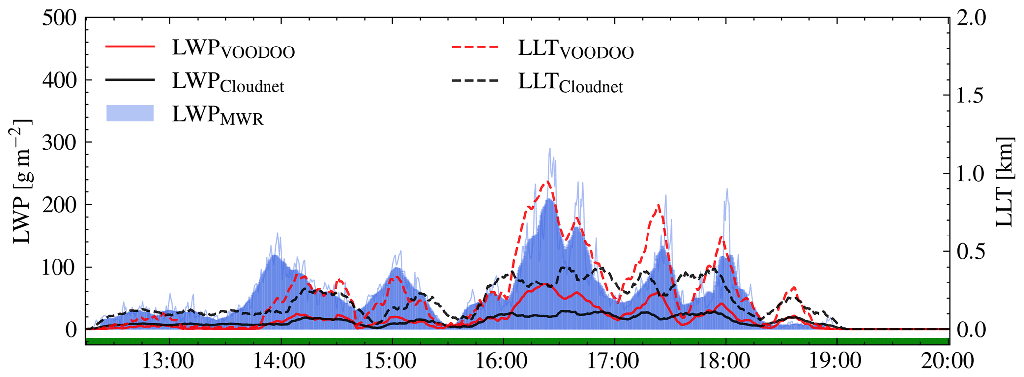
Figure A3Comparison of liquid water path (LWP) and liquid layer thickness (LLT) for the case study of 30 December 2020 in Leipzig, Germany. LWP (left y axis, solid lines) and LLT (right y axis, dashed lines). The thin blue line corresponds to original MWR–LWP time resolution and thick lines to 10 min smoothed data.
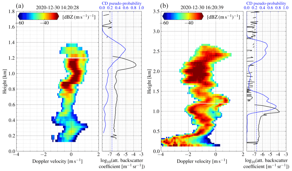
Figure A4Range spectrogram (left panel), attenuated backscatter coefficient (right panel, solid black line, bottom x ticks), and CD probability (right panel, solid blue line, top x ticks) profiles of 30 December 2020 in Leipzig, Germany. The dashed blue line highlights the decision threshold p∗ for the presence of cloud droplets. Panels (a) and (b) are samples for two different points in time (see black vertical lines in Figs. A1 and A2). The left panel shows bi-modal distributions (a) at 1.1–1.3 km and (b) at 0.8– 1.4 km, coinciding in altitudes with the large peaks in the attenuated backscatter profile and matching the peaks in the predictions. More liquid is found by VOODOO in (b) at cloud top (2.3–2.7 km) with enhanced spectrum width and centered near 0 m s−1.
Figure A4 displays the range spectrogram, attenuated backscatter coefficient, and probability profiles for two time steps, indicated by vertical black lines in Figs. A1 and A2. The liquid contribution to the bi-modal radar returns is clearly visible in Fig. A4a at cloud top between 1.1–1.4 km. Below 1.1 km, the bi-modal peak merges into one peak, resulting in a mono-modal distribution. In the transition above 1.1 km VOODOO could infer the presence cloud droplets, while the more sensitive ceilometer could detect the liquid cloud base one range gate below. In contrast, below liquid cloud base all noCD predictions were classified correctly by VOODOO. After 14:00 UTC a multi-layer cloud situation is observed and investigated through the second range spectrogram (Fig. A4b). At cloud top (2.5 km altitude and ∘C) the spectrum shows a skewed distribution with high σw and at approximately 0 m s−1. VOODOO predicts the probability for CD > 0.3. At 1.0–1.5 km ( ∘C) another liquid bearing layer is revealed by VOODOO, indicated by the bi-modal distribution, where the liquid contribution shifts from 0 to 1 m s−1 within a 500 m range, indicating an updraft at liquid layer top. In both profiles, VOODOO demonstrated the capability to infer the presence of CD also for regions with higher spectrum width, even without clearly separated spectral features (i.e., bi-modalities).
A detailed discussion of the PDFs of different variables is listed below, given the notation , with and used to distinguish individual distributions for the two Figs. B1 and B2.

Figure B1Probability density functions (PDFs) for different variables obtained in Punta Arenas, Chile.
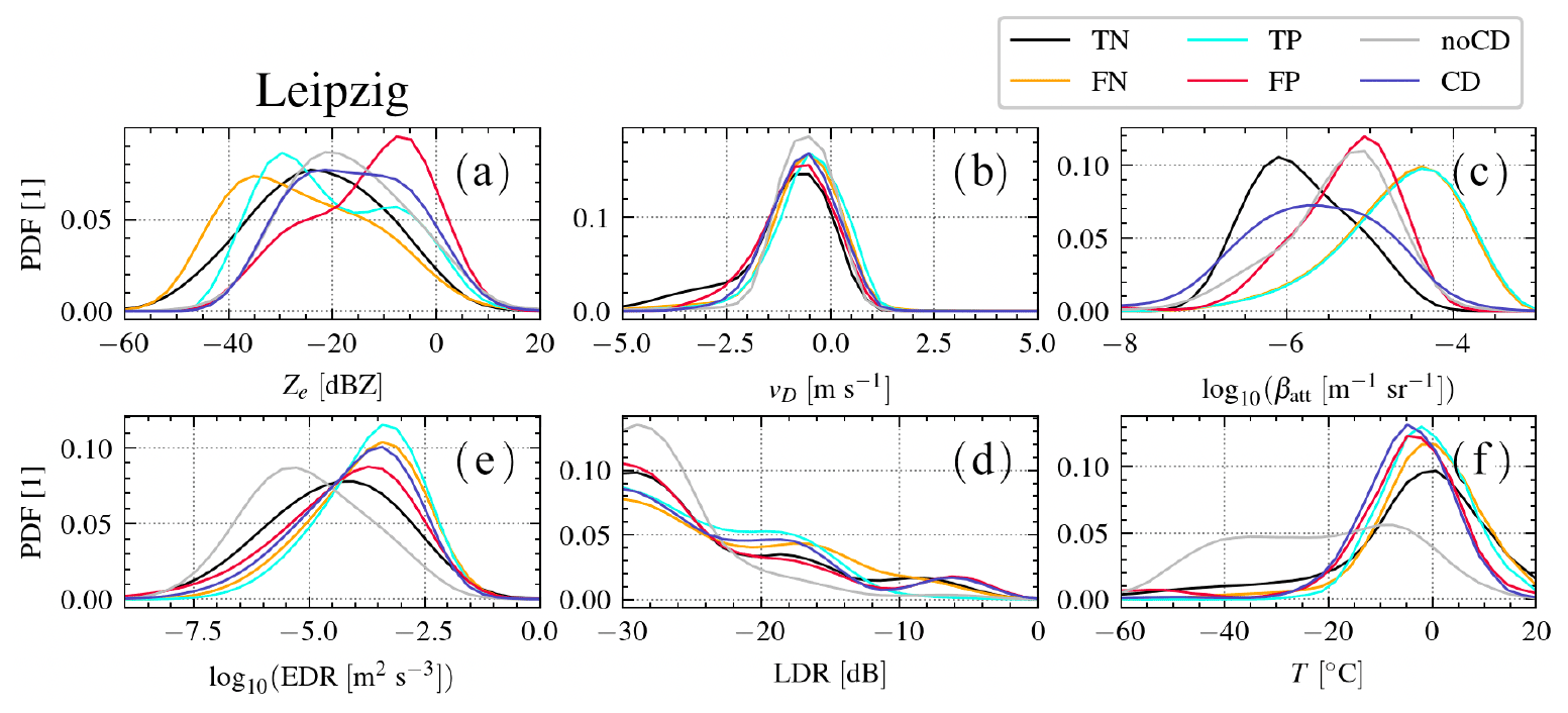
Figure B2Probability density functions (PDFs) for different variables obtained in Leipzig, Germany.
- a.
Radar reflectivity factor Ze in units of dBZ.
shows two distinct peaks at −30 dBZ for both PA and LE (i.e., liquid-only clouds) and a second peak at −10 dBZ for PA and −7 dBZ for LE (i.e., mixed-phase clouds). shows a single peak centered at approx. −23 dBZ for both PA and LE with large variance. for the PA data shows two separable peaks centered at −28 dBZ (lower amplitude) and −2 dBZ (larger amplitude). However, the two peaks in for LE data are at −26 dBZ (liquid-dominated mixed-phase clouds) and −7 dBZ (ice-dominated mixed-phase volumes). shows a slightly skewed distribution for both PA and LE with peaks at −36 dBZ (LE) and −27 dBZ (PA), indicating that most volumes with cloud droplets which were not correctly predicted by VOODOO have low reflectivity. Nevertheless, the LE data have a much more positively skewed (mode < median < mean) distribution, containing a potential second peak within dBZ. for PA shows two peaks at −22 and −5 dBZ, where the latter one is likely associated with ice or drizzle that is misclassified as CD. show positive skewed distributions for both sites, centered at −18 dBZ for PA and −20 dBZ for LE. - b.
Radar mean Doppler velocity in units of m s−1.
shows similar morphologies (e.g., center values in , mono-modal) for all classes and both sites. Due to the orographically induced gravity waves at PA, the distributions show larger variance, where the peak in is located closer to 0 m s−1. - c.
log 10 of lidar attenuated backscatter coefficient βatt in units of log 10 (m−1 sr−1). and distributions match very well for both LE and PA, showing negative skewness with peaks between −4.7 and −4.4, respectively. Most values correspond to low βatt values (expected for ice crystals), were PA data show a peak at −7, which is noticeably lower than the peak for LE data at −5.2. values show distributions with peaks between , where potentially larger numbers of small ice crystals were observed. Note that and refer to lidar observations beyond thin liquid layers. Those data points are influenced by attenuation effects from liquid layers in lower altitudes and thus were excluded from analysis.
- d.
log 10 of eddy dissipation rate εDR in units of m2 s−3.
is centered at −3.5 and at −4.5 for both PA and LE. However, the peak in the noCD distribution shows the maxima at approx. −5.5. Assuming that liquid bearing layers are usually more turbulent than precipitating ice crystals (Luke et al., 2010), a peak at lower values in predictions is expected. shows its peak at large values of −3.8, matching the peak of . and present a good fit. Overall, LE shows higher turbulence values than PA. - e.
Radar linear depolarization ratio (LDR) in units of dB. The LDR distribution for PA fLDR shows two distinct peaks at −30 (spherical particles) and −20 (columns) and three peaks at −30 (spherical), −20 to −15 (columns), and −5 (insects embedded in clouds) for LE.
- f.
model temperature T in units of ∘C.
The distributions of values in C (Eq. 7) and CD show single peaks centered between −10 and 0. spreads over a larger T range of that is indicative of regions where ice particles (noCD) are detected for T<0 and drizzle or rain at T>0.
The ground-based remote sensing data used in this article are generated by the European Research Infrastructure for the observation of Aerosol, Clouds and Trace Gases (ACTRIS) and are available from the ACTRIS Data Centre using the following link: https://hdl.handle.net/21.12132/2.d2bcddcd9355409e (last access: 12 September 2022, CLU, 2022). The machine learning results will be incorporated into the Cloudnet data processing chain and will also be available via ACTRIS in the future. Meanwhile, they can be reprocessed via VOODOO (https://doi.org/10.5281/zenodo.5970206, Schimmel, 2022) or obtained upon request from willi.schimmel@uni-leipzig.de. A setup of pyLARDA (https://doi.org/10.5281/zenodo.4721311, Bühl et al., 2021) was used for data input and analysis. Cloudnet processing was done using CloudnetPy (https://doi.org/10.5281/zenodo.4011843, Tukiainen et al., 2020b, a).
The method was developed by WS with contributions by HKL and TV. PS provided the DACAPO-PESO ceilometer and MWR data. WS performed data visualization and analysis with help from TV, HKL, MM, PSG, AF, and PS. The text was written by WS and reviewed by all co-authors.
At least one of the (co-)authors is a member of the editorial board of Atmospheric Measurement Techniques. The peer-review process was guided by an independent editor, and the authors also have no other competing interests to declare.
Publisher’s note: Copernicus Publications remains neutral with regard to jurisdictional claims in published maps and institutional affiliations.
The measurements from Punta Arenas were produced by the Leibniz Institute for Tropospheric Research using resources provided by the Finnish Meteorological Institute and acquired in the framework of the field experiment Dynamics, Aerosol, Clouds and Precipitation Observations in the Pristine Environment of the Southern Ocean (DACAPO-PESO), a research initiative from the Leibniz Institute for Tropospheric Research, Leipzig, Germany, in joint collaboration with the University of Magallanes, Punta Arenas, Chile, and the University of Leipzig, Leipzig, Germany. We acknowledge the provision of physical access to the LACROS resources in the framework of DACAPO-PESO and the European Research Infrastructure for the observation of Aerosol, Clouds and Trace Gases (ACTRIS) as part of the European Union's Horizon 2020 research and innovation program. We also acknowledge ECMWF for providing Integrated Forecasting System (IFS) model data. Further, we want to thank Boris Barja from the Universidad de Magallanes for granting access to the site and his support throughout the field campaign. Special thanks to Simo Tukiainen (FMI) for Cloudnet support and Teresa Vogl and Martin Radenz (TROPOS) for their remote sensing and programming expertise. We also thank Marika Kaden (Mittweida University of Applied Sciences) for the advice on machine learning.
This research has been supported by the Federal State of Saxony and the European Social Fund (ESF) in the framework of the program “Projects in the fields of higher education and research” (grant no. 100339509) and ESF-REACT (grant no. 100602743); it was supported by the Open Access Publishing Fund of Leipzig University. Parts of the DACAPO-PESO campaign were funded by the Deutsche Forschungsgemeinschaft (DFG – German Research Foundation) project PICNICC (grant nos. SE2464/1-1 and KA4162/2-1) accessible via ACTRIS (grant nos. 654109 and 739530).
This paper was edited by Jian Xu and reviewed by two anonymous referees.
Alexander, S. P., Sato, K., Watanabe, S., Kawatani, Y., and Murphy, D. J.: Southern Hemisphere Extratropical Gravity Wave Sources and Intermittency Revealed by a Middle-Atmosphere General Circulation Model, J. Atmos. Sci., 73, 1335–1349, https://doi.org/10.1175/JAS-D-15-0149.1, 2016. a
Alexander, S. P., Orr, A., Webster, S., and Murphy, D. J.: Observations and fine-scale model simulations of gravity waves over Davis, East Antarctica (69∘ S, 78∘ E), J. Geophys. Res.-Atmos., 122, 7355–7370, https://doi.org/10.1002/2017JD026615, 2017. a
Ansmann, A., Mattis, I., Müller, D., Wandinger, U., Radlach, M., Althausen, D., and Damoah, R.: Ice formation in Saharan dust over central Europe observed with temperature/humidity/aerosol Raman lidar, J. Geophys. Res.-Atmos., 110, D18S12, https://doi.org/10.1029/2004JD005000, 2005. a
Baars, H., Kanitz, T., Engelmann, R., Althausen, D., Heese, B., Komppula, M., Preißler, J., Tesche, M., Ansmann, A., Wandinger, U., Lim, J.-H., Ahn, J. Y., Stachlewska, I. S., Amiridis, V., Marinou, E., Seifert, P., Hofer, J., Skupin, A., Schneider, F., Bohlmann, S., Foth, A., Bley, S., Pfüller, A., Giannakaki, E., Lihavainen, H., Viisanen, Y., Hooda, R. K., Pereira, S. N., Bortoli, D., Wagner, F., Mattis, I., Janicka, L., Markowicz, K. M., Achtert, P., Artaxo, P., Pauliquevis, T., Souza, R. A. F., Sharma, V. P., van Zyl, P. G., Beukes, J. P., Sun, J., Rohwer, E. G., Deng, R., Mamouri, R.-E., and Zamorano, F.: An overview of the first decade of PollyNET: an emerging network of automated Raman-polarization lidars for continuous aerosol profiling, Atmos. Chem. Phys., 16, 5111–5137, https://doi.org/10.5194/acp-16-5111-2016, 2016. a
Barrientos Velasco, C., Deneke, H., Griesche, H., Seifert, P., Engelmann, R., and Macke, A.: Spatiotemporal variability of solar radiation introduced by clouds over Arctic sea ice, Atmos. Meas. Tech., 13, 1757–1775, https://doi.org/10.5194/amt-13-1757-2020, 2020. a
Bjordal, J., Storelvmo, T., Alterskjær, K., and Carlsen, T.: Equilibrium climate sensitivity above 5 ∘C plausible due to state-dependent cloud feedback, Nat. Geosci., 13, 718–721, https://doi.org/10.1038/s41561-020-00649-1, 2020. a
Borque, P., Luke, E., and Kollias, P.: On the unified estimation of turbulence eddy dissipation rate using Doppler cloud radars and lidars, J. Geophys. Res.-Atmos., 121, 5972–5989, https://doi.org/10.1002/2015jd024543, 2016. a
Bromwich, D. H., Werner, K., Casati, B., Powers, J. G., Gorodetskaya, I. V., Massonnet, F., Vitale, V., Heinrich, V. J., Liggett, D., Arndt, S., Barja, B., Bazile, E., Carpentier, S., Carrasco, J. F., Choi, T., Choi, Y., Colwell, S. R., Cordero, R. R., Gervasi, M., Haiden, T., Hirasawa, N., Inoue, J., Jung, T., Kalesse, H., Kim, S.-J., Lazzara, M. A., Manning, K. W., Norris, K., Park, S.-J., Reid, P., Rigor, I., Rowe, P. M., Schmithüsen, H., Seifert, P., Sun, Q., Uttal, T., Zannoni, M., and Zou, X.: The Year of Polar Prediction in the Southern Hemisphere (YOPP-SH), B. Am. Meteorol. Soc., 101, E1653–E1676, https://doi.org/10.1175/bams-d-19-0255.1, 2020. a
Bühl, J., Ansmann, A., Seifert, P., Baars, H., and Engelmann, R.: Toward a quantitative characterization of heterogeneous ice formation with lidar/radar: Comparison of CALIPSO/CloudSat with ground-based observations, Geophys. Res. Lett., 40, 4404–4408, https://doi.org/10.1002/grl.50792, 2013. a
Bühl, J., Seifert, P., Myagkov, A., and Ansmann, A.: Measuring ice- and liquid-water properties in mixed-phase cloud layers at the Leipzig Cloudnet station, Atmos. Chem. Phys., 16, 10609–10620, https://doi.org/10.5194/acp-16-10609-2016, 2016. a
Bühl, J., Radenz, M., Schimmel, W., Vogl, T., Röttenbacher, J., and Lochmann, M.: pyLARDA v3.2 (v3.2), Zenodo [code], https://doi.org/10.5281/zenodo.4721311, 2021. a
Choi, Y.-S., Ho, C.-H., Park, C.-E., Storelvmo, T., and Tan, I.: Influence of cloud phase composition on climate feedbacks, J. Geophys. Res.-Atmos., 119, 3687–3700, https://doi.org/10.1002/2013JD020582, 2014. a
CLU: Cloud profiling products: Classification, Categorize; cloud profiling measurements: Lidar, Microwave radiometer, Radar; ecmwf model data; 2018-11-27 to 2019-09-28; from Punta-Arenas, generated by the cloud profiling unit of the ACTRIS Data Centre [data set], https://hdl.handle.net/21.12132/2.d2bcddcd9355409e, last access: 12 Septemer 2022. a
de Boer, G., Eloranta, E. W., and Shupe, M. D.: Arctic Mixed-Phase Stratiform Cloud Properties from Multiple Years of Surface-Based Measurements at Two High-Latitude Locations, J. Atmos. Sci., 66, 2874–2887, https://doi.org/10.1175/2009JAS3029.1, 2009. a
Floutsi, A. A., Baars, H., Radenz, M., Haarig, M., Yin, Z., Seifert, P., Jimenez, C., Ansmann, A., Engelmann, R., Barja, B., Zamorano, F., and Wandinger, U.: Advection of Biomass Burning Aerosols towards the Southern Hemispheric Mid-Latitude Station of Punta Arenas as Observed with Multiwavelength Polarization Raman Lidar, Remote Sens., 13, 138, https://doi.org/10.3390/rs13010138, 2021. a, b
Foth, A. and Pospichal, B.: Optimal estimation of water vapour profiles using a combination of Raman lidar and microwave radiometer, Atmos. Meas. Tech., 10, 3325–3344, https://doi.org/10.5194/amt-10-3325-2017, 2017. a
Foth, A., Kanitz, T., Engelmann, R., Baars, H., Radenz, M., Seifert, P., Barja, B., Fromm, M., Kalesse, H., and Ansmann, A.: Vertical aerosol distribution in the southern hemispheric midlatitudes as observed with lidar in Punta Arenas, Chile (53.2∘ S and 70.9∘ W), during ALPACA, Atmos. Chem. Phys., 19, 6217–6233, https://doi.org/10.5194/acp-19-6217-2019, 2019. a
Goodfellow, I., Bengio, Y., and Courville, A.: Deep Learning, MIT Press, http://www.deeplearningbook.org (last access: 12 Septemer 2022), 2016. a, b
Goodfellow, I. J., Bulatov, Y., Ibarz, J., Arnoud, S., and Shet, V.: Multi-digit Number Recognition from Street View Imagery using Deep Convolutional Neural Networks, arXiv [preprint], https://doi.org/10.48550/ARXIV.1312.6082, 20 December 2013. a
Griesche, H. J., Seifert, P., Ansmann, A., Baars, H., Barrientos Velasco, C., Bühl, J., Engelmann, R., Radenz, M., Zhenping, Y., and Macke, A.: Application of the shipborne remote sensing supersite OCEANET for profiling of Arctic aerosols and clouds during Polarstern cruise PS106, Atmos. Meas. Tech., 13, 5335–5358, https://doi.org/10.5194/amt-13-5335-2020, 2020. a
Hecht-Nielsen, R.: Theory of the backpropagation neural network, in: International 1989 Joint Conference on Neural Networks, 18–22 June 1989, Washington, D.C., USA, vol. 1, 593–605, https://doi.org/10.1109/IJCNN.1989.118638, 1989. a, b
Heese, B., Flentje, H., Althausen, D., Ansmann, A., and Frey, S.: Ceilometer lidar comparison: backscatter coefficient retrieval and signal-to-noise ratio determination, Atmos. Meas. Tech., 3, 1763–1770, https://doi.org/10.5194/amt-3-1763-2010, 2010. a
Hildebrand, P. H. and Sekhon, R. S.: Objective Determination of the Noise Level in Doppler Spectra, J. Appl. Meteor., 13, 808–811, https://doi.org/10.1175/1520-0450(1974)013<0808:odotnl>2.0.co;2, 1974. a
Illingworth, A. J., Hogan, R. J., O'Connor, E., Bouniol, D., Brooks, M. E., Delanoé, J., Donovan, D. P., Eastment, J. D., Gaussiat, N., Goddard, J. W. F., Haeffelin, M., Baltink, H. K., Krasnov, O. A., Pelon, J., Piriou, J.-M., Protat, A., Russchenberg, H. W. J., Seifert, A., Tompkins, A. M., van Zadelhoff, G.-J., Vinit, F., Willén, U., Wilson, D. R., and Wrench, C. L.: Cloudnet: Continuous Evaluation of Cloud Profiles in Seven Operational Models Using Ground-Based Observations, B. Am. Meteorol. Soc., 88, 883–898, https://doi.org/10.1175/BAMS-88-6-883, 2007. a, b, c, d
Jimenez, C., Ansmann, A., Engelmann, R., Donovan, D., Malinka, A., Seifert, P., Wiesen, R., Radenz, M., Yin, Z., Bühl, J., Schmidt, J., Barja, B., and Wandinger, U.: The dual-field-of-view polarization lidar technique: a new concept in monitoring aerosol effects in liquid-water clouds – case studies, Atmos. Chem. Phys., 20, 15265–15284, https://doi.org/10.5194/acp-20-15265-2020, 2020. a, b
Kalesse, H., Vogl, T., Paduraru, C., and Luke, E.: Development and validation of a supervised machine learning radar Doppler spectra peak-finding algorithm, Atmos. Meas. Tech., 12, 4591–4617, https://doi.org/10.5194/amt-12-4591-2019, 2019. a, b, c
Kalesse-Los, H., Schimmel, W., Luke, E., and Seifert, P.: Evaluating cloud liquid detection against Cloudnet using cloud radar Doppler spectra in a pre-trained artificial neural network, Atmos. Meas. Tech., 15, 279–295, https://doi.org/10.5194/amt-15-279-2022, 2022. a, b, c, d, e, f
Kalogeras, P., Battaglia, A., and Kollias, P.: Supercooled Liquid Water Detection Capabilities from Ka-Band Doppler Profiling Radars: Moment-Based Algorithm Formulation and Assessment, Remote Sens., 13, 2891, https://doi.org/10.3390/rs13152891, 2021. a
Kanitz, T., Seifert, P., Ansmann, A., Engelmann, R., Althausen, D., Casiccia, C., and Rohwer, E. G.: Contrasting the impact of aerosols at northern and southern midlatitudes on heterogeneous ice formation, Geophys. Res. Lett., 38, L17802, https://doi.org/10.1029/2011GL048532, 2011. a
Karstens, U., Simmer, C., and Ruprecht, E.: Remote sensing of cloud liquid water, Meteorol. Atmos. Phys., 54, 157–171, https://doi.org/10.1007/BF01030057, 1994. a, b, c, d
Kelley, H. J.: Gradient theory of optimal flight paths, American Rocket Society Journal, 30, 947–954, 1960. a, b
Kingma, D. P. and Ba, J.: Adam: A Method for Stochastic Optimization, arXiv [preprint], https://doi.org/10.48550/arXiv.1412.6980, 30 January 2017. a
Kollias, P., Miller, M. A., Luke, E. P., Johnson, K. L., Clothiaux, E. E., Moran, K. P., Widener, K. B., and Albrecht, B. A.: The Atmospheric Radiation Measurement Program Cloud Profiling Radars: Second-Generation Sampling Strategies, Processing, and Cloud Data Products, J. Atmos. Ocean. Tech., 24, 1199–1214, https://doi.org/10.1175/jtech2033.1, 2007. a
Krizhevsky, A., Sutskever, I., and Hinton, G. E.: ImageNet Classification with Deep Convolutional Neural Networks, in: Advances in Neural Information Processing Systems, edited by: Pereira, F., Burges, C. J. C., Bottou, L., and Weinberger, K. Q., vol. 25, Curran Associates, Inc., https://proceedings.neurips.cc/paper/2012/file/c399862d3b9d6b76c8436e924a68c45b-Paper.pdf (last access: 12 September 2022), 2012. a
Küchler, N., Kneifel, S., Löhnert, U., Kollias, P., Czekala, H., and Rose, T.: A W-Band Radar–Radiometer System for Accurate and Continuous Monitoring of Clouds and Precipitation, J. Atmos. Ocean. Tech., 34, 2375–2392, https://doi.org/10.1175/jtech-d-17-0019.1, 2017. a
LeCun, Y., Boser, B., Denker, J. S., Henderson, D., Howard, R. E., Hubbard, W., and Jackel, L. D.: Backpropagation Applied to Handwritten Zip Code Recognition, Neural Comput., 1, 541–551, https://doi.org/10.1162/neco.1989.1.4.541, 1989. a, b
LeCun, Y., Bengio, Y., and Hinton, G.: Deep learning, Nature, 521, 436–444, https://doi.org/10.1038/nature14539, 2015. a
Luke, E. P., Kollias, P., Johnson, K. L., and Clothiaux, E. E.: A Technique for the Automatic Detection of Insect Clutter in Cloud Radar Returns, J. Atmos. Ocean. Tech., 25, 1498–1513, https://doi.org/10.1175/2007JTECHA953.1, 2008. a, b
Luke, E. P., Kollias, P., and Shupe, M. D.: Detection of supercooled liquid in mixed-phase clouds using radar Doppler spectra, J. Geophys. Res. Atmos., 115, D19201, https://doi.org/10.1029/2009JD012884, 2010. a, b, c, d, e, f, g, h, i
Maskey, M., Alemohammad, H., Murphy, K., and Ramachandran, R.: Advancing AI for Earth Science: A Data Systems Perspective, Eos, 101, https://doi.org/10.1029/2020eo151245, 2020. a
Morrison, H., de Boer, G., Feingold, G., Harrington, J., Shupe, M. D., and Sulia, K.: Resilience of persistent Arctic mixed-phase clouds, Nat. Geosci., 5, 11–17, https://doi.org/10.1038/ngeo1332, 2012. a
Mülmenstädt, J., Sourdeval, O., Delanoë, J., and Quaas, J.: Frequency of occurrence of rain from liquid-, mixed-, and ice-phase clouds derived from A-Train satellite retrievals, Geophys. Res. Lett., 42, 6502–6509, https://doi.org/10.1002/2015GL064604, 2015. a
Myagkov, A., Seifert, P., Bauer-Pfundstein, M., and Wandinger, U.: Cloud radar with hybrid mode towards estimation of shape and orientation of ice crystals, Atmos. Meas. Tech., 9, 469–489, https://doi.org/10.5194/amt-9-469-2016, 2016a. a
Myagkov, A., Seifert, P., Wandinger, U., Bühl, J., and Engelmann, R.: Relationship between temperature and apparent shape of pristine ice crystals derived from polarimetric cloud radar observations during the ACCEPT campaign, Atmos. Meas. Tech., 9, 3739–3754, https://doi.org/10.5194/amt-9-3739-2016, 2016b. a
Ohneiser, K., Ansmann, A., Baars, H., Seifert, P., Barja, B., Jimenez, C., Radenz, M., Teisseire, A., Floutsi, A., Haarig, M., Foth, A., Chudnovsky, A., Engelmann, R., Zamorano, F., Bühl, J., and Wandinger, U.: Smoke of extreme Australian bushfires observed in the stratosphere over Punta Arenas, Chile, in January 2020: optical thickness, lidar ratios, and depolarization ratios at 355 and 532 nm, Atmos. Chem. Phys., 20, 8003–8015, https://doi.org/10.5194/acp-20-8003-2020, 2020. a
Owens, R. G. and Hewson, T.: ECMWF Forecast User Guide, ECMWF, https://doi.org/10.21957/m1cs7h, 2018. a
Paszke, A., Gross, S., Massa, F., Lerer, A., Bradbury, J., Chanan, G., Killeen, T., Lin, Z., Gimelshein, N., Antiga, L., Desmaison, A., Kopf, A., Yang, E., DeVito, Z., Raison, M., Tejani, A., Chilamkurthy, S., Steiner, B., Fang, L., Bai, J., and Chintala, S.: PyTorch: An Imperative Style, High-Performance Deep Learning Library, in: Advances in Neural Information Processing Systems 32, edited by: Wallach, H., Larochelle, H., Beygelzimer, A., d'Alché-Buc, F., Fox, E., and Garnett, R., Curran Associates, Inc., 8024–8035, http://papers.neurips.cc/paper/9015-pytorch-an-imperative-style-high-performance-deep-learning-library.pdf (last access: 12 September 2022), 2019. a
Radenz, M., Bühl, J., Seifert, P., Griesche, H., and Engelmann, R.: peakTree: a framework for structure-preserving radar Doppler spectra analysis, Atmos. Meas. Tech., 12, 4813–4828, https://doi.org/10.5194/amt-12-4813-2019, 2019. a, b
Radenz, M., Bühl, J., Seifert, P., Baars, H., Engelmann, R., Barja González, B., Mamouri, R.-E., Zamorano, F., and Ansmann, A.: Hemispheric contrasts in ice formation in stratiform mixed-phase clouds: disentangling the role of aerosol and dynamics with ground-based remote sensing, Atmos. Chem. Phys., 21, 17969–17994, https://doi.org/10.5194/acp-21-17969-2021, 2021. a, b, c, d, e, f
Riihimaki, L. D., Comstock, J. M., Anderson, K. K., Holmes, A., and Luke, E.: A path towards uncertainty assignment in an operational cloud-phase algorithm from ARM vertically pointing active sensors, Adv. Stat. Clim. Meteorol. Oceanogr., 2, 49–62, https://doi.org/10.5194/ascmo-2-49-2016, 2016. a
Rose, T., Crewell, S., Löhnert, U., and Simmer, C.: A network suitable microwave radiometer for operational monitoring of the cloudy atmosphere, Atmos. Res., 75, 183–200, https://doi.org/10.1016/j.atmosres.2004.12.005, 2005. a
Ruder, S.: An overview of gradient descent optimization algorithms, arXiv [preprint], https://doi.org/10.48550/arXiv.1609.04747, 15 September 2016. a, b
Sato, K., Tateno, S., Watanabe, S., and Kawatani, Y.: Gravity Wave Characteristics in the Southern Hemisphere Revealed by a High-Resolution Middle-Atmosphere General Circulation Model, J. Atmos. Sci., 69, 1378–1396, https://doi.org/10.1175/JAS-D-11-0101.1, 2012. a
Schimmel, W.: remsens-lim/Voodoo: Voodoo (v1.0.0), Zenodo [code], https://doi.org/10.5281/zenodo.5970206, 2022. a
Schneider, C., Glaser, M., Kilian, R., Santana, A., Butorovic, N., and Casassa, G.: Weather Observations Across the Southern Andes at 53∘ S, Phys. Geogr., 24, 97–119, https://doi.org/10.2747/0272-3646.24.2.97, 2003. a
Seifert, P., Ansmann, A., Mattis, I., Wandinger, U., Tesche, M., Engelmann, R., Müller, D., Pérez, C., and Haustein, K.: Saharan dust and heterogeneous ice formation: Eleven years of cloud observations at a central European EARLINET site, J. Geophys. Res.-Atmos., 115, D20201, https://doi.org/10.1029/2009JD013222, 2010. a, b
Shupe, M. D., Kollias, P., Matrosov, S. Y., and Schneider, T. L.: Deriving Mixed-Phase Cloud Properties from Doppler Radar Spectra, J. Atmos. Ocean. Tech., 21, 660–670, https://doi.org/10.1175/1520-0426(2004)021<0660:dmcpfd>2.0.co;2, 2004. a, b
Shupe, M. D., Uttal, T., and Matrosov, S. Y.: Arctic Cloud Microphysics Retrievals from Surface-Based Remote Sensors at SHEBA, J. Appl. Meteorol., 44, 1544–1562, https://doi.org/10.1175/JAM2297.1, 2005. a
Shupe, M. D., Daniel, J. S., de Boer, G., Eloranta, E. W., Kollias, P., Long, C. N., Luke, E. P., Turner, D. D., and Verlinde, J.: A Focus On Mixed-Phase Clouds: The Status of Ground-Based Observational Methods, B. Am. Meteorol. Soc., 89, 1549–1562, https://doi.org/10.1175/2008BAMS2378.1, 2008. a
Silber, I., Verlinde, J., Wen, G., and Eloranta, E. W.: Can Embedded Liquid Cloud Layer Volumes Be Classified in Polar Clouds Using a Single-Frequency Zenith-Pointing Radar?, Geoscience and Remote Sensing Letters, 17, 222–226, https://doi.org/10.1109/LGRS.2019.2918727, 2020. a, b, c, d, e
Sokol, Z., Minářová, J., and Novák, P.: Classification of Hydrometeors Using Measurements of the Ka-Band Cloud Radar Installed at the Milešovka Mountain (Central Europe), Remote Sens., 10, 1674, https://doi.org/10.3390/rs10111674, 2018. a
Springenberg, J. T., Dosovitskiy, A., Brox, T., and Riedmiller, M.: Striving for Simplicity: The All Convolutional Net, arXiv [preprint], https://doi.org/10.48550/ARXIV.1412.6806, 21 December 2014. a
Sun, Z. and Shine, K. P.: Studies of the radiative properties of ice and mixed-phase clouds, Q. J. Roy. Meteor. Soc., 120, 111–137, https://doi.org/10.1002/qj.49712051508, 1994. a
Tukiainen, S., O'Connor, E., and Korpinen, A.: CloudnetPy: A Python package for processing cloud remote sensing data, J. Open Source Softw., 5, 2123, https://doi.org/10.21105/joss.02123, 2020a. a, b, c, d
Tukiainen, S., O'Connor, E., and Korpinen, A.: CloudnetPy: A Python package for processing cloud remote sensing data (v1.2.4), Zenodo [code], https://doi.org/10.5281/zenodo.4011843, 2020b. a
Tuononen, M., O'Connor, E. J., and Sinclair, V. A.: Evaluating solar radiation forecast uncertainty, Atmos. Chem. Phys., 19, 1985–2000, https://doi.org/10.5194/acp-19-1985-2019, 2019. a
Turner, D. D.: Arctic Mixed-Phase Cloud Properties from AERI Lidar Observations: Algorithm and Results from SHEBA, J. Appl. Meteorol., 44, 427–444, https://doi.org/10.1175/JAM2208.1, 2005. a
Vogl, T., Maahn, M., Kneifel, S., Schimmel, W., Moisseev, D., and Kalesse-Los, H.: Using artificial neural networks to predict riming from Doppler cloud radar observations, Atmos. Meas. Tech., 15, 365–381, https://doi.org/10.5194/amt-15-365-2022, 2022. a, b, c
Yan, X., Liang, C., Jiang, Y., Luo, N., Zang, Z., and Li, Z.: A Deep Learning Approach to Improve the Retrieval of Temperature and Humidity Profiles From a Ground-Based Microwave Radiometer, IEEE T. Geosci. Remote, 58, 8427–8437, https://doi.org/10.1109/TGRS.2020.2987896, 2020. a
Yu, G., Verlinde, J., Clothiaux, E. E., and Chen, Y.-S.: Mixed-phase cloud phase partitioning using millimeter wavelength cloud radar Doppler velocity spectra, J. Geophys. Res.-Atmos., 119, 7556–7576, https://doi.org/10.1002/2013JD021182, 2014. a, b
Zhao, C., Xie, S., Klein, S. A., Protat, A., Shupe, M. D., McFarlane, S. A., Comstock, J. M., Delanoë, J., Deng, M., Dunn, M., Hogan, R. J., Huang, D., Jensen, M. P., Mace, G. G., McCoy, R., O'Connor, E. J., Turner, D. D., and Wang, Z.: Toward understanding of differences in current cloud retrievals of ARM ground-based measurements, J. Geophys. Res.-Atmos., 117, D10206, https://doi.org/10.1029/2011JD016792, 2012. a
Zou, K. H., O’Malley, A. J., and Mauri, L.: Receiver-Operating Characteristic Analysis for Evaluating Diagnostic Tests and Predictive Models, Circulation, 115, 654–657, https://doi.org/10.1161/CIRCULATIONAHA.105.594929, 2007. a, b
- Abstract
- Introduction
- Instrumentation and data set
- Methodology
- Results and discussion
- Summary and outlook
- Appendix A: Case study Leipzig
- Appendix B: Probability density functions
- Code and data availability
- Author contributions
- Competing interests
- Disclaimer
- Acknowledgements
- Financial support
- Review statement
- References