Rolling vs. seasonal PMF: real-world multi-site and synthetic dataset comparison

Particulate matter (PM) has become a major concern in terms of human health and climate impact. In particular, the source apportionment (SA) of organic aerosols (OA) present in submicron particles (PM₁) has gained relevance as an atmospheric research field due to the diversity and complexity of its primary sources and secondary formation processes. Moreover, relatively simple but robust instruments such as the Aerosol Chemical Speciation Monitor (ACSM) are now widely available for the near-real-time online determination of the composition of the non-refractory PM₁. One of the most used tools for SA purposes is the source-receptor positive matrix factorisation (PMF) model. Even though the recently developed rolling PMF technique has already been used for OA SA on ACSM datasets, no study has assessed its added value compared to the more common seasonal PMF method using a practical approach yet. In this paper, both techniques were applied to a synthetic dataset and to nine European ACSM datasets in order to spot the main output discrepancies between methods. The main advantage of the synthetic dataset approach was that the methods' outputs could be compared to the expected “true” values, i.e. the original synthetic dataset values. This approach revealed similar apportionment results amongst methods, although the rolling PMF profile's adaptability feature proved to be advantageous, as it generated output profiles that moved nearer to the truth points. Nevertheless, these results highlighted the impact of the profile anchor on the solution, as the use of a different anchor with respect to the truth led to significantly different results in both methods. In the multi-site study, while differences were generally not significant when considering year-long periods, their importance grew towards shorter time spans, as in intra-month or intra-day cycles. As far as correlation with external measurements is concerned, rolling PMF performed better than seasonal PMF globally for the ambient datasets investigated here, especially in periods between seasons. The results of this multi-site comparison coincide with the synthetic dataset in terms of rolling–seasonal similarity and rolling PMF reporting moderate improvements. Altogether, the results of this study provide solid evidence of the robustness of both methods and of the overall efficiency of the recently proposed rolling PMF approach.

1 Introduction

Air pollution is one of the biggest current and future environmental threats to human health and climate change. Results from Chen and Hoek (2020) notably relate an increased risk for all-cause mortality due to fine aerosol (PM_2.5, particulate matter with an aerodynamic particle diameter below 2.5 mm) exposure. Also, even for concentrations below the WHO guidelines threshold (annual means of 5 µg m⁻³ for PM_2.5 at the time that this article was published), the life expectancy of the population of Europe has been reduced by an average of about 8.6 months. In turn, fine atmospheric aerosols also play a role in climate change (IPCC, 2021) due to both their direct (through radiation) and indirect (through cloud interaction) effects.

Exposure to submicron particulate matter (PM₁, particulate matter with an aerodynamic particle diameter of less than 1 µm) is known to have severe impacts on the respiratory system (Yang et al., 2018) and even to pass the blood–brain barrier to act directly on the central nervous system (Shih et al., 2018; Yin et al., 2020). Impact mitigation strategies must be designed to both reduce emissions (primary aerosols) and prevent the formation of indirectly emitted (or secondary) aerosols as well as to target the most harmful components, especially since recent studies have demonstrated that the mitigation strategies might be more effective in tackling specific PM sources rather than the bulk PM (Daellenbach et al., 2020). With the purpose of identifying the most appropriate reduction strategies, source apportionment (SA) methodologies, designed for identifying pollutant sources, must be constantly improved. One of the most widely used receptor models for SA is the positive matrix factorisation (PMF) model (Paatero and Tapper, 1994) along with the ME-2 engine (Paatero, 1999). This model can handle various types of data, such as online and offline PM datasets (Amato et al., 2016; Crippa et al., 2014; Rai et al., 2020, respectively), VOCs (Yuan et al., 2012), multi-wavelength absorption of refractory carbon (Forello et al., 2019) etc.; assemble different types of pollutants (Ogulei et al., 2005); and also be coupled to machine learning techniques (Heikkinen et al., 2021; Rutherford et al., 2021).

Since organic species account for 20–90 % of the total submicron aerosol mass (Chen et al., 2022; Jimenez et al., 2009), scientific interest has been set on the characterisation of these pollutants by offline and online techniques. The use of ACSM (Aerosol Chemical Speciation Monitor, Aerodyne Research Inc., Billerica, MA, USA) for continuous monitoring and quantification of submicron non-refractory compounds has become a key approach for air quality (AQ) assessment. The application of PMF to long-term ACSM submicron organic aerosol (OA) datasets (Sun et al., 2018; Zhang et al., 2019) under the Source Finder (SoFi) Pro software package (Datalystica Ltd.) allows us to quantify and identify the contribution of major groups of organic compounds. The formerly recommended methodology for OA SA was seasonal PMF, which requires splitting the dataset into seasons to perform PMF independently, providing seasonal but not an intra-seasonal variation of factor profiles, as reported in Canonaco et al. (2015). The more recently developed rolling PMF (Canonaco et al., 2021; Parworth et al., 2015) applies the model on moving or rolling windows of a selected length, and therefore it accounts for the temporal evolution of the OA source fingerprints. The current state of the art supports that rolling PMF should be more accurate and/or suitable than seasonal PMF due to its profile-adaptation feature and its lower computational and evaluation time, which will be the base hypothesis of this study. Nevertheless, only a few individual studies (Chazeau et al., 2021; Chen et al., 2021; Tobler et al., 2021) and an intercomparison (Chen et al., 2022) using this technique have been published so far, and no thorough seasonal vs. rolling comparison has been conducted thus far to the best of our knowledge.

This research aims to contribute to a deeper understanding of the advantages and weaknesses of the rolling and seasonal methods, assessing the differences regarding site or dataset characteristics and evaluating the environmental reasonability of their outcomes. This task is of great importance, as the knowledge of the strengths of each method will come in handy when choosing the best one for each study necessity, e.g. the better SA method for specific OA source outbreaks. Furthermore, conclusions from this analysis will also impact the quality of health, climate and modelling studies by means of an improved description of the main OA pollution sources.

2 Methodology

2.1 Instrumentation and datasets

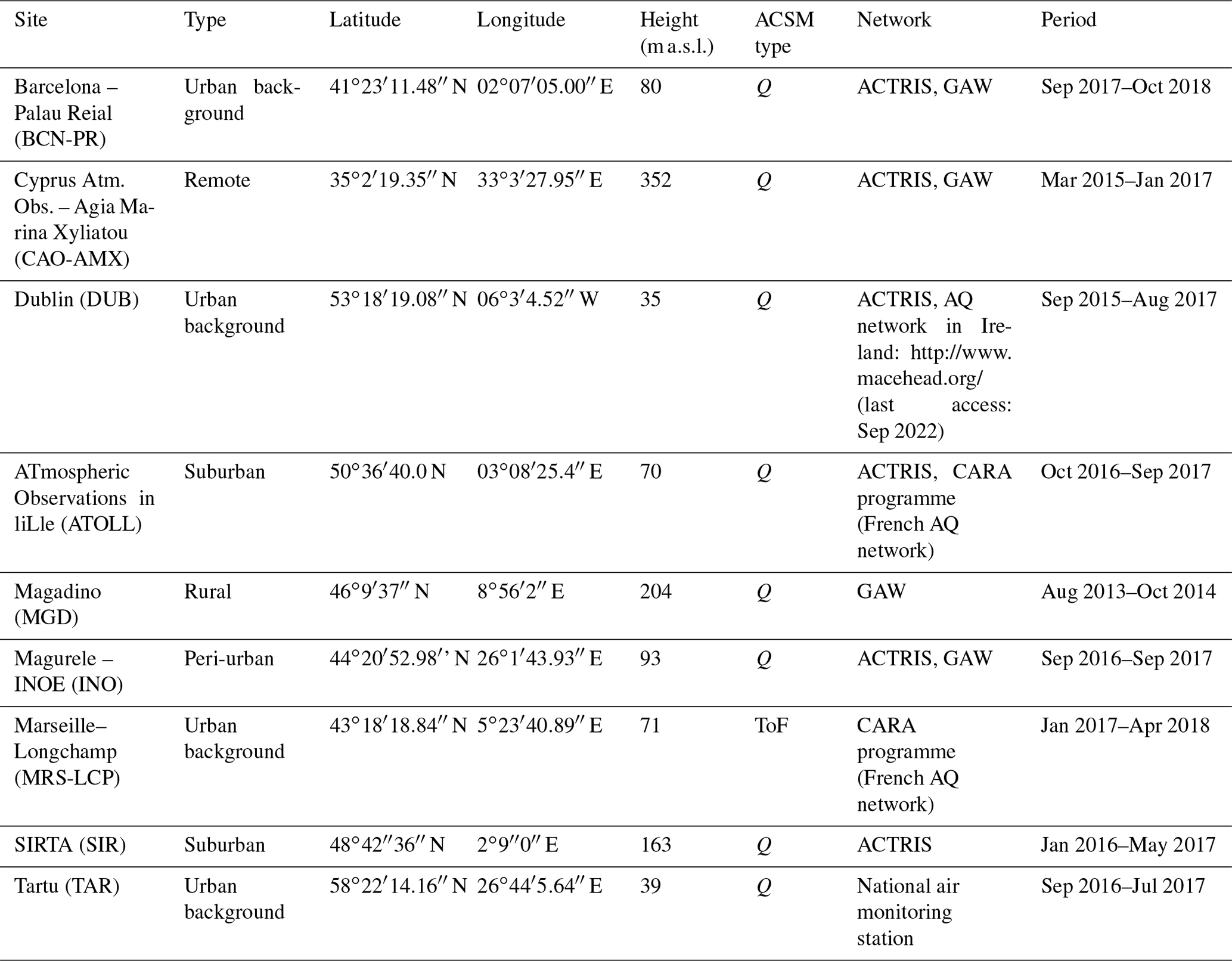
This study is one of the outcomes of the Chemical On-Line cOmpoSition and Source Apportionment of fine aerosoL (COLOSSAL) project (https://cost-colossal.eu/, last access: 14 September 2022) supported by the COST programme and based on measurements performed within the ACTRIS network. It is closely related to the overview study of Chen et al. (2022), in which 22 more-than-one-year-long PMF datasets were joined for a rolling PMF intercomparison. Participants of the WG2 of the COST COLOSSAL Action contributed to the preparation of a protocol for SA, with the purpose of homogenising the PMF application (Chen et al., 2022). A total of 9 of the 22 datasets from that study, whose main characteristics can be found in Table 1, were also provided for this rolling–seasonal comparison. Some of them contain site-specific sources related to instrument artefacts or proximity to pollution hotspots. The factors identified at all sites are hydrocarbon-like OA (HOA), biomass burning OA (BBOA, except for the Dublin site), less-oxidised oxygenated OA (LO-OOA), more-oxidised oxygenated OA (MO-OOA), and oxygenated OA (OOA), which represents the sum of LO-OOA and MO-OOA. Other factors are only present at one or two sites: cooking-like OA (COA; in Barcelona–Palau Reial and Marseille–Longchamp); 58-related OA (58-OA; in Magadino); shipping and industry OA (SHINDOA; in Marseille–Longchamp); wood combustion, coal combustion, and peat combustion OA (WCOA, CCOA, PCOA, respectively; in Dublin). The 58-related OA, as explained in Chen et al. (2021), is a factor dominated by nitrogen fragments ($m/z$ 58, $m/z$ 84, $m/z$ 94) that appeared as an artefact after the filament replacement in that instrument.

Table 1 Participant sites.

All data presented in the multi-site intercomparison were obtained from ACSMs, which use a mass spectrometer to measure the composition of non-refractory submicron particulate matter (NR-PM₁) in near-real time. It works at a lower mass-to-charge resolution, but it is more robust compared to the aerosol mass spectrometer (AMS, Aerodyne Research Inc, Billerica, MA, USA), allowing for long-term deployment. Both quadrupole (Q-ACSM) and time-of-flight (ToF-ACSM) ACSMs were used, further described respectively in Fröhlich et al. (2013) and Ng et al. (2011a). The resolution of ToF-ACSM datasets (10 min) was averaged to 30 min (resolution of the Q-ACSM) to have harmonised timestamps. The analysis software (version 1.6.1.1 for Q-ACSM and version 2.3.9 for ToF-ACSM), implemented in Igor Pro (WaveMetrics, Inc.), was provided by Aerodyne Research Inc. The treatment of the multi-site ACSM data to generate PMF input matrices is summarised in Table S1 in the Supplement, and more details can be found in the publications cited therein.

Ancillary measurements consisted of (i) SO${}_{\mathrm{4}}^{\mathrm{2}-}$, NO${}_{\mathrm{3}}^{-}$, NH${}_{\mathrm{4}}^{+}$, and Cl⁻ measurements from ACSM; (ii) black carbon (BC) from the filter-based absorption photometer AE33 from Magee Scientific (Drinovec et al., 2015), except for those from the Cyprus Atmospheric Observatory – Agia Marina Xyliatou and Magadino, in which the AE31 was used; BC concentrations were differentiated according to their main sources into fossil fuel (BC_ff) and wood burning (BC_wb) BC by applying the Sandradewi model (Sandradewi et al., 2008); (iii) NO_X concentrations; (iv) ultra-fine particles (range 20–1000 nm) at the Marseille–Longchamp site. Details on the complementary instrumentation at each site can be found in Table S2.

2.2 Synthetic dataset

Although the principal aim of this article is to inspect the differences in the methods amongst these European sites, a synthetic dataset comparison was first tackled. The main advantage of this procedure is that it allows the real-world environmental measurements already classified in OA sources to be mimicked so that PMF results can be compared with the incoming synthetic data. We created a synthetic dataset that mimics OA mass spectral analyses of a ToF-ACSM in Zurich. For that purpose, we used source-specific OA mass spectra retrieved from the AMS spectral database (Crippa et al., 2013; Ng et al., 2011b; Ulbrich et al., 2009) and OA source concentration time series generated by the air quality model CAMx (Comprehensive Air Quality Model with Extensions) previously published by Jiang et al. (2019). Details are described in Sect. S1. The dataset used to calculate the error matrix is that from the Zurich site, which ranges from February 2011 until December 2011. Hence, the same CAMx outcoming time series period was used to generate the concentration matrix. The represented OA sources are HOA, BBOA, SOA from biogenic emissions (SOA_bio), SOA from biomass burning (SOA_bb), and SOA from traffic and other anthropogenic sources (SOA_tr).

The first step for the synthetic dataset creation was to select p (number of factors), POA, and SOA spectral profiles from the high-resolution AMS spectral database (Crippa et al., 2013; Ng et al., 2010; Ulbrich et al., 2009) and to multiply them by the time series of the same sources from the model output. The error matrix was generated following the same steps as for real-world data, and real-world parameters were used as detailed in the Supplement. For this purpose, the dataset used is that from the Zurich site, which ranges from February 2011 until December 2011. Hence, the same CAMx outcoming time series period was used to generate the concentration matrix. Gaussian noise was subsequently added to the outcoming matrix. The resulting matrices were used as rolling and seasonal PMF input. Before the comparison to the original factors, several tests, as in the multi-site comparison, were performed to check the quality of the output; these tests included the mass closure test and the scaled residuals profile revision.

2.3 Positive matrix factorisation

The positive matrix factorisation model (Paatero and Tapper, 1994) describes the measured matrix X of n timestamps and m variables as a product of two matrices, G and F, plus a residual matrix E for a given number of factors p:

$$\begin{array}{}\text{(1)}& x_{ij}={\sum }_{i,j}^{n,m}{g}_{ik}\cdot f_{kj}+e_{ij}.\end{array}$$

The matrices G and F can be randomly initialised with a priori information. The model then iterates until the quantity

$$\begin{array}{}\text{(2)}& Q={\sum }_{i=\mathrm{1}}^n{\sum }_{j=\mathrm{1}}^m({\displaystyle \frac{e_{ij}}{{\mathit{\sigma }}_{ij}}}{)}^{\mathrm{2}},\end{array}$$

where σ_ij represents the uncertainties of the input matrix X, is minimised with respect to all model variables.

The use of a priori information reduces the rotational ambiguity of the model, consisting of a degeneration of solutions associated with a given Q value (Canonaco et al., 2013), and it is usually done from the a-value approach. This consists of initialising F (or G) with reference profiles (or time series) and multiplying them by the percentage of variation a, a∈ [0,1], where 0 and 1 would represent total constraint and freedom, respectively. The Source Finder (SoFi Pro, versions 6.8 and 8.04, Datalystica Ltd., Villigen, Switzerland) applies this algorithm through the multi-linear engine 2 (ME-2) (Paatero, 1999) within the Igor Pro software environment (Wavemetrics, Inc., Portland, OR, USA). SoFi is also a powerful software package for preparing the rolling conditions for the input matrices prior to the PMF algorithm and post-processing the outcomes afterwards.

2.3.1 Seasonal PMF

In order to apply seasonal PMF, the input matrix is divided into season-long submatrices, and PMF is applied independently, adjusting the number of necessary factors to the requirements of each subperiod. In order to reach an environmentally reasonable local Q minimum, the implementation of constraints on primary organic aerosol(POA) factors has been performed according to the COLOSSAL guidelines for source apportionment (COLOSSAL, COST Action CA16109, 2019) and the protocol from Chen et al. (2022). After unconstrained results exploration, which allowed for some marker identification, constraints based on the a-value approach were applied to primary OA factors. The systematic exploration of the a-value space has been performed for each season, with the aim of determining the combination of a values that maximises the correlations between factors and external correlations and represents an environmentally reasonable OA explanation, hereafter referred to as the base-case solution. The random a-value ranges and the reference profiles employed can be found in Tables S1 and S3a.

With respect to the synthetic dataset, the 11 months from 2011 data were split into three periods (and not four seasons to avoid running PMF over too short periods): February–May, June–August, and September–December. The real-world Marseille dataset also used the co-located SO₂ time series to force an industry + shipping factor to emerge, as reported in previous studies (Bozzetti et al., 2017; El Haddad et al., 2013). The seasonal averaging of the remaining runs were complemented by bootstrapping to estimate the statistical error of the solution.

Bootstrapping (Efron, 1979) the seasonal PMF input together with random a-value resampling allows for a statistical and rotational uncertainty assessment. The application of a criteria-based selection, which will be deeply explained in Sect. 2.3.2, was also used to discard those runs that did not comply with the user-defined standards. The outcome of this technique consists of p (number of factors) mass spectra and time series, including their uncertainty assessment, combined season-wise together to obtain period-long OA sources. This might lead to possible factor discontinuity. Moreover, from this approach, source fingerprints are static throughout a whole season and cannot adapt to the OA processes of lifetimes below a meteorological season (i.e. 90 d) but can nevertheless evolve from one season to another.

2.3.2 Rolling PMF

Rolling PMF runs the model on subsets of the input matrix with a user-defined (window) length in days. Then, the window is shifted by a number of days (also chosen by the user), and PMF is applied again (Parworth et al., 2015). Consequently, many PMF runs are performed in each window length period, so in the post-analysis, one can automatically discard the runs that do not meet certain user-defined criteria (Canonaco et al., 2015). To select the most environmentally reasonable runs, the remaining solutions are averaged to generate the final solution, which will be provided with statistical and rotational uncertainties based on random input resampling (bootstrap) and random a-value resampling, respectively.

A length of 14 d and a shift of 1 d were used in the current study for the synthetic dataset and for 7 out of the 9 datasets, which is a good compromise between $Q/Q_{\exp }$ values and the percentage of modelled points, as suggested in Canonaco et al. (2021). Window lengths of 28 d were also assessed, but the correlations to ancillary measurements deteriorated in most of the cases. Exceptions to this rule were the SIRTA and Tartu sites, for which the 28 d window offered better correlations. These window lengths are consistent with the life cycle lengths of atmospheric aerosols (Textor et al., 2006), and their outcomes do not differ significantly. The application of constraints in PMF, as advised in the protocols, consists of setting random a values within a reasonable range and accepting only the runs that comply with the criteria. This procedure will lead to the selection of a values that induce more environmentally reasonable solutions and whose average will provide the final number. In some cases, the reference profiles used in rolling PMF are those from the seasonal solution, as the protocol is flexible regarding this choice. However, this constraint can have an impact on the solution, and in order to identify its implications, the profiles used in each case are detailed in Tables S1 and S3a.

A criteria-based selection was developed to automatically inspect the large number of PMF runs provided by the rolling method (Canonaco et al., 2021). This consists of the application of certain criteria to be fulfilled by the PMF outcoming factors. The acceptance or rejection of a run can be dictated by the thresholds retrieved from bootstrapped seasonal solutions or, more advisably, from a double-tailed Welch's t-test hypothesis evaluation with p values (Chen et al., 2021) chosen by the user (not exceeding 0.05). This procedure allows for factor discontinuity, as one can run PMF for two consecutive numbers of factors and choose a certain criterion upon which to select one more (or less) factor depending on the outbreak or vanishing of a factor marker. The list of criteria is specified in Table S3b for the synthetic dataset and in the respective publications for each real-world site.

2.4 SA procedure and dataset homogenisation

A method to compare source apportionment performance, analogous to Belis et al. (2015) while adjusted for our specificities, was developed in this study. The first step consisted of preliminary checks, in which the minimum requirements for solution acceptance, such as the mass closure and reasonability of profiles, must be satisfied. Secondly, the characterisation of discrepancies between methods was addressed in order to confirm the presence or absence of significant differences between rolling and seasonal PMF. The decision of which method was more suitable for certain dataset particularities was a posteriori based on the quantification of the performance goodness of both methods by means of correlation to external measurements and residual analysis. This flow process was applied to both the multi-site analysis and the synthetic dataset.

All the participants of the multi-site comparison applied the SA protocol to their own datasets, benefiting from the expertise in the previous OA SA studies at their sites. The analysis of the differences between source contribution estimates by both methods was performed for each site individually and overall. The similarity of the time series from one method to the other was assessed not only for each whole dataset but also in a “rolling” fashion, that is to say, by calculating some metrics on the windows of a given number of days with 1 d shifts between windows. This approach allowed for the identification of significant discrepancies between both approaches for the set PMF window lengths (14 d for rolling, 90 d for seasonal), a feature that was not evident in the whole long-term time series. It also enabled the watching of intra-daily differences by setting period lengths of 1 d.

A detailed study of model residuals was also beneficial to quantify the accuracy of each technique's performance. Scaled residuals represent the model error (e_ij) normalised by the uncertainty matrix (σ_ij):

$$\begin{array}{}\text{(3)}& \mathrm{Scaled}{\mathrm{residuals}}_{ij}={\displaystyle \frac{e_{ij}}{{\mathit{\sigma }}_{ij}}}.\end{array}$$

Their i,j sum has been reported in Paatero and Hopke (2003) to describe a unimodal histogram within a ±3 range under good model performance conditions. The output Q quantity has been compared in both a raw and normalised way. This normalisation aims to deprive the impact of the degrees of freedom that normally depend on the input size and on the number of factors, hence computing the quantity $Q/Q_{\exp }$, where

$$\begin{array}{}\text{(4)}& Q_{\exp }=m\cdot n-p\cdot (m+n).\end{array}$$

Then, various PMF runs can be compared in a more fundamental way. The expressions used for the normalisation arrangement have to be adapted to the particular degrees of freedom of each method:

$$\begin{array}{}\text{(5)}& {\left({\displaystyle \frac{Q}{Q\mathit{\_}\exp }}\right)}_{\mathrm{Rolling}}={\displaystyle \frac{Q}{m\cdot n-p\cdot (n+m\cdot n_{\mathrm{14}})}},\end{array}$$

$$\begin{array}{}\text{(6)}& {\left({\displaystyle \frac{Q}{Q_{\exp }}}\right)}_{\mathrm{Seasonal}}={\displaystyle \frac{Q}{m\cdot n-\cdot p\cdot (n+m\cdot n_{\mathrm{90}})}}.\end{array}$$

The parameters n_14 d and n_90 d refer to the number of periods throughout the dataset of 14 and 90 d, respectively.

For the synthetic dataset, the comparison between methods had to consider the error of each. For this purpose, the metric presented in Belis et al. (2015), the uncertainty-normalised root-mean-squared error (RMSE_u) was used:

$$\begin{array}{}\text{(7)}& {\mathrm{RMSE}}_u={\displaystyle \frac{\sqrt{\frac{\mathrm{1}}{n}{\sum }_{i=\mathrm{1}}^n{\left(m_i-r_i\right)}^{\mathrm{2}}}}{\mathrm{2}u}}.\end{array}$$

In this expression, m represents the modelled values, r the reference values, and u the mean uncertainty of the model.

3 Results and discussion

3.1 Synthetic dataset

This section aims to assess the quality of the outcomes of the rolling and seasonal PMF methods. Relying on synthetic ToF-ACSM data offers the opportunity to compare the PMF outputs to the truth, which is not available for real-world measurements. We focus here on the OA sources' (factors') mean concentration and their temporal variability as well as the mean chemical composition and their temporal variability.

Regarding the OA apportionment vs. the input OA scatterplot, Table S4 presents the fitting coefficients for several resolutions, with no substantial difference between methods. Figure 1 shows the relative factor contributions to the apportioned OA for both methods. The POA factors do not differ substantially between the SA methods, but they are underestimated with respect to the truth (25 % of OA in rolling and seasonal, 35 % in truth). Also, whilst the LO-OOA-to-MO-OOA ratio is nearly 1 in the rolling case, it presents a much fresher secondary aerosol for the seasonal (1.5). Compared to the truth, PMF using a priori information on POA's chemical composition (HOA, BBOA) underestimates POA and overestimates SOA.

Figure 1 OA apportionment results for rolling and seasonal methods and truth output.

Figure 2 presents the time series, diel cycles of the truth, and rolling and seasonal methods as well as the scatter plots between the corresponding PMF time series. In time series and diel plots, it is noticeable that SOA is overestimated by PMF at the expense of POA (Fig. 2c). Squared Pearson correlation coefficients and slopes were similar for both rolling and seasonal, respectively, for HOA (0.89, 0.88) and OOA (0.95, 0.97) but not for BBOA, which seasonal resolves better (0.55, 0.72). Welch's t tests between rolling and seasonal time series rejected the similarity of all factors' concentrations. This test, applied to both methods against the truth, also rejected the hypothesis of significantly similar means, discarding a good method representation of truth results. This could be explained by the fact that truth profiles are static, and the methods were trying to adjust to moving fingerprints, and the anchor profiles might have influenced the results. For rolling and seasonal PMF results, the uncertainty-biased RMSE (RMSEu, Eq. 7) values are 1.10, 0.90 for HOA; 0.95, 1.98 for BBOA; and 0.05, 0.33 for SOA, respectively. Values under 1 represent values within the range of PMF uncertainty and are therefore acceptable values, which is the case for all except the rolling HOA and seasonal BBOA. These exclusions could be explained by two, non-exclusive hypotheses: (i) the dissimilarity between methods and truth is large; and (ii) the uncertainties of the methods might be underestimated. In all cases except for HOA, seasonal presents higher RMSEu and therefore a worse fit to the truth. Besides, the statistical Welch's t test was performed on the synthetic dataset PMF results, testing the null hypothesis of statistically similar means with different variances.

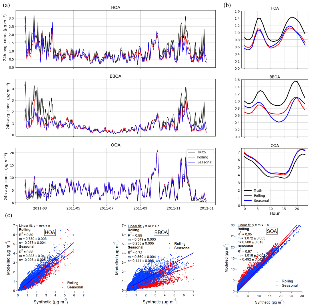
Figure 2 Rolling, seasonal, and truth (synthetic dataset original values) (a) time series (in hourly averages for the sake of clarity), (b) diel profiles, and (c) scatter plots.

The difference in the Pearson squared correlation coefficients between factors and their potential markers is shown as a histogram in Fig. S1 for each of the methods. The truth results show the worst correlation with ancillary measurements compared to modelled PMF. Rolling and seasonal results are very similar, although these correlations seem greater for rolling POA factors and for seasonal SOA factors. Slightly higher correlation coefficients were found for rolling in transition periods (i.e. ±7 d before and after the change of seasons): 0.88 and 0.77 for HOA vs. BC; 0.74 and 0.65 for HOA vs. NO_X; 0.52 and 0.52 for OOA vs. NH₄; and 0.07 and 0.07 for MO-OOA vs. SO₄.

Profiles (Fig. 3a) did not show remarkable discrepancies between PMF methods, but nonetheless, these could be noticed when compared to the truth profiles. However, the cosine similarity method revealed high similarity of both methods to synthetic profiles (1.00 and 1.00 for HOA, 0.91 and 0.91 for BBOA, and 1.00 and 1.00 for SOA for rolling and seasonal PMF, respectively). However, it is noteworthy that both HOA's and BBOA's chemical compositions were constrained. Model HOA profiles were very similar to the truth, except for the lower $m/z$ 44 and higher $m/z$ 57 of the truth, and other HOA markers regarding models. Modelled BBOA presented significant differences between the truth and modelled profiles; the truth profiles contained a lower $m/z$ 44-to-$m/z$ 43 ratio, the lower influence of HOA markers, and much higher $m/z$ 60 and $m/z$ 73 BBOA tracers. Hence, modelled BBOA contained a higher proportion of other OA factor markers and lower of their own, meaning modelled profiles might have resulted in less cleanliness than the true ones. SOA PMF modelled profiles contained lower $m/z$ 43 and $m/z$ 44 than the truth profiles, although the rest remained very alike. In short, PMF results present a BBOA factor with more SOA and HOA influence as the main profile. The underestimation of POA is therefore understood to be due to a poorer modelisation of the key source identifiers, leading to a less pure profile and hence, a lower mass apportionment compared to truth.

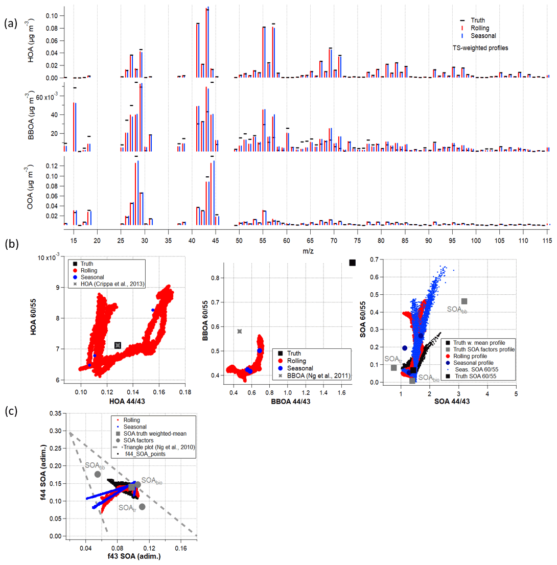
Figure 3 Synthetic dataset solution (a) profiles; (b) time-dependent profile variability of ratios $\mathrm{60}/\mathrm{55}$ vs. $\mathrm{44}/\mathrm{43}$; (c) triangle plot of f44 vs. f43 for rolling PMF (red), seasonal PMF (blue), and truth (black).

The influence of reference profile constraints might have enhanced the misattribution of the profiles – for example, imposing $m/z$ 44-to-$m/z$ 43 ratios led to a significant difference in the degree of oxidation solution with respect to truth. Nevertheless, constraining profiles has provided more accurate solutions than unconstrained setups, as shown in Fig. S2. These plots show how seasonal constrained PMF launches always present higher similarity to truth in terms of key ions ratios. Moreover, OA sources of unanchored runs were less robust due to lower reproducibility along the accumulation of runs. By extension, rolling results are expected to reproduce the same results, as it has been proven that both techniques' outcomes converge sufficiently.

The adaptability of the models can be assessed from Fig. 3b, where the $\mathrm{60}/\mathrm{55}$ vs. $\mathrm{44}/\mathrm{43}$ (which are proxies for the BBOA–HOA differentiation and the SOA oxidation, respectively) is plotted for the truth and for both methods. Here we use $m/z$ 55, since it is known to be a key marker for HOA. Rolling is shown to be a continuous time series, as the profiles for this method are time dependent, whilst the ratios for seasonal only vary from season to season. In HOA, the modelled points circle the actual truth and anchor profile points (which are similar or equal), but this is not the case for BBOA, in which the rolling and seasonal points are near the anchor profile but distant from the truth. This implies that the anchor profile, which was selected ignoring the truth profile characteristics, plays an important role in terms of adaptability to the actual solution. Overall, even for OA sources with nominally constant chemical composition (here HOA, BBOA), the factors resolved by PMF exhibit a varying chemical composition. Therefore, caution is required in interpreting the variability in sources of chemical variability resolved by rolling PMF. Oppositely, the SOA profiles, as they were unconstrained, can be compared more fairly. Both the rolling and seasonal dots are within the truth markers, except for some points of high $\mathrm{60}/\mathrm{55}$, for which the highest disparity to truth is found for seasonal. This suggests a poorer PMF OOAs chemical composition profile apportionment, which in turn, might be influenced by the POA anchoring deficiencies.

The benefits of the continuity of the rolling profiles are reflected in time series, as can be seen in Fig. 3c, in which the behaviour of seasonal points is unrealistically drastic depending on the season. The profile adaptability of the rolling method represents a more resolute approach to positively representing the truth. Contrarily, the seasonal approach – although it can be plotted for each timestamp, as SOA is the sum of two OOAs – can only vary in lines of an equal $\mathrm{44}/\mathrm{43}$ ratio, as the profiles are constant all through a season. In short, it can be stated that, as opposed to seasonal PMF or in general batch-wise PMF analysis, rolling PMF offers the potential to interpret changes (e.g. seasonal) in an OA sources' chemical composition, but the anchor profile selection has been shown to generate significant discrepancies when compared to the truth for both methods, requiring caution in interpreting such variability.

The SA method used has a severe impact on model-scaled residuals. Figure S3a shows the histogram of the scaled residuals for all the resolutions. In all cases, the rolling PMF histogram is significantly sharper, more centred to zero. Also, the same effect is visible in the transition periods (Fig. S3b). Regarding Q values, the rolling value (3 838 356) is lower than the seasonal value (24 665 377), as expected, due to the higher extent of degrees of freedom of the former method. $Q/Q_{\exp }$ values, computed from Eqs. (5) and (6), are 7.08 and 37.58, respectively, for rolling and seasonal PMF. The fact that, when normalising by the model-specific degrees of freedom, the $Q/Q_{\exp }$ is lower for rolling than for seasonal leads to the conclusion that the minimisation of uncertainty-weighted errors is better achieved by the rolling method.

3.2 Multi-site comparison

3.2.1 Preliminary tests

Preliminary tests were performed to check the consistency of the reported results as well as the actual difference between the methods reported. An important performance metric is the closure of the OA mass – that is to say, the difference between the sum of all OA factor concentrations vs. the input mass. Table S4 provides the fit statistics of the input OA vs. the outcome OA for all the sites and four different time spans (the whole period, a season, a fortnight, and a day). All squared correlation coefficients are higher than 0.88, and slopes are within the 0.92–1.09 range. This ensures the quality of the PMF performance at all time resolutions and for both methods. A closer inspection of the table shows slightly higher correlation coefficients and slopes closer to 1 for rolling.

In order to confirm or reject the existence of systematic disparity between both methods, a two-tailed Welch's t test was performed under the null hypothesis of the time series having statistically similar expected values. In Table S5, all cells marked represent the runs that reject the null hypothesis, i.e. for which the factors retrieved from rolling and seasonal are not statistically equal (p values over 0.05). The row “all” refers to the concatenation of all the dataset time series. Apportioned OA presents the highest acceptance of the hypothesis rate, implying that the global apportionment means are not significantly different. The factors with higher rejection rates are LO-OOA, MO-OOA, and HOA, in this order. OOA factors, as they are unconstrained, might be rather sensitive to source outbreaks or variations, which could have been caught or not by one model, although their sum (OOA) remains coherent. Period-long figures get the highest rejection rates, which decay rapidly from lower to higher resolutions, meaning the seasonal and fortnightly averages are still high despite their rapid resolution; on the other hand, for the daily resolution, this rate is very low. This fact highlights that the methods present significant differences with regard to means in intermediate resolutions.

Figure S4 compares the relative difference of the rolling minus seasonal concentrations for each factor in the all-sites ensemble. The factors with higher errors are MO-OOA and LO-OOA, tilted to positive values – that is, resulting in higher concentrations for rolling. This is probably related to the lack of anchors, which promotes higher freedom and hence, higher difference between methods. Also, BBOA presents significant positive whiskers, but as mean concentrations in Fig. 1 are equal, we suspect these are linked to sporadic high concentration outbreaks, which might only have been caught by the rolling method. Besides, the other factors are not significantly different from zero.

The pie charts in Fig. 4 show the amount of mass apportioned by the main OA sources in all datasets. These pies do not account for site-specific sources; they present the relative contribution of the all-sites ones scaled to account for the 360 degrees. OA is mainly driven by secondary organic aerosols in both cases, although the ratio of fresh-to-aged aerosol contributions – that is, LO-OOA over MO-OOA – is much higher for rolling (0.62) than for seasonal (0.54). The ratio of POA over SOA is higher for seasonal than for rolling (0.58 and 0.37, respectively), and the ratio of BBOA over HOA is considerably different (1.17 and 1.45, respectively). The fact that wood burning BC exceeds fossil fuel BC is consistent with the average ratio of 3.1 for BC_wb and BC_ff, implying that PMF reproduces this relation. Hence, rolling describes a more oxidised SOA, which is less prevailing than that of seasonal. In both, POA is governed by the biomass burning OA. Figure S5 shows the individual apportionment pies, in which the same trends can be generally recognised. In general terms, these results do not coincide with the ones from the synthetic dataset, in which the POA/SOA and LO-OOA/MO-OOA ratios were, respectively, equal and higher for rolling.

Figure 4 Pie charts of the mean concentrations of the main factors for the ensemble of all sites.

Figure 5 shows both the monthly and diel cycles of the rolling minus seasonal concentrations of the ensemble of sites for the main factors. In general terms, the intra-year variation is not remarkable, as all the boxes are mainly crossing the zero line. Besides, the differences between mean and median could indicate the adaptability to spiky events. The fact that HOA and BBOA are remarkably different throughout the whole period coincides with the aforementioned Welch's t tests. Moreover, the mean for HOA in January and December and for BBOA in July and August are positively set beyond the boxes, which could imply that the most extreme events are better captured by the rolling. This fact reinforces the hypothesis of a more precise capture of intra-month events. SOA factors present fewer clear trends, although an alternate sign between warm and cold months can be recognised. Figure S6 depicts the behaviour of the remaining factors, which are nearly zero except for 58-OA, which is significantly negative in summer, and SHINDOA, which alternates from positive to negative from summer to winter. In the case of 58-OA, this indicates a summertime under- or overestimation of one of the methods, and for the SHINDOA, a differing capturability of events along the year.

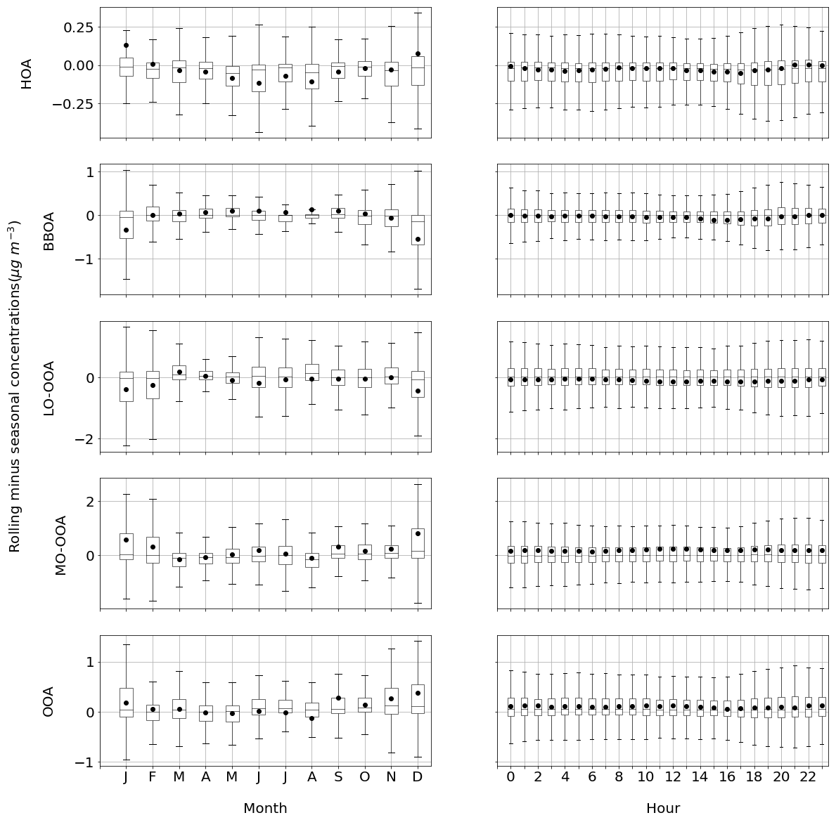
Figure 5 Boxplots of rolling minus seasonal factor absolute concentrations (in µg m⁻³) per month and hour. Boxes show the Q1–Q3 range with the median (horizontal line) and the average (full circles); whiskers extend up to the range of the data.

Regarding diel cycles (Fig. 5), the differences are evident in HOA and BBOA at night, implying that this is where the mixing between POA sources is aggravated. The SOA factors reveal that one of the methods overestimates the other throughout the daily cycle: rolling is greater for MO-OOA and OOA and lower for LO-OOA. Whilst these differences do not have an impact on the Welch's t test for LO-OOA, they do for the rest, even for HOA, for which they are not very uneven, probably due to the compensation of differences while averaging. Figure S6 shows similar behaviour for both methods in all the factors except for the WCOA, PCOA, and CCOA, which present higher differences at night. Seasonal concentrations, though, are remarkably higher for 58-OA throughout the period or daily cycle, somewhat superior in the COA 8h peak, and inferior in the SHINDOA afternoon. While these results do not have an impact on the p value for the Barcelona–Palau Reial and Magadino sites, it does for the Marseille–Longchamp site.

3.2.2 PMF goodness evaluation

Correlation with ancillary measurements

In order to assess the quality of each PMF method outcome, the correlation of factors with their potential markers was monitored from a single and global perspective. The pairs of variables compared were: HOA and BC_ff, HOA and NO_x, BBOA and BC_wb, MO-OOA and SO${}_{\mathrm{4}}^{\mathrm{2}-}$, and OOA and NH${}_{\mathrm{4}}^{+}$. SHINDOA was compared to ultrafine particles with diameters of 10–20 nm coming from shipping or industry, differentiated according to Chazeau et al. (2021) and Rodríguez and Cuevas (2007). The correlation of LO-OOA vs. NO${}_{\mathrm{3}}^{-}$ has been excluded in this study due to the plentiful sources of NO${}_{\mathrm{3}}^{-}$; besides, organonitrates would hamper the traceability of LO-OOA from this compound. This analysis has not been extended for the rest of the OA sources due to the lack of appropriate tracers available.

Figure 6 presents the Pearson squared correlation coefficient for all the pairs of markers and factors retrieved from rolling and seasonal PMF. Even though these marker time series are not deprived of errors, the hypothesis is that better agreement leads to better adaptation of the model to the OA source emitting these tracers. Overall, the rolling boxes are centred to higher correlation values than the seasonal ones, but their whiskers always reach the maximum value of 1 in both cases. The difference between methods is small, since medians do not differ by more than 0.05; however, the seasonal performance underscores these correlations slightly. This finding would support the hypothesis of the superior performance of the rolling, although HOA is evenly characterised in both methods, which is consistent with the great similarity in the apportionment of OA shown in Fig. 4. The histogram for the difference of Pearson squared correlation coefficients is plotted as a histogram for all sites in Fig. S7. Positivity in this graph reflects better rolling results matched with co-located measurements, and the histogram spreads the range of correlations. The amount of shoulders in the right half of these histograms is higher than those in the left, which implies systematic improvement of the rolling method with respect to seasonal in terms of correlation with ancillary measurements.

Periods of transition from one season to another are strategically relevant for this comparison, since the seasonal method, due to its profile staticity definition, could yield to discontinuities in the time series of the different components. The change of OA factors spectra for rolling is smooth; therefore, no abrupt changes should be expected in the season edges. Moreover, the rolling technique is capable of introducing factors depending on criteria compliance; therefore, their concentration edges are not as sharp as they would be for the seasonal PMF. This is the case for BBOA appearance in the cold months in Barcelona–Palau Reial and Marseille–Longchamp, and the 58-OA outbreak after the Q-ACSM filament replacement in Magadino. From these premises, one could expect to find better correlation coefficients relating to factors and their markers for the rolling method, which could better represent these periods. Table S6 shows the correlation of the OA factors and their markers for these periods only, both for the rolling and seasonal PMF. In all cases, the differences between methods are not extensive. However, it can be seen how the “whole” dataset figures are always greater for rolling than for seasonal. This finding supports the conjecture that the seasonal method presents greater difficulty in representing the edges of the seasons. The relevance of this conclusion is to be considered especially in the datasets in which the number of days near season changes is important due to data gaps.

Model residuals

Figure 7 shows the normalised scaled residuals distribution for both methods in a concatenated dataset including all the sites. Given that the uncertainty matrix was the same for both techniques, scaled residuals reflect the capacity of each technique to apportion the quantity of OA most similar to that which was entered as input. Boxplots show a tendency towards negative values for both methods, implying a systematic bias towards the overestimation of the input matrices. Seasonal errors present a higher spread and lower mean and medians; hence, seasonal results are less accurate and precise than those from rolling, overall. However, the span of both distributions does not exceed the ±3σ threshold in any of the cases, meaning the results are acceptable for both techniques. Figure S8 shows the same plot for each of the participant sites. In general, the rolling histograms are more centred to zero, and their sharpness is higher with respect to seasonal distributions. An exception to this behaviour is Marseille–Longchamp, which presents negatively shifted distributions probably related to the model's difficulty in differentiating between BBOA and LO-OOA.

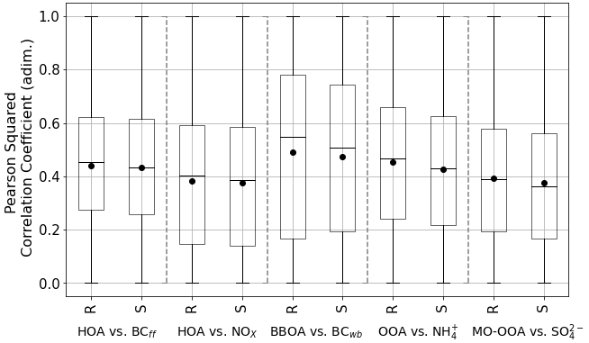
Figure 6 Rolling (R) and seasonal (S) boxplots of the Pearson squared correlation coefficient of each OA source with its respective markers for all sites.

Scaled residuals for the season transition periods are presented in Fig. S9. Both histograms extend largely beyond the (−3, 3) domain, implying that both methods struggle in this kind of period; however, the seasonal distribution of scaled residuals is much wider than that of rolling. Also, in the zoomed (−3, 3) range, seasonal results seem to present a wider distribution. Distribution shoulders are present in both – negative in rolling and positive in seasonal – indicating rolling overestimation and seasonal underestimation of input concentrations. These findings would imply that, even if the methods provide a substantial error in the transition periods, the rolling better captures the season change due to its profile adaptability.

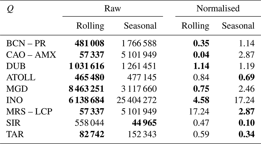
Regarding Q values, the differences between techniques are presented in Table 2. Unweighted Q values show a clear pattern on lower values for rolling PMF, except for one site. The SIRTA datasets were treated by two different users, which might have led to different PMF steps and unreliable results. The generally greater minimisation of Q performed by the rolling PMF method can be explained by the major quantity of runs performed compared to seasonal PMF because of the proper definition of the method. By depriving the Q of the degrees of freedom effect, as shown in Eqs. (5), (6), the minimisation of both methods is signified. The trend generally points to lower figures for the rolling method, but whilst the minimisation of the unweighted Q was an expected fact, the implicit error reduction cannot be ensured within a theoretical frame. However, the majority of sites (excluding the aforementioned SIRTA) show lower $Q/Q_{\exp }$ values for the rolling method.

Figure 7 Normalised scaled residuals histogram for both PMF techniques.

Table 2 $Q/Q_{\exp }$ values for rolling and seasonal solutions. Bold figures represent the lowest value in the rolling–seasonal comparison.

Adaptability tests

Adaptation tests were designed to inspect how much the methods comply with the input data. One of the main concerns to assess is the adaptability of the output profiles to short-lifetime events (order of magnitude of days), as it is the hypothesis onto which the rolling PMF is based. For this purpose, the check was based on the difference between main ion ratios, calculated from input values and the apportioned amounts of these ions by OOA factor profiles for both methods, e.g. ($m/z\mathrm{44}/m/z\mathrm{43}{)}_{\mathrm{input}}$ – OOA ($m/z\mathrm{44}/m/z\mathrm{43}$) Rolling or Seasonal. This can be seen in Fig. S10 in a time-series form for each site. Because $m/z\mathrm{44}$ and $m/z\mathrm{43}$ are also part of POA profiles, one should not expect to find a perfect match between the raw and the OOA profile ratios but rather a qualitative idea of how well the profiles adapt to the degree of aerosol ageing. In these plots, generally the rolling profile variation seems to adapt better than seasonal, which is a straight line along a season. Under the same logic, Fig. 8 shows the site histograms of the ($m/z\mathrm{44}/m/z\mathrm{43}{)}_{\mathrm{input}}$ – OOA ($m/z\mathrm{44}/m/z\mathrm{43}$) Rolling or Seasonal values only for periods around the change of season, which have been proven to be tricky for the PMF model.

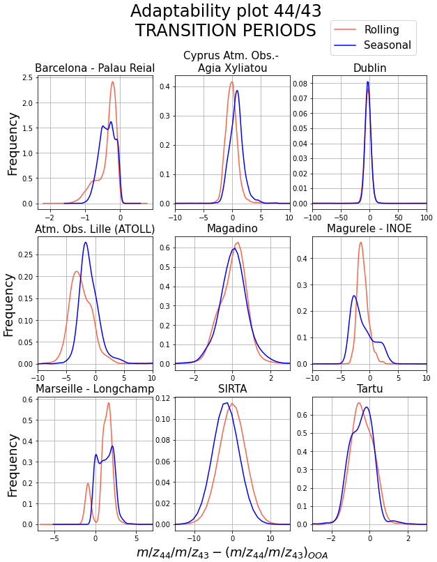
Figure 8 Kernel density estimation of the histograms of the subtraction of the $m/z$ 44-to-43 ratio from the raw (from input matrices) time series data minus the apportioned quantity in profiles. These plots only contain those time lapses among the change of season (transition periods).

Figure S9 shows, in general terms, how the rolling adapts to the main 44-to-43 trends, whilst seasonal can only present a single value for a whole season. Even though the rolling or seasonal SOA and the input time series are not expected to match perfectly, the main features of the variability are usually caught by the rolling. By taking a look only at the transition periods in Fig. 8, the tendency is that the difference between the input ratio and the rolling ratio is closer to zero or sharper around it than with seasonal. These qualitative appreciations bolster the aforementioned conclusion that rolling adapts the SOA profiles to specific singularities of the input time series, thus generating a more accurate solution.

4 Conclusions

The present study aimed at performing a comprehensive comparison between the two methodologies of fine organic aerosol (OA) source apportionment through the positive matrix factorisation (PMF) model: rolling and seasonal PMF.

The synthetic dataset rolling and seasonal outputs assessment has been rather fruitful for this comparison. The main highlight of this approach is that the modelled sources could be compared to the “truth” ones – that is, the OA sources chosen artificially during the dataset tailoring. Contrasting PMF results against the truth highlighted the model's overestimation of SOA and underestimation of POA (in the case of using a priori information on POA's chemical composition) for both rolling and seasonal and different degrees of SOA oxidation between methods. Nevertheless, the correlation of rolling and seasonal with the truth time series and profiles show very similar results in terms of concentrations. The temporal variability of OA sources' chemical composition has been shown to oscillate, even for POA components with temporally invariant chemical composition, and to be severely impacted by the selection of the profile anchors, as it differed significantly from the truth results when the anchor was significantly different to the truth profile. However, the use of profile constraints still provided solutions closer to the truth than unconstrained PMF. Besides, the rolling method has been proven to give a more sensitive representation of the continuous OA fingerprints variation. Scaled residuals minimisation also supported that the rolling solution was mathematically superior to seasonal.

The following multi-site comparison pretends to contrast both PMF methods in real-world datasets treated homogeneously under Chen et al.'s (2022) protocol to observe general performance trends. The rolling method generally presents a comparatively similar proportion of primary OA (POA) and a secondary OA (SOA) of a lower oxygenation degree, i.e. the ageing state. The double-tailed Welch's t test showed that the narrower the window of inspection, the higher the differences between factors retrieved from one method to the other. Moreover, towards weekly or daily periods, SOA factors differ more than POA factors. This fact is likely due to the absence of constraints for the SOA factors during PMF. Contrastingly, POA factors are more dissimilar period-wise. The ratio of BBOA to HOA differs considerably from rolling to seasonal (1.45 and 1.17, respectively) for the ensemble of sites, but in any case, it is over 1, as the ratio of BC_wb to BC_ff suggests.

In general terms, rolling results correlate better with ancillary measurements than those from seasonal for almost all of the considered external datasets at all sites. This is particularly true in the days surrounding the change of season, in which the seasonal profiles change drastically from one time point to the following. Model residuals also point to a better minimisation for the rolling PMF, although regarding scaled residuals, both methods comply with the (−3, 3) range advised by the protocol. The time series of key ions also quantitatively pointed to a better adequation of the rolling SOA profiles to the oxygenated OA key ions. Finally, the errors also proved to be more stable for the rolling method, while it should be noted that the individual sites' discrepancies from the overall trends have not been discussed in this study.

Overall, these results confirm the hypothesis that the rolling PMF can be considered more accurate and precise, globally, than the seasonal one, although both meet the standards of quality required by the source apportionment protocol. Moreover, the rolling method was already recognised to involve less user subjectivity and computational time as well as being more suitable for long-term and evolving SA analysis, such as semi-automated online SA. This study, therefore, promotes the acceptance of this novel rolling method as an improved approach suitable for source apportionment studies. An additional conclusion stemming from this comparison is that the selection of anchor profiles strongly influence the OA factors, so local reference profiles are encouraged to minimise this impact.