Image muting of mixed precipitation to improve identification of regions of heavy snow in radar data

In winter storms, enhanced radar reflectivity is often associated with heavy snow. However, some higher reflectivities are the result of mixed precipitation including melting snow. The correlation coefficient (a dual-polarization radar variable) can identify regions of mixed precipitation, but this information is usually presented separately from reflectivity. Especially under time pressure, radar data users can mistake regions of mixed precipitation for heavy snow because of the high cognitive load associated with comparing data in two fields while simultaneously attempting to discount a portion of the high reflectivity values. We developed an image muting method for regional radar maps that visually de-emphasizes the high reflectivity values associated with mixed precipitation. These image muted depictions of winter storm precipitation structures are useful for analyzing regions of heavy snow and monitoring real-time weather conditions.

1 Introduction

Weather radar data from ground-based scanning radars are crucial for monitoring the location, intensity, and evolution of storms. Winter storms in mid-latitude regions often contain subregions with rain, mixed precipitation, and snow that move and evolve over the storm lifetime (Schultz et al., 2019). Higher radar reflectivity values are generally associated with heavier precipitation. But the transition among rain, partially melted snow, and snow precipitation types creates a challenge when interpreting radar reflectivity because volumes with melting precipitation have higher reflectivities than volumes with the equivalent precipitation mass of only ice hydrometeors or only liquid hydrometeors (Vivekanandan et al., 1994; Straka et al., 2000; Rauber and Nesbitt, 2018).

In particular, the changes in phase from ice to partially melted ice and then to rain modify the dielectric constant of the particles so that volumes with the same precipitation mass per unit volume can have different reflectivity values (Battan, 1973). When analyzing banded snow features in winter storms, areas of mixed precipitation can be distracting and misleading (e.g., Picca et al., 2014. We define mixed precipitation as precipitation that includes combinations of rain or freezing rain, snow, sleet, and partially melted snow.

Regions of mixtures of precipitation types can be identified with the dual-polarization radar variable known as the correlation coefficient (ρ_HV) (Table 1; e.g., Vivekanandan et al., 1994; Straka et al., 2000; Kumjian, 2013a). The correlation coefficient is a statistical measure of how consistent the shapes and sizes of particles are within a radar resolution volume (Rauber and Nesbitt, 2018). This variable is insensitive to radar calibration and yields comparable values for the same set of hydrometeors across radar networks with identical hardware and signal processing methods. The correlation coefficient is approximately 1 in regions with single hydrometeor types (e.g., only rain or only snow) and decreases in regions where there is an increasing diversity of hydrometeor orientations and shapes (e.g., mixed precipitation such as rain with snow and/or partially melted ice) (Giangrande et al., 2008; Rauber and Nesbitt, 2018). Additionally, the correlation coefficient can have low values in various types of ground clutter and is used in identifying nonmeteorological echo (e.g., Zrnić et al., 2006; Alku et al., 2015; Kumjian, 2013b).

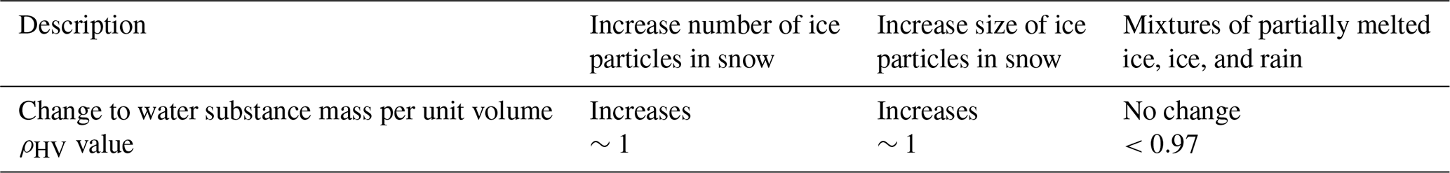
Table 1 Correlation coefficient values associated with physical mechanisms that increase radar reflectivities when Z>20 dBZ and other conditions are held constant.

Although the correlation coefficient is insensitive to radar power calibration, it does suffer from other data quality problems. Artificially lower ρ_HV values can occur along radials downrange of sharp gradients in differential phase (Ryzhkov, 2007). With increasing range from a radar, radar resolution volume size increases and signal-to-noise ratio (SNR) decreases. For example, near the melting layer, larger radar resolution volumes are more likely to have non-uniform beam filling than smaller radar resolution volumes. In theory, non-uniform beam filling of a radar resolution volume would tend to decrease the correlation coefficient (Ryzhkov, 2007). However, the current method used to compute the correlation coefficient in US NEXRAD operational radars yields increased values with decreasing SNR (Ivić, 2019). Unlike radars that transmit at horizontal and vertical polarizations, the NEXRAD radar transmits at a single polarization oriented at 45^∘, which reduces the overall sensitivity of the radar and under conditions with canted, oriented ice can reduce the correlation coefficient (Rauber and Nesbitt, 2018). In practice, the impact of SNR tends to be much more prevalent than non-uniform beam filling. This suggests that the SNR effect might mask most of the effects of non-uniform beam filling in NEXRAD correlation coefficient data quality. Dual polarization radar variable data quality problems are more pronounced when there are mismatched antenna patterns in the horizontal and vertical polarizations (Bringi and Chandrasekar, 2001), which are more common in operational radars than in research radars.

As reflectivity, the correlation coefficient, and hydrometeor types are usually presented as separate products (NOAA, 2017), someone wanting to discern regions of heavy snow versus mixed precipitation in a winter storm needs to toggle back and forth among different products or overlay them. Neural science studies show that switching between sources of information increases the cognitive load of a task (Sweller et al., 2011; Harrower, 2007). Keeping track of changing shapes of moving objects is particularly challenging (Suchow and Alvarez, 2011). Integrating related material and removing irrelevant material is essential for maximizing understanding and learning (Mayer and Moreno, 2003; Sweller et al., 2011; Harrower, 2007).

In order to reduce the cognitive load associated with analyzing precipitation structures in reflectivity, we propose a new visualization technique we refer to as “image muting”. Image muting aids interpretation of sequences of radar data in movie loops. We plot the reflectivities using a perceptually uniform, color-blind-friendly color scale and the subset of reflectivity values corresponding to mixed precipitation using a gray scale of matching perceptual lightness. This visualization does not remove areas of melting but rather “mutes” them, making the regions stand out less than the snow-only or rain-only portions of the storm. Work by Calvo et al. (2021) demonstrates how making small changes in climate visualizations can reduce the cognitive load and support analysis and potential decision making.

Our image-muting technique is described in detail in Sect. 2, and applications of our technique are presented in Sect. 4.

2 Methods

To demonstrate the methodology, we used Level II data from several National Weather Service (NWS) Next-Generation Radar (NEXRAD) network radars in the northeast United States (US) that were obtained from the NOAA Archive on Amazon Web Services (Ansari et al., 2018). Complete volume scans are available from each radar approximately every 5 to 10 min. This technique can be applied to any radar data set that has both reflectivity and correlation coefficient fields.

2.1 Regional mapping

We combine data from several radars to create regional radar maps utilizing functions in the open source Python Atmospheric Radiation Measurement (ARM) Radar Toolkit developed by the Department of Energy ARM Climate Research Facility (Py-ART; Helmus and Collis, 2016). We first extract the first 0.5^∘ elevation angle plan-position indicator (PPI) from each volume scan. We do not interpolate to a constant altitude in order to preserve as much fine-scale detail in the reflectivity and correlation coefficient structures as possible. We include only data within a range of 200 km of a radar as this is sufficient for combining data from multiple radars in much of the continental US without substantial gaps, and constrains the beam center to be at an altitude less than 4 km above radar level. The polar coordinate data from each individual radar are interpolated using Cressman weighting (Cressman, 1959) to a Cartesian grid covering our geographic region of interest. Before interpolating, we convert the reflectivity from units of dBZ to units of mm⁶ m⁻³ because interpolating in linear reflectivity units provides a more accurate representation of the polar data (Warren and Protat, 2019). We interpolate each polar radar object used in the regional map to the same Cartesian grid with 2 km grid spacing. For the northeast US regional maps shown in this paper, the regional grid is 1201 km ×1201 km. We convert the reflectivity back to dBZ after the interpolation step. Finally, to combine data from all the radars into a single object, we designate a “central radar” to which to stitch all the other radars. For storms in the northeast US, we use the Long Island, NY (KOKX) radar as the central radar. For each volume scan at KOKX, we find the closest time from the other radars (within 8 min). For grid points where coverage from adjacent radars overlaps, we use data from the radar with the maximum reflectivity value and its corresponding correlation coefficient value. Use of the maximum reflectivity value means adjacent points can be from 0.5^∘ elevation angles from different radars yielding discontinuities in an altitude of up to 4 km. As our main research application is identifying snow bands and lighter versus heavier regions of snow, having adjacent points not continuous in altitude was an acceptable trade off. Before plotting the fields, we despeckle the data to remove areas of echo that are less than 20 km².

2.2 Identification of mixed precipitation

In effect, we are implementing a hydrometeor identification for only mixed precipitation. We simplify the radar data visualization by choosing this one hydrometeor category to de-emphasize in the reflectivity field. We identify grid points where the hydrometeors are partially melted and/or mixed rain and snow, where the ρ_HV is below a threshold of 0.97, and where the reflectivity value is greater than or equal to 20 dBZ. We used 0.97 following Giangrande et al. (2008), who found that the correlation coefficient for dry snow exceeded this value. Adding the criterion of reflectivity ≥20 dBZ was essential in distinguishing regions of melting or mixed precipitation that could be confused with heavy snow from regions of light precipitation with noisy, unreliable ρ_HV values. The 0.97 ρ_HV and 20 dBZ thresholds are consistent with Griffin et al. (2020), who used ρ_HV to detect melting layers in radar data. We note that not all clutter points are removed in our regional maps, which can have low values of ρ_HV and may show up as stationary features in animations of image-muted maps.

Any method relying on a particular variable as input will not work well when there are data quality problems with that variable. Data quality problems with the correlation coefficient along radials downrange of sharp gradients in the differential phase will yield sporadic image-muted areas radial to the radar that will not move consistently with the advection of locally enhanced reflectivity bands within the storm. Regions of speckled image muting based on the method described here could either be a result of small spatial-scale variations in the melting of snow or noise in the correlation coefficient field related to low SNRs, which are more common at ranges further from the radar (Ivić, 2019).

The inputs and outputs for image muting from a coastal winter precipitation event on 7 February 2020 are shown in Fig. 1. Information from regional maps of the radar reflectivity field (Fig. 1a) and the correlation coefficient field (Fig. 1b) are combined. We show an intermediate stage (Fig. 1c) illustrating the pragmatic importance of using both the correlation coefficient and the reflectivity criteria. ρ_HV values ≤0.97 often occur toward the edges of the individual radar echo domains where the beam is $>\sim \mathrm{3}$ km altitude and in winter storms very likely to be only snow (green region in Fig. 1c). We infer that the reflectivity <20 dBZ is too low to reliably indicate mixed precipitation that can be mistaken for heavy snow. The areas in gray represent regions where the ρ_HV≤0.97 and the reflectivity is ≥20 dBZ, where melting is likely to be present and where we mute the reflectivity. Dark blue colors in Fig. 1c are where the correlation coefficient is >0.97, indicative of uniform precipitation types. The final image-muted reflectivity product (Fig. 1d) uses a gray scale to de-emphasize the subset of reflectivity values where it is likely to be mixed precipitation. This example shows two linear features in central New York that could be misinterpreted as purely snowbands when analyzing the reflectivity alone (white ovals in Fig. 1a). The animation of Fig. 1 (Animation-Figure-1 in the Video supplement) for the time period 12:00:00 to 15:00:00 UTC shows how the mixed precipitation region covers portions of the high reflectivity bands in Fig. 1a as the bands move eastward. The image-muted reflectivity helps users to focus on regions of the storm that are not affected by mixed precipitation. We experimented with trying to distinguish the rain-only from the snow-only regions but found that there was insufficient information in the dual-polarization radar variables to do this reliably without data on air temperature. Air mass and frontal boundaries can cause freezing level heights to vary sharply within winter storms, unlike warm-season precipitation.

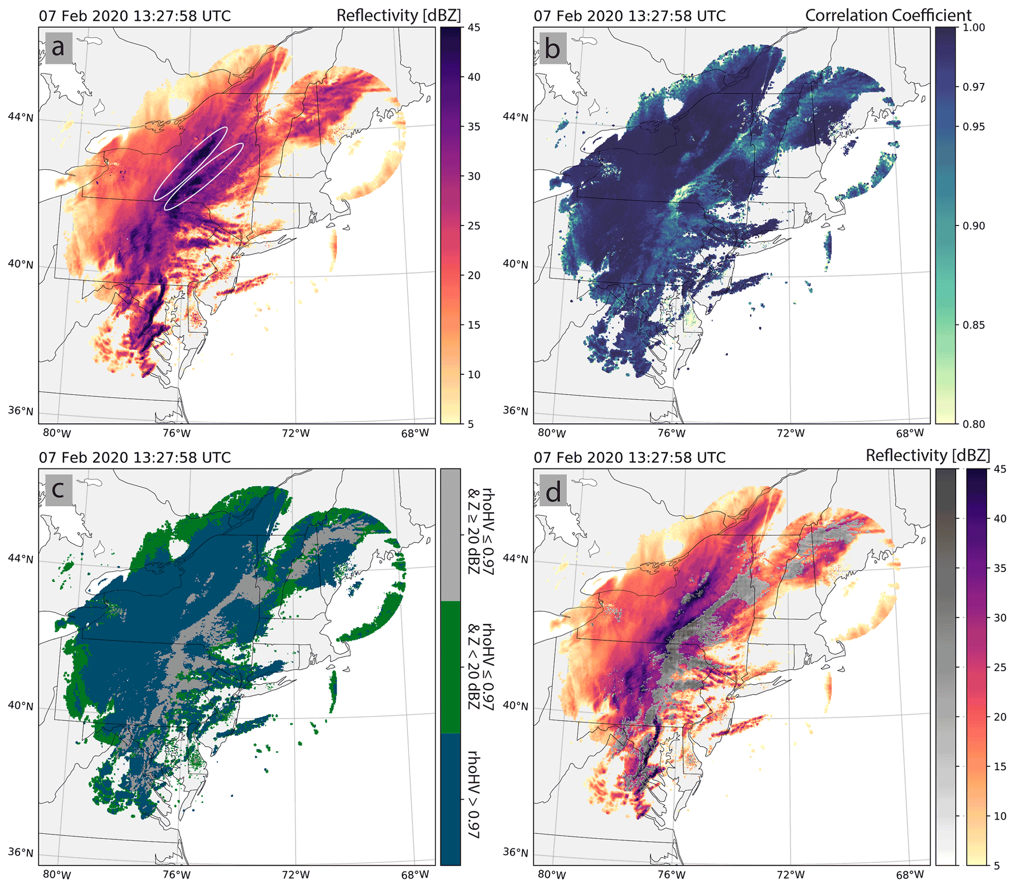
Figure 1 Image-muting processing components for a radar regional map from 7 February 2020 at 13:27:58 UTC. (a) Radar reflectivity (dBZ) field. (b) Correlation coefficient field. (c) Categories indicating regions that meet the following conditions: correlation coefficient >0.97 (dark blue), correlation coefficient ≤0.97 and reflectivity <20 dBZ (green), and correlation coefficient ≤0.97 and reflectivity ≥20 dBZ (gray). (d) Final image muted product combining color scale for reflectivities in snow and rain regions with gray scale to mute reflectivities in mixed precipitation regions. White ovals in the panel (a) indicate banded features discussed in the text. An animated version (Animation-Figure-1) of this figure is in the Video supplement.

3 Evaluation with independent data

Vertical cross-sections from airborne radar data provide an opportunity to evaluate the identification of melting regions in ground-based scanning radar data in fine detail. Figure 2 shows an image-muted regional map corresponding to a science flight during the NASA Investigation of Microphysics and Precipitation for Atlantic Coast-Threatening Snowstorms (IMPACTS) 2020 field project (McMurdie et al., 2022). Reflectivity from the nadir-pointing ER-2 X-band Doppler Radar (EXRAD; Heymsfield et al., 1996) along the flight track (green line) in Fig. 2a is shown in Fig. 2b. The gray region in the image- muted regional map indicates a quasi-linear region of mixed precipitation extending through eastern New York up to Vermont and New Hampshire (Fig. 2a) between areas of primarily snow (to the northwest in upstate New York) and primarily rain (to the southeast over southern New England). Eastward of 175 km along the flight transect in Fig. 2b, there is a clear melting layer signature in the NASA EXRAD data starting near the surface and rising to about 2 km above sea level (ASL) (represented by the enhanced region of higher reflectivity). The melting layer can also be observed with other variables from the same transect presented in Fig. 3. In particular, the linear depolarization ratio from the ER-2 cloud radar shows the structure of the melting layer very well (Fig. 3d). Under the melting layer, the values of downward pointing Doppler velocity $<-\mathrm{4}$ m s⁻¹ indicate the rain layer. The position of the transition between snow and rain in the vertical cross-section is consistent with the edge of the gray area in Fig. 2a. An animated version of Fig. 2 (Animation-Figure-2) shows the timing as the ER-2 aircraft transects through the image-muted portion of the regional map. As the airplane reaches around 175 km in the transect, one can see that the height of the NEXRAD radar beam used to create the regional map (black X in Fig. 2b) begins to intersect the melting layer.

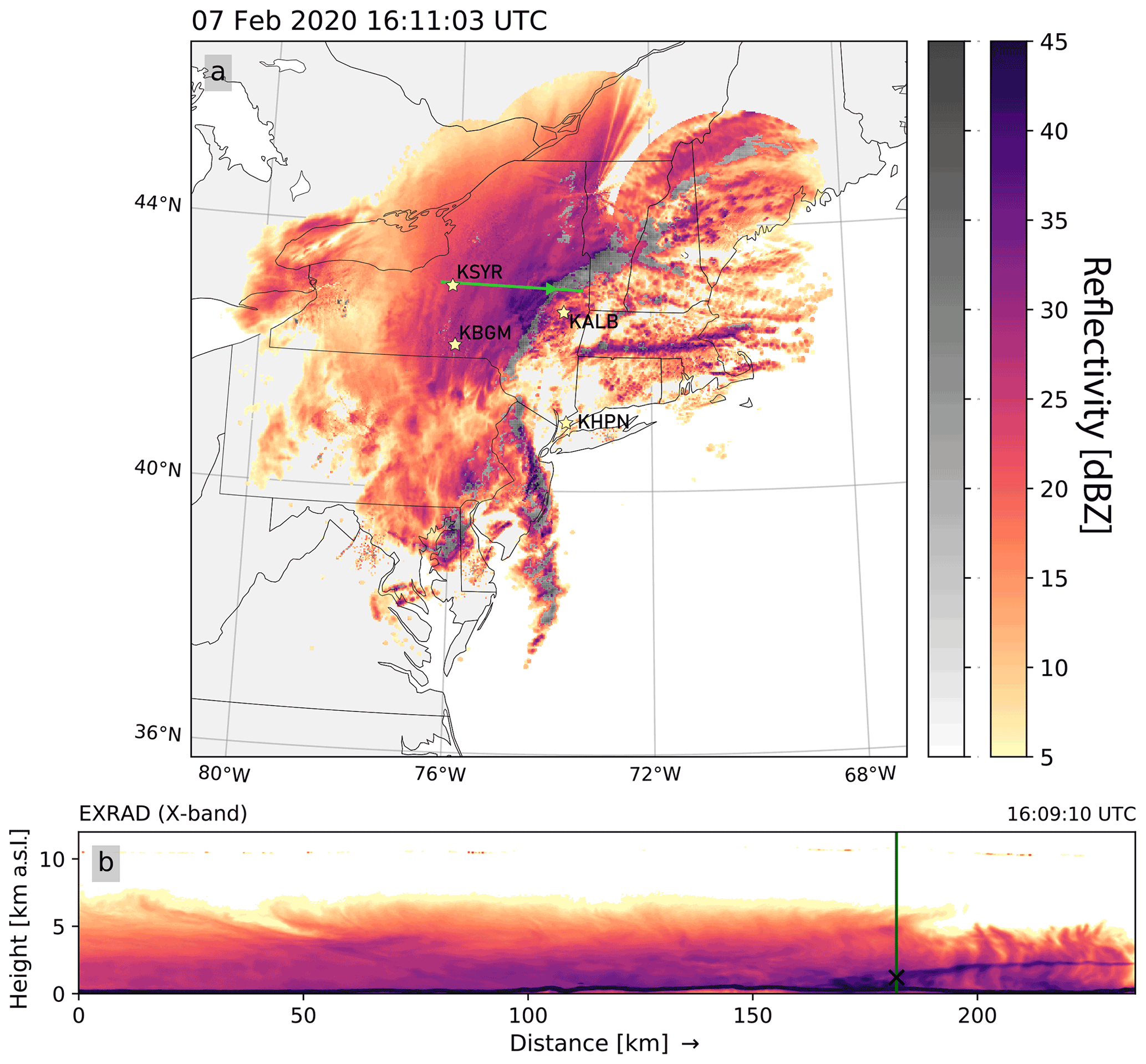
Figure 2 Comparison of image-muted regional map with detailed vertical cross-section from NASA ER-2 X-band Doppler radar during a NASA IMPACTS science mission on 7 February 2020. At 16:09:10 UTC, the aircraft is located at the transition between snow and melting precipitation in the radar regional map. (a) Image-muted reflectivity valid at 16:11:03 UTC with the ER-2 flight leg (green line), aircraft location corresponding to the time shown in the bottom panel is at the arrowhead along the leg. Locations of ASOS observations in Fig. 4 are annotated with stars and black labels. (b) Vertical cross-section of reflectivity from the NASA EXRAD radar with current aircraft location near the top of the vertical green line. Time on the right corresponds to the aircraft position. The black X indicates the height of the point in panel a that varies along the 0.5^∘ elevation angle scans used to construct the regional maps. An animated version of this figure (Animation-Figure-2) is in the Video supplement.

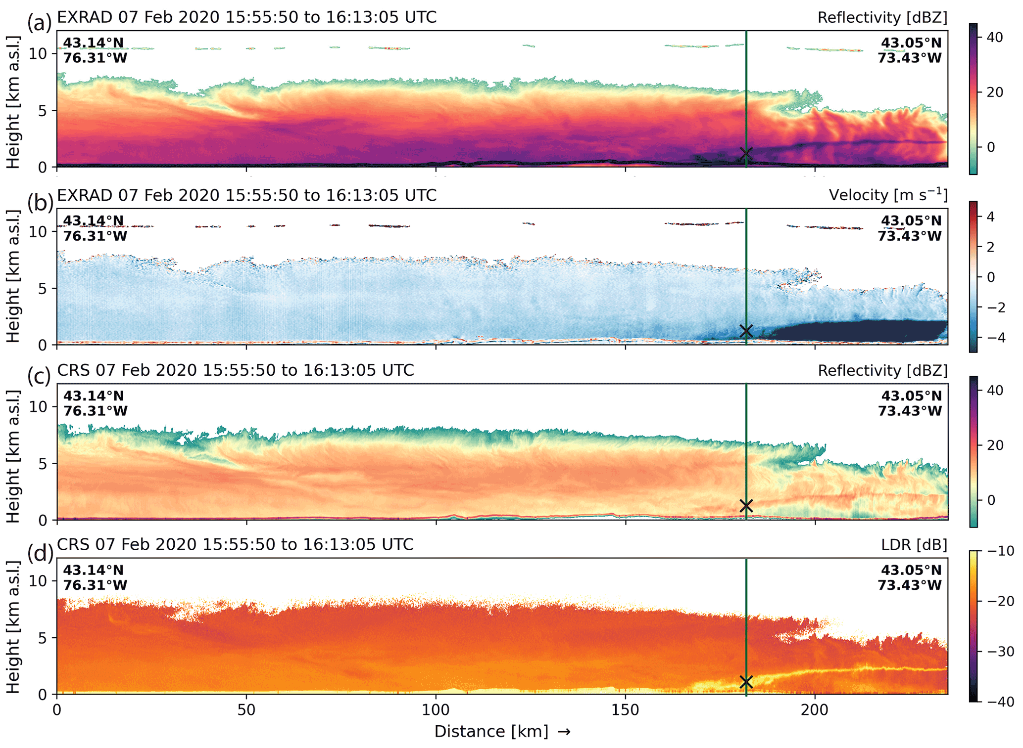
Figure 3 Vertical cross-sections of (a) reflectivity and (b) vertical velocity from the NASA ER-2 EXRAD radar and (c) reflectivity and (d) linear depolarization ratio (LDR) from the NASA ER-2 CRS radar coincident with the vertical cross-section in Fig. 2. Green line indicates current aircraft location and black X indicates the height of the point in Fig. 2a that varies along the 0.5^∘ elevation angle scans used to construct the regional maps.

Information to further evaluate the timing and location of the melting and mixed precipitation is available from time series of precipitation from surface sensors. Figure 4 shows hourly time series of precipitation types at several NWS Automated Surface Observing Systems (ASOS) weather stations (letters in Fig. 2a). The surface observations and timing of precipitation transitions align well with the evolution and movement of the storm (Figs. 2 and 3). For the hour of 16:00:00 UTC, Syracuse Hancock International Airport (KSYR) is reporting snow, Albany International Airport (KALB) is reporting rain, Greater Binghamton, NY (KBGM) is reporting snow, and Westchester County Airport (KHPN) is reporting rain. The ASOS time series for KBGM also indicates the hour when rain transitioned to mixed (11:00:00 UTC) and mixed transitioned to snow (15:00:00 UTC) (Fig. 4c). These surface data are consistent with the locations of the muted precipitation (see Animation-Figure-2).

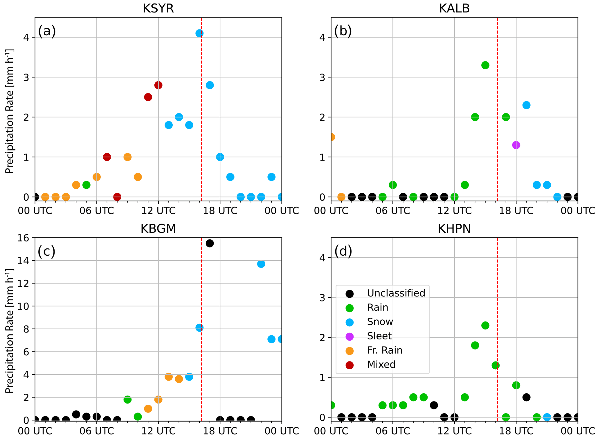
Figure 4 Hourly ASOS precipitation rate and type [mm h⁻¹] reports for 7 February 2020 from (a) KSYR, (b) KALB, (c) KBGM, and (d) KHPN. Colors indicate precipitation type as in the legend in panel (d). The dashed red line indicates 16:09:11 UTC, highlighted in Fig. 2. The y-axis range is larger in panel (c) than in the other panels.

4 Application to RHIs

Information on the 3D geometry of melting regions can be obtained by applying the image-muting technique to range-height indicator (RHI) scans constructed from a full volume scan from ground-based scanning radars. These examples illustrate the often complex layering within coastal winter storms, where portions of the warmer air masses (>0 ^∘C) slide over colder air masses (<0 ^∘C). Figure 5 is from the KOKX radar during a winter storm on 8 February 2013. The green line in the PPIs corresponds to the azimuth used to create the RHIs (Fig. 5a, b). Rather than a simple flat or tilted melting layer, this storm had a 3D “arc-like” mixed precipitation structure (Fig. 5c, d). The temperature field along the RHI from the ERA5 reanalysis data shows the associated vertical temperature structure and the 0 ^∘C isotherm (Fig. 5e; Hersbach et al., 2020). Below 2 km ASL, the temperature is mostly above freezing, which corresponds well with the top of the melting in the RHI panels (Fig. 5c, d, e). There appears to be an intrusion of colder air around 0.5 km ASL (0–30 km horizontal) that is likely contributing to the arc-like feature seen in the RHI panels (Fig. 5c, d, e). Animations of panels (a) through (d) of Fig. 5 show the complex horizontal pattern as the features evolve and move (see Animation-Figure-5). The structure of the melting layer in this example is also discussed in Griffin et al. (2014).

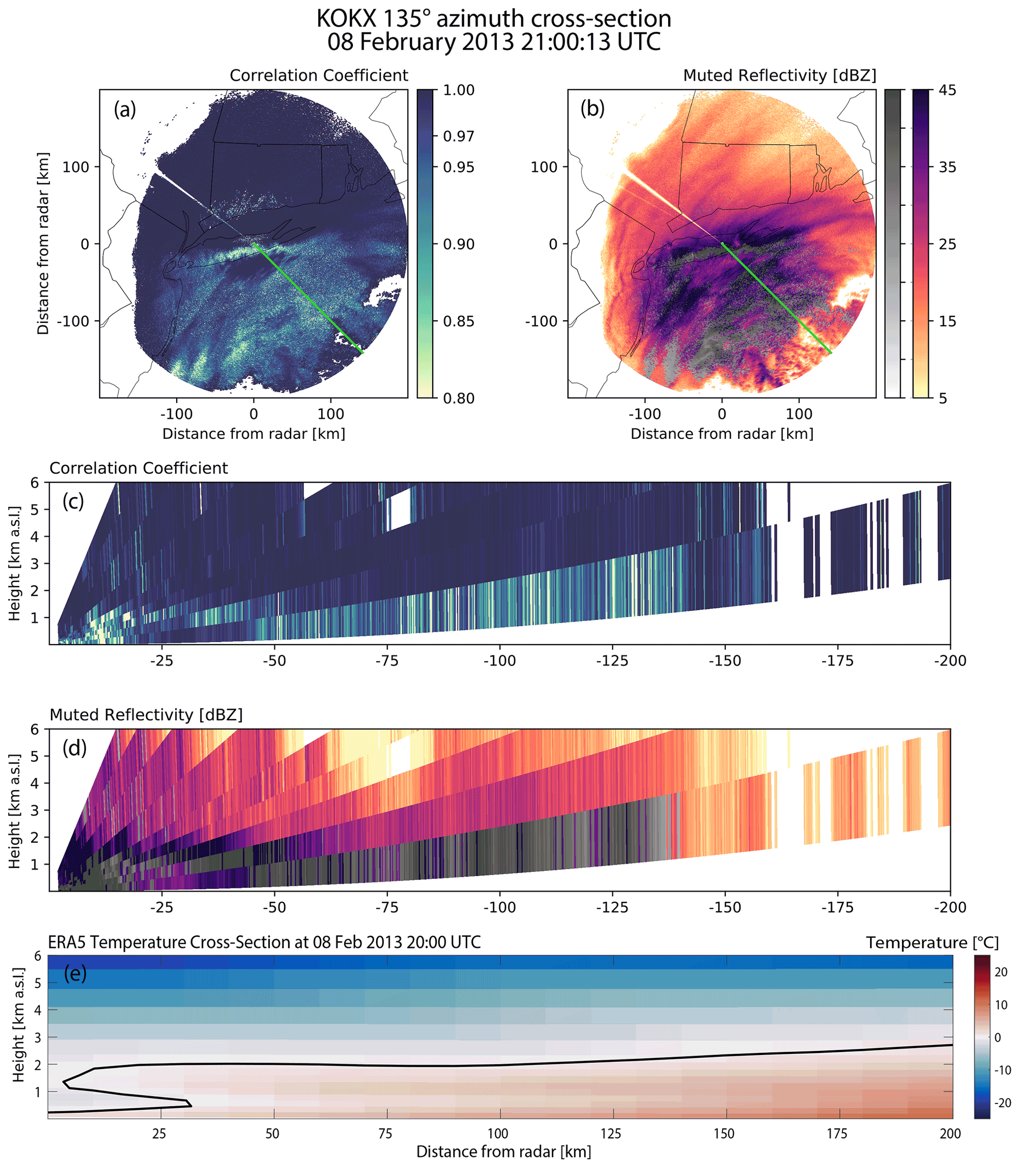
Figure 5 Comparison of image-muted regional map with reconstructed RHIs and reanalysis temperature vertical cross-section from the KOKX radar on 8 February 2013. (a) Correlation coefficient and (b) image-muted reflectivity (dBZ) 0.5^∘ elevation angle PPI plots for the KOKX radar valid 8 February 2013 21:00:13 UTC. Green line in panels (a) and (b) indicates the location of the reconstructed RHI cross-sections from (c) the correlation coefficient and (d) image-muted reflectivity. (e) ERA5 reanalysis temperature cross-section interpolated to the plane of the RHI. Black line in panel (e) indicates 0 ^∘C isotherm. An animated version of this figure (Animation-Figure-5) is in the Video supplement.

An example from the Philadelphia, PA (KDIX) radar during a winter storm on 1 December 2019 is presented in Fig. 6. This storm exhibited an interesting “collapsing” signature in the correlation coefficient and image-muted reflectivity PPI fields in northern New Jersey (Fig. 6a, b). The RHI panels intersect the feature and show a sharp drop in melting layer altitude around the 80 km range from the radar (Fig. 6c, d). The temperature field from the ERA5 reanalysis shows an elongated layer of above freezing temperatures around 2 km ASL and another area of above freezing temperatures below 1 km ASL between 0 and 50 km away from the radar (Fig. 6e). It is likely that the ERA5 data are too coarse to fully represent the complex temperature structure, as suggested by the radar RHIs. Animations of panels (a) through (d) of Fig. 6 show the initiation of this feature and how it evolves (see Animation-Figure-6).

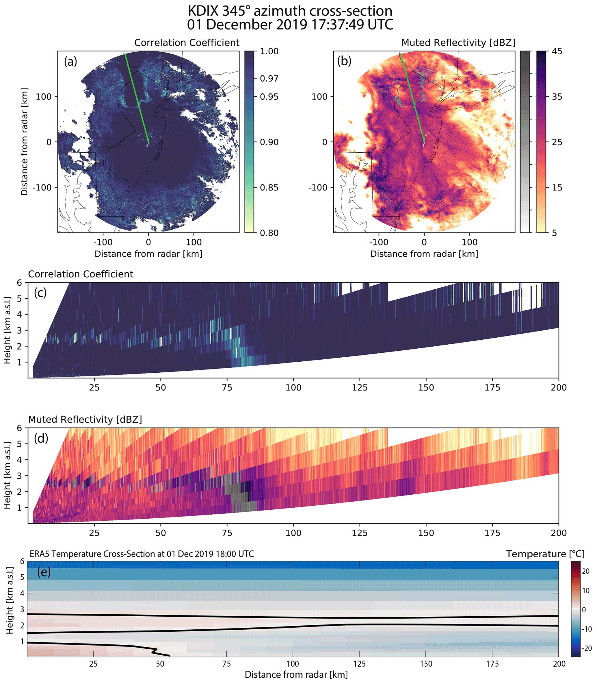
Figure 6 Comparison of image-muted regional map with reconstructed RHIs and reanalysis temperature vertical cross-section from the KDIX radar on 1 December 2019. (a) Correlation coefficient and (b) image- muted reflectivity (dBZ) 0.5^∘ elevation angle PPI plots for the KDIX radar valid 1 December 2019 17:37:49 UTC. Green line in panels (a) and (b) indicates the location of reconstructed RHI cross-sections from (c) the correlation coefficient and (d) image-muted reflectivity. (e) ERA5 reanalysis temperature cross-section interpolated to the plane of the RHI. Black line in panel (e) indicates 0 ^∘C isotherm. An animated version of this figure (Animation-Figure-6) is in the Video supplement.

Users should use caution interpreting features at longer ranges from the radar where ρ_HV suffers from quality issues related to a low SNR. For example, in Fig. 6, the speckled muting beyond 100 km range of the radar is likely the result of the superposition of an increase in correlation coefficient associated with a low SNR and a decrease associated with melting. Animation-Figure-6 illustrates that the concentric speckled region remains approximately stationary to the radar and hence can be visually distinguished from advecting reflectivity bands.

5 Summary

The proliferation of weather radar web interfaces and mobile apps has made operational radar data easily accessible to a wide range of users with varying levels of radar data interpretation expertise. People who are well versed in the subtle nuances of interpreting weather radar data represent only a subset of research meteorologists and an even smaller subset of the broader set of radar data users, which includes emergency managers, TV weathercasters, and airport operators.

Users of weather radar data associate areas of higher reflectivities with heavier precipitation. In winter storms, linear features of localized enhanced reflectivity are associated with heavy snow bands and contribute to snow accumulation forecast uncertainties (e.g., Novak et al., 2008; Ganetis et al., 2018). But regions of mixed precipitation can exhibit higher reflectivities, often without the higher precipitation rates or equivalent liquid water content. For winter storm analysis, it is important to distinguish between locally enhanced reflectivity associated with increases in ice mass and reflectivity from melting. Fortunately, mixed precipitation often has a low correlation coefficient (<0.97), which in combination with reflectivities ≥20 dBZ can be used to distinguish higher reflectivity regions that are and are not heavy snow (Giangrande et al., 2008).

Typically, radar reflectivity and hydrometeor identification are presented as separate products (Rauber and Nesbitt, 2018; Bringi and Chandrasekar, 2001; NOAA, 2017). When these products are separate, a user examining an evolving winter storm needs to simultaneously examine synced sequences of maps and mentally keep track of the moving positions of higher reflectivity features relative to the hydrometeor-type signatures.

We developed image muting, which reduces the visual prominence of the reflectivities within the mixed precipitation features in winter storms that can be misidentified as heavy snow. Reflectivities corresponding to the mixed precipitation features are de-emphasized using a gray scale and the regions with just snow and just rain are depicted in a corresponding full-color scale. We tuned the thresholds used for identification of mixed precipitation areas using a combination of detailed vertical cross-sections from research aircraft radar, reconstructed RHIs from ground-based scanning radars, and surface weather stations observed precipitation types. Users could apply this visualization technique using operational hydrometeor classification as an input and mute other specific regions depending on the application.

Enhanced reflectivity bands that are snow or contain mixed precipitation will generally move consistently with the advection of other reflectivity features rather than being fixed either concentrically or radially to the radar position. Hence, our image-muting method is best used as part of movie loop sequences rather than as individual images. Image-muted movie loops will help to reduce the error associated with misinterpreting radar reflectivity products during winter storms. Users examining an image-muted 2D map movie loop can more easily distinguish the locations of heavy snow and mixed precipitation than if they had to consult separate movie loops. Monitoring where transitions from rain to mixed precipitation and mixed precipitation to snow are present and where they are likely to move can aid in assessing expected impacts of winter weather.

The method of detecting melting regions is not perfect, in large part because such algorithms are limited by the input data quality. For US NEXRAD data, without improvements in the data quality of ρ_HV, detection of melting regions, particularly at more distant ranges will be more speckled than at closer ranges. If the SNR field is made available it can be used to filter out questionable ρ_HV values and improve the detection of melting regions. Users are advised to utilize movie loops to assess the time and spatial continuity when distinguishing band-like enhanced reflectivity features corresponding to heavy snow bands from those that include melting.

The image-muting visualization technique can be applied to a wide variety of applications. Any data display that suffers from potential misinterpretation could benefit from image-muting portions of the data to de-emphasize subregions in the plot.