the Creative Commons Attribution 4.0 License.
the Creative Commons Attribution 4.0 License.
 | 10 Oct 2022
An improved vertical correction method for the inter-comparison and inter-validation of integrated water vapour measurements
Pierre Bosser
Carl Mears
Integrated water vapour (IWV) measurements from similar or different techniques are often inter-compared for calibration and validation purposes. Results are usually assessed in terms of bias (difference of the means), standard deviation of the differences, and linear fit slope and offset (intercept) estimates. When the instruments are located at different elevations, a correction must be applied to account for the vertical displacement between the sites. Empirical formulations are traditionally used for this correction. In this paper we show that the widely used correction model based on a standard, exponential, profile for water vapour cannot properly correct the bias, slope, and offset parameters simultaneously. Correcting the bias with this model degrades the slope and offset estimates and vice versa. This paper proposes an improved correction method that overcomes these limitations. It implements a multiple linear regression method where the slope and offset parameters are provided from a radiosonde climatology. It is able to predict monthly mean IWVs with a bias smaller than 0.1 kg m−2 and a root-mean-square error smaller than 0.5 kg m−2 for height differences up to 500 m. The method is applied to the inter-comparison of GPS IWV data in a tropical mountainous area and to the inter-validation of GPS and satellite microwave radiometer data. This paper also emphasizes the need for using a slope and offset regression method that accounts for errors in both variables and for correctly specifying these errors.
- Article
(6134 KB) - Full-text XML
- BibTeX
- EndNote


Water vapour plays a key role in many meteorological processes and in the hydrological cycle of the Earth's atmosphere. Because it is extremely heterogeneous and variable, many operational and research observing techniques have been developed over the years to sense its horizontal, vertical, and temporal variability. Among the various high-performing techniques, one may cite in situ measurements with radiosonde balloons and remote sensing techniques exploiting different domains of the electromagnetic spectrum, namely Fourier transform infrared radiometers (FTIR); near-infrared, visible, and ultraviolet radiometers and spectrometers; microwave radiometers (MWRs); and microwave measurements from global navigation satellite systems (GNSS). Integrated water vapour (IWV) measurements from ground-based and space-based platforms are often compared to assess each other's accuracy, e.g. detect biases and/or long-term drifts (Bokoye et al., 2003, 2007; Morland et al., 2006a, b, 2009; Bock et al., 2007, 2014, 2021; Sussmann et al., 2009; Bedka et al., 2010; Palm et al., 2010; Schneider et al., 2010; Vogelmann et al., 2011; Buehler et al., 2012; Cimini et al., 2012; Van Malderen et al., 2014; Courcoux and Schröder, 2015; Schröder et al., 2016), as well as for inter-calibration purposes, e.g. adjusting biases from instruments on successive space-based platforms (Du et al., 2015; Mears et al., 2015, 2018; Wentz, 2015; Bennartz et al., 2017; Ho et al., 2018; Schröder et al., 2019). In this context, it is frequent that IWV measurements from sites at different elevations need to be compared (e.g. Bock et al., 2005; Morland et al., 2006a; Buehler et al., 2012; Van Malderen et al., 2014). Because the water vapour concentration in the atmosphere decreases by several orders of magnitude between the surface and the upper troposphere, a vertical correction is required to conform the measurements from sites at different altitudes or between point observations and aerial averages, such as those derived from atmospheric models (Bock et al., 2005, 2007, 2014; Morland et al., 2006b; Buehler et al., 2012). There is a similar problem for the vertical adjustment of tropospheric wet delays (Dousa and Elias, 2014). While many studies have recognized that a height difference results in a systematic difference (bias) in the IWV measurements, few have applied a correction, and even fewer have recognized that the height difference also impacts the linear fit slope and offset estimates. To our knowledge, only Bock et al. (2005), Morland et al. (2006a, b), Buehler et al. (2012), and Van Malderen et al. (2014) addressed these points. Van Malderen et al. (2014) experienced that applying a scaling factor for correcting the bias degrades the slope estimate. Buehler et al. (2012) analysed the impact of height difference on the slope estimate using radiosonde data and proposed using this estimate to correct the IWV data. We will follow a similar methodology in this paper with an improved model. Among the correction models that have been proposed by various authors, two approaches have been traditionally used. The first and most widely used approach is based on a proportional correction term that has its roots in the assumed exponential decrease of water vapour concentration with height. This model is described in Appendix A. It makes use of the assumption of a constant vertical decay rate of water vapour, γ. At least three studies have applied this correction model, and they proposed very similar experimental values for γ; namely, Bock et al. (2005) proposed m−1 for the Alps, Morland et al. (2006a) proposed m−1 also for the Alps, and Buehler et al. (2012) proposed m−1 for Antarctica. These models have been claimed by their authors to be valid for height differences up to 500 m. The second approach, proposed by Mears et al. (2015), is based on the observed sea surface temperature and a constant relative humidity of 80 %. They applied this model for the inter-comparison of satellite-based MWR measurements with ground-based global positioning system (GPS) stations with elevations that are usually less than 100 m and one exceptional case above 500 m for which it still worked well. Both approaches have been shown to provide acceptable reductions in the differential IWV biases.
In this paper, we show that the exponential correction cannot simultaneously achieve a proper correction for the bias, the slope, and offset parameters. To overcome this limitation, we propose an improved vertical correction method based on multi-linear regression from a radiosonde climatology. Another aspect discussed in this paper is the impact of errors in both variables on the slope and offset estimates. Contrary to trend estimation, where a physical variable is regressed in time (a quantity known with negligible error), the linear regression between two measurements that are both subject to errors requires a more elaborate estimation method. Indeed, it has been shown that in this situation, the ordinary least-squares (OLS) regression leads to biased estimates of the slope and offset (Draper and Smith, 1998). This problem has clearly been overlooked in the aforementioned IWV inter-comparison literature. This may be at least one reason for the variety of slope results found in these studies (with the slope being either bigger or smaller than 1). Comparing slope and offset results from different studies, as was done in, e.g. Buehler et al. (2012), may therefore be hazardous as different and sometimes incorrect regression methods have been used. Only a few of these studies stated explicitly that they used a regression method accounting for errors in both variables (e.g. Buehler et al., 2012; Bock et al., 2014, 2021). Using such a method also poses the problem of correctly specifying the uncertainties in both variables. Lack of such information for some of their data sets led Buehler et al. (2012) to apply OLS regression and to state that constant error estimates do not affect the regression results, which is wrong (see Appendix C). Instead, Bock et al. (2014, 2021) used approximate error estimates, e.g. 5 % or 10 % for radiosonde or satellite data, rather than assuming no errors in the x variable. In this paper, we use the three-way error analysis of O'Carroll et al. (2008) to specify the uncertainties of our data sets and the regression method of York et al. (2004), which accounts for errors in both variables.
Section 2 of this paper reviews the impact of a height difference on the bias, slope, and offset estimates in the case of an idealized exponentially decaying water vapour density profile and in the case of a real atmosphere observed by radiosondes. The similarities and differences implied by two types of profiles are highlighted. Section 3 proposes an improved vertical correction method based on a multiple linear regression approach, instead of using one single γ parameter as was done in past studies. The method builds on a climatology derived from radiosonde data. In Sect. 4 we discuss two application examples where IWV measurements from a network of GPS stations in a tropical mountainous area are to be inter-compared and used for the inter-validation with co-located satellite MWR measurements. Both applications make use of the new method and the derived radiosonde climatology. Section 5 discusses further applicability of the method and concludes.
2.1 Idealized case of an exponentially decaying water vapour density profile
Before analysing the results from real data, it is instructive to consider the idealized case of a water vapour density profile decaying exponentially with height (Eq. A1). This model has often been used to describe the state of the mean atmosphere (e.g. ITU, 2017) and is related to the notion of water vapour scale height (see Appendix A).
Let us consider the situation of two instruments, A and B, located at sites with different heights, hA and hB, which are observing IWV in an idealized atmosphere described by Eq. (A1). In the absence of any instrumental bias and noise, the IWV observations are related by
where γ>0 is the vertical decay rate of water vapour, which is related to the water vapour scale height by the relation . If hB>hA, we have IWVB<IWVA, meaning that the IWV content at higher altitudes is lower than the IWV content at lower altitudes. If the observations from station A and B are directly compared without any correction, we will observe a negative bias, , a slope smaller than 1, α<1, and a null offset, β=0, where the slope and offset are estimated by a linear regression using the model , with y=IWVB and x=IWVA (see Appendix B).
To be a bit more general, we can assume that the observations contain some amount of random noise and consider that we have n pairs of observations, (xi,yi), i=1…n, from which the bias, slope, and offset parameters are estimated. The bias is written as follows:
where μx and μy denote the sample means of the two data series. From Eq. (1), and introducing , with , the bias can be expressed as follows:
The first right-hand side (rhs) will be used later to describe the more general atmospheres. The second rhs is valid only in the case of the exponentially decaying water vapour profile. It expresses that the bias is proportional to the mean IWV content at the reference site, μx, and that it is negative given that γ>0 and Δh>0. The last rhs is the approximate relation valid for a thin layer (typically, m, see Appendix A) and expresses that, to the first order, the bias is proportional to μx, γ, and Δh. This last expression has been used in past studies (e.g. Bock et al., 2005; Buehler et al., 2012) to estimate the vertical moisture decay rate, , and to correct IWV observations for the height difference between sites. The slope and offset parameters estimated from the linear regression establish a second relation between μx and μy given by Eq. (B3), which can be rewritten in the case of the exponential water vapour profile as . Since this relation must be valid for any μx, it comes out that
The second rhs of Eq. (4a) expresses that α<1, given that Δh>0, and the third rhs expresses that, to the first order, α decays linearly with the height difference, with a rate equal to γ.
Figure 1 illustrates the main characteristics of the bias and slope variations with height in the case of the idealized exponential water vapour profile, along with the asymptotic limits and the thin-layer linear approximations. It is important to note that both the bias ( is increasing when is increasing) and the slope ( is increasing when is increasing) change when the depth of the atmospheric layer Δh changes.
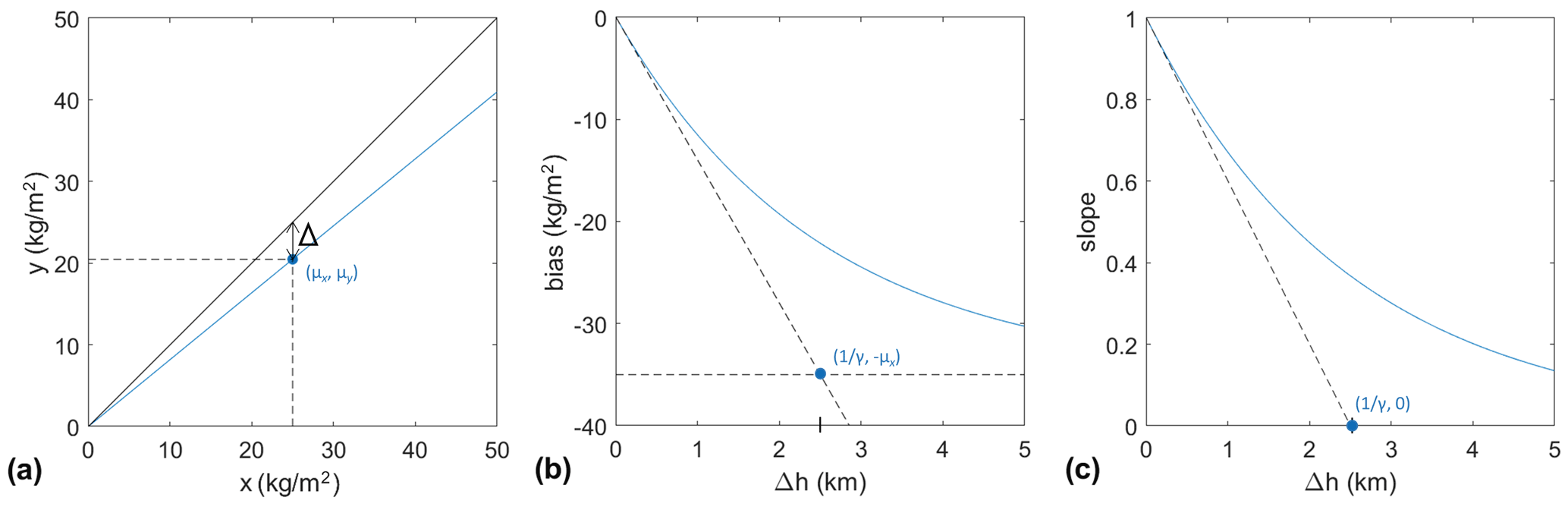
Figure 1Illustration of the variation in IWV as a function of height in the case of an idealized moisture profile with exponential vertical decay with a rate m−1 (scale height km): (a) as a function of x for a fixed Δh>0; (b) bias, , as a function of Δh (Eq. 3); and (c) slope, α, as a function of Δh (Eqs. 4a and 4b). The slanted dashed lines in panels (b) and (c) represent the thin layer approximations (rightmost sides of Eqs. 3, 4a and 4b, respectively).
Equations (3) and (4a) also recall that both the bias and slope parameters depend on the atmospheric profile through the γ parameter, which may be of relatively localized in nature and may thus change from one region to another and vary with time, e.g. seasonally. Moreover, in real atmospheres, the vertical distribution of water vapour is expected to be more complex than can be represented by an exponential model with a constant vertical decay rate.
2.2 Real case from radiosonde observations
Figure 2 illustrates the monthly mean water vapour profiles observed by a tropical radiosonde station (Le Raizet, Guadeloupe, France, WMO code 78897) over the year 2020. It can be seen that the water vapour is decaying approximately exponentially, although the vertical decay rate is not strictly constant as a function of height and time. This model is nevertheless reasonable in the lower troposphere, i.e. from the surface up to a height of 2 km (Fig. 2b). In this altitude range, we expect Eq. (1) to be a good approximation of the vertical variation in IWV. Figure 2c illustrates the link between x=IWV(hs) and , where and , and where ρv(h) is the observed radiosonde water vapour profile, hs is the station height, and Δh varies between 200 and 1000 m in steps of 200 m. For each layer, Δh, the points (x,y) align roughly on a straight line. For Δh=200 m, the line is closest to the 1:1 line (shown in grey) and the scatter around the best-fit line is the smallest (RMSE=0.224 kg m−2), while for Δh=1000 m, the line is farthest from the 1:1 line and the scatter around the best-fit line is the largest (RMSE=0.976 kg m−2). It is interesting to note that for a given layer, Δh, the points remain close to the straight line throughout the year, despite the quite large seasonal excursion in IWV shown by the different colours in the figure. The data points for March are shown as light blue dots, and the data points for September are shown as orange dots. These two months show the smallest and largest mean IWV values, μx, of 33 and 51 kg m−2, respectively.
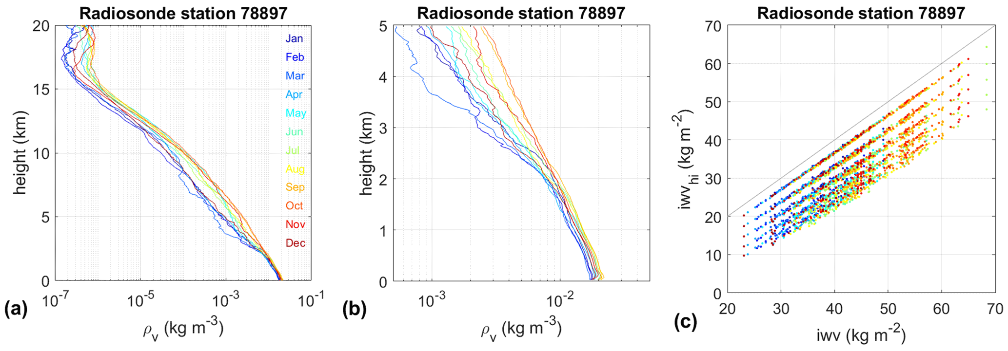
Figure 2Real water vapour profiles observed by radiosonde station 78897 (Le Raizet, Guadeloupe, France): (a) monthly mean profiles for the year 2020. Panel (b) is similar to (a) for altitudes below 5 km. (c) IWV scatter plot, with upper-level IWV plotted on the y axis and total column IWV on the x axis for five different height differences: Δh=200, 400, 600, 800, and 1000 m. The radiosonde data include 00:00 and 12:00 UTC soundings. The colour code indicated in panel (a) is valid for all plots.
Figure 3 shows the variations of the bias, offset, and slope parameters fitted from these data, as a function of Δh. The bias (Fig. 3a) and the fractional bias () (Fig. 3d) follow the exponential decay predicted by the second rhs of Eq. (3) reasonably well, but the lines do not actually align perfectly from 1 month to another, because of the small seasonal variations in the humidity profile. The monthly variation is even more visible in the slope and offset plots (Fig. 3b and c). However, each monthly curve for the slope may be reasonably well modelled by an exponentially decaying function described by the second rhs of Eq. (4a). Regarding the offset, the purely exponentially decaying water vapour profile predicts β=0, which is clearly not verified in the real atmosphere. However, all three parameters together follow the relationship described in Appendix B, i.e. α<1 and Δ<0 imply that β>Δ. Figure 3c shows that β actually follows the variation in Δ closely as a function of Δh, while verifying β>Δ. Figure 3b and c also show that the slope and offset estimates are correlated to each other, meaning that higher slopes are associated with smaller offsets (Walpole et al., 2012). Figure 3e and f show the standard errors of the α and β parameters estimated by OLS given by Eqs. (C4), (C5a), and (C5b). They are increasing with Δh as expected from the increased scatter of the post-fit residuals (Fig. 2c). In Sect. 3 we will establish a model describing the behaviour of α and β as a function of Δh that will be used to correct the observations x made at a height hA to conform to the observations y made at height .
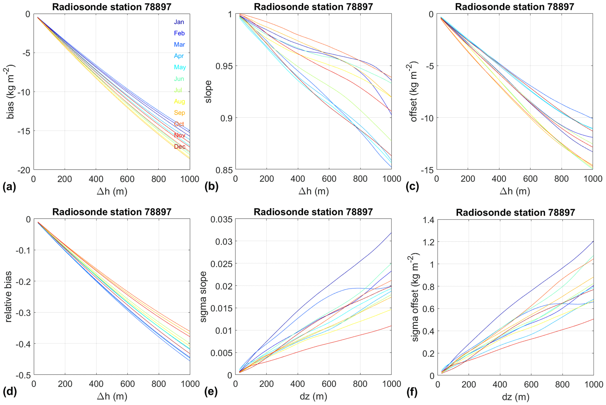
Figure 3Monthly mean estimates computed from the radiosonde observations shown in Fig. 2c for Δh=25 to 1000 m in steps of 25 m: (a, d) bias, Δ, and relative bias, ; (b, c) slope and offset parameters fitted from Eq. (B2) by ordinary least squares; (e, f) standard errors of the slope and offset parameters.
In the previous section we have seen that the bias, Δ, and the slope, α, are dependent on the depth, Δh, of the layer between the two considered IWV observations. In particular, and are both increasing when is increasing, both in the real atmosphere and in the idealized, exponentially decaying, atmosphere. Whereas the offset is β=0 in the idealized atmosphere, it is generally β≠0 in the real atmosphere. The main difference between the idealized and real atmospheres is that the vertical moisture decay rate γ is dependent on the height (and time) in the latter, whereas it is by definition constant in the former (although a time variation could also be modelled in the idealized atmosphere). We must thus derive a correction formula based on a more complex model than just a constant γ. Moreover, a pure rescaling correction, , as discussed in Appendix B, does not allow us to simultaneously correct the bias and slope and does not change the offset. Instead, we propose using a linear correction model such as expressed by Eqs. (B8) and (B9). Therefore, we need good estimates for both α and β, which are generally not known at the location and time of interest but may be derived from a climatology. Hereafter, we propose using high-resolution radiosonde observations to derive such a climatology.
The proposed approach is to model the slope and offset with two independent functions of Δh:
which are represented by polynomials
Note that the polynomials have no intercepts in order to satisfy the constraints A(0)=0 and B(0)=0. Figure 3b and c suggest that the order of the polynomials does not need to be very high. For example, coefficient a1 can be identified with the vertical moisture decay rate, γ, in analogy with Eq. (4a). The higher-order terms help to model the deviations from linearity observed in Fig. 3b and c.
The estimates of the polynomial coefficients for each of the two models are derived by a linear regression method, according to the generic linear model equation: z=Xθ, where z is the vector of dependent variables, X the design matrix, and θ the vector of parameters (Walpole et al., 2012). The elements, zk, of vector z correspond either to the observed slope values, −log (αk), or to the offset values, βk, for the different layers, Δhk, k=1…m. The elements of the design matrix are Xik=(Δhk)i, and the parameters are θi=ai, with i=1…p, in the case of the slope model and θi=bi, with i=1…q, in the case of the offset model. Note that here we estimate the slope and offset coefficients independently of each other. Another approach might be to consider both variables simultaneously in a multivariate linear regression (Christensen, 2001), which is possible here since both variables are described by similar functional models, i.e. Eqs. (6a) and (6b). A few tests of this approach revealed that both the estimates and their standard errors were identical to the monovariate solutions. So we decided to stay with the monovariate linear regression approach, which is simpler to implement and faster to run.
The quality of the fitted models depends on the number of observations, m, and the choice of the polynomial orders, p and q. Indeed, larger layers would require us to include higher-order terms to adequately fit the deviations from linearity. The number of observations depends on the vertical sampling of the radiosonde profiles. Since we are using high-resolution radiosonde data, we can set a regular vertical sampling of Δh=25 m, i.e. . Considering two different maximal thicknesses of Δhm=500 and Δhm=1000 m, this leads to m=20 and m=40, respectively.
The order of the polynomials can be either fixed to predetermined values or determined automatically by a stepwise linear regression method (Hocking, 1976). The stepwise regression selects the best model by adding and removing terms to and from the model. The selection can be based on the p value of the F statistic associated with the change in the sum of squared errors (SSE) that results from adding or removing a term. Other types of criteria, such as the Akaike information criterion (AIC), the Bayesian information criterion (BIC), or the adjusted coefficient of determination , can be used as well (Draper and Smith, 1998). A few trials with different values for p (resp. q) revealed that all the aforementioned criteria (SSE, AIC, BIC, and ) lead to very consistent results and that the quality of the model is generally improved when p (resp. q) is increased. However, we also noticed that when p>5 (resp. q>5), the regression failed due to poor conditioning of the normal matrix, XTX. We consequently limited the regression to maximum orders p=5 (resp. q=5). The SSE criterion was used with the following limits for the p values: when pval<0.05, the term is added during the forward step, while when pval>0.10, the term is removed during the backward step. This method is, e.g. implemented in the stepwiselm function available in MATLAB (2017).
Another aspect of the implementation of the linear regression method is whether we consider the data as homoscedastic (the observations have constant variance) or heteroscedastic (the observations have different variance). Figure 3e and f suggest that a heteroscedastic model is plausible: the standard errors, σk,α and σk,β, of the “observations”, αk and βk, are generally increasing with k. Heteroscedasticity can be simply accounted for by specifying a diagonal weight matrix, W, where the diagonal elements are for the slope and for the offset, which are computed here from the standard errors, i.e. and . Note that the relative standard error is used in the case of the slope because we use log (α) and not α in the regression.
We conducted a large number of trials for different values of the model parameters, i.e. p=1…5, q=1…5, m=20 and m=40 (maximum layer depths of 500 and 1000 m), and weighted or un-weighted regression, and different data sets, i.e. monthly or yearly input data (i.e. α and β fitted month by month or from a full year of radiosonde profiles). We also compared the regression results from different radiosonde stations to assess the robustness of the method as well as the spatial variability of the fitted parameters. The results from the different trials were inter-compared on the basis of two quality criteria: the standard error of the regression, also called the root-mean-squared error (RMSE), and the standard error (SE) of the estimates (Draper and Smith, 1998). The RMSE quantifies the dispersion of the observed values, zk, around the predicted values, , adjusted for the degrees of freedom:
where is the prediction error and m−p is the degrees of freedom in the case of the slope (m−q in the case of the offset). The SE of the estimates is obtained from the variance–covariance matrix Q:
where σe is the standard deviation of the errors in the “observations”, an estimate of which is given by , and Q depends only on the regressors, Xi, and the weights, Wkk. In the case of the OLS, , while in the case of the weighted least-squares (WLS), . It is straightforward to show that in the case of OLS, a simple polynomial model such as expressed by Eq. (6a) and limited to the order p=1, leads to for large m. This result indicates that the SE of the parameters varies as . We may thus expect some benefit from performing the regression over more elevated layers, e.g. with m=40 compared to m=20, although the final SE also depends on the standard error of the regression, se, which is expected to be increasing when more elevated layers are included.
The results obtained from the trials are summarized below.
-
The RMSE is decreased when the order of the model (p or q) is increased. This result is expected as a higher-order model better fits the real data.
-
The RMSE is increased with WLS compared to OLS. This is a statistical property of OLS compared to WLS, i.e. OLS generally better fits the original data than WLS (Draper and Smith, 1998).
-
The SE of the estimates is increased when the order of the model is increased. This result is expected from the fact that more parameters are estimated with the same number of observations.
-
The SE of the estimates is decreased with WLS compared to OLS. This result is expected because OLS is no longer the best linear unbiased estimator when the errors in the data are not equal (Draper and Smith, 1998).
-
Both the RMSE and the SE are increased when more elevated layers (up to 1000 m compared to 500 m) are considered, despite the increase in the number of observations (m=40 compared to m=20).
The above results were found to be valid for both variables ( and zk=βk), when both time samplings (monthly and yearly) and the different stations are considered. They suggest preferably using high-order polynomials, WLS estimation, and a vertical extent of the regression adapted to the application, i.e. verifying the condition that the fitted model is not used beyond the fitting range. The fine tuning of the regression parameters can be further made by checking the errors in the bias, slope, and offset parameters after correction (see Figs. 5 and 6, discussed below). Apart from the setting of the regression model, an additional important point is to choose a proper time and space sampling.
Figure 4 shows the estimates for parameters a1 and b1 to illustrate the variability in time and space at three stations located in the Caribbean region (78526 is located 531 km to the north-west of 78897 on Puerto Rico, and 78954 is located 417 km to the south of 78897 on Barbados). The temporal variations at each of the three sites are significant (compared to the error bars) but correlated between the sites. These results indicate (i) that it may be preferable to use monthly regression coefficients rather than yearly and (ii) that the radiosonde climatology derived from one site may be applied to distant sites to some extent (e.g. a few hundreds of kilometres apart). We investigated the first point by analysing the IWV error after correction for monthly and yearly coefficients.
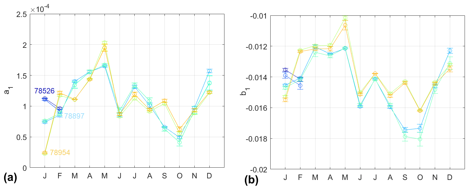
Figure 4Monthly estimates of the polynomial coefficients for the slope (a) and the offset (b) according to Eqs. (6a) and (6b), respectively, limited to order 1. The different curves show results for three different radiosonde stations (labelled by their WMO codes: 78897, 78954, and 78526) and two regression methods (OLS and WLS). The OLS and WLS results are almost superposed and are not labelled. Note that for station 78526 only 2 months of observations (January and February) were available in 2020. The error bars indicate the 95 % confidence interval for each estimated parameter.
Figure 5 shows the results when the coefficients are fitted by WLS, with , and a vertical range is limited to 500 m. Larger dispersion is clearly observed with the yearly model, with significant seasonal variation and an amplitude increasing with Δh. To quantify the impact of the second point, we used the model fitted for station 78954 to correct the data for station 78897. The resulting bias increased to 0.6 kg m−2.

Figure 5IWV correction error, , with (a) monthly coefficients and (b) yearly coefficients, as a function of time and height difference, Δh=25…500 m. Both models used polynomials of order 5 and weighted least-squares estimation. The time is colour coded in panel (a), while the height difference is colour coded in panel (b). The dots aligned in filaments correspond to a given time and varying Δh in both plots.
Finally, Fig. 6 shows the corresponding errors in the bias, slope, and offset parameters after correction for the model with monthly coefficients. The monthly mean bias remains negligible, kg m−2, and independent of the height difference, which demonstrates that the regression model is well parameterized. The standard deviation is increasing with the height difference up to 0.5 kg m−2 when Δh=500 m (this quantifies the dispersion observed in Fig. 5a). The slope and offset after correction are significantly improved compared to Fig. 3 and get very close to the ultimate objective (αc=1 and βc=0). We note that a smaller order of the polynomials could be chosen with the vertical range of 500 m, e.g. order 3 still achieves kg m−2, , and kg m−2. When the vertical range is raised to 1000 m, order 4 or 5 are recommended to achieve the same level of accuracy in Δc, but αc and βc are slightly degraded.
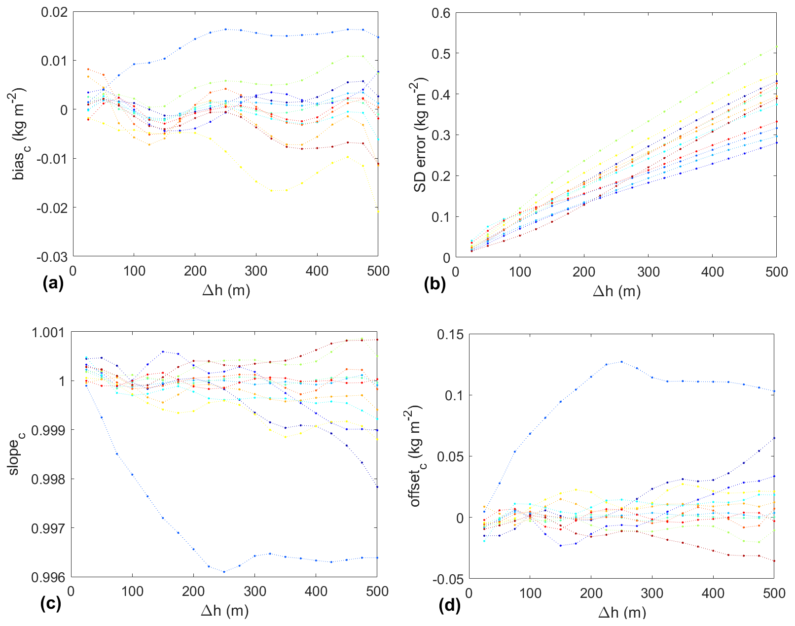
Figure 6Monthly mean bias (a) and standard deviation of the IWV correction error (b) with the monthly coefficients up to order 5 and WLS. Slope (c) and offset (d) parameters, αc and βc, respectively, of the best linear fit after correction, , as a function of time and height difference. The colour code for time is the same as in Fig. 2.
In conclusion, the proposed correction method is able to reduce almost perfectly the impact of the height difference on the IWV observations and achieve Δc≈0, αc≈1, and βc≈0, when a proper regression model is used. The correction model is expressed by Eqs. (B8) and (B9), where fc and gc are derived from the predicted values for and given by Eqs. (5) and (6). The estimates of the correction model are as follows:
4.1 GPS vs. GPS inter-comparison
Here we will consider the case of the permanent GPS network in Guadeloupe analysed by Bock et al. (2021) in the framework of EUREC4A, for the period from 1 January to 29 February 2020. It is composed of 15 stations located on four islands, in a region bounded by 15.75–16.75∘ N and 62–61∘ W. The station elevations range from 1 to 418 m (see Table 1). The ultimate goal of this inter-comparison is to determine the consistency of the IWV measurements from these GPS stations and to check for biases and non-linearities. Therefore, the IWV data need to be corrected for the height differences. Here we will consider both the simple scaling factor model, based on Eq. (A5), and the new model based on Eqs. (9a) and (9b). These correction models will be referred to as v1 and v2 in the following, and the uncorrected data will be denoted v0. The model coefficient in v1 is taken to m−1 consistent with Bock et al. (2007) for the tropics. In v2, we will use the coefficients determined from the radiosonde climatology derived in the previous section from the radiosonde station 78897, which is located on Guadeloupe, close to the GPS station ABMF. The bias, slope, and offset parameters derived from the inter-comparisons for the different data versions will be denoted Δv, αv, and βv, with , respectively.
Table 1Height above sea level and number of IWV estimates (N) for 15 GNSS stations over the Guadeloupe archipelago (15.75–16.75∘ N, 62–61∘ W) for the period from 1 January to 29 February 2020 (Bock et al., 2021).
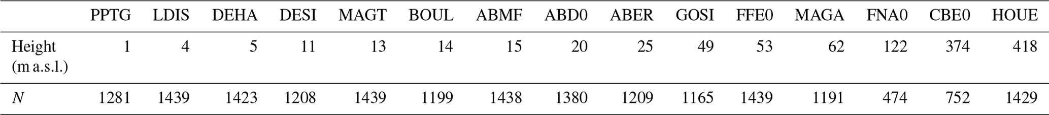
Figure 7 shows the results of the inter-comparison of two stations at very different elevations (ABMF: hA=15 m; HOUE: hB=418 m). It is seen that the initial bias of kg m−2 is quite large but consistent with the values predicted from the radiosonde data (Fig. 3) for such a large height difference. Both correction models significantly reduce the bias, although v1 has some residual bias, kg m−2, whereas v2 achieves kg m−2, i.e. almost perfect correction. Figure 7 also compares the slope and offset results estimated by two different regression methods: Fig. 7a–c used the OLS method, i.e. assuming no errors in the x variable, and Fig. 7d–f used the York et al. (2004) method. With the latter method, the formal errors provided by the GPS data-processing software were used as “observation errors”, after a rescaling by factor of 5 to be consistent with the traditionally assumed uncertainty of 1.5 kg m−2 for GPS IWV data (Bock et al., 2021). The initial slope and offset amount to α0=0.92 and kg m−2 with the OLS estimator and α0=0.97 and kg m−2 with the York estimator. The latter values are more in line with the values found from the radiosonde data (Fig. 3) and predict a higher slope. It is well known that the OLS slope estimator is biased low (towards zero) when the x variable contains random errors (Edland, 1996). This feature is clearly observed with all three data versions shown in Fig. 7. The results also verify the relationship between bias, slope, and offset sketched in Fig. B1, whatever the estimator. After correction with model v1, the slope becomes α1=1.08 with the OLS estimator and 1.15 with the York estimator, while correction with model v2 achieves α2=0.95 with the OLS estimator and 1.01 with the York estimator. Both estimators find that model v1 slightly overcorrects the data (α1>1). On the other hand, v2 performs much better and achieves almost a perfect slope (α1≈1) with the York estimator. Regarding the offset, we see that the value is unchanged with model v1, as predicted from Eq. (B7), whereas model v2 achieves nearly perfect correction (β2≈0). These results are highly consistent with those found in Sect. 3 from the radiosonde data. Regarding the initial question, we can state the IWV measurements from stations HOUE and ABMF are fairly consistent after the vertical correction. The residual bias and offset after correction are within the error bars of the technique (Bock et al., 2013; Ning et al., 2016).
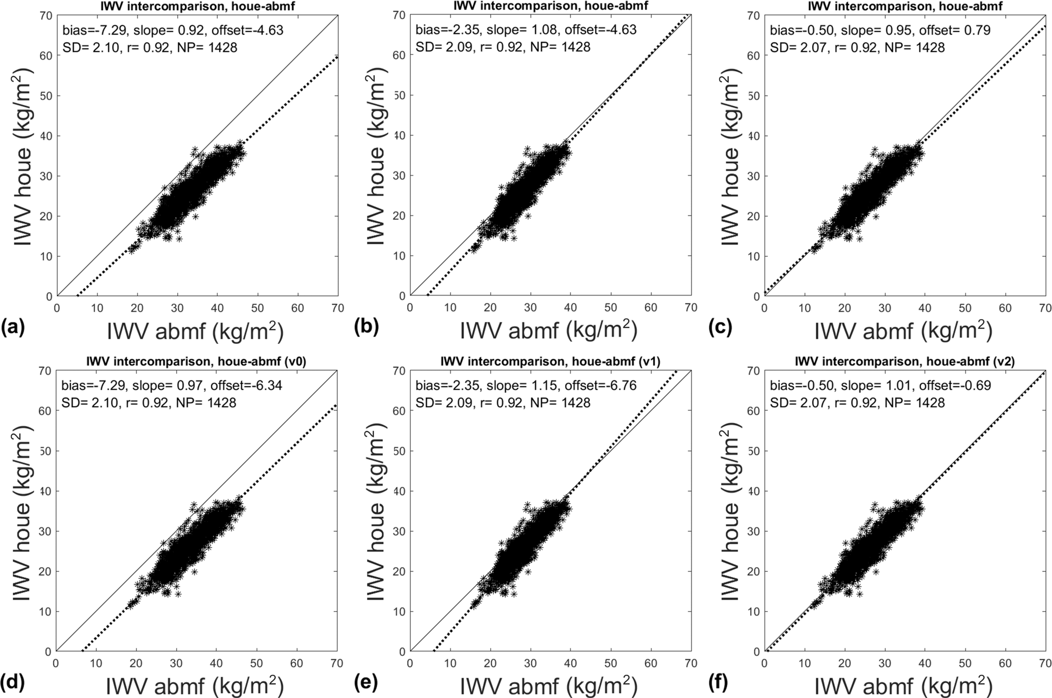
Figure 7Scatter plots of IWV observations from two GPS stations at different elevations (HOUE, 418 m, and ABMF, 15 m) before correction (a, d), after correction with a simple scaling factor model (b, e), and after correction with the proposed model fitted from a radiosonde climatology (c, f). The slope and offset parameters were either fitted by an ordinary least-squares method (a–c) or by the York et al. (2004) method accounting for errors in both coordinates (d–f). The data cover the period from 1 January to 29 February 2020, with a temporal resolution of 1 h.
Figure 8 presents the results for 105 inter-comparisons made of pairs of stations from the set of 15 stations of this network ordered by positive height differences, Δh>0. The plots compare the bias, offset, and slope for the uncorrected (v0) and the corrected (v1 or v2) data. Only the results from the York estimator are shown here. As expected, the uncorrected results show a general tendency towards larger negative biases, decreasing slope, and larger negative offset when Δh is increased. There are, however, some exceptions, namely the comparisons involving station CBE0 (altitude of 374 m), for which the biases and offsets are slightly less negative and the slopes are slightly farther from 1 than observed with the other stations, especially compared to station HOUE, which is located higher (418 m) and should thus have more pronounced effects. After correction with model v1, the biases and slopes are globally improved for all comparisons, while the offsets are unchanged, as expected with this model. The mean bias is reduced from −1.67 to −0.24 kg m−2, but some bias remains in the higher-altitude inter-comparisons involving HOUE (Fig. 8a). In contrast, model v2 achieves a better bias correction for HOUE (Fig. 8d). The results with model v2 also confirm the bias in the CBE0 that was already suspected from the uncorrected data. The problem with station CBE0 is further confirmed by the slope analysis, with model v2 indicating α2<1 for these inter-comparisons (Fig. 8e), and large positive offsets (Fig. 8f). The correction with model v1 is not able to lead to these conclusions because the slopes are globally overcorrected for many stations (Fig. 8b) and the offsets are unchanged (Fig. 8c). Figure 8e and f also detect scale errors and anomalous offsets for a number of other inter-comparisons, namely when Δh is close to zero.
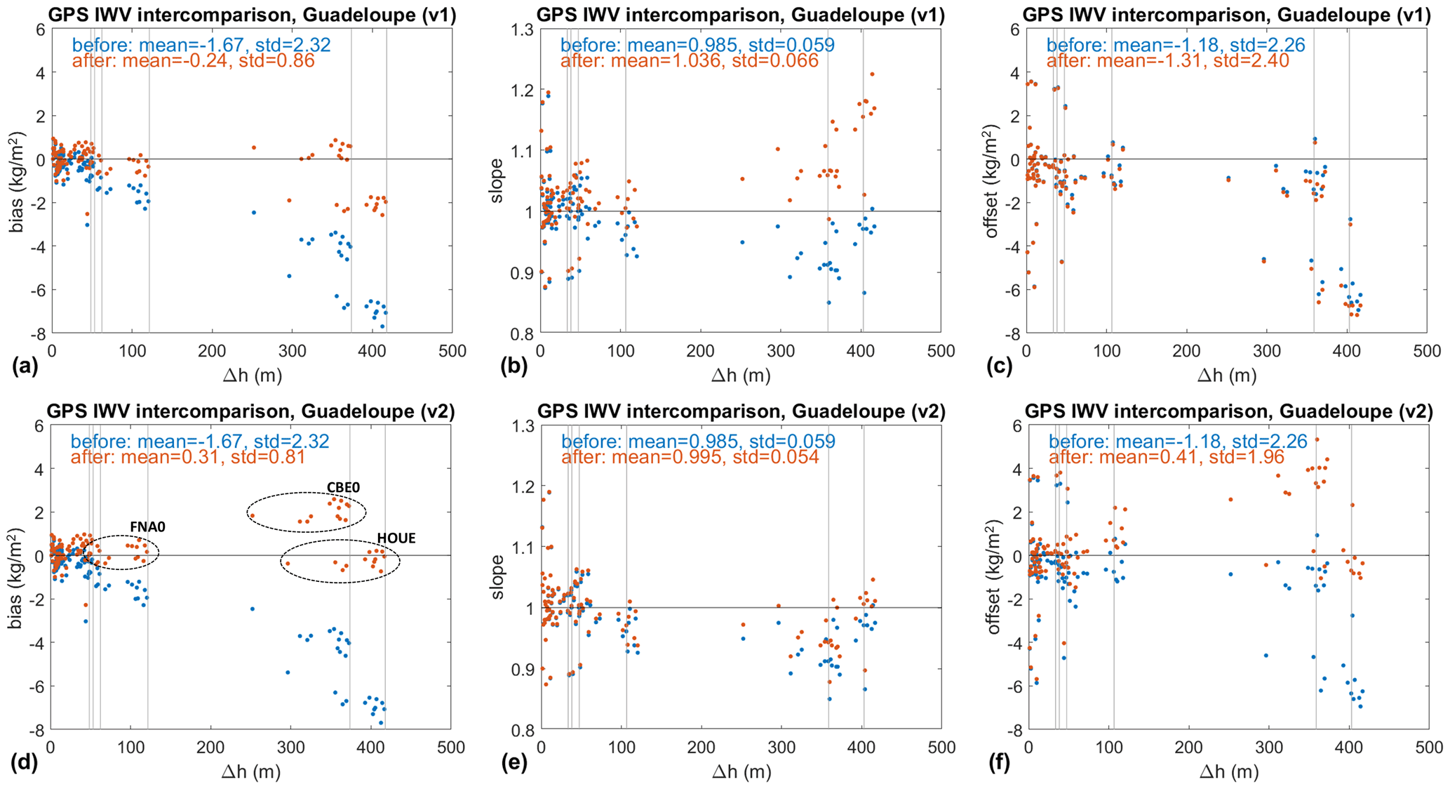
Figure 8Variation in (a, d) bias, (b, e) slope, and (c, f) offset estimated from pairs of GPS stations as a function of inter-station height difference, Δh. The blue dots correspond to the results before correction, and the red dots correspond to the results after correction, with (a–c) the scaling model, v1, and (d–f) the proposed model fitted from a radiosonde climatology, v2. The results include 105 inter-comparisons with positive height differences from a total of 15 GPS stations located over the Guadeloupe archipelago for the period from 1 January to 29 February 2020. The vertical grey lines indicate the stations that have elevations above 50 m, namely FNA0 (122 m), CBE0 (374 m), and HOUE (418 m), the comparisons of which are also highlighted by ellipses in Fig. 8d.
Figure 9 provides further insight into the consistency between stations, with significance tests computed according to the t-statistics given in Appendix C. It is evident that CBE0 has an anomalous positive IWV bias of about 2 kg m−2 compared to all other stations (Fig. 9a, red curve, well above the other curves), a slope that is too low (Fig. 9b, red curve below the other curves), and an offset that is too large (Fig. 9c). Figure 9b and c reveal a second outlying station, BOUL, with a slope that is too high (Fig. 9b, light blue curve, about 0.12 above the other stations) and an offset that is too low (Fig. 9c). These anomalies could not be detected from the uncorrected data or from the data corrected with model v1. Further investigation is needed to understand the issues in the IWV estimates for these two stations. Table 2 reports the median and the smallest absolute values for each station. Apart from stations CBE0 and BOUL, all other stations have median biases smaller than ±0.53 kg m−2, median slopes in the range 0.97–1.02, and median offsets smaller than ±0.77 kg m−2. These numbers demonstrate a very good consistency between IWV measurements retrieved from the different GPS stations of this network. The dispersion of results is believed to be due to station-dependent errors. The smallest absolute values quantify the best agreement between nearby GPS stations, which is <0.1 kg m−2 between all stations, except CBE0 which has a large bias, and BOUL which has a slope significantly different from 1.0.

Figure 9(a) Bias, (b) slope −1, and (c) offset estimated from all (210) pairs of GPS stations after correction with model v2 for the period from 1 January to 29 February 2020. The station names along the x axis refer to comparisons when the stations are in x, while the colour code indicates comparisons when the stations are in y. The bias is always reported as and the linear regression as . For example, station CBE0 has a positive bias (red curve) when considered in y, while it has a negative bias when considered in x. The comparison results from Fig. 8 were transformed using , and α′ and β′ according to Eqs. (B4a) and (B4b), when necessary.
Table 2Median values and smallest absolute values for the bias, slope (or slope −1), and offset of GNSS IWV inter-comparisons after correction for the height difference using the proposed model (v2). Data cover the period from 1 January to 29 February 2020. Slope and offset are estimated with the York et al. (2004) method. Bias and offset values that are significantly different from 0, and slope values that are significantly different from 1, are highlighted depending on their p value (∗ ≤0.05, ≤0.01). Two anomalous stations (BOUL and CBE0), with large bias and offset values and slope deviating from 1, are highlighted in bold.

4.2 GPS vs. MWR satellite inter-validation
GPS and MWR measurements of IWV are often used together for the inter-validation of the two techniques (Bock et al., 2007; Mears et al., 2015; Wentz, 2015; Ho et al., 2018). Microwave radiometer measurements are adversely affected by rain, whereas GPS measurements are not. On the other hand, the GPS IWV estimates have uncertainties linked with data processing models and conversion from propagation delay to IWV (Bock et al., 2013, 2021; Ning et al., 2016). The inter-comparison of both types of measurements is thus instructive for detecting and quantifying their mutual uncertainties.
Microwave radiometer measurements are traditionally made over the world's oceans, where they achieve their highest accuracy. The inter-comparison with GPS measurements is thus possible only for coastal stations and stations located on small islands. Although the MWR data are missing over land and over the island's footprint, due to “land contamination”, the high-resolution () of the RSS v7.0 data set used here (Mears et al., 2015) allows us to get enough valid measurements for comparison with the GPS stations on the Guadeloupe archipelago discussed in Sect. 4.1. Table 3 shows the mean distance between the GPS stations and the nearest MWR satellite grid points within the 7×7 pixels surrounding each station. On average over all stations, the mean distance is 33.6 km for AMSR2, 82.3 km for F18, 26.9 km for GMI, and 37.6 km for Windsat. The difference in distance is due to the difference of footprints of the satellite instruments, F18 having the largest footprint (69 km×43 km) and GMI the smallest (18 km×11 km). For the inter-comparison, MWR IWV data from the 7×7 pixels are interpolated to the location of the GPS sites by a Delaunay triangulation method (Press et al., 2007) and corrected vertically using the same method as for the GPS–GPS comparison discussed in Sect. 4.1. The height difference is here equal to the height of the GPS station, since the MWR data are valid on the mean sea level. The bias, slope, and offset parameters are derived as in the GPS–GPS comparison. The regression with the York et al. (2004) method needs to correctly specify the uncertainties of the measurements from the two data sets or at least to correctly represent the ratio of their mean uncertainties (see Appendix C). As mentioned above, the formal error rescaled by a factor of 5 is used for GPS. For MWR, we surmise that the horizontal interpolation from the gridded data will introduce some representativeness difference with the GPS point measurements that we should take into account. We first computed the standard deviation of all valid IWV values from the 7×7 pixels. It amounted to ∼2.2 kg m−2 on average over all sites and satellites. These values seemed too high to be used directly as a measure of uncertainty of the MWR data. However, the variations over time of the standard deviation are thought to correctly reflect the changes in the local atmospheric state, weather conditions, and measurement noise. In a second step, we made a three-way error analysis between GPS, MWR, and ERA5 IWV data, following O'Carroll et al. (2008). This was done with the GPS station BCON on Barbados (Bock et al., 2021). For this station, the number of valid MWR pixels was higher than at all other sites of the Caribbean GPS network, with an average of 46 valid pixels out of 49. This comparison is thus believed to provide a good estimate of the precision of the MWR data with negligible representativeness errors. We found the following standard error estimates for the three data sets: σGPS=1.06 kg m−2, σMWR=0.67 kg m−2, and σERA5=1.82 kg m−2 for AMSR2. Nearly similar values were found for the other satellites. According to these numbers, the GPS IWV data are slightly noisier than the MWR data, which seems plausible, although the MWR and ERA5 standard errors might be slightly underestimated given that MWR radiances are assimilated into ERA5, i.e. errors are correlated. Finally, we rescaled the GPS formal errors and the MWR standard deviations to match these three-way error values on average for each satellite. The resulting “measurements errors” were then used in the York fit.
Table 3Mean distance between GPS stations and the nearest MWR satellite grid-point within the 7×7 box surrounding each station (MWR grid resolution ). Values are given in kilometres. NA stands for not available.
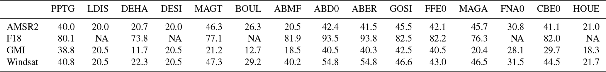
Figure 10 shows the results of the GPS–MWR comparisons, where the bias, slope, and offset parameters were retrieved for the whole year 2020. The number of collocations here is much smaller than for the GPS–GPS comparisons (between 200 and 400 for the GPS–MWR comparisons compared to nearly 8000 for the GPS–GPS comparisons over the full year). The median GPS–GPS results for the full year are superposed to emphasize the high correlation with the GPS–MWR inter-comparisons (the Pearson correlation coefficients reported in each plot). Regarding the biases especially, the variations from station to station are about ±0.5 kg m−2 (if we except CBE0) from both inter-comparisons. They are thought to be GPS station-specific errors (due to, e.g. multipath and/or field of view limitations). The large bias in CBE0 is confirmed with the MWR validation, but station BOUL does not appear to be an outlier here (for this station, the slope and offset estimates computed over the full year are closer to normal values, but inspection of monthly statistics revealed a drift throughout the year, the origin of which is not explained so far as no equipment change could be incriminated). All three versions of the comparisons also reveal a systematic mean bias between GPS and MWR IWV data of about 0.7 kg m−2 (0.67 kg m−2 with respect to AMSR2), with GPS being drier than MWR. A similar mean bias was previously observed by Mears et al. (2015) on global long-term averages including more GPS sites and satellites. Whether this bias is imbedded in the GPS or MWR retrievals is not clear at the moment. The mean difference between the different satellite estimates is, comparatively, slightly smaller: AMSR2 and Windsat agree almost perfectly, while GMI has a slight moist bias of +0.2 kg m−2 compared to either AMSR2 or Windsat, and F18 has a slight dry bias of −0.4 kg m−2 compared to the AMSR2. The slope estimates show more scatter between sites and satellites, although the mean GPS–MWR values agree very well with the GPS–GPS values. Similar to the findings of Sect. 4.1, the classical correction (v1) does not preserve the slopes and leads to large overestimations for the stations at higher altitudes. Again, the new correction (v2) achieves almost perfect slopes for both the GPS–GPS and the GPS–MWR comparisons.
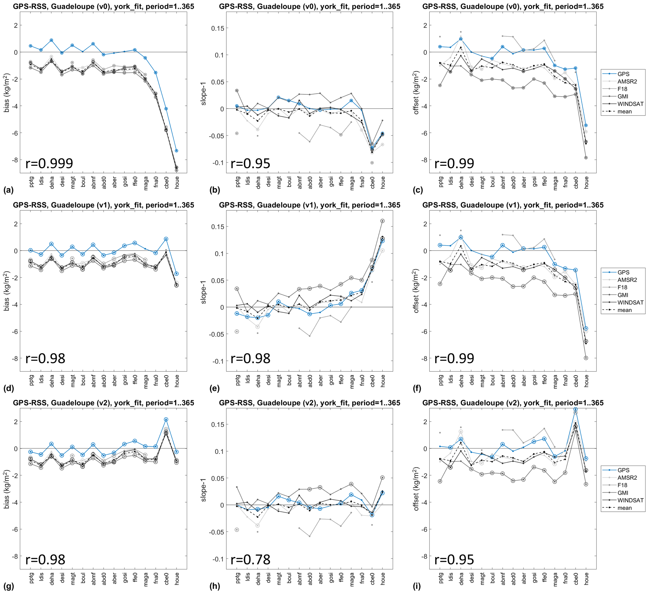
Figure 10Bias, slope, and offset results for GPS–GPS comparisons (the blue line shows median of all GPS comparisons from Fig. 9 except for the full year) and for GPS–MWR comparisons from four different satellites (AMSR2, F18, GMI, and WINDSAT; the dashed black line shows the mean of all satellite results) for the year 2020. Slope and offset are estimated with the York et al. (2004) method. Bias and offset values significantly different from 0 and slope values significantly different from 1 are marked with a circle (p value ≤0.01). Pearson correlation coefficients between GPS–GPS and mean GPS–MWR results are indicated in the lower left of each plot.
Following the IWV inter-comparisons, statistical tests (Appendix C) were applied to sort those comparisons that show biases and offsets that are significantly different from zero and slopes significantly different from one. Test results with p values <0.01 are highlighted in Fig. 10 for all comparisons. It can be noted that most biases (but not all slopes and offsets) are significant. Indeed, the standard errors for the latter parameters remain relatively high, despite a full year of data being used here. For example, several slopes of the GPS–F18 comparisons deviate notably from 1 but are not significant (mean standard error of 0.0193), whereas they are significant for the GPS–GPS inter-comparison (mean standard error of 0.0029). These results indicate that accurate vertical correction (model v2), correct specification of the measurement errors, and sample size are all crucial when diagnosing biases and scaling errors.
In this paper we have shown that the model traditionally used for the correction of the IWV difference due to the vertical displacement between observation sites has two shortcomings. First, it induces a bias in the slope estimate and correlatively in the offset estimate, with slopes being overestimated when the IWV measurements from the lower site are corrected (see, e.g. Fig. 10e). Second, it does not change the offset estimate, which remains generally close to the uncorrected bias value (Fig. 10a, c, and f). We have proposed an improved correction model (Eq. B8) based on two terms, fc and gc, which overcomes these limitations. This model relies on a multi-linear regression of slope and offset (Eq. B9) as a function of the height difference (Eqs. 5 and 6). We have shown that high-resolution radiosonde data are capable of providing accurate estimates of the parameters (ai,bi) of this model on a monthly basis. The correction model reduces the bias, slope, and offset to negligible mean errors (, , ) for height differences up 500 m, with a standard deviation smaller than 0.5 kg m−2. The errors are expected to increase slightly for larger height differences (e.g. we found , , for a height difference of 1000 m with the data from radiosonde station 78897). The method has been successfully applied to the correction of GPS IWV data from a network of stations in a tropical mountainous area, with altitudes ranging from the sea level up to more than 400 m. Corrected data were allowed to diagnose anomalous biases and scaling errors at two sites that could not be detected in the raw measurements or when the traditional correction method was applied. The method was also applied to inter-validation of IWV from satellite MWR measurements and GPS measurements in the same region. The corrected data confirmed the significant bias and anomalous slope for one of the GPS stations (CBE0, bias close to 2 kg m−2, and slope close to 0.98). The reason why the second station (BOUL) did not show up in this comparison is that the errors decreased over time, possibly linked with several equipment changes that were reported during 2020 at this site. Some dispersion was also observed between the four satellite data sets that were compared, with F18 showing more scatter as well as a smaller number of available collocations. We suspect that the larger footprint of the MWR instrument on board this satellite induced larger representativeness differences, since pixels located farther from the GPS stations have been used. F18 might also have slightly more land contamination than the other satellites do. However, when the results from the four satellites were averaged together, they were in very good agreement with the GPS-only results.
This study also emphasized the need for using a regression method that accounts for errors in both variables and for correctly specifying these errors. Not doing so is known from least-squares theory to result in biased slope and offset estimates, as well as biased standard errors and inconsistencies in subsequent significance tests. These issues are discussed in Appendix C (using Monte Carlo simulations) and illustrated in Sect. 4.1 for the case of the GPS–GPS inter-comparison. It is shown that the regression method of York et al. (2004) works well as soon as the ratio of the uncertainties in both variables is properly specified. Stated differently, it appears not to be necessary to provide absolute uncertainties but only relative ones. This is fortunate as the former are usually not known unless an absolute calibration technique is involved. In this study, we have successfully used a triple collocation method to estimate the relative errors in the GPS and MWR data, using ERA5 as the third data set. This approach provides generally satisfying results as long as the representativeness errors in all data sets are small or at least similar (Stoffelen, 1998; O'Carroll et al., 2008). In our case, the MWR and ERA5 have similar spatial resolutions, which may induce representativeness errors of similar magnitudes compared to the GPS observations (which are of a more local nature). We also attempted to combine GPS, satellite MWR, and radiosonde observations, but the triple collocation failed in this case. However, the combination of co-located GPS, radiosonde, and ground-based MWR measurements from the Barbados Cloud Observatory during the EUREC4A campaign worked well. In this case, we found the following error estimates: σGPS=0.93, σRS=0.65 and σMWR=1.53 kg m−2. This new estimate for the GPS errors is fairly consistent with the one found with the satellite MWR and ERA5 data reported in Sect. 4.2. It is also consistent with the estimate reported by Cimini et al. (2012) of 0.94 kg m−2. The other two errors seem plausible as well, especially the higher value for the ground-based MWR data that were shown to contain excessive noise during the first weeks of the campaign (Bock et al., 2021).
The improved vertical correction method described in this paper can be easily applied to any other region for which high-resolution vertical profiles of water vapour are available. Such profiles can be provided by radiosonde observations, numerical weather model outputs, or reanalyses. A few additional trials showed that very good results are still achieved with a vertical resolution of 100 m (e.g. bias error smaller than 0.1 kg m−2). In this study, the model parameters have been derived on a monthly basis, and they seem to be well adapted to correct data sets that cover at least 1 month of measurements. We also tested separate model adjustments and corrections for the 00:00 and 12:00 UTC profiles, but the results were not significantly different. In the future, we plan to derive the model parameters on a global grid from the ERA5 reanalysis that provides a stable and accurate climatology of the water vapour distribution. The global correction grid will be useful to provide more accurate inter-comparisons and inter-validations of global IWV data sets from various techniques.
The distribution of water vapour density in the atmosphere is generally highly variable but may be approximated by the following equation:
where γ>0 is the mean vertical decay rate of water vapour, also sometimes expressed as the inverse of the water vapour scale height, , ρ0 is the ground-level water vapour density, and h is the geometric height. Standard values for Hv and ρ0 are Hv=2 km and ρ0=7.5 g m−3 or alternatively m−1 (ITU, 2017).
It follows from Eq. (A1) that the IWV above a height hA is simply
The IWV in the layer in between two stations, A and B, at heights hA and hB is written as follows:
Equation (A3) can be used to correct the IWV measurements from station A to conform to the height of station B in an additive way: , where IWVA=IWV(hA). Combining Eqs. (A2) and (A3) shows that the correction is actually multiplicative in nature:
Here we can define fc(Δh) as the correction factor which (applied to IWVA) conforms to the height hB:
where is the height difference between station A and station B.
When is small (or more rigorously when ), Eq. (A5) can be approximated by , which leads to a widely used form of the IWV correction (Bock et al., 2005; Morland et al., 2006a, b; Buehler et al., 2012):
Equation (A6) has traditionally been used to estimate γ from the IWV observations at different heights, e.g. for two stations at heights hA and hB:
which expresses the idea that γ represents the fractional IWV variation over a height Δh (Bock et al., 2005). The range of validity for the approximate formulations expressed by Eqs. (A6) and (A7) to hold can be estimated from the condition , which leads to m if we use km. For larger height differences, it is recommended to use the exact formulations (Eqs. A4 and A8):
Let us assume that we have n observations, (xi,yi), i=1…n, corresponding to paired measurements of the same physical quantity coming from the same instrument at two different sites or from two different instruments at the same site. The difference in the observation conditions is assumed to lead to a bias, Δ, and a scaling error that can be represented by a linear fit slope, α, and offset, β, defined as follows:
where μx and μy are the sample means of x and y and the slope and offset parameters are derived from the linear regression model:
Thanks to the linearity of the mean operator, Eq. (B2) relationship is also verified for the means as follows:
Note that since {xi} and {yi} are both obtained from measurements, they are usually both subject to errors. There are robust methods in the literature to optimally estimate α and β in the presence of errors in both variables (e.g. Mandel, 1984; Macdonald and Thompson, 1992; York et al., 2004). It should also be noted that, depending on which of x and y is considered as the reference, the opposite relationship may sometimes be used, , which relates to Eq. (B2) by
Note that Eqs. (B4a) and (B4b) are in general not verified when the estimation method does not account for errors in both variables.
Equations (B1) and (B3) recall that the parameters Δ, α, and β are inter-related through μx and μy. It is instructive to discuss the different cases of interest for the interpretation of experimental results. These cases are described below and illustrated in Fig. B1.
-
Case no. 1: α=1. In this case, the two observation series only have a bias and no scaling error, and it follows from Eqs. (B1) and (B3) that and β=Δ.
-
Case no. 2: α>1. In this case, the two series have a scaling error, where the range of yi values is larger than the range of xi values. It also follows from Eqs. (B1) and (B3) that β<Δ. Depending on the sign of Δ there is an additional constraint or not on β.
- (a)
If Δ>0, then β can be either positive or negative, with β<Δ.
- (b)
If Δ<0, then β can be only negative, i.e. .
- (a)
-
Case no. 3: α<1. In this case, the two series have a scaling error, where the range of yi values is smaller than the range of xi values, and it follows from Eqs. (B1) and (B3) that β>Δ. Again, there may be an additional constraint on β.
- (a)
If Δ>0, then β can be only positive, i.e. ,.
- (b)
If Δ<0, then β can be either positive or negative, with β>Δ.
- (a)
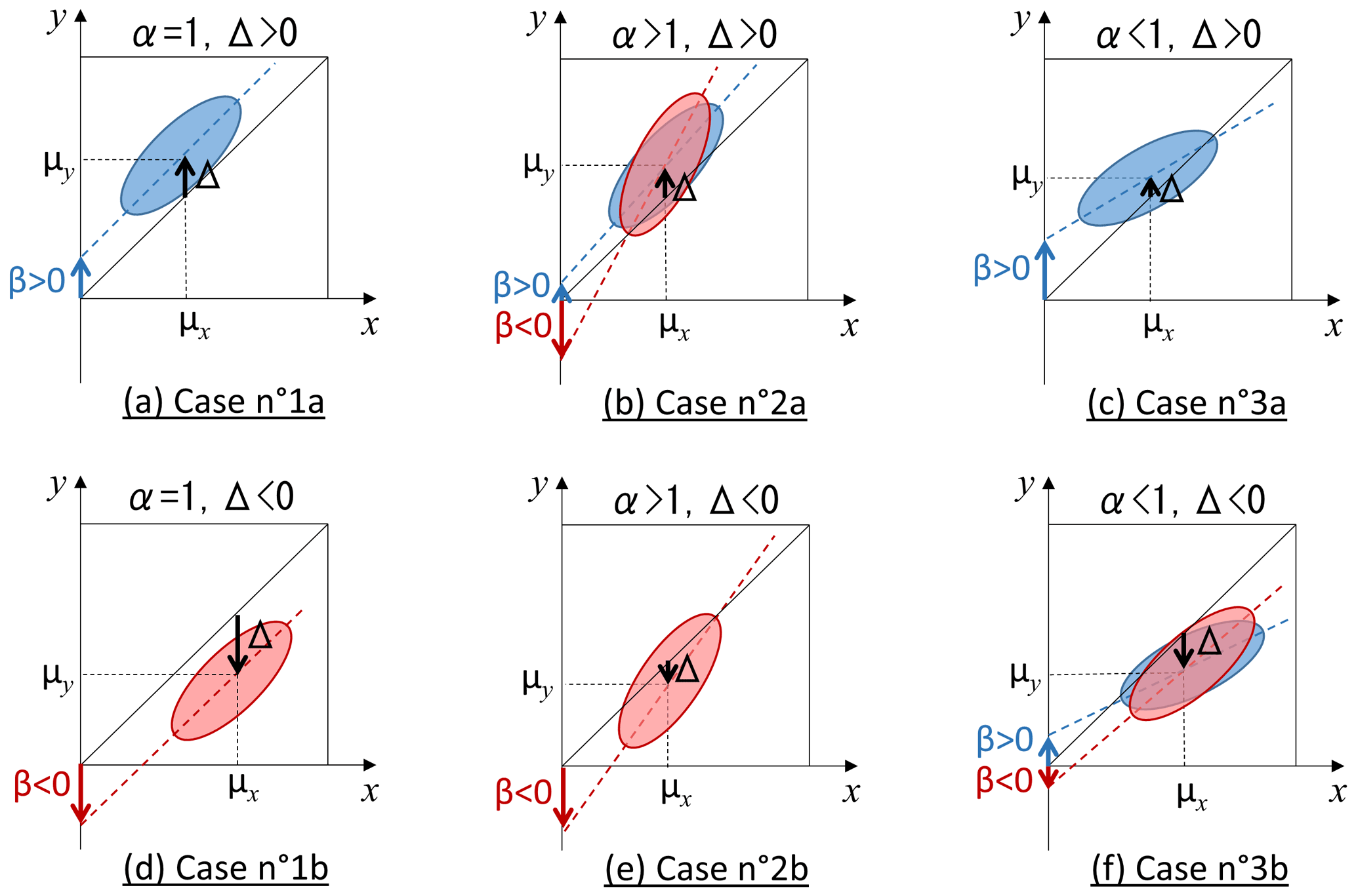
Figure B1Illustration of different cases of paired observations with perfect scaling (α=1), imperfect scaling (α>1 or α<1), and positive or negative bias (Δ>0 or Δ<0). Each case has a different implication on the offset parameter β obtained from a linear regression with the model . The regression lines are shown as dashed lines, with red indicating negative offsets and blue positive offsets. The 1:1 lines are shown as solid black lines. The distributions of data around the regression lines are represented schematically by the red and blue ellipses.
Let us now analyse the impact of applying a rescaling of the reference series, {xi}, in order to correct it for difference in the observation conditions with respect to the tested series {yi}. We denote the corrected series by {xi,c}, with . In the case of IWV vertical correction, the scaling factor fc could be computed from Eq. (A5) under the hypothesis of a vertical distribution of water vapour following an exponential law. The bias, slope, and offset parameters after correction are denoted, respectively, as Δc, αc, and βc, and are written as follows:
Equations (B5) and (B6) follow from the fact that must hold for every μx. A crucial question is to check if this correction method can achieve a perfect bias correction and scaling simultaneously, i.e. Δc=0 and αc=1.
Let us first check the conditions for achieving a zero bias, Δc=0. This result is achieved if and only if . From this condition, it follows that . The only possibility to simultaneously achieve Δc=0 and αc=1 is actually that α=1, i.e. when the data initially only have a bias but no scaling error. In all other cases, the final slope will be different from one, and it can be either larger or smaller than the initial slope, meaning that in some cases the slope can be degraded (getting farther from one). These situations again depend on the initial values of α and Δ.
-
Case no. 1. If Δ>0, then αc<α. If, in addition, α<1, then , i.e. the slope is degraded. If, instead, α>1, then αc<α can lead to an improvement in the slope, but there is no guarantee that αc will be close to 1.
-
Case no. 2. If Δ<0, then αc>α. If, in addition, α>1, then , i.e. the slope is degraded. If, instead, α<1, then αc>α can lead to an improvement in the slope, but there is no guarantee that αc will be close to 1.
The above analysis shows that, except when α=1, the final slope will be different from 1, and in some cases, depending on the sign of the initial bias, it will be degraded.
Let us now check the conditions for achieving a unity slope, αc=1. This result is achieved if and only if fc=α. From there it can be seen that Δc=β, meaning that the sign and magnitude of the final bias will depend on the sign and magnitude of the initial offset. Unless β=0, the final bias will generally be different from zero; i.e. it is in general not possible to achieve a zero bias if the reference data are corrected by a simple scaling factor that would achieve a final slope of 1.
Instead of a simple rescaling correction model, we propose using a linear correction model that includes both a scaling factor, fc, and an intercept, gc:
For our application to IWV vertical correction, both fc and gc would depend on the height difference, Δh. Following the same reasoning as for the simple scaling model, it is straightforward to show that the condition to achieve both a zero bias, Δc=0, and a unity slope, αc=1, after correction is written as follows:
Indeed, substituting Eq. (B9) into Eq. (B8) and expressing the bias and the linear fit equation , after correction we find Δc=0, αc=1, and βc=0, which is the desired result.
The classical straight-line fitting problem can be formalized as follows. Let us assume the linear model
where Y is the response variable, x the independent variable, α and β the slope and intercept, and εY a random variable of zero mean and variance , representing the error in Y. When x is known without error, the ordinary least-squares (OLS) solution is found by minimizing the sum of squared errors, , where and is the predicted value from the fitted line. In this case, the errors represent the vertical distance of the best-fit line to the data points. The OLS solution for α and β has a simple analytical formulation (Walpole et al., 2012):
The variance of the OLS estimators is given by the following equations (Walpole, 2012):
An unbiased estimate of is given by the following equations (Walpole, 2012):
From there, it is customary to compute the standard errors of the estimates as follows:
Assuming that the errors εY,i are normally distributed, it follows that the estimators αOLS and βOLS are also normally distributed and that is a chi-squared variable with n−2 degrees of freedom. Hypothesis testing of the fitted parameters is then done using the following statistics:
which both have t distributions with n−2 degrees of freedom. In Eqs. (C6a) and (C6b), α0 and β0 are the values assumed in the null hypotheses. Typically, one wants to test H0: αOLS=1 against H1: αOLS≠1 and H0: βOLS=0 against H1: βOLS≠0. The associated p values are then computed from the t cumulative distribution function (CDF):
When x is observed with error, a second observing equation applies:
where the observed quantity X of the unknown variable x now contains a random error εX and the OLS solution (Eq. C2) is no longer optimal. Indeed, the slope estimate will typically have negative bias (see Draper and Smith, 1998, Eq. 3.4.10, for an expression of the bias), and this will bias the intercept estimate in return.
The solution of the regression of Y on X with errors in both variables can be found by minimizing the sum of squared errors in both variables, i.e. , where w(xi) and w(yi) are the weights of the observations and and are the predicted values. Weights have been included here to follow the formalism of York et al. (2004). They would typically be computed from the assumed uncertainties, u, in the measurements, e.g. and . Note that in the special case of unit weights, the solution is the straight line that minimizes the sum of the squares of the perpendicular distances to the observed points (Macdonald and Thompson, 1992). Finding the solution to this problem is not straightforward, and many different and often approximate solutions have been proposed in the literature (see, e.g. the discussion in Press et al., 2007). In this work, we use the iterative algorithm approach proposed by York et al. (2004), which also includes equations for the standard errors of the fitted parameters. The equations are more complex than those of the OLS solution and will not be repeated here. The standard errors of the York estimators can be likewise used with Eqs. (C6) and (C7) for hypothesis testing. However, here we want to emphasize that the formulations of the standard errors given by York et al. (2004) need to be rescaled by the goodness of fit factor , where SSE is the residual sum of squares given above. This rescaling is important to retrieve realistic values of the standard errors and thus the test statistics and the subsequent p values. If the uncertainties in the measurements have been properly specified, this quantity should be close to 1.
In addition, it is useful to describe how the bias estimates can be tested. We especially want to test the null hypothesis (H0: Δ=0) against H1: Δ≠0, where Δ is computed as . The difficulty here is with standard error of Δ when both variables have errors. It can be shown that the mean and variance of the Δ estimator are and , respectively. The problem here is that and are unknown. It may be conjectured that is a proper estimator of the variance of Y−X, with and , and that may be used as an estimator of . However, it can be shown that and that the first term is typically dominant over the latter two, i.e. this estimator of is biased. Instead, we propose using Eq. (C4) as an estimator of and a similar estimator for :
where is the predicted value for xi. It can be shown that and . Since in our applications α is usually close to 1 and the two error variances () are comparable, both estimators will only depart slightly from . As a consequence, we propose averaging the two estimates and use
as an estimator of . Note that the OLS and York estimators predict different values of because and depend on the estimated values of α and β. The test statistic and subsequent p value for Δ can be computed in a similar manner to what was used for α and β, although the statistic does not exactly follow a t distribution in this case.
The performance of the OLS and York regression methods have been evaluated based on Monte Carlo tests. The main goals were to evaluate (i) the impact of errors in x on the OLS estimator, (ii) the impact of misspecification of the errors in the two variables with the York estimator, and (iii) the performance of the test statistic for the bias. We simulated m=105 data sets, each composed of n=41 pairs of observations, (xi,yi), i=1…n, where xi=10…50 by a step of 1 plus a random value from a normal distribution, , and plus a random value from a normal distribution, , where is the true (noise-free) value of xi. Table C1 presents the results for different cases where the true noise variances, and , were changed and the assumed variances, and , were either correctly specified or not (note that the latter are used only in the York fit). All of these simulations were run with α=1 and β=0. We also run simulations for other values of α and β, but the conclusions were unchanged; e.g. with α=0.8 and β=5.0 we did not observe any significant difference in the results compared to those presented in Table C1. Note that the SE values for Δ reported in Table C1 were computed with the York estimates of α and β. We observed that they were consistent with the values computed with the OLS estimates to 0.01 or better (OLS values greater than York values) and consequently led to the same hypothesis test results on average.
Table C1Monte Carlo tests of linear regression using the ordinary least-squares (OLS) and the York et al. (2004) method. In all simulated cases, the true slope is 1 and true offset is 0. Noise is simulated in both variables according to the standard deviation values indicated in the first two columns. Each data set was run for 105 simulations. The OLS method assumes noise is present only in the y variable. The York method accounts for errors in both variables, with uncertainties specified in the third and fourth columns. The other columns report the mean and standard deviation (SD) of estimated parameters (bias, slope, and offset) and their mean standard errors (SE). The column “p<0.05” indicates the fraction of results that have p values smaller than 0.05. The expected value for the latter is 0.05. Mean values and p<0.05 values that differ significantly from the expected values are highlighted in bold.
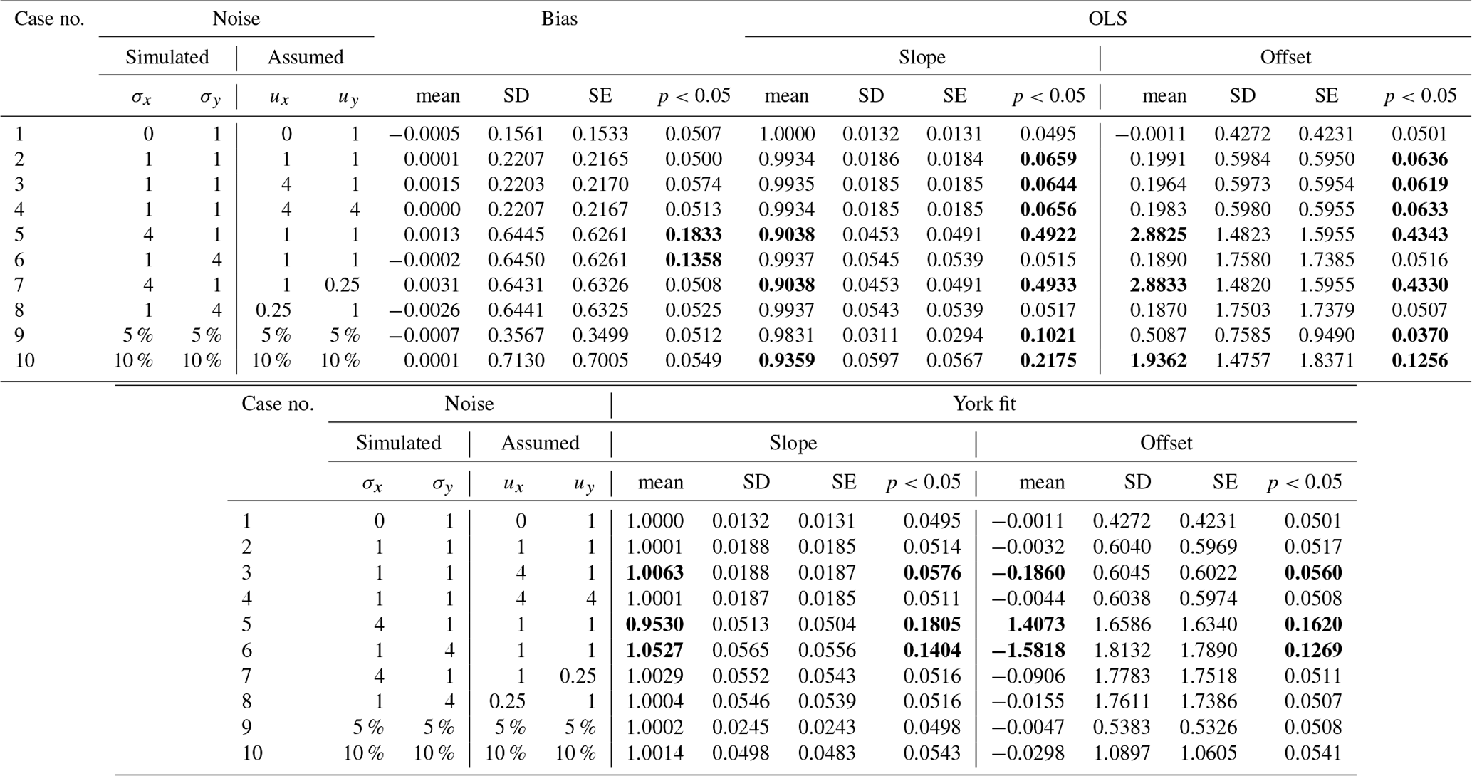
The performance of the estimators was assessed in terms of bias (difference between the mean estimate and the truth), variance (the consistency between the observed standard deviation, SD, and the mean standard error, SE), and the correctness of the 5 % significance level (the value p0.05 reported in Table C1 is the fraction of simulations with p values <0.05). The results are summarized below.
-
Where and no errors are simulated in x (case no. 1), the OLS and York methods yield identical results (mean, SD, SE, p0.05).
-
Where , the OLS estimates of slope and offset are biased (αOLS<1 and βOLS>0) and the magnitudes of the biases depend on the strength of the noise.
-
When σX=1 (case nos. 2, 3, 4, 6, 8), the biases are small: αOLS≈0.993, βOLS≈0.19, and p0.05≈0.06.
-
When σX=4 (case nos. 5, 7), the biases are larger: αOLS≈0.90, βOLS≈2.9, and p0.05≈0.5.
-
When σX is proportional to X (case nos. 9, 10), the biases take intermediate values: αOLS=0.93–0.98, βOLS=0.5–1.9, and p0.05=0.1–0.2.
-
When σY>σX (case nos. 6, 8), the mean values are unchanged, SD and SE increase, and p0.05 is improved (compare, e.g. case nos. 2 and 6).
-
-
Where , the York estimates are unbiased in all cases, except when the uncertainties are misspecified and are dissimilar in both variables.
-
When (case nos. 3, 5, 6), the biases amount to , , and p0.05=0.14–0.18 in case nos. 5 and 6, but they are much smaller in case no. 3.
-
When (case nos. 7, 8), all the biases vanish, but the specified uncertainties are smaller than the true errors.
-
-
The standard errors are consistent with the standard deviations in all cases. They increase when the noise increases. Note that the standard errors are relatively large in these simulations because the samples contain only n=41 values. Increasing n by a factor of 10 (consistent with the GPS–MWR comparisons of Sect. 4.2) would decrease SE by a factor of 10. A reduction of the SE would also imply that some of the slope and offset biases become significant (e.g. in case no. 3).
-
The bias estimator, , is “unbiased” in all cases (mean ≈ true value) and its SE estimator is consistent with the standard deviation (this confirms the validity of the SE estimator given by Eq. C10) with only a small bias when the noise variances are dissimilar (case nos. 5, 6: SE ≈ 0.62 compared to SD=0.64) and a subsequent impact on the p0.05 probabilities (p0.05=0.13–0.18).
Note that even when is constant, the OLS estimators and subsequent test statistics are biased.
Figure C1 shows the distributions of the slope, offset, and p values from the hypothesis tests for case nos. 5 and 7. The shapes of the distributions of the slope and offset resemble non-central t distributions. Note the biases of the OLS estimators in both cases and the bias in the York estimators only in case no. 5. The distributions of the p values are expected to be flat (equal probability for all p values), which is verified for the York fit in case no. 7 and all other simulated cases, except for case nos. 5 and 6 and to a lesser extent case no. 3 (where the error ratios are misspecified). In case no. 5 (shown in Fig. C1), it is seen that the small p values have larger probability, which indicates that an excessive number of slope and offset estimates are biased. This happens more often with the OLS estimator.
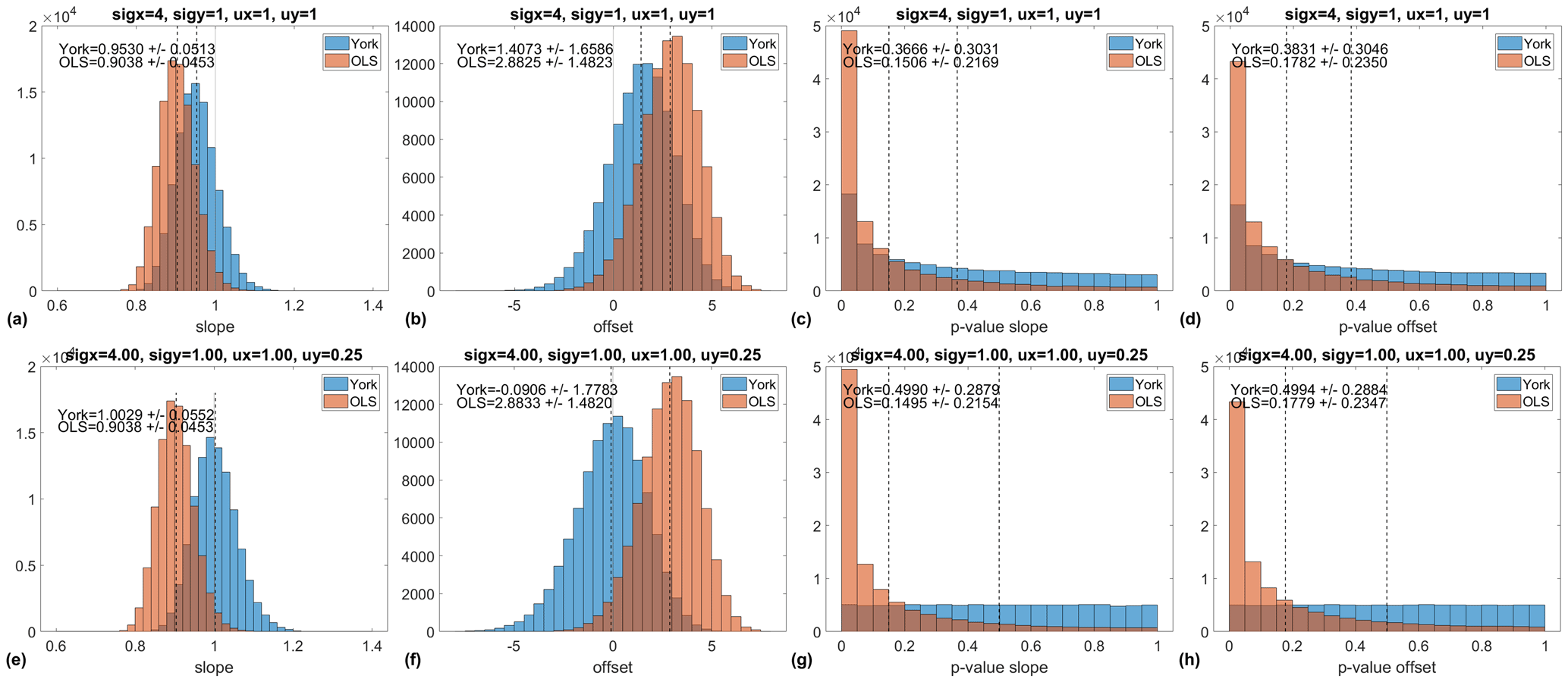
Figure C1Monte Carlo tests of linear regression using the ordinary least-squares (OLS) and the York et al. (2004) methods. The plots show the distributions of slope, offset, and respective p values from the hypothesis tests (H0: slope equal to 1; H0: offset equal to zero). The dotted vertical lines indicate the mean values. Mean and standard deviation are reported in each plot. The true slope is 1, and the true offset is 0. Panels (a)–(d) correspond to case no. 5 from Table C1, and panels (e)–(h) correspond to case no. 7. Each case is computed from 105 simulations (see Appendix C for further details).
The high-resolution radiosonde data used in this work were retrieved from the University of Wyoming web site (http://weather.uwyo.edu/upperair/bufrraob.shtml, last access: 29 September 2022; University of Wyoming, 2022). The GPS IWV data are available from AERIS, the French national data and service portal for the atmosphere (https://www.aeris-data.fr/, last access: 29 September 2022), under DOI https://doi.org/10.25326/79 (Bock, 2020). The satellite MWR data are freely available via ftp from https://www.remss.com/missions/ (last access: 29 September 2022; Wentz et al., 2012) after registration.
OB initiated the study, proposed the new correction method, performed the comparisons, and wrote the paper. PB and CM processed the GPS and MWR data used in this work, respectively. All three authors contributed to the interpretation and discussion of the results.
The contact author has declared that none of the authors has any competing interests.
Publisher's note: Copernicus Publications remains neutral with regard to jurisdictional claims in published maps and institutional affiliations.
This article is part of the special issue “Analysis of atmospheric water vapour observations and their uncertainties for climate applications (ACP/AMT/ESSD/HESS inter-journal SI)”. It is not associated with a conference.
The authors would like to thank Guillaume Gamelin (Meteo-France) for providing assistance by quality checking the high-resolution radiosonde data of the station at Le Raizet, Guadeloupe, France. The authors are grateful to AERIS (https://www.aeris-data.fr/, last access: 29 September 2022), the French data and service centre for atmosphere, for providing the ERA5 reanalysis data. This work was developed in the framework of the VEGAN project supported by the CNRS programme LEFE/INSU.
This research has been supported by the Centre National de la Recherche Scientifique (LEFE/IMAGO/VEGAN).
This paper was edited by Martina Krämer and reviewed by Tobias Nilsson and two anonymous referees.
Bedka, S., Knuteson, R., Revercomb, H., Tobin, D., and Turner, D.: An assessment of the absolute accuracy of the Atmospheric Infrared Sounder v5 precipitable water vapor product at tropical, midlatitude, and arctic ground-truth sites: September 2002 through August 2008, J. Geophys. Res., 115, D17310, https://doi.org/10.1029/2009JD013139, 2010.
Bennartz, R., Höschen, H., Picard, B., Schröder, M., Stengel, M., Sus, O., Bojkov, B., Casadio, S., Diedrich, H., Eliasson, S., Fell, F., Fischer, J., Hollmann, R., Preusker, R., and Willén, U.: An intercalibrated dataset of total column water vapour and wet tropospheric correction based on MWR on board ERS-1, ERS-2, and Envisat, Atmos. Meas. Tech., 10, 1387–1402, https://doi.org/10.5194/amt-10-1387-2017, 2017.
Bock, O.: Reprocessed IWV data from ground-based GNSS network during EUREC4A campaign, EUREC4A [data set], https://doi.org/10.25326/79, 2020 (data available at: https://www.aeris-data.fr/, last access: 29 September 2022).
Bock, O., Keil, C., Richard, E., Flamant, C., and Bouin, M. N.: Validation of precipitable water from ECMWF model analyses with GPS and radiosonde data during the MAP SOP, Q. J. Roy. Meteor. Soc., 131, 3013–3036, https://doi.org/10.1256/qj.05.27, 2005.
Bock, O., Bouin, M.-N., Walpersdorf, A., Lafore, J. P., Janicot, S., Guichard, F., and Agusti-Panareda, A.: Comparison of ground-based GPS precipitable water vapour to independent observations and Numerical Weather Prediction model reanalyses over Africa, Q. J. Roy. Meteor. Soc., 133, 2011–2027, https://doi.org/10.1002/qj.185, 2007.
Bock, O., Bosser, P., Bourcy, T., David, L., Goutail, F., Hoareau, C., Keckhut, P., Legain, D., Pazmino, A., Pelon, J., Pipis, K., Poujol, G., Sarkissian, A., Thom, C., Tournois, G., and Tzanos, D.: Accuracy assessment of water vapour measurements from in situ and remote sensing techniques during the DEMEVAP 2011 campaign at OHP, Atmos. Meas. Tech., 6, 2777–2802, https://doi.org/10.5194/amt-6-2777-2013, 2013.
Bock, O., Willis, P., Wang, J., and Mears, C.: A high-quality, homogenized, global, long-term (1993–2008) DORIS precipitable water data set for climate monitoring and model verification, J. Geophys. Res.-Atmos., 119, 7209–7230, https://doi.org/10.1002/2013JD021124, 2014.
Bock, O., Bosser, P., Flamant, C., Doerflinger, E., Jansen, F., Fages, R., Bony, S., and Schnitt, S.: Integrated water vapour observations in the Caribbean arc from a network of ground-based GNSS receivers during EUREC4A, Earth Syst. Sci. Data, 13, 2407–2436, https://doi.org/10.5194/essd-13-2407-2021, 2021.
Bokoye, A. I., Royer, A., O'Neill, N. T., Cliche, P., McArthur, L. J. B., Teillet, P. M., Fedosejevs, G., and Theriault, J.-M.: Multisensor analysis of integrated atmospheric water vapor over Canada and Alaska, J. Geophys. Res., 108, 4480, https://doi.org/10.1029/2002JD002721, 2003.
Bokoye, A. I., Royer, A., Cliche, P., and O'Neill, N.: Calibration of sun radiometer–based atmospheric water vapor retrievals using GPS meteorology, J. Atmos. Ocean. Tech., 24, 964–979, 2007.
Buehler, S. A., Östman, S., Melsheimer, C., Holl, G., Eliasson, S., John, V. O., Blumenstock, T., Hase, F., Elgered, G., Raffalski, U., Nasuno, T., Satoh, M., Milz, M., and Mendrok, J.: A multi-instrument comparison of integrated water vapour measurements at a high latitude site, Atmos. Chem. Phys., 12, 10925–10943, https://doi.org/10.5194/acp-12-10925-2012, 2012.
Christensen, R.: Advanced linear modeling: multivariate, time series, and spatial data nonparametric regression and response surface maximization, 2nd edn., Springer, New York, https://doi.org/10.1007/978-1-4757-3847-6, 2001.
Cimini, D., Pierdicca, N., Pichelli, E., Ferretti, R., Mattioli, V., Bonafoni, S., Montopoli, M., and Perissin, D.: On the accuracy of integrated water vapor observations and the potential for mitigating electromagnetic path delay error in InSAR, Atmos. Meas. Tech., 5, 1015–1030, https://doi.org/10.5194/amt-5-1015-2012, 2012.
Courcoux, N. and Schröder, M.: The CM SAF ATOVS data record: overview of methodology and evaluation of total column water and profiles of tropospheric humidity, Earth Syst. Sci. Data, 7, 397–414, https://doi.org/10.5194/essd-7-397-2015, 2015.
Dousa, J. and Elias, M.: An improved model for calculating tropospheric wet delay, Geophys. Res. Lett., 41, 4389–4397, https://doi.org/10.1002/2014GL060271, 2014.
Draper, N. R. and Smith, H.: Applied Regression Analysis, Wiley Series in Probability and Statistics, 3rd edn., Wiley-Interscience, ISBN: 978-0-471-17082-2, 1998.
Du, J., Kimball, J. S., and Jones, L. A.: Satellite microwave retrieval of total precipitable water vapor and surface air temperature over land from AMSR2, IEEE T. Geosci. Remote, 53, 2520–2531, https://doi.org/10.1109/TGRS.2014.2361344, 2015.
Edland, S. D.: Bias in slope estimates for the linear errors in variables model by the variance ratio method, Biometrics, 52, 243–248, 1996.
Ho, S.-P., Peng, L., Mears, C., and Anthes, R. A.: Comparison of global observations and trends of total precipitable water derived from microwave radiometers and COSMIC radio occultation from 2006 to 2013, Atmos. Chem. Phys., 18, 259–274, https://doi.org/10.5194/acp-18-259-2018, 2018.
Hocking, R. R.: A Biometrics Invited Paper. The analysis and selection of variables in linear regression, Biometrics, 32, 1–49, https://doi.org/10.2307/2529336, 1976.
ITU: Recommendation ITU-R P.835-6 (12/2017), Reference standard atmospheres, https://www.itu.int/dms_pubrec/itu-r/rec/p/R-REC-P.835-6-201712-I!!PDF-E.pdf (last access: 4 December 2021), 2017.
Macdonald, J. R. and Thompson, W. J.: Least-squares fitting when both variables contain errors: Pitfalls and possibilities, Am. J. Phys., 60, 66–73, https://doi.org/10.1119/1.17046, 1992.
Mandel, J.: Fitting straight lines when both variables are subject to error, J. Qual. Technol., 16, 1–14, 1984.
Matlab version 9.3 (R2017b): The MathWorks Inc., Natick, Massachusetts, 2017.
Mears, C. A., Wang, J., Smith, D., and Wentz, F. J.: Intercomparison of total precipitable water measurements made by satellite-borne microwave radiometers and ground-based GPS instruments, J. Geophys. Res.-Atmos., 120, 2492–2504, https://doi.org/10.1002/2014JD022694, 2015.
Mears, C. A., Smith, D. K., Ricciardulli, L., Wang, J., Huelsing, H., and Wentz, F. J.: Construction and uncertainty estimation of a satellite-derived total precipitable water data record over the world's oceans, Earth and Space Science, 5, 197–210, https://doi.org/10.1002/2018EA000363, 2018.
Morland, J., Deuber, B., Feist, D. G., Martin, L., Nyeki, S., Kämpfer, N., Mätzler, C., Jeannet, P., and Vuilleumier, L.: The STARTWAVE atmospheric water database, Atmos. Chem. Phys., 6, 2039–2056, https://doi.org/10.5194/acp-6-2039-2006, 2006a.
Morland, J., Liniger, M. A., Kunz, H., Balin, I., Nyeki, S., Mätzler, C., and Kämpfer, N.: Comparison of GPS and ERA40 IWV in the Alpine region, including correction of GPS observations at Jungfraujoch (3584 m), J. Geophys. Res., 111, D04102, https://doi.org/10.1029/2005JD006043, 2006b.
Morland, J., Collaud Coen, M., Hocke, K., Jeannet, P., and Mätzler, C.: Tropospheric water vapour above Switzerland over the last 12 years, Atmos. Chem. Phys., 9, 5975–5988, https://doi.org/10.5194/acp-9-5975-2009, 2009.
Ning, T., Wang, J., Elgered, G., Dick, G., Wickert, J., Bradke, M., Sommer, M., Querel, R., and Smale, D.: The uncertainty of the atmospheric integrated water vapour estimated from GNSS observations, Atmos. Meas. Tech., 9, 79–92, https://doi.org/10.5194/amt-9-79-2016, 2016.
O'Carroll, A. G., Eyre, J. R., and Saunders, R. W.: Three-way error analysis between AATSR, AMSR-E, and in situ sea surface temperature observations, J. Atmos. Ocean. Tech., 25, 1197–1207, 2008.
Pałm, M., Melsheimer, C., Noël, S., Heise, S., Notholt, J., Burrows, J., and Schrems, O.: Integrated water vapor above Ny Ålesund, Spitsbergen: a multi-sensor intercomparison, Atmos. Chem. Phys., 10, 1215–1226, https://doi.org/10.5194/acp-10-1215-2010, 2010.
Press, W. H., Teukolsky, S. A., Vetterling, W. T., and Flannery, B. P.: Numerical Recipes: The art of scientific computing, 3rd edn., Cambridge University Press, 1235 p., ISBN 978-0-521-88068-8, 2007.
Schneider, M., Romero, P. M., Hase, F., Blumenstock, T., Cuevas, E., and Ramos, R.: Continuous quality assessment of atmospheric water vapour measurement techniques: FTIR, Cimel, MFRSR, GPS, and Vaisala RS92, Atmos. Meas. Tech., 3, 323–338, https://doi.org/10.5194/amt-3-323-2010, 2010.
Schröder, M., Lockhoff, M., Forsythe, J. M., Cronk, H. Q., Vonder Haar, T. H., and Bennartz, R.: The GEWEX water vapor assessment: results from intercomparison, trend, and homogeneity analysis of total column water vapor, J. Appl. Meteorol. Clim., 55, 1633–1649, 2016.
Schröder, M., Lockhoff, M., Shi, L., August, T., Bennartz, R., Brogniez, H., Calbet, X., Fell, F., Forsythe, J., Gambacorta, A., Ho, S.-P., Kursinski, E. R., Reale, A., Trent, T., and Yang, Q.: The GEWEX water vapor assessment: overview and introduction to results and recommendations, Remote Sens.-Basel, 11, 251, https://doi.org/10.3390/rs11030251, 2019.
Stoffelen, A.: Toward the true near-surface wind speed: Error modeling and calibration using triple collocation, J. Geophys. Res., 103, 7755–7766, https://doi.org/10.1029/97JC03180, 1998.
Sussmann, R., Borsdorff, T., Rettinger, M., Camy-Peyret, C., Demoulin, P., Duchatelet, P., Mahieu, E., and Servais, C.: Technical Note: Harmonized retrieval of column-integrated atmospheric water vapor from the FTIR network – first examples for long-term records and station trends, Atmos. Chem. Phys., 9, 8987–8999, https://doi.org/10.5194/acp-9-8987-2009, 2009.
University of Wyoming (UW): University of Wyoming Atmospheric Science Radiosonde Archive, UW, http://weather.uwyo.edu/upperair/bufrraob.shtml, last access: 29 September 2022.
Van Malderen, R., Brenot, H., Pottiaux, E., Beirle, S., Hermans, C., De Mazière, M., Wagner, T., De Backer, H., and Bruyninx, C.: A multi-site intercomparison of integrated water vapour observations for climate change analysis, Atmos. Meas. Tech., 7, 2487–2512, https://doi.org/10.5194/amt-7-2487-2014, 2014.
Vogelmann, H., Sussmann, R., Trickl, T., and Borsdorff, T.: Intercomparison of atmospheric water vapor soundings from the differential absorption lidar (DIAL) and the solar FTIR system on Mt. Zugspitze, Atmos. Meas. Tech., 4, 835–841, https://doi.org/10.5194/amt-4-835-2011, 2011.
Walpole, R. E., Myers, R. H., Myers, S. L., and Ye, K.: Probability and statistics for engineers and scientists, vol. 5, 9th edn., Macmillan, New York, ISBN-13 9780321629111, 2012.
Wentz, F. J.: A 17-Yr climate record of environmental parameters derived from the Tropical Rainfall Measuring Mission (TRMM) Microwave Imager, J. Climate, 28, 6882–6902, 2015.
Wentz, F. J., Hilburn, K. A., and Smith, D. K.: Remote Sensing Systems DMSP SSM/I, GPM GMI, GCOM-W1 AMSR2, and Coriolis WindSat Environmental Suite on 0.25 deg grid, Version 7, Remote Sensing Systems, Santa Rosa, CA, https://www.remss.com/missions/ (last access: 29 September 2022), 2012.
York, D., Evensen, N., Martinez, M., and Delgado, J.: Unified equations for the slope, intercept, and standard errors of the best straight line, Am. J. Phys., 72, 367–375, 2004.
- Abstract
- Introduction
- Variation in bias, slope, and offset parameters as a function of height difference
- Derivation of an empirical correction model from radiosonde observations
- Applications
- Discussion and conclusions
- Appendix A: Correction model based on an exponential profile
- Appendix B: Link between bias, slope, and offset parameters
- Appendix C: Statistical properties of the bias and straight line fitted parameters
- Data availability
- Author contributions
- Competing interests
- Disclaimer
- Special issue statement
- Acknowledgements
- Financial support
- Review statement
- References