the Creative Commons Attribution 4.0 License.
the Creative Commons Attribution 4.0 License.
 | 12 Oct 2022
Adaptive thermal image velocimetry of spatial wind movement on landscapes using near-target infrared cameras
Benjamin Schumacher
Marwan Katurji
Jiawei Zhang
Peyman Zawar-Reza
Benjamin Adams
Matthias Zeeman
Thermal image velocimetry (TIV) is a near-target remote sensing technique for estimating two-dimensional (2D) near-surface wind velocity based on spatio-temporal displacement of fluctuations in surface brightness temperature captured by an infrared camera. The addition of an automated parameterization and the combination of ensemble TIV results into one output made the method more suitable to changing meteorological conditions and less sensitive to noise stemming from the airborne sensor platform. Three field campaigns were carried out to evaluate the algorithm over turf, dry grass, and wheat stubble. The derived velocities were validated with independently acquired observations from fine-wire thermocouples and sonic anemometers. It was found that the TIV technique correctly derives atmospheric flow patterns close to the ground. Moreover, the modified method resolves wind speed statistics close to the surface at a higher resolution than the traditional measurement methods. Adaptive thermal image velocimetry (A-TIV) is capable of providing contactless spatial information about near-surface atmospheric motion and can help to be a useful tool in researching turbulent transport processes close to the ground.
- Article
(14049 KB) - Full-text XML
- BibTeX
- EndNote


1.1 Atmospheric turbulence and its implications on surface temperature
Atmospheric boundary layer turbulence is a key driver for energy transport and dissipation between the surface and the atmosphere (Stull, 1988). Turbulence can be organized in coherent structures which are estimated to be responsible for at least 40 % of the surface momentum and heat fluxes and largely contribute to transport processes within the atmospheric boundary layer (Lotfy et al., 2019; Barthlott et al., 2007; Litt et al., 2015). Atmospheric turbulence and the coherent structures are therefore responsible for surface temperature fluctuations, especially during short time periods (<1 min) when radiative input is relatively constant (Christen et al., 2012). This effect has led to the study of surface atmospheric interactions using brightness temperature measurements. Paw U et al. (1992) used an infrared thermometer to identify ramp structures in the surface temperature over a maize canopy. They found that the surface temperature ramps of these structures are smaller in magnitude than the air temperature ramps but followed a similar pattern with a high correlation. Katul et al. (1998) linked surface temperature fluctuations over a forest clearing to the turbulent velocities measured near the surface and concluded that for cloud-free conditions turbulent velocities can induce large brightness temperature perturbations (>2 ∘C).
Time sequential thermography (TST) is a methodology introduced by Hoyano et al. (1999) referring to ground-based thermal infrared cameras sampling at sub-minute intervals providing spatial and temporal information about surface brightness temperature changes. TST methods depicting the imprints of turbulent coherent structures have been used to draw conclusions about surface atmospheric interaction mechanisms (i.e. sweep and ejection mechanisms), the surface materials and their potential brightness temperature fluctuation, and the shape and movement of turbulent coherent structures in the surface layer of the atmospheric boundary layer (Hoyano et al., 1999; Garai and Kleissl, 2011; Christen et al., 2012; Garai et al., 2013).
Garai and Kleissl (2011) described the detection of coherent turbulent structures using their thermal footprints and concluded that TST can only provide information under certain conditions, i.e. low vegetation and a flat homogeneous surface due to vegetation movement and the preservation of heat in the vegetation canopy allowing for little brightness temperature fluctuations.
Infrared cameras provide advantages for spatial turbulence studies over using traditional approaches such as arrays of sonic anemometers (Inagaki and Kanda, 2010). Firstly thermal cameras are not invasive of the turbulent flow field. Secondly the measurement is instantaneous and spatial, and therefore no interpolation of point-based measurements is needed. Spatial turbulence studies also utilized particle image velocimetry (PIV) techniques which seed reflective particles in air, visualizing the turbulent flow using image correlation techniques (Adrian et al., 2000; Hommema and Adrian, 2003). However, PIV implies a number of limitations in a geophysical environment including small covered areas (<100 m2) due to the particle size, the seeding density, and the intensity of the light pulse (Hommema and Adrian, 2003; Inagaki et al., 2013).
1.2 Thermal image velocimetry
Inspired by PIV techniques, Inagaki et al. (2013) suggested a method called thermal image velocimetry (TIV) for estimating advection velocities of thermal structures over artificial surface types like polystyrene boards and turf. A high correlation of these velocities with near-surface wind velocity measurements was reported. However, when moving from a static setup and artificial surface covers to an airborne (helicopter-based) acquisition of the thermal imagery over a forest, TIV could not be calculated due to image shaking (Inagaki, 2016). The removal of the image shaking and the accuracy assessment of different correlation techniques within the TIV process was described by Schumacher et al. (2019), showing that TIV from hovering uncrewed aerial vehicles (UAVs) can be accomplished.
The TIV as presented by Inagaki et al. (2013) implies a number of limitations on the retrieval of the 2D TIV velocity vectors, which for instance require an experienced user to set a large number of user input parameters, as well as the algorithms' capability to retrieve velocities only on artificial, smooth surface types with a low thermal conductivity, high emissivity, and small heat capacity. Moreover, the retrieved TIV spatial thermal pattern displacement velocity has not yet been compared and evaluated against near-surface spatial wind velocity measurements.
In a recent study Alekseychik et al. (2021) employed PIV techniques to thermal imagery collected with a UAV to retrieve spatial TIV wind fields which were averaged over 80 s and compared to average measurements from a sonic anemometer. The study was focused on identifying coherent structures interacting with the surface using the brightness temperature perturbations and deriving statistics about size and shape of the interactions. However, the used techniques did not resolve instantaneous velocities of the coherent structures, which is important for their evolution and shape as well as the interaction with the surface.
1.3 Thermal imagery in remote sensing
Thermal imagery acquired from towers has been utilized for highly resolved land surface temperature in space and time for spatial heat flux calculations in surface energy balance models (Morrison et al., 2017; Garai et al., 2013). Other studies have utilized thermal imagery acquired with moving UAVs as land surface temperature substituting the comparatively low spatiotemporal resolution of satellite acquisitions to estimate evapotranspiration in surface energy balance models (Brenner et al., 2017, 2018; Simpson et al., 2021; Bastiaanssen et al., 1998). In both types of studies wind velocity is commonly represented by single-point anemometer measurements, which can be considered a weakness of the surface energy balance models (Waters, 2002). Neither TST nor TIV has been applied to retrieve spatial wind velocities for the benefit of theses estimations.
Due to the limitation of TIV for artificial surface types and the limitation of use from stable oblique camera towers, TIV has not yet been adapted into surface energy balance estimations. Because of these current limitations neither TST nor TIV has provided a landscape-scale spatial velocimetry estimate over natural surfaces. Nonetheless, a spatial 2D near-surface wind velocity measurement on a landscape scale would be beneficial across scientific disciplines. For example, in atmospheric science this measurement offers the opportunity for desired validation or calibration of numerical weather models, which are currently commonly validated with in situ point measurements (Sagaut and Deck, 2009; Giordano et al., 2013). In agricultural and environmental science 2D near-surface wind velocity would be valuable for estimations of vital environmental parameters such as evapotranspiration, water stress of plants, or energy fluxes (Pozníková et al., 2018; Morrison et al., 2017).
In this study we validate the new development called adaptive thermal image velocimetry (A-TIV), which performs a Hilbert–Huang transform (HHT) analysis of the brightness temperature data before the calculation of the A-TIV and then uses multiple surface brightness temperature perturbation filter sizes to cover multiple scales of temperature perturbations. Subsequently, we pursue the validation with spatially distributed high-frequency fine-wire thermocouple measurements as well as using sonic anemometer data which are compared to the A-TIV measurements. Through the spatio-temporal high-frequency thermal pattern displacement velocities covered by the developed A-TIV and their comparison to in situ measurements, new insights into the interaction of turbulent coherent structures with the Earth's surface become possible. With three different surface types and canopy heights, this study also tests the limitations of the A-TIV algorithm. The research objectives are
-
to prove that UAVs acquired and stabilized surface brightness temperature over artificial turf, and non-artificial grass surface reflects the near-surface atmospheric flow patterns
-
to improve the usability of the TIV algorithm and eliminate necessary user-input parameters by analysing the input thermal imagery before the calculation (This process also included building an open-source algorithm with automated components, making A-TIV and TIV available to non-experts.)
-
to perform a validation with independent measurements to assess the accuracy of the A-TIV algorithm over artificial turf and non-artificial grass surface cover
-
to test the limitations of the A-TIV algorithm using a third surface cover: wheat stubble (the wheat stubble experiment is dedicated to analysing the limitations of the proposed A-TIV algorithm in terms of vegetation height).
2.1 Thermal image velocimetry algorithm
Thermal image velocimetry is a method to spatially estimate thermal pattern velocity through the tracking of surface brightness temperature fluctuations measured by an infrared camera at a high frequency (>1 Hz). The success of the TIV algorithm depends on a set of user inputs, especially the correlation window size, the search area size, the correlation time interval, and the temporal running filter size for the perturbation calculation (see Eq. 1). As illustrated in Fig. 1b and c, the correlation window size defines how many vectors are calculated in the image, the search area size defines the density of the vectors, the time interval is decisive for the vector length and for the number of error vectors calculated, and the running filter size determines the noise level of the perturbation calculation (Inagaki et al., 2013; Schumacher et al., 2019).
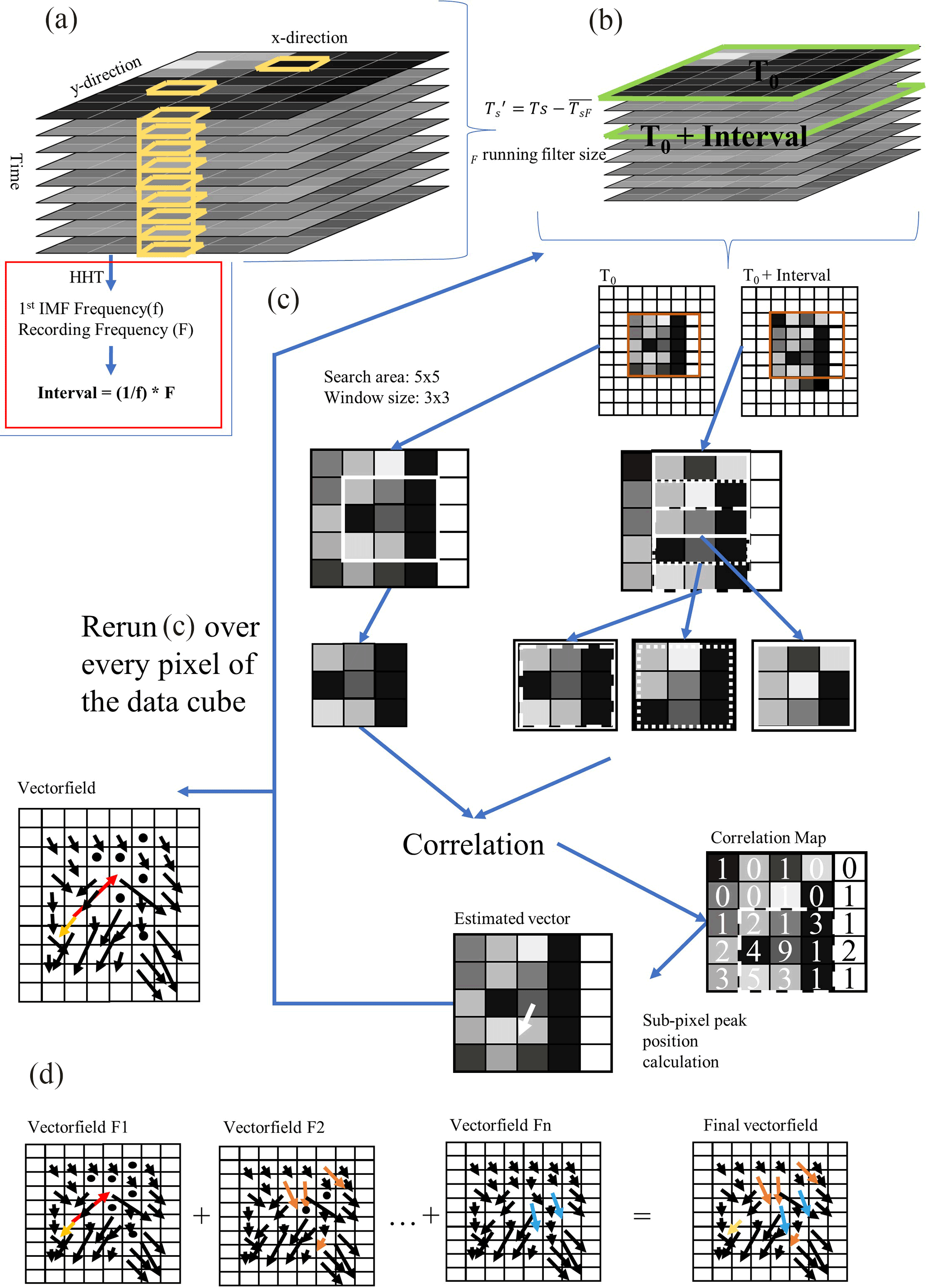
Figure 1Schematic of the A-TIV algorithm – (a) randomly selected stabilized brightness temperature pixels (marked orange) are used with HHT to find the highest-frequency signal component of the data set which defines the interval setting. (b) The perturbation calculation with different predefined running filter sizes (F) is done to provide the data for computation of the TIV core algorithm. From the perturbation data set two images with the time increment of the interval setting are extracted and passed to panel (c). (c) Core TIV algorithm with an example search area size of 5×5 pixels and a correlation window size of 3×3 pixels. Error vectors are adjusted using the standard deviation of the calculated vectors in the direct adjacent pixels. (d) The process from panel (c) is computed over all predefined filter sizes of panel (b) to calculate multiple vector fields that are available. Finally, all vector fields are merged using weighted averaging.
TIV previously used a correlation technique presented by Kaga et al. (1992) called the greyscale correlation technique, which uses simple pixel by pixel subtraction to obtain a correlation value (Inagaki et al., 2013). The A-TIV is usually calculated using the same technique with a correlation window size of 16×16 pixels and a search area size of 32×32 pixels. These settings were previously investigated as the most accurate (Schumacher et al., 2019).
Equation (1) shows calculation of perturbation for the data cube. is the resulting perturbation of 1 pixel, Ts is the measured brightness temperature of the pixel, and is the temporal mean of the pixel dependent on the filter size F (5, 10, 20, or 30 s). See Fig. 1b for context.
2.2 Adaptive thermal image velocimetry
The A-TIV algorithm is based on the same principle as the TIV algorithm with two new modifications (Fig. 1a red box and d), which allow an automatic adaptation of the algorithm to its input brightness temperature imagery and therefore the underlying environmental conditions. In previous investigations, the TIV algorithm showed a large sensitivity to the correlation time interval setting, delivering erroneous vectors when the setting was too short (see Sect. 3.2.1). Therefore, as a first development A-TIV takes advantage of the Hilbert–Huang transform (HHT), identifying the instantaneous frequencies of a given signal (Huang et al., 1998). In the case of A-TIV the first step of the HHT is to calculate the ensemble empirical mode decomposition (EEMD), which determines the intrinsic mode functions (IMFs) of the time series from 11 randomly selected pixels from the input thermal imagery (Wu and Huang, 2009). The second step is to calculate the Hilbert transform of the first IMF of each selected pixel, defining the highest instantaneous frequencies of the input thermal imagery. The average of the 11 calculated instantaneous frequencies prescribe the correlation time interval setting for the A-TIV algorithm. This allows us to change the interval setting based on variable experimental input data.
As a second development, A-TIV makes use of sequenced time filters in the perturbation calculation (see Eq. 1). The temporal filter size F in of the TIV algorithm is varied to cover multiple magnitudes of perturbations in the brightness temperature data set (see Fig. 2). When multiple perturbation filters are calculated on the stabilized brightness temperature data set, the resulting perturbation from the longest filter size F represents the largest scale of motion. One TIV sequence is calculated on each of these three-dimensional (3D) perturbation data cubes (x, y, time; see Fig. 1). All resulting velocity data cubes are subsequently assimilated from longest to shortest perturbation filter size using a weighted average with the filter size as weight (in this study 30, 20, 10, and 5 s or 6-fold, 4-fold, 2-fold, and 1-fold). This leads to a velocity field output which contains more information from the longest perturbation filter sizes. An increasing noise level of the camera is present with decreasing perturbation filter size. Therefore the weighted average is based on the perturbation filter size, which reduces the importance of the TIV output calculated from the smallest perturbation filter. This allows the A-TIV algorithm to include all velocity fields with reduced noise-associated disturbances. The calculation of the A-TIV also removes outliers of the output wind velocities by replacing values that are outside of 2 standard deviations with the mean value within a 3×3 window (see Fig. 1c).
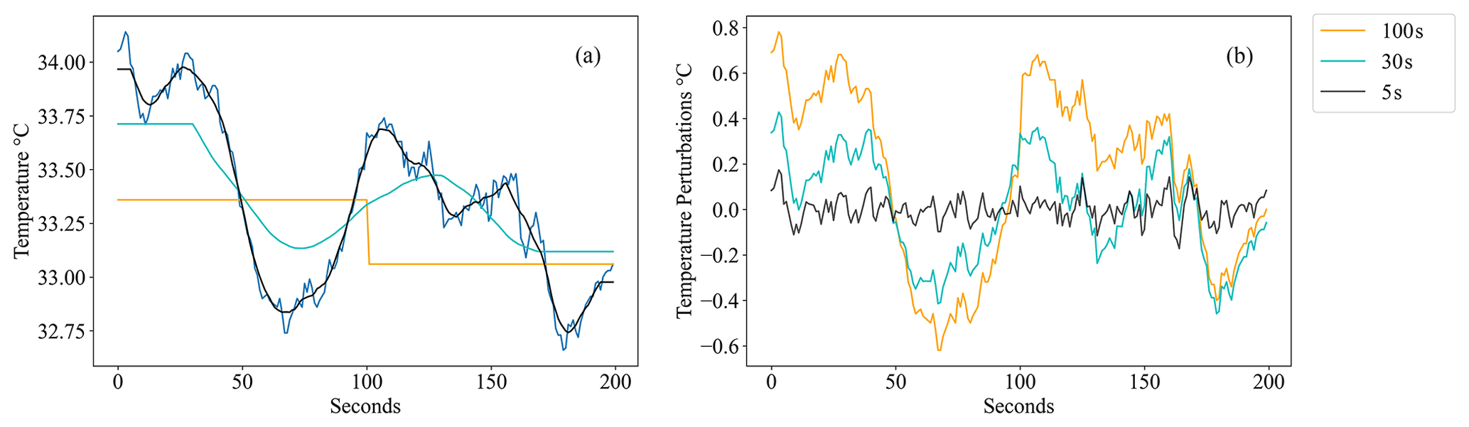
Figure 2Sample pixel: (a) temperature and (b) temperature perturbations – example showing impact of different running filter sizes to calculate the perturbations. (a) Temperature measurement from a sample pixel of the IR camera. Dark blue is the original temperature, and the smoothed lines are the running mean used for the perturbation calculation (see legend for the length). The corresponding perturbation scales are shown in panel (b). The mean of 100 s only allows large perturbation influences to be shown while the smaller perturbation window of 5 s accounts for small-scale changes.
According to Inagaki et al. (2013) perturbation filter sizes () from 1 to 30 s show a high correlation with near-surface measured wind velocity when calculating TIV. Therefore, the default setting is four different running filter sizes: 30, 20, 10, and 5 s.
2.3 Data
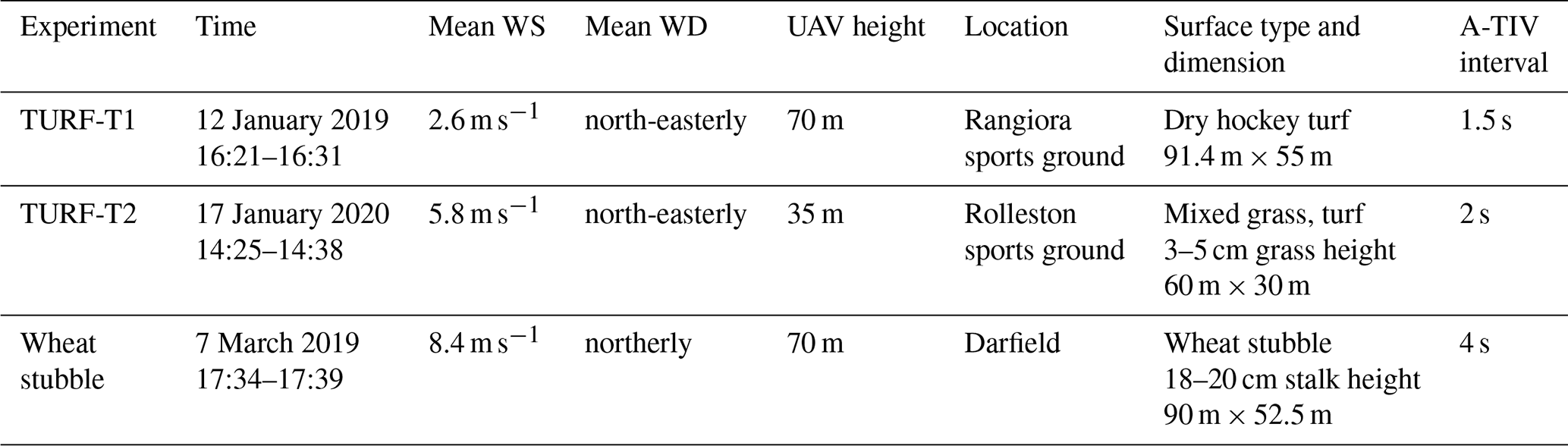
Three separate field experiments in the Canterbury region of New Zealand were carried out during the Australasian summer in January and March 2019 and in January 2020. The two time-sequential thermal infrared turbulence (TURF-T) experiments were equipped with sonic anemometers, fine-wire thermocouples, and an infrared camera on a UAV (Fig. 3). The first experiment TURF-T1 took place at a hockey turf field, and the second experiment TURF-T2 was held at a mixed surface with turf and grass. The third experiment included an infrared camera on a UAV acquiring footage over a dry wheat stubble field with a weather station in the proximity of 100 m collecting 1 min average wind speed. This third experiment was designed to test the algorithm when used over a higher vegetation canopy due to missing high-frequency measurements in a qualitative analysis. The weather station data were used to monitor the atmospheric conditions during the experiment day and put the A-TIV output from this experiment into context in the TURF-T1 experiment and TURF-T2 experiment.
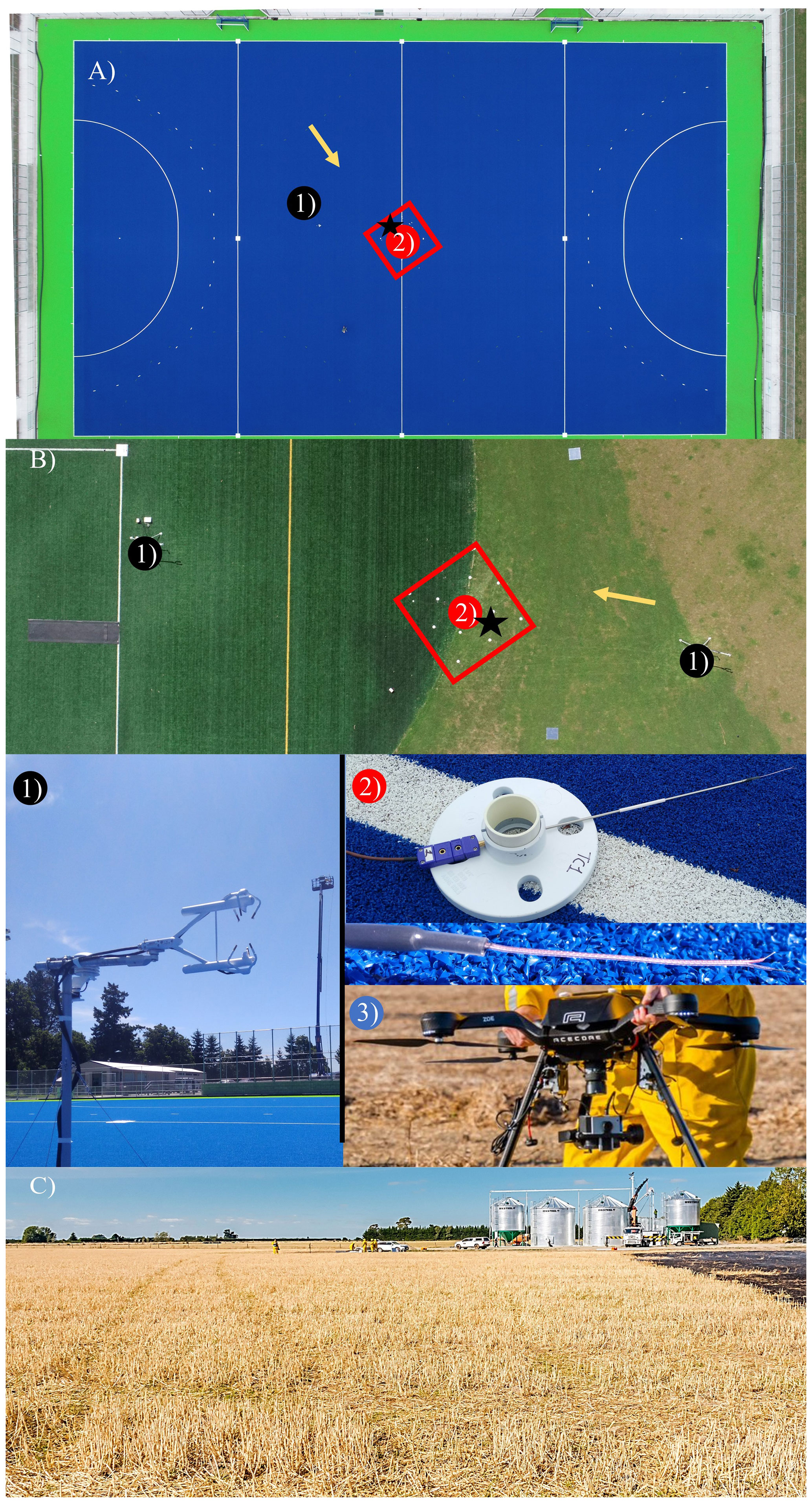
Figure 3Experiment sites and instrumentation – TURF-T1, TURF-T2, and wheat stubble experiment sites: (a) blue hockey turf, (b) green softball turf with surrounding grass, and (c) a harvested wheat field with stubble. In panels (a) and (b) the positions of sonic anemometer units (black dots, Image 1 – closeup below) and the thermocouple array (red square with red dots, Image 2 – closeup below) are marked. The black star shows the position of the base thermocouple upwind which was used for close surface wind velocity estimation (see Sect. 2.7). The mean wind direction is emphasized by a yellow arrow. Image 3 shows the used quadcopter with a three-axis inertial stabilizer and the Optris camera mounted.
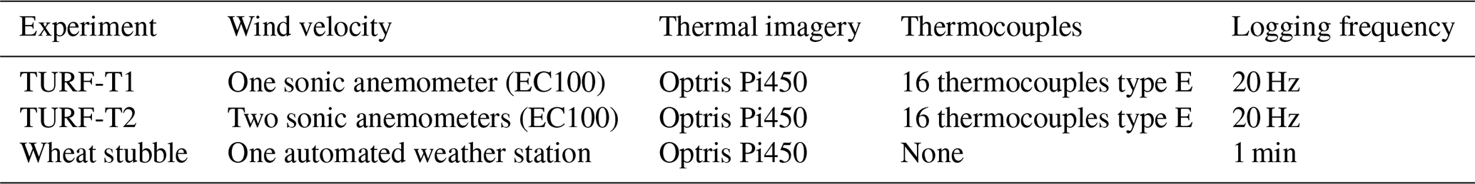
The wheat stubble experiment took place after the harvest of the crops when the individual stalk heights were cut to 18–20 cm and left standing upright in the field. Compared to the spikes of the wheat plant the stalks are a very stable part of the plant, and it was expected that even with higher wind gusts the stalks would not create any motion effects, also called “honamis”, interfering with the camera measurement (Finnigan, 2010). Table 1 provides a summary of the three experiments, and Table 2 provides a summary of the available instruments.
The surface types were picked in accordance with other field experiments, which suggest that the application of the TIV method is more suitable for dry and thermally responsive surfaces with a high thermal admittance (Inagaki et al., 2013; Christen et al., 2012). For the acquisition of the infrared video, the Optris PI 450, a lightweight, passively cooled camera with the capability to be attached and stabilized to a UAV using a three-axis dynamically responsive camera mount, was used (Fig. 3, Image 3). The camera measures a spectral range of 8 to 14 µm, in a resolution of 382×288 pixels, with a system accuracy of ±2 ∘C or 2 % of the measured temperature and a thermal sensitivity of 40 mK (Optris, 2020). Due to the passive cooling mechanism of the camera, its sensor is reset for 1 s in a frequency of 10 s. The camera lens used for all experiments is a wide-angle lens with a field of view of and a fixed aperture of . The acquisition frequency was set to 80 Hz, and the output file format is a radiometric video file.
In addition to the brightness temperature measurements, near-surface temperature and wind velocity measurements were made to compare the brightness temperature measurements and A-TIV wind speeds to the in situ meteorological measurements. TURF-T1 was equipped with one sonic anemometer, and TURF-T2 was equipped with two sonic anemometers, one in the grass field and one in the turf (Fig. 3). All anemometers were mounted at 1.5 m above ground level, sampled at 20 Hz, and placed in the field of view of the camera. Additionally, the TURF experiments were equipped with an array of fine-wire thermocouples (TC – 0.0254 mm bead diameter) mounted approximately 1.5 cm above the ground, measuring air temperature with a sampling speed at 20 Hz (Fig. 3, Image 2). The 12 sensors in the TC array were distributed in a square with three sensors per edge (eight sensors total) and four sensors aligned in the bisector of the square (Fig. 3), resulting in an interdistance of 1.5 m. This distribution ensured a proper lag correlation methodology to retrieve near-surface wind direction and wind velocity.
Meteorological conditions
Experiments were carried out when the Canterbury region was under the influence of stagnant anti-cyclonic (high-pressure) synoptic conditions with weak pressure gradients, resulting in near-surface wind speeds in the ranges of 2–5 m s−1. However, we expect differences in the characteristics of the boundary layer development (and hence the turbulence field) for each day. This will be due to the variation in cloud cover and the fact that the characteristics of the thermally generated flows (such as sea breezes) will be different for each day. The conditions on 7 March 2019 were additionally influenced by a low-pressure system to the southwest of New Zealand which caused higher wind speed ranges during this day. The TURF-T1 experiment day was characterized by cloudy conditions in the morning progressing to clear-sky conditions in the afternoon with an average temperature of 18.3 ∘C. This morning cloud cover did not interfere with the temperature during the TURF-T1 experiment. TURF-T2 was carried out with no cloud cover and an average air temperature of 20.6 ∘C. The wheat stubble experiment was carried out during a period with scattered high clouds and an average air temperature of 22.2 ∘C. For more detailed descriptions on the meteorological conditions during the experiments, see Table 1. For an overview of the used instrumentation please refer to Table 2.
2.4 Thermal imagery stabilization process
The unstable brightness temperature collected with a UAV-based system is stabilized using Blender, a 3D video animation software package (Cardona and Hartenstein, 2006; Ramos et al., 2011; Blender Online Community, 2019). A detailed description of the process is available in Schumacher et al. (2019), which can be summarized as follows: to read the collected brightness temperature video into Blender, the data are transferred to RGB colour value images. The Blender software is employed to track the camera movements using the manual camera tracking feature and the low-emissivity targets, which are displayed as cold spots in the imagery. Then the stabilization process was computed with a nearest-neighbour interpolation on the RGB colour images using low-emissivity targets in the field of view of the camera. Subsequently a random forest machine learning algorithm is trained on the unstable brightness temperature–colour value image pairs. The random forest algorithm in this case works as a colour value–temperature model. Finally, the stable temperature images were predicted from the stabilized colour images with the random forest algorithm. The effects of the stabilization for the TURF-T1 experiment are shown with the standard deviation of the images over time in Fig. 4. Before using the stabilized brightness temperature, it should be subsampled using averaging from the original acquisition frequency to a suitable noiseless frequency. For example, the TURF-T1 experiment data were subsampled from 80 to 2 Hz. The stabilized and subsampled video can be registered with a geographic coordinate system.

Figure 4Standard deviation over time for (a) unstable and (b) stabilized thermal imagery – impact of stabilization algorithm on the brightness temperature (Tb) standard deviation over time zoomed to a low-emissivity target of the TURF-T1 experiment. Panel (a) shows the unstable Tb standard deviation, and panel (b) shows the stabilized Tb standard deviation. Panel (c) shows RGB imagery with the blue turf and the low-emissivity target in the centre. The peaks of the standard deviation of panels (a) and (b) are shifted due to the working mechanism of the software stabilization. Any subsequent frame in the stabilization will be matched with the base frame (first frame), and the standard deviation peak is hence shifted towards this first frame.
2.5 Thermocouple analysis
The thermocouple (TC) array allowed us to estimate wind speed and wind direction very close to the surface, by estimating the lag cross-correlation on overlapping subsets (10 s) of TC time series data (20 Hz). The resulting 2 Hz TC-based advection wind velocity is calculated based on one TC measurement (base TC, black star in Fig. 3) lagged over 10 s and cross-correlated with all the surrounding TCs. The base TC was defined as one of the inner four TCs which was placed upwind of the other thermocouples. The TC-based advection wind speed was used in the accuracy assessment of the A-TIV algorithm.
The time lag and the distance of the TC with the highest correlation coefficient determined the wind velocity, and the position relative to the base TC determined the wind direction. Because of the overlapping 10 s windows in the time series, the resulting frequency of wind speed and wind directions measurements was 2 Hz. Due to maximal and minimal lag-correlation times, the minimal resolved wind velocity is limited to 0.25 m s−1.
To evaluate the brightness temperature data captured by the infrared camera with the TC derived air temperature in a first step, the same methodology was applied to a “virtual” array taken from the brightness temperature perturbations which were sub-sampled using mean sampling to a sampling rate of 20 Hz. The lag cross-correlation was calculated on this sampling rate, resulting in a 2 Hz wind direction and wind speed measurement identical to the physical array calculation. For the TURF-T1 experiment the centre of this virtual array was located about 9 m upwind from the centre of the physical TC array. The retrieved wind speed and wind direction were compared directly to the results from the physical array using a basic statistical t-test analysis and a histogram comparison. The same method was applied to the TURF-T2 experiment in which the physical array was distributed across both surfaces; hence, the virtual array was tested in three different positions: one in the grass field 9 m upwind of the physical array, one in the turf field 9 m downwind of the physical array, and one 1 m next to the physical array to resolve the same surface types for each TC.
2.6 A-TIV evaluation
The sonic anemometer data from the three experiments were used to calculate the mean wind speed over the experimental period to characterize the different meteorological conditions during the experiments (Table 1). The evaluation of the A-TIV-based thermal pattern velocity involved a statistical analysis with a comparison to the statistics of the TC and EC measurements. For the comparison, the A-TIV speeds were averaged over an area of 15 m × 15 m to ensure four homogeneous fields of turf (TURF-T1 and TURF-T2), grass (TURF-T2), and wheat stubble. In TURF-T2 the calculation of the A-TIV was separated for both surface types to be able to compare the results from the artificial to natural surface cover. The statistical analysis included an analysis of the probability density functions and a t-test comparison of the average of the thermal pattern speed from both TURF experiments to the TC measurements. Additionally, the algorithm performance from the wheat stubble experiment was analysed comparing the area-average A-TIV speed histograms of all experiments. For all comparisons histograms and probability density functions are presented rather than instantaneous cross-correlations because of the difference in measurement approaches meaning that A-TIV is resolving a near-surface spatial velocity whereas the sonic anemometers represent a point measurement of a spatial footprint, and the TC array measurements are representative of the immediate area where they are mounted. Therefore, the histograms and probability density functions provide a better overview of the similarities and differences than the time series from the measurements.
3.1 Stabilized brightness temperature evaluation
The TC array data were used to estimate wind speed and wind velocity approximately 1.5 cm above the ground using cross-correlation and the distance of the TCs (see Sect. 2.7). However, in a first analysis the brightness temperature (Tb) from the camera was used to create a virtual TC array to check if the data depict a similar measurement as the physical TC array. Figure 5 shows the histograms of the estimated wind speed and wind direction for TURF-T1 and TURF-T2 over grass and turf. In TURF-T1 the calculated wind speed and wind direction of the virtual TC array did not differ significantly from the physical TC array (p value >0.95). When the virtual TC array was placed in either the grass or the turf surface in TURF-T2 no similarity could be determined. However, when the virtual TC array was placed next to the physical array and the surface types of the virtual and the physical TCs matched a weak significant difference in wind speed, distribution was estimated (p value >0.9).
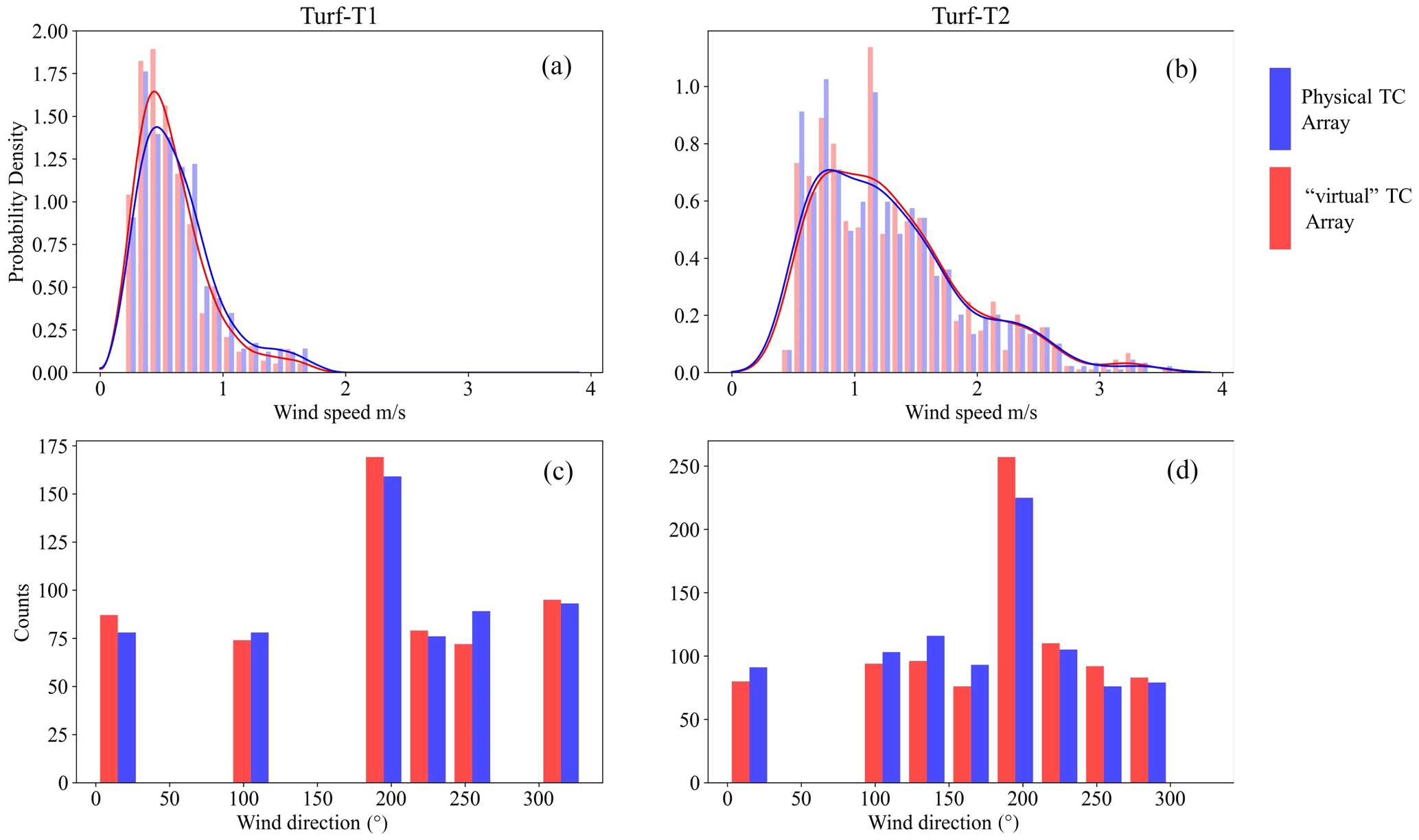
Figure 5TURF-T1 and TURF-T2 brightness temperature accuracy assessment – comparison of wind speed (a, b: metres per second) and wind direction (c, d: degrees) of the physical TC array (red) to the virtual TC array (blue) for TURF-T1 and TURF-T2. It is evident that the lag correlation using the virtual arrays depicts similar wind speed and direction as the physical TC array, which measures air temperature approximately 1.5 cm above the ground in both experiments.
3.2 A-TIV evaluation
3.2.1 TIV sensitivity to user input
The stabilization of UAV thermal imagery is the foundation for a successful TIV; however the A-TIV incorporates two steps to reduce error vectors (see Sect. 2.2) and create a more detailed output over non-artificial surface types. To show the advantages of the first step, an example frame of the TURF-T1 TIV is displayed with the correlation time interval setting informed by the HHT and compared to one with a user-defined correlation time interval setting (see Fig. 6). The TIV with the HHT as the correlation time interval setting mechanism removes error vectors and shows a larger spectrum of velocities. An error vector in Fig. 6 is defined as a vector which implies local, unrealistic measured A-TIV speeds (>6 m s−1), whereas during the experiment day the mean wind speed was measured at 2.6 m s−1.
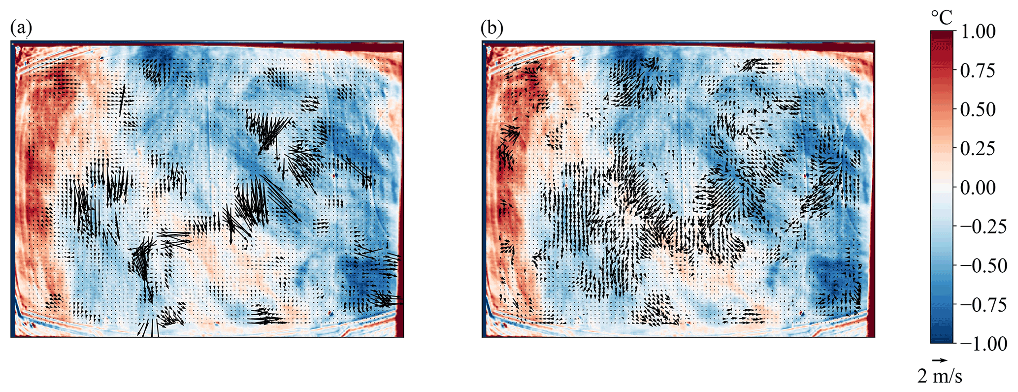
Figure 6Error vector removal due to correct correlation time interval setting – (a) a TURF-T1 TIV with a correlation time interval of 0.5 s. (b) The same TIV with an interval setting of 1.5 s, which was calculated using the HHT. The large error vectors mask the display of the small-scale vectors within panel (a).
The second step of A-TIV is the incorporation of the four perturbation calculations resulting in one TIV each, which are subsequently assimilated using a weighted average (see Sect. 2.2). Figure 7 shows an example frame of TURF-T1 with each of the four perturbation filters and the corresponding TIV with the HHT as the interval setting mechanism. The product A-TIV for this frame is the weighted average of these four TIVs.
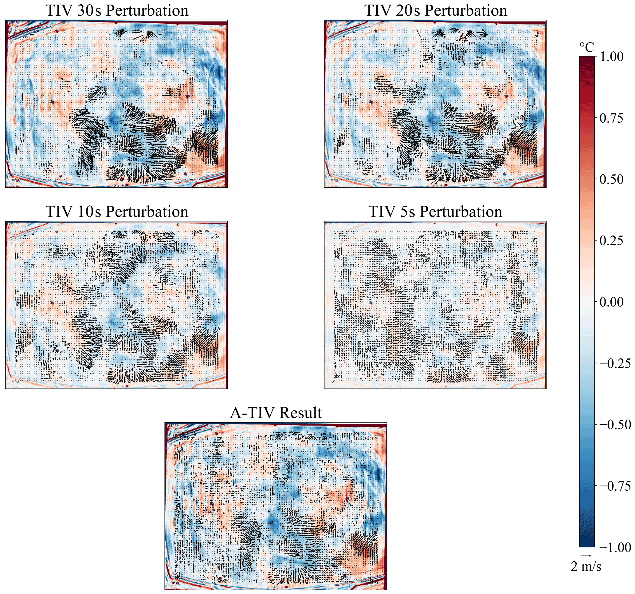
Figure 7TIV from four different temporal running filter sizes – extraction of TIV vectors from the four perturbation temporal running filter sizes 30–5 s. It is evident that with decreasing temporal running filter size more vectors are calculated.
3.2.2 Differences of A-TIV and TIV
A-TIV adds velocities to certain areas where the TIV does not estimate velocities (Fig. 6). The difference of A-TIV speed and TIV speed is displayed in Fig. 8. A positive difference indicates that the A-TIV speed is higher than the corresponding TIV speed of a certain perturbation filter size. Through the weighted averaging, the A-TIV gains with each new layer new information until the lowest perturbation filter adds the least amount of information due to its weight in the weighted average.
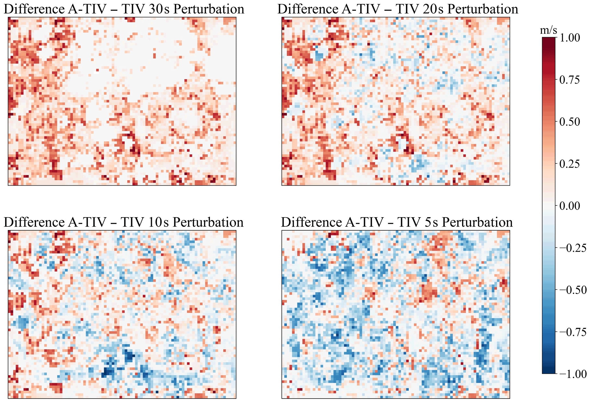
Figure 8A-TIV wind speed difference compared to the TIV result of TURF-T1 for an example frame – red indicates that the A-TIV result exhibits a higher speed than the corresponding TIV result. A positive difference means that all the other TIVs add velocity information to these pixels according to their weights (respectively meaning no velocity information is gained from this TIV pixel). A negative value means that velocity information is added from this pixel. A value close to zero means that the TIV of this pixel matches the A-TIV value. All velocity information gains and losses are changes in respect to the weight, which is defined by the perturbation filter time. A-TIV therefore gains information from different TIVs and creates an average measurement over various perturbation scales.
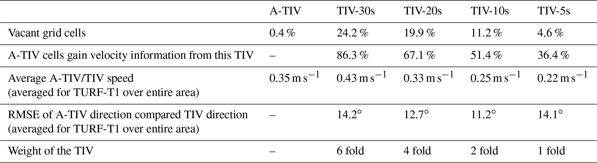
Table 3 shows the quantitative advantage of A-TIV over TIV. A-TIV provides fewer vacant grid cells compared to any TIV with a fixed perturbation filter size. Most of the velocities are added by the TIV with the highest perturbation filter size, whereas the other TIVs add less information to the final A-TIV product. The percentage given is the number of cells that add velocity information respective of the full number of available cells. Therefore, each TIV product could reach up to 100 % of added information.
Table 3Comparison of A-TIV with TIV – further qualitative information is also available in Appendix B.
3.2.3 Evaluation of A-TIV with wind velocity measurements
The A-TIV velocity fields for TURF-T1 were compared in two steps with the in situ available sensors, the sonic anemometer, and the lag-correlated thermocouple wind speeds. The first comparison covered the magnitude and timing of the perturbation scales of temperature and wind speed (Fig. 9). It showed that the A-TIV measurement matches the magnitudes of wind speed perturbation very well, when averaged over an area. There is also a clear timing difference of the perturbation peak occurrences between the A-TIV and the sonic anemometer data, which is expected due to the differences in measurement height and type.
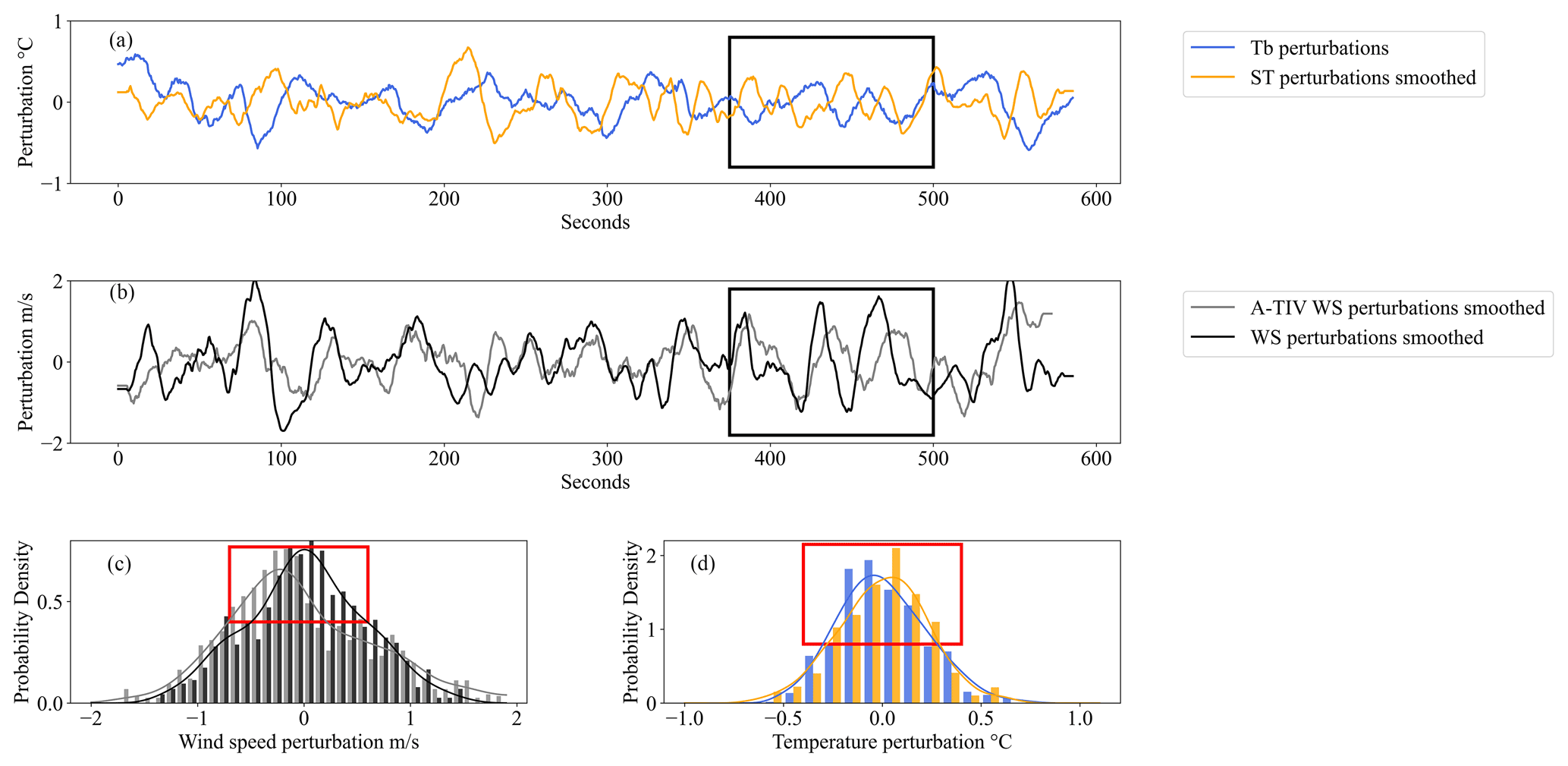
Figure 9TURF-T1 wind speed and temperature perturbations – TURF-T1 comparison of spatial average (15 m × 15 m) brightness temperature (Tb) perturbations (a, blue), with sonic temperature (ST) perturbations (a, orange), and the areal A-TIV wind speed perturbations (b, grey) with the measured wind speed perturbations from the eddy covariance/sonic anemometers (b, EC – black). Panels (a) and (b) show the timing of the measured temperature perturbations – see black square. The red rectangles in panels (b) and (c) show the differences in distribution of perturbations. The area of ∼ 15 m × 15 m for the calculation of the spatial average perturbations was picked slightly upwind of the sonic anemometer.
The second comparison also involved the turf and grass surface within the TURF-T2 experiment. This comparison revealed the different impacts of the surface types on the A-TIV measurement. In general, the TC wind speed distribution is shifted to higher wind speeds due to the limitations of the method allowing only wind speeds greater than 0.25 m s−1. Compared to the spatial TC wind speeds, A-TIV measures a similar wind speed distribution on the artificial surface type of TURF-T1, which confirms the results presented by Inagaki et al. (2013) (Fig. 10). With TURF-T2 a new mixed surface type was added, and A-TIV resolved generally higher wind speeds than the TURF-T1 experiment, which aligns the mean wind speed measured by the sonic anemometers (Table 1). The mean of the A-TIV speed distributions of TURF-T2 is 2.2 times higher than the TURF-T1 mean, which is a similar ratio to the average of the sonic anemometer mean wind speeds from both experiments (Table 4).
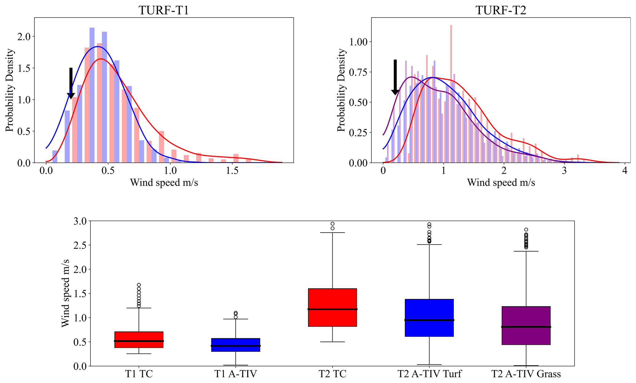
Figure 10TURF-T1 and TURF-T2 accuracy assessment with TC array – TURF-T1 and TURF-T2 wind speed histogram comparison. Blue histograms are A-TIV histograms of an area of ∼ 15 m × 15 m, the purple histogram shows the same area over grass, and red histograms are thermocouple wind speeds. The black arrows mark the cut-off point of the minimal resolvable wind speed of the lag-correlation method from the thermocouples. The boxplot on the bottom shows the differences in the median value of the displayed histograms. Across all surfaces the difference of the median is within ±0.4 m s−1.
Table 4Sonic anemometer mean wind speed compared to the A-TIV mean speed.
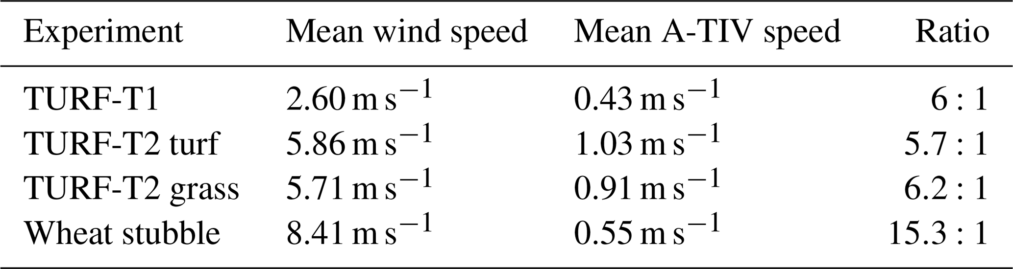
Figure 11 shows the relationship between A-TIV speeds compared to sonic anemometer wind speeds and TC wind speeds. The results are comparable with previously published relationships by Inagaki et al. (2013) over artificial surface types. Notable is that in the TURF-T2 experiment there is no significant relationship between the aerial average A-TIV speed and the wind speeds from the sonic anemometers.
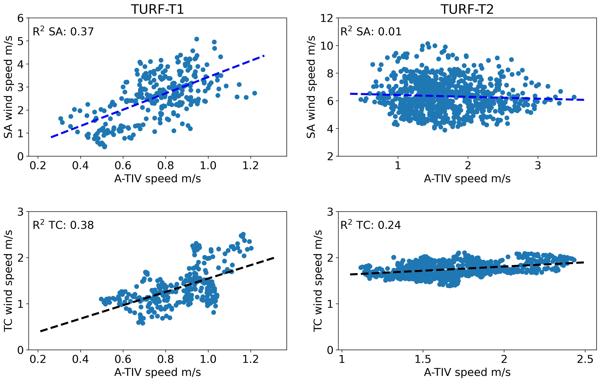
Figure 11A-TIV speed relationship with other measurement methods – TURF-T1 and TURF-T2 relationship of wind speeds measured by the sonic anemometer and the lag correlation of the TC array with the A-TIV speed. It is evident that TURF-T1 shows higher R2 values than TURF-T2. A weak relationship between the sonic anemometer and the A-TIV speed in TURF-T2 is evident.
3.2.4 Evaluation of A-TIV for higher roughness elements (wheat stubble)
The wheat stubble A-TIV was carried out to test the limitations of the A-TIV algorithm when a higher canopy (∼20 cm), which is not affected by wind-induced movements, is present. The effect of different perturbation temporal running filter size on the averaged vector field shows that the assimilation increases the number of higher wind speeds due to the shortest perturbation window (Fig. 12). However, through the weighted averaging in the A-TIV calculations the shortest perturbation window does not have a large impact on the combined final wind speeds (Fig. 12). Due to a fault in the high-frequency wind velocity measurements in the wheat stubble experiment, the A-TIV-based advection velocity measurement can not be compared to high-frequency in situ measurements and is therefore only of a qualitative nature. Nevertheless, when comparing the combined histograms from the A-TIV measurement of all experiments, we hypothesize that the canopy height is causing a decrease in measured A-TIV-based advection speed due to the influences of drag introduced by the canopy (Fig. 13). This is supported by the average wind speed ratios of the three experiments, which would also lead to a higher expected A-TIV velocity estimation (Table 4).
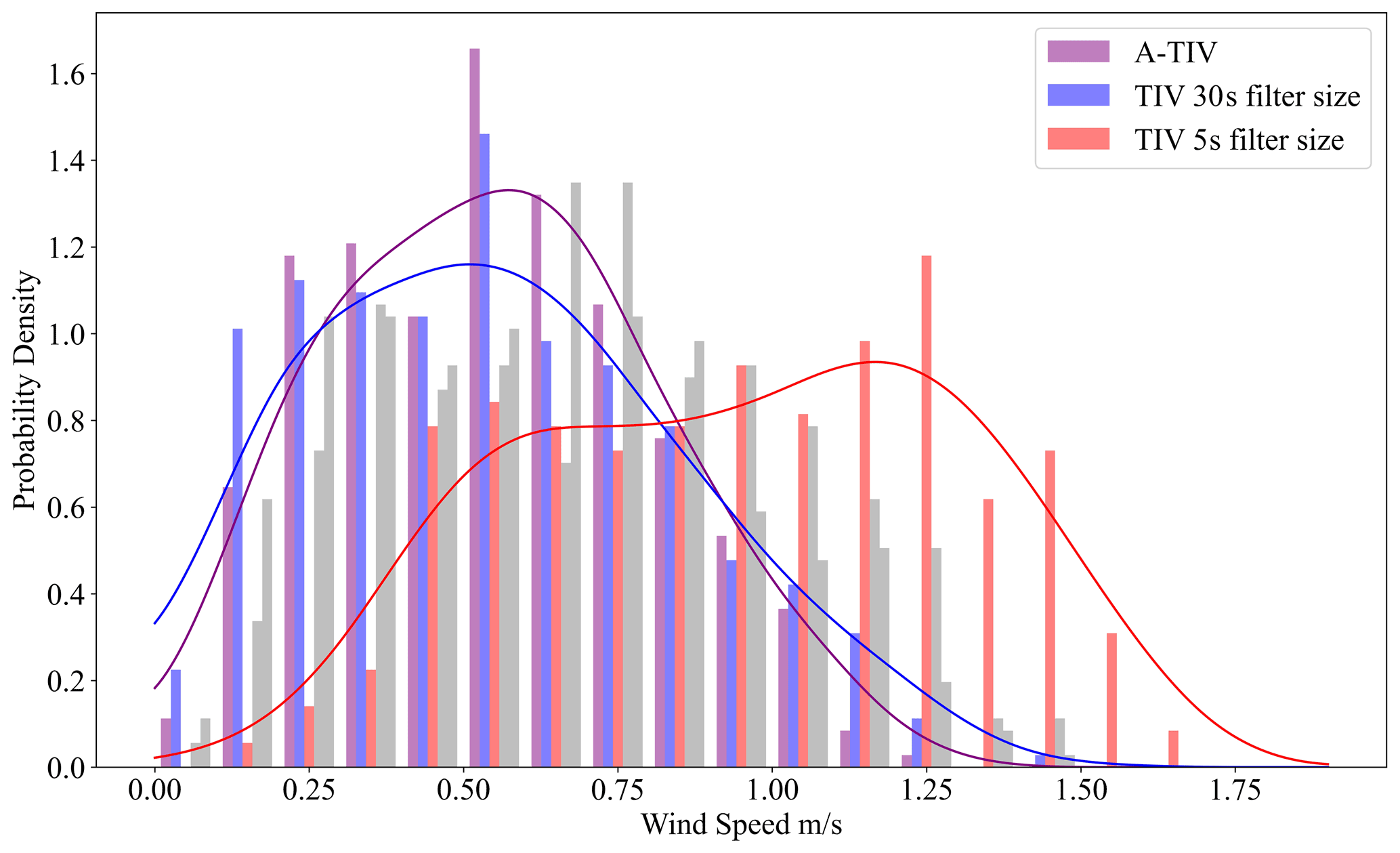
Figure 12Impact of the lowest and highest perturbation running filter size on the wheat stubble A-TIV result – the blue histogram is based on the 30 s perturbation window and the red histogram on the 5 s perturbation window. The combined final wind speed histogram is shown in purple. The perturbation temporal running filter sizes of 10 and 20 s are shown in grey.
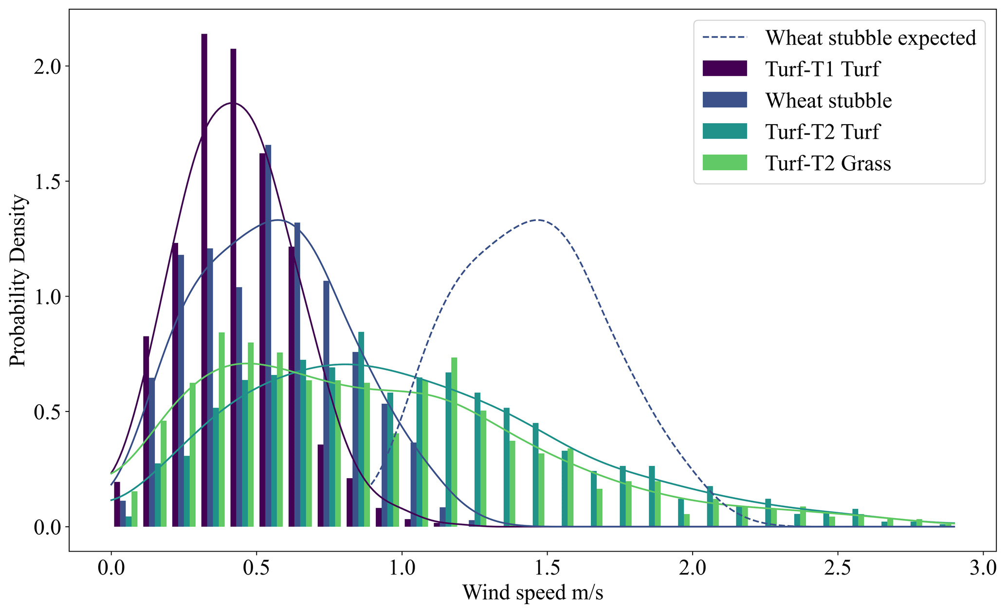
Figure 13A-TIV comparison of all experiments – probability density functions for the ∼ 15 m × 15 m average aerial wind speed from all experiments. It is evident that the wheat stubble experiment shows the lowest average wind speed histogram distribution whereas the mean wind speed was the highest during the experiment. The dashed line shows the expected probability density based on the ratio 6:1 calculated in Table 3. The decrease demonstrates the effect of the canopy.
A-TIV is a first effort to calculate a spatial atmospheric velocity measurement over natural surface types and make the algorithm available to a wider community in atmospheric science and near-target infrared remote sensing. Garai and Kleissl (2011) pointed out that movements of leaves or the movement of the canopy itself within the field of view of the sensor itself can influence the brightness temperature measurement. This can impact near-target infrared measurements also depending on the canopy height and the wind velocity (Garai and Kleissl, 2011; Finnigan, 2010). Due to the harvested wheat pasture, such effects are not expected for the wheat stubble experiment. However, the higher canopy of the wheat stubble has an additional insulation effect by absorbing thermal radiation. This radiation is emitting over longer periods of time, whereas short turf or grass emits the longwave thermal radiation faster. The effect of slower emittance over wheat stubble interferes with the brightness temperature perturbations, leading the A-TIV algorithm to estimate a low velocity distribution while higher mean wind velocity was measured (Fig. 13 and Table 1). Furthermore, the wheat stubble alters the wind profile above it more significantly compared to the smooth roughness elements of TURF-T1 and TURF-T2, which also affects the exchange of heat between the surface and the atmosphere.
Nonetheless, there are additional limitations involved when collecting brightness temperature from a UAV. To avoid noise and temperature spikes from external solar heating of the camera body, the Optris camera provides a resetting mechanism every 20 s for 1 s. During this period, the camera does not acquire images which then must be removed from the time sequence and possibly cause the timing delay of the calculated A-TIV velocity perturbations (Fig. 9). Furthermore, due to flight height restrictions of the UAV, a wide-angle lens was used to cover a larger area. This implies a distortion of the camera lens which has not been removed because the stabilization and the A-TIV algorithm involve cropping the edges of the images. An assessment of the pixel distortion showed that for the TURF-T1 experiment the maximal deviation from the calculated pixel size was 0.05 m. This error is within the error range of the TC array calculated wind speeds, which can be affected by the possible misplacement of the sensors on the ground. For TURF-T2 the distortion was further minimized by a lower flight height of the UAV, and hence a smaller field of view was covered (Table 1).
The final 2D velocity vector from A-TIV represents the interaction of atmospheric coherent structures with the surface. Structures can have a higher or lower velocity than suggested by the mean wind if the advection is not purely horizontal. Hence, A-TIV is not necessarily a direct measurement of the mean wind of the coherent structure causing the A-TIV velocity estimation. Furthermore, the estimations depend on the scale of the interaction in time and space. Larger structures than the defined correlation window size as well as small structures smaller than half of the correlation window size might not be resolved by the A-TIV algorithm.
An advantage of the A-TIV algorithm is that it provides a spatial measurement of wind velocities at the resolution of the camera sensor array. This is an advantage over traditional point-based measured velocities, which are limited to a spatial footprint dictated by the height of the sensor on a tower and the mean wind speed. The spatial near-surface velocity measurements through A-TIV can give valuable insight into the instantaneous turbulent eddy sizes, and future work can focus on evaluating the resolved turbulence spectra and comparing to spatial eddy covariance measurement campaigns. This is specifically advantageous when combining the two measurement approaches to further analyse the point measurements which depend on Taylor's hypothesis and are potentially prone to underestimating the turbulent spectrum in the inertial subrange (Taylor, 1938; Engelmann and Bernhofer, 2016; Cheng et al., 2017)
Furthermore, the A-TIV measurement may not reflect the same atmospheric turbulence compared to the sonic anemometer mounted at 1.5 m height. Previously Inagaki et al. (2013) applied a correction factor to the TIV measurements to compare them to sonic anemometers. This correction factor was not applied in this study because the measurement footprint of the sonic anemometer was larger, and the R2 values, specifically in TURF-T1, show similar correlation as determined by Inagaki et al. (2013).
The thermal interactions of structures with shorter timescales create a reduced amplitude in thermal perturbations measured by a sonic anemometer or measured by thermal imagery. Without a time–frequency decomposition on the signal, the sonic anemometer registers these as one time series integrating these scales and represented by a measured temperature or wind velocity. The TIV does not directly reflect this frequency composition and may reflect only certain frequencies due to the decomposition done in the calculation of the perturbation and the Hilbert–Huang transform. Higher frequencies and sensor noise are neglected in this way. To mitigate this indirect focus and limitation to certain frequencies, we introduced the A-TIV composition of multiple perturbation windows, which then allows us to reflect the reality better, which is a composition of superimposed multiple frequencies. In our case we decided to use 30, 20, 10, and 5 s because our thermal sensor's noise was only starting to interfere with the 5 s perturbation window. Therefore, we decided to use a weighted averaging system because it is expected that the noise level rises with the decrease in the temporal perturbation filter size. This is the case for any sensor used and is not limited to the thermal camera.
For any lower-quality camera systems that include more noise in the first detected frequency by the HHT, the second highest frequency may be picked. This may also be successfully used; however the A-TIV output may display more vacant grid cells.
A-TIV and TIV have only been tested in dry, warm environmental (approximately 20 ∘C) conditions with low latent heat flux present. Moisture, high roughness elements, and shading directly lower the fluctuations in the brightness temperature measurement caused by atmosphere–surface interactions. Further assessment is needed to test the range of environmental condition A-TIV can be applied to such as below-0 ∘C conditions. It is expected that this is mainly dependent on the amount of latent heat flux, the surface type, the canopy height, and the accuracy of the camera.
When comparing A-TIV measurements to eddy covariance measurements in TURF-T1 (Fig. 9), there is an indication for a coupling between the surface and the air temperature. But neither the wind speed perturbations nor the temperature perturbations show similar distributions. However, both measurements show similar magnitudes of perturbations. This emphasizes that the A-TIV captures cooling and heating patterns when the atmosphere is interacting with the surface. However, the histograms show that the distributions are not comparable, which is expected comparing a point measurement to a spatial approach. This means that the A-TIV reflects a spatial measurement whereas the other measurement methods are based on single-point measurements which depend on their mounting height and their footprint. The direct spatial measurement of A-TIV reflects the atmospheric situation directly adjacent to the surface and hence, when compared to point measurements further away from the surface, may not reflect the same conditions. The patch size of 15 m × 15 m to compare A-TIV to the eddy covariance measurements was chosen based on the size and the calculated footprint of the available upwind area (25 m × 20 m) of the sonic anemometers in the TURF experiments (see Appendix A on footprint calculation). To avoid corner effects, i.e. from obstacles, and to reflect the core of the calculated footprint, we decreased the size of the averaging area to 15 m × 15 m.
The assumption from Stull (1988) that meteorologists observe atmospheric conditions over longer periods of time (more than several hours) rather than creating short observations over a large region of interest does not reflect the strategy of A-TIV applications. According to Stull (1988) the long-term point measurements can be translated to their corresponding spatial measurements as a function of time. A-TIV is a new approach in the sense that the measurement type is directly spatial, and hence short-term observations can immediately reflect the spatial component of turbulence. Moreover, the new type of data that are retrieved need new spatiotemporal statistics and new analysis methods such as A-TIV for new insights into spatial turbulence.
Essentially the underestimation of A-TIV velocity measurements is a result of the difference in the measurement process between the TC lag correlation and the A-TIV. A-TIV will resolve only wind velocities when the coherent structures exhibit a temperature difference to the surface temperature. Therefore, A-TIV is fully based on the difference of spatial change in brightness temperature, whereas the lag-correlated TC wind speeds estimate motion based on air temperature changes measured in points and are not bound to the thermal properties of the surface. This means that the A-TIV algorithm will resolve surface–atmosphere interactions and motions of a certain scale very well. However very small-scale processes within the size of half of the correlation window size will not be resolved by the algorithm.
Specifically small spatial interactions with low velocities may not be reflected in the TIV estimations with a higher temporal running filter size (30 and 20 s in this paper). Therefore, the A-TIV includes velocities from lower temporal running filter sizes (10 and 5 s in this paper) and ensures that fewer vacant grid cells are present compared to any TIV. The display of very small velocities (<0.5 m s−1) is also not ideal due to the a high range of extracted velocities from the multiple TIVs neglecting the display of small velocities (Fig. 7).
It is evident that A-TIV speeds are related to the wind velocity measured by other measurement techniques (Fig. 9). However, when the wind speed increases, the relationship between the sonic anemometers and the A-TIV speeds is not as strong. This is likely due to the elongation of the thermal structures, which has been described before (Garai et al., 2013). Streaky surface structures are measured differently with the thermal camera compared to the sonic anemometer, which was mounted at 1.5 m height. More detailed investigations are needed to quantify the measurement differences and possibly the adjustments to the A-TIV algorithm to better resolve the surface layer turbulence.
The results from this research present an enhancement of the TIV algorithm: the adaptive thermal image velocimetry which enables it to derive spatial wind velocity measurements from thermal images at moderately high frequency (2 Hz) over artificial and non-artificial surfaces.
The key findings of this study are as follows.
-
High-frequency (>1 Hz) brightness temperature measurements over dry thermally responsive surfaces reflect similar atmospheric influences as near-surface (approximately 1.5 cm) temperature measurements (Fig. 5).
-
Brightness temperature measured with a UAV, when software image stabilization is applied, can be used to retrieve instantaneous spatial wind fields using A-TIV over artificial and non-artificial surface types (Fig. 10).
-
The TURF-T experiments showed that A-TIV can correctly resolve air temperature perturbation and wind speed perturbations and retrieve spatial velocity fields very close to the ground (approximately 1.5 cm) when compared to in situ lag-correlated thermocouple measurements (Figs. 9 and 10).
-
The wheat stubble experiment showed the impact of the canopy height on the A-TIV wind speed distribution. Further investigation is needed to evaluate the impact of the canopy height on the algorithm settings (Fig. 13).
The key limitations for a successful retrieval of higher-frequency A-TIV velocities are the camera's noise levels and the spatial field of view of the camera. This means that small infrared cameras carried from UAVs deliver high acquisition rates (Optris Pi 450: 80 Hz). However due to the camera noise present at this frequency, they need average sub-sampling to lower frequencies to enable analysis on the brightness temperature imagery. This is in direct connection with the camera's distance to the target surface where the acquired temperature differences become less due to the physical property of infrared light carrying less energy than visible light. This creates a feedback with the electrical noise of the camera. Therefore, depending on the acquisition situation, we suggest a careful assessment of all environmental parameters to retrieve optimal results. In similar conditions as presented in this study, a sub-sampling averaging to <3 Hz is recommended.
The potential of thermal cameras in remote sensing of micro-meteorology is large, and the A-TIV algorithm can be seen as a new opportunity for advanced analysis methods of spatial velocity field measurements. Further investigation will be needed to optimize the algorithm's performance and usability, especially over new surface types, to make it available for a larger community of remote sensing specialists and atmospheric scientists.
The footprints used for comparison of the sonic anemometer measurements with the A-TIV algorithm were calculated using the Urban Multi-scale Environmental Predictor (UMEP) (Lindberg et al., 2018) with input data from Land Information New Zealand and the measured variables. The footprint model used in the calculation was set to Kormann and Meixner (2001). For TURF-T1 and TURF-T2 the averaging area (15 m×15 m) was picked within the field of view of the infrared camera and covered ∼60 % of the cumulative source area (see Fig. A1 for an example from TURF-T1).
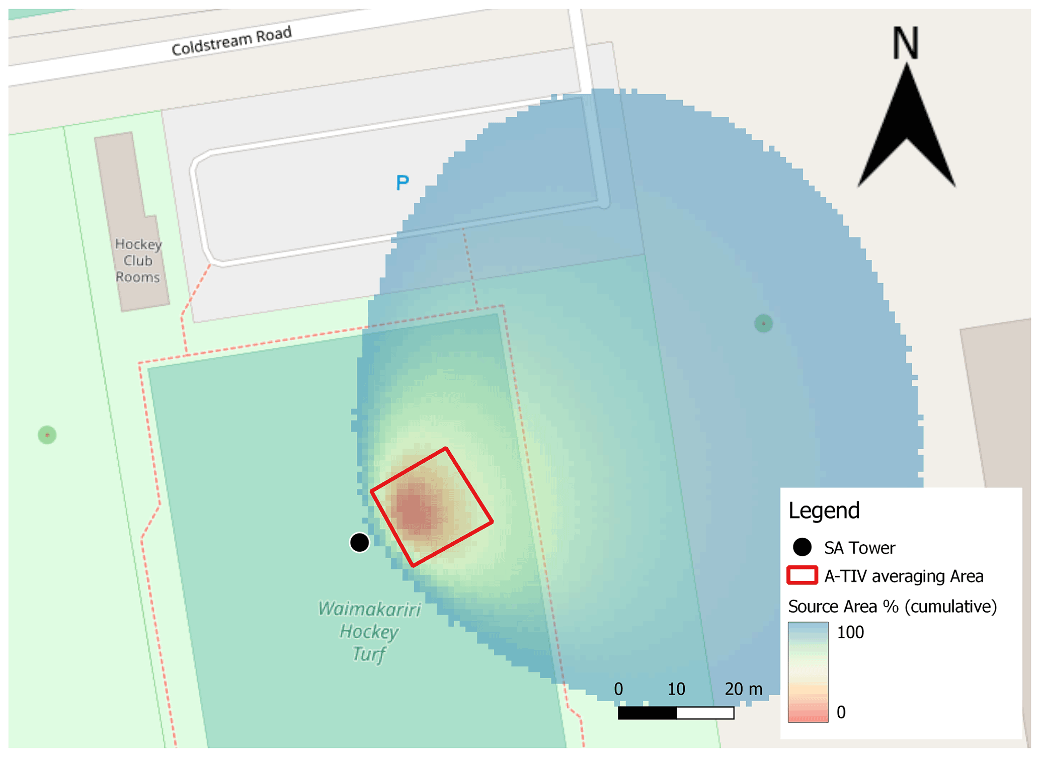
Figure A1Footprint calculated from the TURF-T1 experiment – background Image: © OpenStreetMap contributors 2022. Distributed under the Open Data Commons Open Database License (ODbL) v1.0.
The qualitative comparison of A-TIV wind speed and wind direction with TIV wind speed and wind direction is shown in Figs. B1 and B2. While the TIV wind speed depends mainly on the perturbation filter sizes, the A-TIV reflects the weighted mean of all calculated TIVs and removes outliers that may depend on camera noise or short temporal thermal disturbances within the measured thermal perturbation. On the other hand the measured wind direction signal of A-TIV compared to TIV is very similar. This shows that both methods reflect directions of moving thermal patterns correctly.

Figure B1Qualitative comparison of A-TIV wind speeds to TIV wind speeds of TURF-T1. The speeds are averaged over the entire area of the turf field. TIV speeds from the perturbation filters 10 and 20 s would be located between the 5 and the 30 s wind speeds and are not shown in this plot.
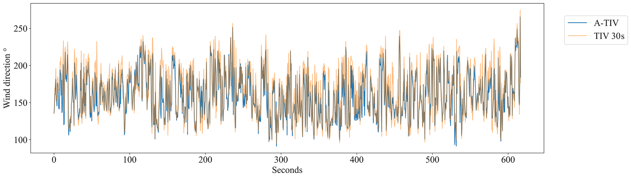
Figure B2Qualitative comparison of A-TIV wind directions to TIV wind speeds of TURF-T1. The directions are averaged over the entire area of the turf field. TIV directions and A-TIV directions are very similar; hence this plot shows only the 30 s TIV directions and the A-TIV directions. For a quantitative comparison please refer to Table 3.
The open-source code to use TIV and A-TIV is available on GitHub (https://doi.org/10.5281/zenodo.4741550, Schumacher, 2021).
The data from the presented experiments at are published at https://doi.org/10.5281/zenodo.4741550 (Schumacher, 2021) and https://doi.org/10.5281/zenodo.6961047 (Schumacher and Katurji, 2022).
MZ was involved in the conceptual framework of the experiments and the infrared data acquisition and analysis. BA supervised the software development which was carried out by BS. JZ was involved in the conceptualization of the stabilization. PZR and MK are responsible for the funding acquisition. BS and MK designed and conducted the experiments and analysed the data. BS prepared the manuscript with contributions from all co-authors.
The contact author has declared that none of the authors has any competing interests.
Publisher’s note: Copernicus Publications remains neutral with regard to jurisdictional claims in published maps and institutional affiliations.
This work was carried out under the framework of the research programme “The invisible realm of atmospheric coherent turbulent structures: Resolving their dynamics and interaction with the Earth's surface”, which was funded by the Royal Society of New Zealand. We want to express special thanks to Justin Harrison, Paul Bealing, and Nicholas Key, who helped with the TURF experiments and the UAV operations. A special thanks to the Scion field crew for supporting the wheat stubble experiment: David Glogoski, Max Novoselov, Richard Parker, Brooke O’Connor, Emma Percy, Ilze Pretorius, Veronica Clifford, Jessica Kerr, Kate Melnik, and Grant Pearce.
This research has been supported by the Royal Society Te Apārangi (grant no. RDF-UOC1701).
This paper was edited by Marcos Portabella and reviewed by two anonymous referees.
Adrian, R., Meinhart, C., and Tomkins, C.: Vortex organization in the outer region of the turbulent boundary layer, J. Fluid Mech., 422, 1–54, https://doi.org/10.1017/S0022112000001580, 2000. a
Alekseychik, P., Katul, G., Korpela, I., and Launiainen, S.: Eddies in motion: visualizing boundary-layer turbulence above an open boreal peatland using UAS thermal videos, Atmos. Meas. Tech., 14, 3501–3521, https://doi.org/10.5194/amt-14-3501-2021, 2021. a
Barthlott, C., Drobinski, P., Fesquet, C., Dubos, T., and Pietras, C.: Long-term study of coherent structures in the atmospheric surface layer, Bound.-Lay. Meteorol., 125, 1–24, https://doi.org/10.1007/s10546-007-9190-9, 2007. a
Bastiaanssen, W., Menenti, M., Feddes, R., and Holtslag, A.: A remote sensing surface energy balance algorithm for land (SEBAL). 1. Formulation, J. Hydrol., 212–213, 198–212, https://doi.org/10.1016/s0022-1694(98)00253-4, 1998. a
Blender Online Community: Blender – a 3D modelling and rendering package, Blender Foundation, Blender Institute, Amsterdam, http://www.blender.org (last access: 24 June 2022), 2019. a
Brenner, C., Thiem, C. E., Wizemann, H.-D., Bernhardt, M., and Schulz, K.: Estimating spatially distributed turbulent heat fluxes from high-resolution thermal imagery acquired with a UAV system, Int. J. Remote Sens., 38, 3003–3026, https://doi.org/10.1080/01431161.2017.1280202, 2017. a
Brenner, C., Zeeman, M., Bernhardt, M., and Schulz, K.: Estimation of evapotranspiration of temperate grassland based on high-resolution thermal and visible range imagery from unmanned aerial systems, Int. J. Remote Sens., 39, 5141–5174, https://doi.org/10.1080/01431161.2018.1471550, 2018. a
Cardona, A. M. and Hartenstein, V.: Three-dimensional skin reconstruction by vector sequence alignment and morphing, Blender Conference, 2006, Waag, Amsterdam, the Netherlands, 20–22 October 2006. a
Cheng, Y., Sayde, C., Li, Q., Basara, J., Selker, J., Tanner, E., and Gentine, P.: Failure of Taylor's hypothesis in the atmospheric surface layer and its correction for eddy-covariance measurements, Geophys. Res. Lett., 44, 4287–4295, https://doi.org/10.1002/2017GL073499, 2017. a
Christen, A., Meier, F., and Scherer, D.: High-frequency fluctuations of surface temperatures in an urban environment, Theor. Appl. Climatol., 108, 301–324, https://doi.org/10.1007/s00704-011-0521-x, 2012. a, b, c
Engelmann, C. and Bernhofer, C.: Exploring Eddy-Covariance Measurements Using a Spatial Approach: The Eddy Matrix, Bound.-Lay. Meteorol., 161, 1–17, https://doi.org/10.1007/s10546-016-0161-x, 2016. a
Finnigan, J. J.: Waving plants and turbulent eddies, J. Fluid Mech., 652, 1–4, https://doi.org/10.1017/s0022112010001746, 2010. a, b
Garai, A. and Kleissl, J.: Air and Surface Temperature Coupling in the Convective Atmospheric Boundary Layer, J. Atmos. Sci., 68, 2945–2954, https://doi.org/10.1175/JAS-D-11-057.1, 2011. a, b, c, d
Garai, A., Pardyjak, E., Steeneveld, G.-J., and Kleissl, J.: Surface Temperature and Surface-Layer Turbulence in a Convective Boundary Layer, Bound.-Lay. Meteorol., 148, 51–72, https://doi.org/10.1007/s10546-013-9803-4, 2013. a, b, c
Giordano, C., Vernin, J., Vázquez Ramió, H., Muñoz-Tuñón, C., Varela, A. M., and Trinquet, H.: Atmospheric and seeing forecast: WRF model validation with in situ measurements at ORM, Mon. Not. R. Astron. Soc., 430, 3102–3111, https://doi.org/10.1093/mnras/stt117, 2013. a
Hommema, S. and Adrian, R.: Packet structure of surface eddies in the atmospheric boundary layer, Bound.-Lay. Meteorol., 106, 147–170, https://doi.org/10.1023/A:1020868132429, 2003. a, b
Hoyano, A., Asano, K., and Kanamaru, T.: Analysis of the sensible heat flux from the exterior surface of buildings using time sequential thermography, Atmos. Environ., 33, 3941–3951, https://doi.org/10.1016/S1352-2310(99)00136-3, 1999. a, b
Huang, N. E., Shen, Z., Long, S. R., Wu, M. C., Shih, H. H., Zheng, Q., Yen, N.-C., Tung, C. C., and Liu, H. H.: The empirical mode decomposition and the Hilbert spectrum for nonlinear and non-stationary time series analysis, P. Roy. Soc. A-Math. Phy., 454, 903–995, https://doi.org/10.1098/rspa.1998.0193, 1998. a
Inagaki, A.: Application of the Thermal Image Velocimetry to Measure and Visualize Spatial Distribution of Near Surface Wind, Journal of Japan Society of Civil Engineers, 29, 186–195, https://doi.org/10.3178/jjshwr.29.186, 2016. a
Inagaki, A. and Kanda, M.: Organized Structure of Active Turbulence Over an Array of Cubes within the Logarithmic Layer of Atmospheric Flow, Bound.-Lay. Meteorol., 135, 209–228, https://doi.org/10.1007/s10546-010-9477-0, 2010. a
Inagaki, A., Kanda, M., Onomura, S., and Kumemura, H.: Thermal Image Velocimetry, Bound.-Lay. Meteorol., 149, 1–18, https://doi.org/10.1007/s10546-013-9832-z, 2013. a, b, c, d, e, f, g, h, i, j, k
Kaga, A., Inoue, Y., and Yamaguchi, K.: Application of a Fast Algorithm for Pattern Tracking on Airflow Measurements, in: Flow Visualization VI, edited by: Tanida, Y. and Miyashiro, H., Springer, Berlin, Heidelberg, https://doi.org/10.1007/978-3-642-84824-7_153, 1992. a
Katul, G., Schieldge, J., Hsieh, C., and Vidakovic, B.: Skin temperature perturbations induced by surface layer turbulence above a grass surface, Water Resour. Res., 34, 1265–1274, https://doi.org/10.1029/98WR00293, 1998. a
Kormann, R. and Meixner, F. X.: An Analytical Footprint Model For Non-Neutral Stratification, Bound.-Lay. Meteorol., 99, 207–224, https://doi.org/10.1023/a:1018991015119, 2001. a
Lindberg, F., Grimmond, C., Gabey, A., Huang, B., Kent, C. W., Sun, T., Theeuwes, N. E., Järvi, L., Ward, H. C., Capel-Timms, I., Chang, Y., Jonsson, P., Krave, N., Liu, D., Meyer, D., Olofson, K. F. G., Tan, J., Wästberg, D., Xue, L., and Zhang, Z.: Urban Multi-scale Environmental Predictor (UMEP): An integrated tool for city-based climate services, Environ. Modell. Softw., 99, 70–87, https://doi.org/10.1016/j.envsoft.2017.09.020, 2018. a
Litt, M., Sicart, J.-E., and Helgason, W.: A study of turbulent fluxes and their measurement errors for different wind regimes over the tropical Zongo Glacier (16∘ S) during the dry season, Atmos. Meas. Tech., 8, 3229–3250, https://doi.org/10.5194/amt-8-3229-2015, 2015. a
Lotfy, E. R., Abbas, A. A., Zaki, S. A., and Harun, Z.: Characteristics of Turbulent Coherent Structures in Atmospheric Flow Under Different Shear–Buoyancy Conditions, Bound.-Lay. Meteorol., 173, 115–141, https://doi.org/10.1007/s10546-019-00459-y, 2019. a
Morrison, T. J., Calaf, M., Fernando, H. J. S., Price, T. A., and Pardyjak, E. R.: A methodology for computing spatially and temporally varying surface sensible heat flux from thermal imagery, Q. J. Roy. Meteor. Soc., 143, 2616–2624, https://doi.org/10.1002/qj.3112, 2017. a, b
Optris: Optris PI450i Data Sheet, https://www.optris.de/infrarotkamera-optris-pi400i-pi450i?file=tl_files/pdf/Downloads/Infrarotkamera/Datenblatt optris PI 450i.pdf (last access: 19 October 2021), 2020. a
Paw U, K. T., Brunet, Y., Collineau, S., Shaw, R. H., Maitani, T., Qiu, J., and Hipps, L.: On coherent structures in turbulence above and within agricultural plant canopies, Agr. Forest Meteorol., 61, 55–68, https://doi.org/10.1016/0168-1923(92)90025-y, 1992. a
Pozníková, G., Fischer, M., van Kesteren, B., Orság, M., Hlavinka, P., Žalud, Z., and Trnka, M.: Quantifying turbulent energy fluxes and evapotranspiration in agricultural field conditions: A comparison of micrometeorological methods, Agr. Water Manage., 209, 249–263, https://doi.org/10.1016/j.agwat.2018.07.041, 2018. a
Ramos, T. C. P., Freymüller-Haapalainen, E., and Schenkman, S.: Three-dimensional reconstruction of Trypanosoma cruzi epimastigotes and organelle distribution along the cell division cycle, Cytometry, 79A, 538–544, https://doi.org/10.1002/cyto.a.21077, 2011. a
Sagaut, P. and Deck, S.: Large eddy simulation for aerodynamics: status and perspectives, Philos. T. Roy. Soc. A, 367, 2849–2860, https://doi.org/10.1098/rsta.2008.0269, 2009. a
Schumacher, B.: Adaptive Thermal Image Velocimetry, Version v0.1, Zenodo [code], https://doi.org/10.5281/zenodo.4741550, 2021. a, b
Schumacher, B. and Katurji, M.: Time seqUential theRmal inFrared – Turbulence campaign 1 – TURF-T1 Experiment data, Version TURF-T1, Zenodo [data set], https://doi.org/10.5281/zenodo.6961047, 2022. a
Schumacher, B., Katurji, M., Zhang, J., Stiperski, I., and Dunker, C.: Evolution of micrometeorological observations Instantaneous spatial and temporal surface wind velocity from thermal image processing, Geocomputation Conference 2019, University of Auckland, https://doi.org/10.17608/k6.auckland.9869942.v1, 2019. a, b, c, d
Simpson, J. E., Holman, F., Nieto, H., Voelksch, I., Mauder, M., Klatt, J., Fiener, P., and Kaplan, J. O.: High Spatial and Temporal Resolution Energy Flux Mapping of Different Land Covers Using an Off-the-Shelf Unmanned Aerial System, Remote Sensing, 13, 1286, https://doi.org/10.3390/rs13071286, 2021. a
Stull, R.: An Introduction to Boundary Layer Meteorology, Springer Science & Business Media, ISBN: 978-94-009-3027-8, 1988. a, b, c
Taylor, G.: The spectrum of turbulence, P. Roy. Soc. A-Math. Phy., 164, 0476–0490, https://doi.org/10.1098/rspa.1938.0032, 1938. a
Waters, R.: Surface Energy Balance Algorithms for Land – Idaho Implementation, Waters Consulting and University of Idaho and WaterWatch Inc., Nelson British Columbia, http://www.posmet.ufv.br/wp-content/uploads/2016/09/MET-479-Waters-et-al-SEBAL.pdf (last access: 24 June 2022), 2002. a
Wu, Z. and Huang, N. E.: ENSEMBLE EMPIRICAL MODE DECOMPOSITION: A NOISE-ASSISTED DATA ANALYSIS METHOD, Advances in Adaptive Data Analysis, 01, 1–41, https://doi.org/10.1142/s1793536909000047, 2009. a
- Abstract
- Introduction
- Methodology
- Results
- Discussion
- Conclusions
- Appendix A: Footprint calculation
- Appendix B: A-TIV – TIV wind speed and wind direction comparison
- Code availability
- Data availability
- Author contributions
- Competing interests
- Disclaimer
- Acknowledgements
- Financial support
- Review statement
- References