Meteor radar vertical wind observation biases and mathematical debiasing strategies including the 3DVAR+DIV algorithm

Meteor radars have become widely used instruments to study atmospheric dynamics, particularly in the 70 to 110 km altitude region. These systems have been proven to provide reliable and continuous measurements of horizontal winds in the mesosphere and lower thermosphere. Recently, there have been many attempts to utilize specular and/or transverse scatter meteor measurements to estimate vertical winds and vertical wind variability. In this study we investigate potential biases in vertical wind estimation that are intrinsic to the meteor radar observation geometry and scattering mechanism, and we introduce a mathematical debiasing process to mitigate them. This process makes use of a spatiotemporal Laplace filter, which is based on a generalized Tikhonov regularization. Vertical winds obtained from this retrieval algorithm are compared to UA-ICON model data. This comparison reveals good agreement in the statistical moments of the vertical velocity distributions. Furthermore, we present the first observational indications of a forward scatter wind bias. It appears to be caused by the scattering center's apparent motion along the meteor trajectory when the meteoric plasma column is drifted by the wind. The hypothesis is tested by a radiant mapping of two meteor showers. Finally, we introduce a new retrieval algorithm providing a physically and mathematically sound solution to derive vertical winds and wind variability from multistatic meteor radar networks such as the Nordic Meteor Radar Cluster (NORDIC) and the Chilean Observation Network De meteOr Radars (CONDOR). The new retrieval is called 3DVAR+DIV and includes additional diagnostics such as the horizontal divergence and relative vorticity to ensure a physically consistent solution for all 3D winds in spatially resolved domains. Based on this new algorithm we obtained vertical velocities in the range of w = ± 1–2 m s⁻¹ for most of the analyzed data during 2 years of collection, which is consistent with the values reported from general circulation models (GCMs) for this timescale and spatial resolution.

1 Introduction

Vertical wind in the mesosphere–lower thermosphere (MLT) is a key parameter because it is directly related to the vertical transport of momentum, energy, and constituents that drive the global meridional circulation, which is related to almost all dynamical processes in the global atmosphere (e.g., Smith et al., 2010; Qian et al., 2017; Guo and Liu, 2021). However, measuring vertical wind is one of the most challenging remote sensing tasks. The main reason is that the magnitude of long-term mean vertical wind is very small, often beyond the accuracy achievable with any instruments, while instantaneous, or short-duration, vertical wind can be large but requires measurements at high temporal and spatial resolutions. Models predict vertical motions on seasonal timescales at their typical horizontal grid resolution of about 100–200 km, which is on the order of 0.1cm s⁻¹ to a few meters per second, e.g., in the Kühlungsborn Mechanistic Circulation Model (KMCM) and the Whole Atmosphere Community Circulation Model (WACCM) (Holton, 1983; Becker, 2012; Smith, 2012). At higher solutions, the models are able to resolve smaller-scale gravity waves and produce larger vertical winds. In Liu et al. (2014), the high-resolution WACCM at 0.25^∘ horizontal resolution produced vertical wind of 7–8 m s⁻¹ in the lower thermosphere above a tropical cyclone. In a more recent study using the High-Altitude Mechanistic Circulation Model (HIAMCM) with a horizontal resolution of about 55 km, vertical wind speeds up to 3 m s⁻¹ were reported at an altitude of about 80 km (Becker and Vadas, 2018). High-resolution observations such as those made with a sodium lidar also measured vertical wind, showing that tidal perturbation in vertical wind can reach tens of meters per second (Yuan et al., 2014). On the other hand, models and observations also indicate that the horizontal wind magnitudes at the MLT are typically 1 to 2 orders of magnitude larger (Miyoshi et al., 2017; McCormack et al., 2017; Borchert et al., 2019; Hocking et al., 1997; Batista et al., 2004; Hoffmann et al., 2007; Jacobi et al., 2009; Wilhelm et al., 2019; Stober et al., 2020). This large difference in the magnitudes between the horizontal and vertical wind component poses an additional challenge to observational methods, measurement analysis, and parameter estimation for vertical wind due to the requirement of clear separation between vertical and horizontal components.

During the past decades there have been many attempts to measure vertical wind velocities using high-power, large-aperture radars such as EISCAT (Fritts et al., 1990; Hoppe and Fritts, 1995a, b). These EISCAT observations, with a temporal resolution of seconds, showed vertical velocities up to ± 10 m s⁻¹ in the MLT and indicated the presence of a systematic vertical wind bias. Although the EISCAT campaign was conducted during the summer months using polar mesospheric summer echoes as tracers, the mean vertical velocities showed a downward motion, which is contrary to what models suggest for this time of the year. The systematic deviation was attributed to gravity wave motions interacting with the tracer. More recently, Gudadze et al. (2019) presented vertical wind observations over two full summer seasons with the Middle Atmosphere Alomar Radar System (Latteck et al., 2012), confirmed the presence of a mean vertical wind bias, and examined potential error sources in the data analysis. Gudadze et al. (2019) concluded that the mean wind bias of a net downward motion in the center of the polar mesospheric summer echoes (PMSE) layer can be explained by the sedimentation speed of the ice particles. Removing this sedimentation speed resulted in an effectively zero wind speed or a very small upward motion of the order of a few centimeters per second (cm s⁻¹).

In addition to these direct vertical wind observations using line-of-sight velocities, there are also indirect methods. For example, Vincent et al. (2019) derived mean vertical wind velocities by exploiting cross-calibrated medium-frequency (MF) radar winds and considering the horizontal divergence between the pole and the latitude of the observations. This study reported the summertime mean vertical motions of a few centimeters per second (cm s⁻¹) using measurements between 1994 and 2018. The magnitude and sign of these vertical winds were in agreement with the values obtained by general circulation models (GCMs). Radiometers also offer an indirect methodology by measuring trace gases such as water vapor or ozone (Schranz et al., 2020). Straub et al. (2012) estimated the vertical motion of air parcels from water vapor observation during sudden stratospheric warmings and obtained vertical velocities of a few mm s⁻¹ at 70–80 km altitude. Such trace gas observations are suitable for inferring vertical motions, which are too small to be observed by direct line-of-sight measurements and often do not reach a sufficient sensitivity to detect such small velocities within the instrument error bounds.

Meteor radar observations have been widely used to measure horizontal winds and atmospheric waves (Hocking and Thayaparan, 1997; Hocking et al., 2001; Holdsworth et al., 2004; Jacobi et al., 2007; Fritts et al., 2010b; Meek et al., 2013; Andrioli et al., 2013; Liu et al., 2013; de Wit et al., 2014). Horizontal winds are often derived from meteor radar observations assuming a zero vertical wind, which apparently results in reliable wind speeds compared to meteorological analysis data such as the Navy Global Environment Model – High Altitude (NAVGEM-HA) (Eckermann et al., 2018; McCormack et al., 2017). However, there were also some attempts to fit vertical winds to the observations (e.g., Egito et al., 2016; Chau et al., 2017; Conte et al., 2021; Chau et al., 2021, and references therein), which resulted in spurious and apparently very fast vertical motions of up to 20 m s⁻¹ over several hours or up to 10 m s⁻¹ over several days. Considering the large observational volumes of about 350 km in diameter in the mesosphere, these values are unlikely to be representative of typical atmospheric motions. For such high vertical velocities to be sustained over hours or even days would require large energy reservoirs and would be accompanied by strong adiabatic cooling (heating) for upwelling (downwelling) motions, which so far has not been confirmed by co-located satellite observations or other temperature measurements.

In this study, we investigate potential biases of meteor radar wind measurements and present mathematical approaches to minimize their impact on the estimated parameters with a particular emphasis on vertical winds. We present observations from monostatic meteor radars as well as from multistatic meteor radar networks such as the Nordic Meteor Radar Cluster and CONDOR (Chilean Observation Network De meteOr Radars) (Stober et al., 2021a). The vertical wind bias is discussed considering the trail physics and scattering geometry (Poulter and Baggaley, 1977; Jones and Jones, 1990; Stober et al., 2021c). Furthermore, fragmentation of meteoroids plays a role in the trail formation and could thus lead to biases due to the more complicated trail physics (Subasinghe et al., 2016; Vida et al., 2021). However, it is not feasible to analyze all these physical processes for each individual meteor, and it is nearly impossible to correct all effects with most currently available instruments. Thus, we propose mathematical approaches to reduce potential biases by introducing mathematical parameterizations of these effects to obtain statistically more sound solutions and to avoid artificially large vertical velocities. Furthermore, we introduce the new 3DVAR+DIV retrieval by combining the radial velocity and continuity equation, which presents a transition from purely observation-driven parameter estimation to more physics- and model-based data analysis well-known from meteorological reanalysis data sets (Gelaro et al., 2017). Such more complicated physics-based models might even be time-dependent and thus open the gates to generate observation-driven forecasts or to implement 4D-Var or 4D-Var hybrid approaches in the future.

2 Meteor radar observations and sampling biases

Meteor radars have been widely used to investigate atmospheric dynamics as well as meteor astronomy over the past decades (Hocking et al., 1997, 2001; Portnyagin et al., 2004; Brown et al., 2008a; Fritts et al., 2010a; McCormack et al., 2017; Stober et al., 2012, 2021a; Janches et al., 2015). The systems have been proven to be reliable and suitable for long-term continuous and automated observations of MLT winds and tides (Larsen et al., 2003; Franke et al., 2005; Jacobi et al., 2007; Wilhelm et al., 2019; Stober et al., 2021b; de Araújo et al., 2020). In this study, we use data from two multistatic meteor radar networks, which are NORDIC and CONDOR, as well as the single-station meteor radars at Collm (COL) and Tierra del Fuego (TDF). The Nordic Meteor Radar Cluster consists of five monostatic systems at Svalbard (SVA), Tromsø (TRO), Alta (ALT), Kiruna (KIR), and Sodankylä (SOD). CONDOR makes use of the monostatic radar at the Andes Lidar Observatory (ALO) and two passive receiver systems at the Southern Cross Observatory (SCO) and at Las Campanas Observatory (LCO). Table 1 contains an overview of the geographic locations of all systems and the corresponding experiment settings.

Table 1 Technical parameters of the Nordic Meteor Radar Cluster (SOD, KIR, ALT, TRO), CONDOR (ALO), Tierra Del Fuego (TDF), and Collm (COL).

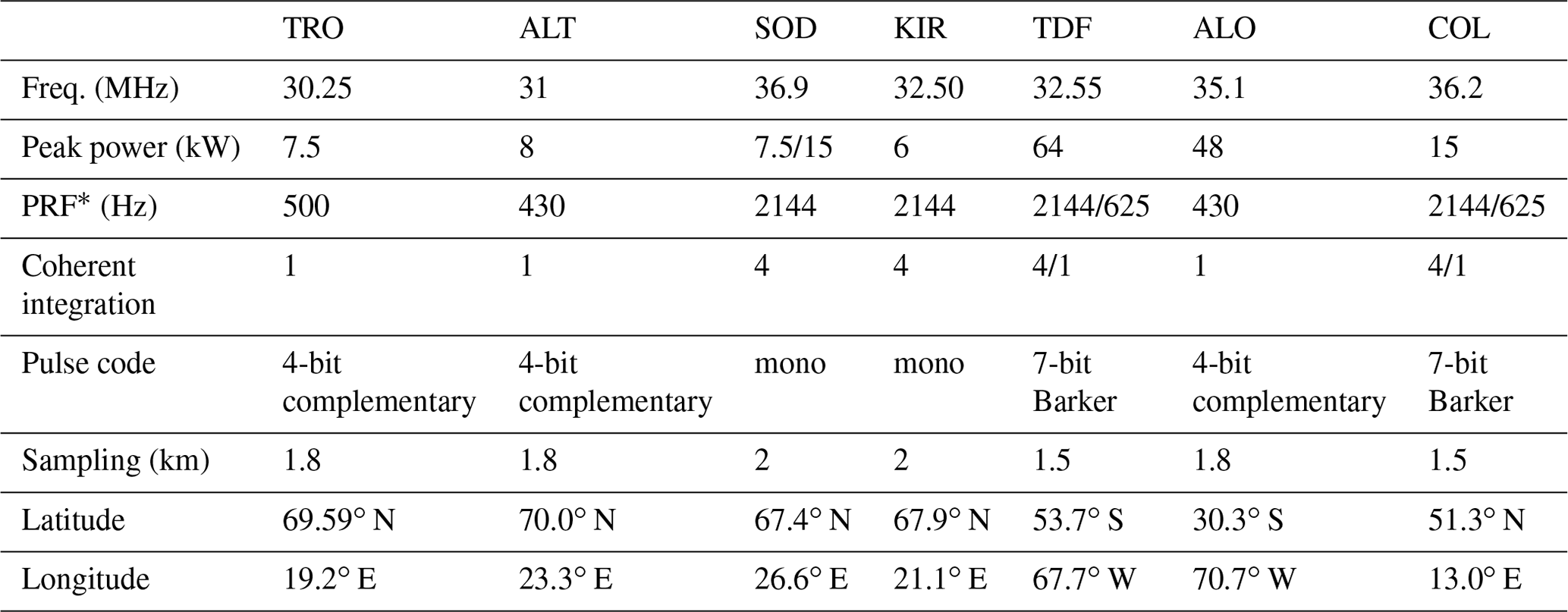
^∗ PRF: pulse repetition frequency.

MLT winds are obtained from meteor radar observations by applying a so-called all-sky fit (Hocking et al., 2001; Holdsworth et al., 2004), which minimizes the residuals of the projection of all radial or line-of-sight velocities onto a mean 3D wind within an altitude–time bin in a least-squares sense. The radial velocity equation is often written as

$$\begin{array}{}\text{(1)}& v_{\mathrm{r}}=u\cos \left(\mathit{\varphi }\right)\sin \left(\mathit{\theta }\right)+v\sin \left(\mathit{\varphi }\right)\sin \left(\mathit{\theta }\right)+w\cos \left(\mathit{\theta }\right).\end{array}$$

Here v_r is the line-of-sight velocity, u, v, and w represent the 3D wind velocities in the zonal, meridional, and vertical direction, θ denotes the zenith angle (also often referred to as the off-zenith angle), and ϕ is the azimuth angle counterclockwise from the east. In general, the vertical wind is assumed to be negligible (w = 0 m s⁻¹), which simplifies the equation to the horizontal wind components. Obviously, this assumption is justified considering the good agreement of the obtained horizontal winds when compared to meteorological analysis data (McCormack et al., 2017; Stober et al., 2020; Liu et al., 2020) and the large observation volume of about 350 km in diameter as well as the typical temporal resolution of 1 h.

Although it appears to be legitimate to make the simplification and to remove the vertical wind from the radial velocity equation, there is a need for a mathematical justification. Therefore, we investigate the bias that is intrinsic to meteor radar wind estimates by implementing different data analysis pipelines to the COL and TDF meteor radars using 3 months of data from January to March 2020. The first data analysis applies a least-squares fit using all three wind components, a nonlinear error propagation, and World Geodetic System 1984 (WGS84) geometry (National Imagery and Mapping Agency, 2000). The wind components are estimated by a singular value decomposition as a solver (Press et al., 1992). The second data analysis leverages the same observations, but all radial velocities were replaced by synthetic data, sustaining the spatial and temporal sampling of the original measurements and their corresponding statistical errors. The synthetic wind field is composed of an altitude-dependent mean wind, planetary waves, and tides plus some gravity waves. However, the vertical wind component was set to zero for all waves and the mean wind at all altitudes and times.

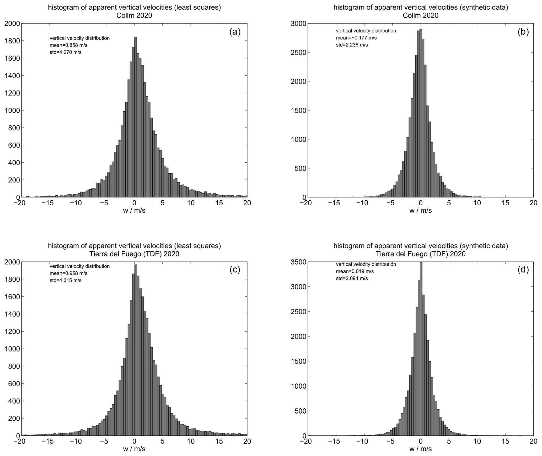
Figure 1 Histograms of the residual bias vertical velocities derived from the COL and TDF meteor radars using observations from January to March 2020. The left histograms (a, c) show the results of the hourly residual bias vertical velocities applying a least-squares fit. The right panels (b, d) show the resulting vertical velocities applying the same algorithm using the COL and TDF detections (volume sampling), but with synthetic data based on mean winds, planetary waves, and tides as well as a zero vertical velocity.

Figure 1 shows four histograms of hourly fitted vertical winds applying the classical least-squares approach to solve the radial wind equation. The left histograms present the vertical winds from our “naive” data analysis. The right panels visualize the vertical velocity distribution for the synthetic data; we put a zero vertical wind component for all waves. The histograms indicate rather large “apparent” vertical velocities. In particular, the analyzed synthetic data demonstrate that there are substantial biases (mostly related to the sampling, which results in large variances) considering the width of distribution, forming tails beyond a few meters per second (m s⁻¹). However, the synthetic data also exhibit a reduced standard deviation compared to the naive least-squares solutions, suggesting that there is at least some sensitivity left to “infer” a residual vertical wind from the observations. The difference between TDF and COL for the synthetic data is only related to the observational statistics. TDF has about twice the number of detections during this part of the season.

There are many reasons for the intrinsic bias in the meteor radar vertical winds. Some of them are almost impossible to address due to the lack of information provided by the current generation of meteor radars. For instance, the question arises of how fragmentation affects the radial velocity measurement and the interferometric solution. Trajectory information to correct for geometric offsets due to the specular and/or transverse scattering geometry is often not available. Recent studies of high-resolution optical observations indicated that almost 90 % of the observed meteors exhibit signs of fragmentation (Subasinghe et al., 2016; Vida et al., 2021). There is also the question of whether strong wind shear or turbulence induces an apparent motion of the scattering center along the trail axis. Most meteor radars lack the capabilities to investigate and quantify these effects in detail. Very few systems provide multistatic trajectory measurements, which are required to remove most of the wind shear and geometric effects (Webster et al., 2004; Jones et al., 2005; Brown et al., 2008b; Fritts et al., 2010b; Panka et al., 2021).

Another important aspect in the data analysis is related to the interferometric uncertainties of the angle of arrival (AoA). The receiver antenna array is typically arranged as an asymmetric cross with antenna spacing of 1λ and 1.5λ, 2λ and 2.5λ, or other combinations. Although such an array is often called a Jones array (Jones et al., 1998), it was developed and also applied in other disciplines (Rhodes et al., 1994). Interferometric solutions obtained from such arrays show errors of about 0.5–1^∘. These errors are included in the retrieval through a Gaussian error propagation in all quantities. Therefore, we adapted the procedure outlined in Gudadze et al. (2019). A more detailed discussion of the positions errors and the reliability of the forward scatter meteor radar observations can be found in Hocking (2018) and Zhong et al. (2021). Furthermore, small angular errors also result in altitude uncertainties. These measurement errors are mitigated by estimating the vertical shear from the spatiotemporal Laplace filter.

However, our synthetic data analysis points out that there are also mathematical and geometrical factors causing an intrinsic bias in the vertical velocities due to the spatial and temporal sampling. The synthetic data do not suffer from any disturbances related to the meteor trail physics. All radial velocities and their interferometric locations in the WGS84 coordinates are exactly determined, and only numerical and sampling aspects due to the time–altitude binning contribute to the standard deviation of the distribution shown in Fig. 1 (right panel). We also point out that the synthetic data use all statistical covariances and measurement errors as the real observations to ensure comparability on fair grounds. Furthermore, the radial wind equation is linear in all three wind components, which results in a weighted measurement response of the sin and cos terms for the zenith angles. Typical meteor radars detect most of the meteors at zenith angles between 55 and 65^∘, corresponding to a scale factor of 1.2 to 1.3 in the geometric measurement response between the horizontal components and the vertical wind. In addition, it is worth considering that the magnitude of the horizontal wind velocity is often more than a factor of 10 larger compared to the vertical wind magnitude. The consequence of these scaling terms is also reflected in the statistical uncertainties of the fitted wind coefficients, which range 2–12 m s⁻¹ or occasionally more than 15 m s⁻¹ for each coefficient. These statistical uncertainties are reasonable for horizontal winds, which very often exceed 20–40 m s⁻¹ as a mean wind speed, but are too large to retrieve physically and statistically sound solutions for the vertical velocities.

3 Bias related to scattering geometry

Transverse scatter or specular meteor radars are highly sensitive to the observation geometry. Full wave scattering simulations point out that there is a strong polarization dependence between the trail alignment and the polarization of the incident radio wave (Poulter and Baggaley, 1977; Stober et al., 2021c). The concept of meteor radar wind observation is based on the assumption that most of the backscattered radio energy originates from the specular point, which is assumed to be a well-defined location along an infinitely long ambipolar diffusing plasma column. However, the scattering point describes the motion of the scattering center rather than a well-defined location of the meteor trail. Thus, depending on the observing geometry, the measured Bragg vector denotes the motion of this scattering center, which is composed of the trail motion and apparent changes caused by the scattering geometry. These changes in the geometry are related to horizontal or vertical winds and wind shears, as well as electron line density variations caused by turbulence, fragmentation (Subasinghe et al., 2016; Vida et al., 2021), or differential ablation (Vondrak et al., 2008).

Figure 2 schematically illustrates how these apparent motions of the specular point relate to purely horizontal or vertical movements of the trail. The letter “A” describes the position of the specular point along the trail after the meteoroid passes the t₀ point (closest distance to the transmitter, see also McKinley, 1961; Hocking, 2000; Mazur et al., 2020), and “B” labels the location of this specular point if it stays “glued” to the trail, while the meteoric plasma column is drifted by the neutral wind. “C” labels the position of the scattering center considering the trail motion, but sustaining the geometry regarding the transmitter and receiver location (TX/RX). Although the concept of the specular point as a reflection center is already a substantial simplification of the scattering process, the scheme visualizes the basic geometric problem. A more realistic approach considers the fact that the scattering actually occurs from an extended section of the meteoric plasma trail along the meteor flight path containing several Fresnel zones around the specular point.

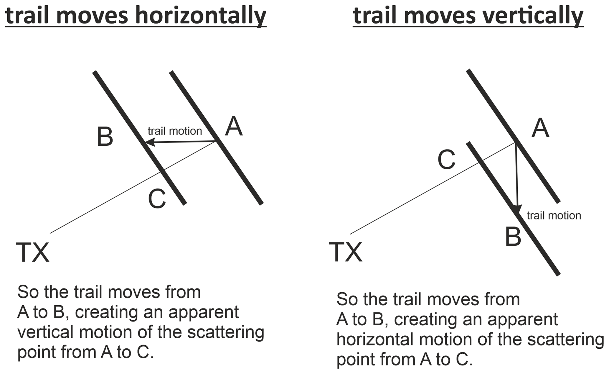
Figure 2 Idealized schemes of the specular scattering geometry indicating the apparent motion of the specular point or scattering center along the trail due to the drift of the meteor plasma column by neutral winds. The length of the meteoric trails is several kilometers, whereas the apparent motions of the scattering center are of the order of the meteor. The label ”A” shows the position of the specular point at the first detection, “B” denotes the location of the scattering center assuming it stays glued to the same mid-point of the trail, and “C” shows the position of the reflection point sustaining the transmitter and receiver geometry.

The latter point is of particular concern for multistatic or forward scatter meteor radar observations. Due to the larger angle between the incident radio wave and the meteoric plasma column, the scattering section along the trail is much longer. Stober and Chau (2015) already demonstrated that the forward scatter angle corresponds to a frequency shift to lower frequencies and thus to even larger Fresnel zones. Hence, changes in the electron line density within the scattering section along the trail act as an additional weighting and lead to even more pronounced apparent motions of the specular point, which can slide along the meteor trajectory. This sliding can be caused by changes in scattering geometry due to winds and wind shears or by modifications of the electron line density that are associated with fragmentation and differential ablation.

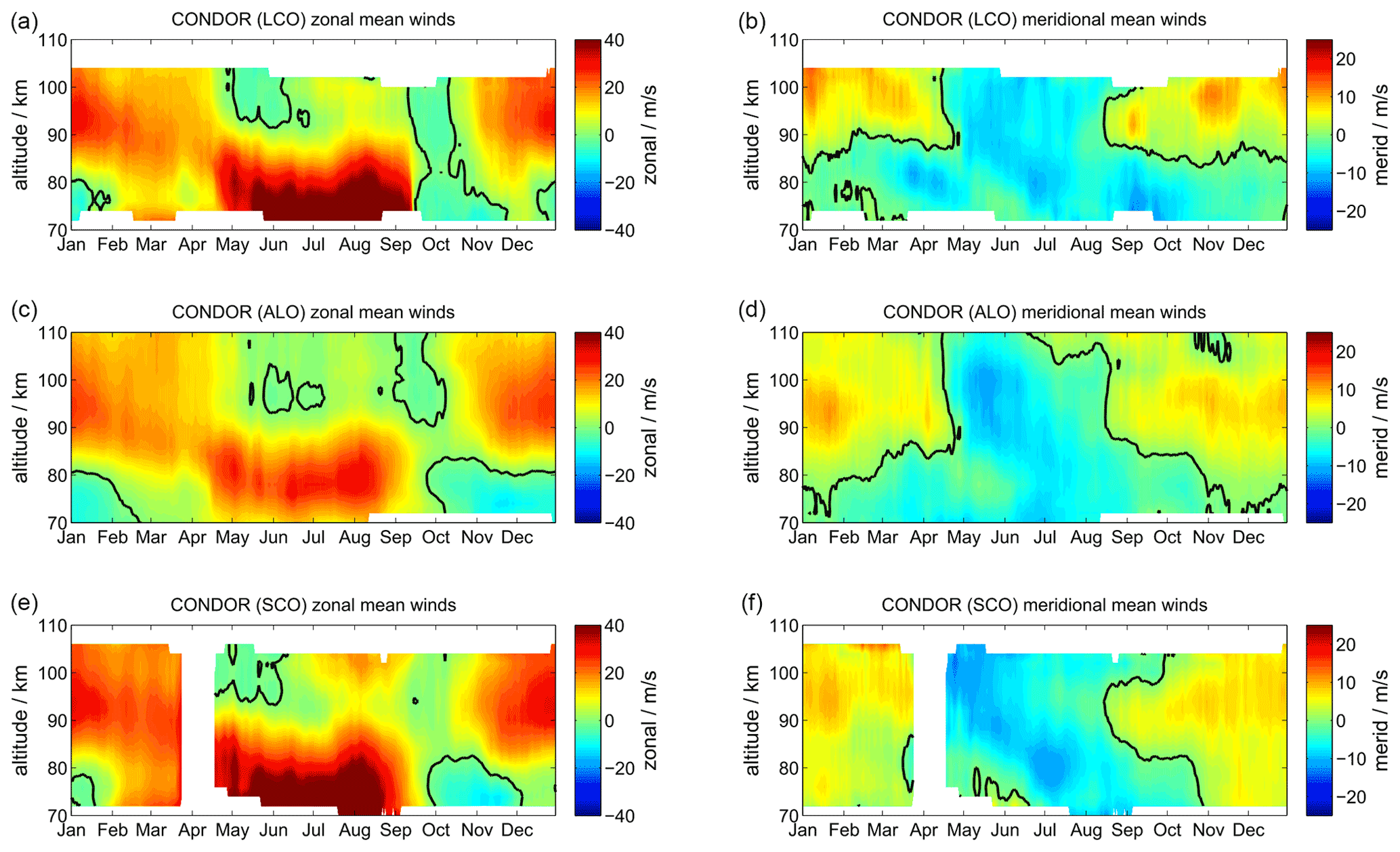
Figure 3 Comparison of zonal and meridional winds as a composite from 2012 to 2021 for the forward scatter receiver stations LCO and SCO as well as the monostatic radar in ALO. The left column (a, c, and e) shows the zonal wind component, and the panels on the right (b, d, and f) show the meridional wind. The panels are sorted according to their geographic latitude, with the northernmost sampling volume at LCO on top, the ALO in the center, and the southernmost station SCO in the lowest row.

We evaluate the hypothesis described above by performing a normal wind analysis using all three data sets provided by the CONDOR network in Chile. The network is unique in the sense that it combines a monostatic meteor radar and forward scatter passive receivers in a fairly compact geographic region. Figure 3 shows a comparison of the zonal (left column) and meridional (right column) winds using only the northernmost site at LCO, the standard meteor radar at ALO, and the passive receiver at SCO. A geographic map of all three sites can be found in Stober et al. (2021a). The observation volumes basically overlap to about 60 %, and thus it is reasonable to expect that a climatological comparison should result in almost identical mean wind behavior. However, zonal winds exhibit large differences, especially during May to September and at altitudes below 85 km. Above 85 km, discrepancies appear to be much smaller. The excess of the zonal wind magnitude between the monostatic (ALO) and the forward scatter stations is about a factor of 2 around 80 km and below. There is no geophysical reason why in such a narrow latitudinal band the zonal wind should show such significant changes. We reproduced these results with commercial software (Holdsworth et al., 2004) to rule out any issues caused by the retrieval algorithm that is described in detail in Sect. 4. It is evident from Fig. 3 that the zonal wind appears to be significantly stronger above the passive forward scatter receivers. Meridional winds seem to be much less affected, although there are substantial differences between the northernmost and southernmost location, which are only separated by 3^∘ in latitude. Our preliminary analysis thus already reveals that there is a considerable altitude-dependent difference in the wind magnitude between monostatic and passive receiver systems.

Finally, we investigate whether the magnitude difference also manifests in the Bragg vector pointing direction between the forward scatter receivers at SCO and LCO relative to the monostatic radar at ALO. In Fig. 2 we hypothesize that the Bragg vector pointing direction is not affected by the trail motion due to the wind, which is described by a parallel translation, and thus the Bragg vector pointing is supposed to remain perpendicular to the meteor trajectory for underdense meteors, whereas the length of the Bragg vector is a measure of the total path of the scattering center over successive radar pulses, which includes the motion of the trail due to the neutral wind plus an apparent sliding of the scattering center (specular point) along the trail.

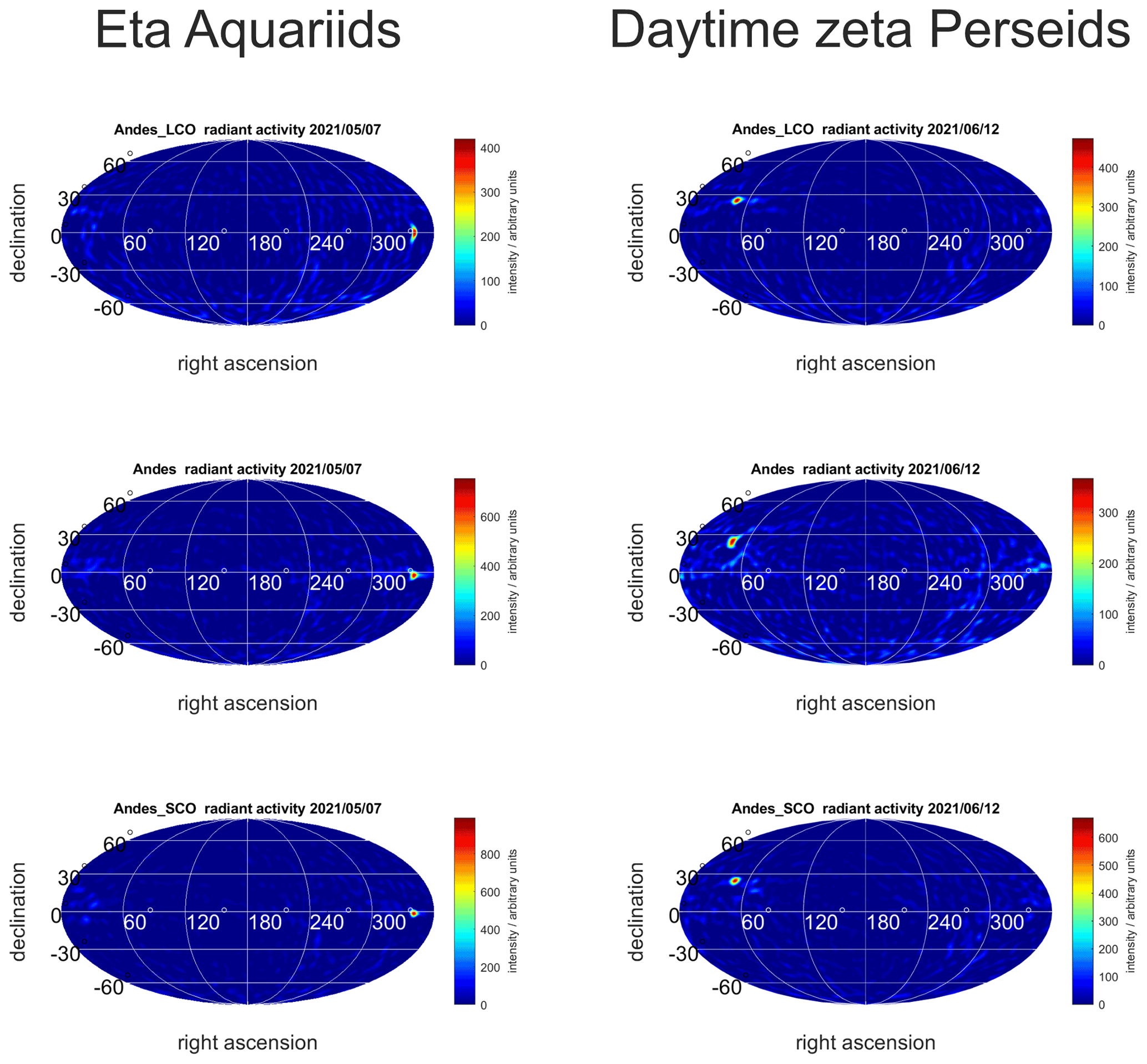
Figure 4 Meteor radiant activity maps derived from CONDOR for LCO, ALO (Andes), and SCO (the top, middle, and bottom row, respectively) . The left column shows the source radiant activity for the η Aquariids, and the right panels present the daytime zeta Perseids. The meteor showers are identified from the catalogues presented in Brown et al. (2010) and Janches et al. (2013).

We computed the source radiant of two well-known and long-lasting (several degrees in solar longitude) meteor showers by applying a modified single-station radiant mapping algorithm (Jones and Jones, 2006). The meteor source radiant maps for SCO, LCO, and ALO were obtained by implementing a revised version of the algorithm applied in Stober et al. (2013). The new generalized radiant mapping is based on the WGS84 geometry for each individual meteor. There have been already several meteor shower catalogues published in the literature covering the Northern and Southern Hemisphere (Brown et al., 2010; Janches et al., 2013; Pokorny et al., 2017), and hence it was easy to pick some of the established meteor showers for the solar longitudes of concern. Figure 4 shows six radiant activity maps for LCO, SCO, and ALO. At the beginning of May all three sites exhibit increased activity at the source radiant of the η Aquariids (ETA), which are visible at right ascension α = 337^∘ and declination δ = −0.9^∘. This meteor shower is active at solar longitudes of λ_sol = 30–60^∘, corresponding to the end of April until May (Brown et al., 2010; Janches et al., 2013). The second shower that we found was the daytime zeta Perseids (ZPE), which is visible at right ascension α = 56.6^∘ and declination δ = 23.2^∘. Daytime zeta Perseids are active at solar longitudes λ_sol = 56–90^∘, corresponding to the end of May until June (Brown et al., 2010; Schult et al., 2018). The right ascension and declination coordinates are provided for the days around the maximum meteor shower activity. These radiant activity maps indicate no systematic differences that explain the differences in the Bragg vector magnitudes between the forward scatter stations at SCO and LCO and the monostatic radar at ALO. More detailed position information for both meteor showers is presented in Appendix B1. Thus, the Bragg vectors are correctly determined for all stations and reflect no substantial deviation of the source radiant for these two meteor showers. In particular, the daytime zeta Perseids have a geocentric velocity of v_g = 28–32 km s⁻¹ and can hence penetrate deep into the atmosphere and reach the altitudes where we already see significant differences in the wind magnitudes. In summary, we were not able to identify a similar deviation in the source radiant mapping of two major meteor showers between the forward scatter receiver stations and the monostatic radar that corresponds to or explains the magnitude offset that is evident in the zonal winds.

4 Mathematical debiasing strategies

After we introduce the intrinsic bias of the vertical wind estimates in meteor radar observations, we are going to briefly discuss mathematical debiasing strategies. The most straightforward method is to implement a Tikhonov regularization in the least-squares fitting (Wilhelm et al., 2017; Stober et al., 2017). However, this approach leads to a brute-force norm reduction and depends on an empirically determined Tikhonov matrix and Lagrange multiplier:

$$\begin{array}{}\text{(2)}& {∥\mathbf{A}\mathit{x}-b∥}^{\mathrm{2}}+\mathit{\lambda }{∥\mathbf{\Gamma }\mathit{x}∥}^{\mathrm{2}}.\end{array}$$

Here A is the Jacobian matrix of the problem, x is our state vector, b represents the observations, Γ denotes the Tikhonov matrix, λ describes the Lagrange multiplier (here and further on λ=1), and the superscripts on the vertical lines denote the Euclidean norm. It is now possible to construct a Tikhonov matrix in such a way that $\underset{{\mathbf{\Gamma }}_{\mathrm{w}}\to \mathrm{\infty }}{lim}\mathbf{\Gamma }\mathit{x}\to \mathrm{\infty }$, which results in w = 0 m s⁻¹ for all solutions and is thus equivalent to the assumption of a negligible wind. The infinite growth of the right-hand side enforces a norm reduction for the vertical wind, and hence the vertical wind solution converges to zero. However, it is also possible to insert a solution of ${\mathbf{\Gamma }}_{\mathrm{w}}\in [\mathrm{0},\mathrm{\infty })$, which in consequence leads to a strong damping of the artificially large vertical velocities. The most straightforward approach is to use the identity matrix as the Tikhonov regularization, which is known as damped least squares but does not satisfactory remove the vertical wind bias.

Although a Tikhonov regularization is suitable to suppress artificially large vertical velocities, we are going to outline an even more complex approach to solve for the vertical wind. To this end, we modify the Tikhonov regularization to a filter function, which is also known as generalized Tikhonov regularization. Due to the implemented spatiotemporal Laplace filter in the meteor radar retrievals, it is straightforward to estimate a predictor for the state vector x_a for each time–altitude bin (Stober et al., 2020, 2021a). Furthermore, we can insert constraints to the error covariance for the state vector accounting for the scaling effects described above between the horizontal and vertical wind components. Thus, we now solve the problem using the form

$$\begin{array}{}\text{(3)}& {∥\mathbf{A}\mathit{x}-b∥}_{\mathbf{P}}^{\mathrm{2}}+\mathit{\lambda }{∥\widehat{\mathbf{\Gamma }}(\mathit{x}-{\mathit{x}}_{\mathrm{a}})∥}_Q^{\mathrm{2}}.\end{array}$$

Here, P denotes the inverse covariance matrix of b, and Q is the inverse covariance of x including a scaling term for the vertical wind component to remove the bias and again to remove the artificially large vertical velocities. The advantage of the new norm reduction is that for small differences x−x_a and reasonable covariance errors the solution is identical to the least-squares fit as the right-hand term of Eq. (3) basically vanishes. By construction the right-hand term permits a certain part of the solution to pass through the spatiotemporal Laplace filter depending on its covariance. The larger the statistical uncertainties, the stronger and more important the right-hand term becomes, which often results in smaller vertical velocities.

Furthermore, the spatiotemporal Laplace filter is also beneficial for the horizontal wind components to compensate for and reduce effects caused by the random and irregular spatial and temporal occurrence of meteors within the sampling (observation) volume of the radar. Sometimes, small or even tiny measurement errors in the location of a meteor may induce large projection errors in the final solution of the retrieved wind components, which is minimized and mitigated when applying the spatiotemporal filter.

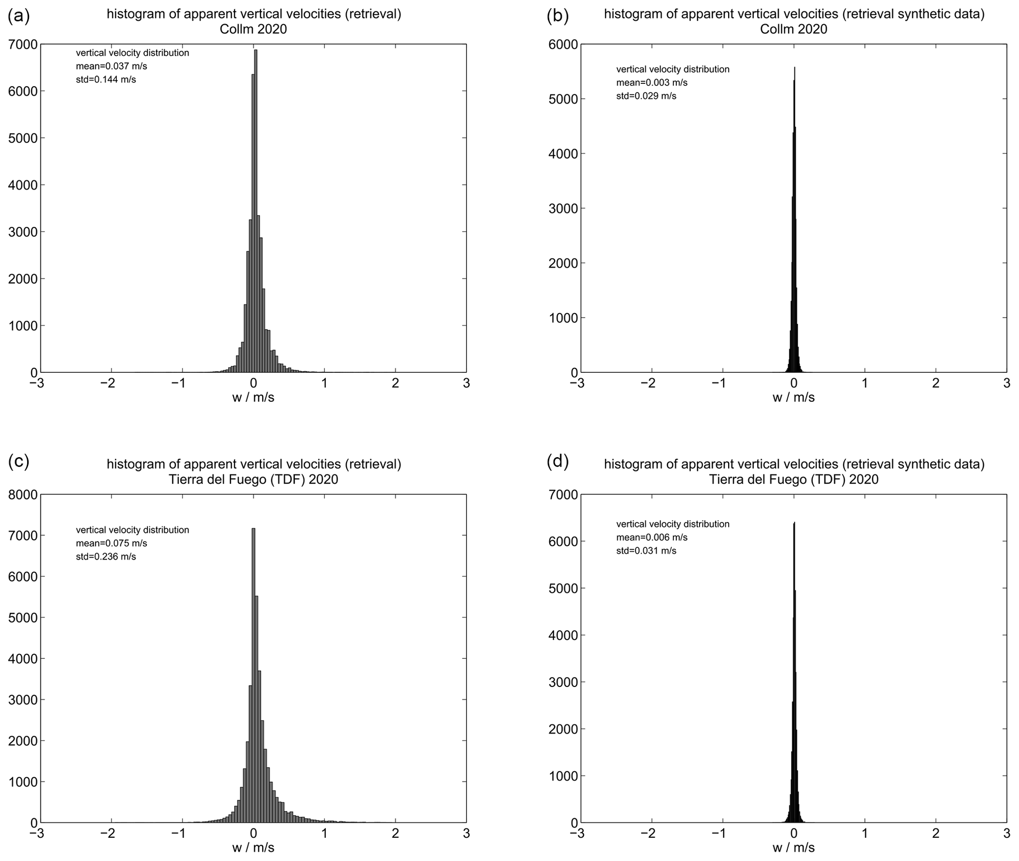
Figure 5 The same as Fig. 1, but the hourly vertical winds are obtained by applying the retrieval algorithm including the spatiotemporal Laplace algorithm. The x-axis scale or w-axis scale was reduced to show the remaining variability.

Figure 5 shows the vertical velocity histograms based on the retrieval algorithm applying the spatiotemporal Laplace filter and the empirical bias correction based on the scale analysis. The left panel shows the inferred vertical velocities based on the original COL and TDF observations. The histograms in the right panels are obtained when the synthetic data set, with all vertical wind values being zero, is analyzed with the retrieval algorithm. The remaining width of the distribution is caused by the sampling window in time and space (vertical bin size) as well as other atmospheric waves. However, this simple debiasing approach, whereby we just consider the scale analysis described above, substantially reduced the offset that was inherent when only a “standard” least-squares wind fit (Press et al., 1992) was applied (Fig. 1, right panel). Although generalized Tikhonov regularizations or filtering functions such as the spatiotemporal Laplace filter can help to reduce the intrinsic bias in the meteor radar wind analysis to determine vertical winds by comparing idealized synthetic data, we are still not able to prove the reliability of the derived vertical winds beyond their statistical properties due to a missing ground “truth”.

5 Statistical comparison to the non-hydrostatic UA-ICON model

A direct comparison of the retrieved vertical winds to other observations is not feasible due to the lack of such measurements. Therefore, we prepared a statistical comparison to a recently developed state-of-the-art non-hydrostatic general circulation model (GCM). The Upper Atmosphere ICOsahedral Non-hydrostatic (UA-ICON, Borchert et al., 2019) extends the vertical coverage of the ICON numerical weather prediction model from 80 km to about 150 km altitude. A detailed description of the upper atmosphere physics is given in Borchert et al. (2019). The upper atmosphere version leverages the numerical weather prediction physics packages (Zängl et al., 2015; Giorgetta et al., 2018; Crueger et al., 2018). Here we made use of a 21-year free-running climate simulation without any nudging and parameterized gravity waves on a so-called R2B4 grid with a horizontal resolution of 160 km (Borchert et al., 2019; Giorgetta et al., 2018). Above 120 km altitude the model applies Rayleigh damping to the vertical winds. The benefit of the UA-ICON model for such a comparison is that vertical winds are available on a geometric vertical coordinate grid. The UA-ICON horizontal winds and tides have been compared to WACCM-X(SD), GAIA, and data from six meteor radars (Stober et al., 2021b). Similar to this study we extracted vertical winds by considering the instrument observation volume.

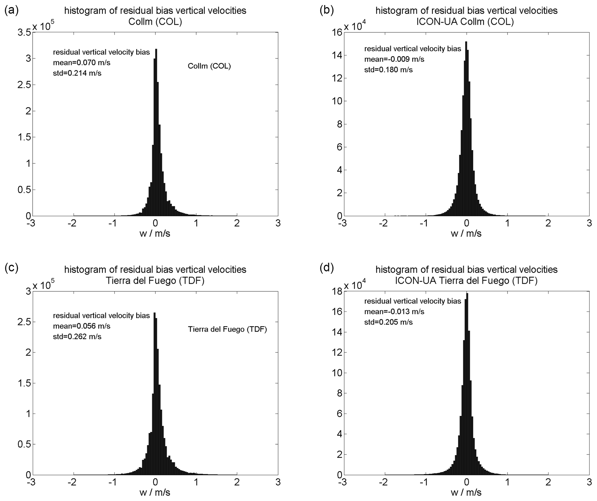
Figure 6 Histograms of the residual vertical velocity for the available data at COL and TDF including the debiasing from the spatiotemporal Laplace filter. The left panels (a, c) show the meteor radar observations. The right panels (b, d) visualize the corresponding UA-ICON velocities for a typical meteor radar sampling volume.

Figure 6 shows a statistical comparison of hourly retrieved vertical wind velocities for the COL and TDF meteor radars. These histograms are obtained using the entire available data set for both systems, which covers 16 years in the case of COL and about 12 years for TDF. The left column presents the observations from both meteor radars, and the right column shows the corresponding UA-ICON data. The histograms exhibit remarkable agreement of the inferred debiased vertical velocities. The observations, however, indicate more variability compared to the GCM. However, the overall agreement of the vertical velocity distribution between the observations and UA-ICON data reveals that at least the statistical moments of the distributions have significantly improved compared to the least-squares-derived vertical winds. Furthermore, it is possible to use the skewness of the histogram to estimate potential systematic issues of the radar due to either irregular detections within the radar beam volume or issues in the interferometric solution (e.g., technical problems). Although the debiasing seems to provide reasonable results, we cannot assess the reliability of individual observations or identify other systematic effects due to other more complicated scattering process (e.g., fragmentation, differential ablation, and so forth). Thus, we intend to go beyond these simple approaches and further refine the retrievals to implement physically and mathematically consistent solvers to infer more reliable vertical wind velocities and vertical wind variability.

6 3DVAR+DIV retrieval

Recently, a 3D-Var algorithm was introduced to retrieve spatially resolved 3D winds using multistatic meteor radar observations from the Nordic Meteor Radar Cluster and CONDOR (Stober et al., 2021a). This 3D-Var algorithm already included the retrieval of vertical winds but required a Tikhonov regularization to reduce the numerical instabilities, which often arise for parameters with low or poor measurement response. Due to the much worse statistics per grid cell, the quality of each radial velocity measurement comes even more into play and we have to consider the representativeness of a single measurement. This is achieved by introducing a smoothness constraint or variable correlation lengths inside the domain. Such correlation lengths are described by the averaging kernel. However, the zonal and meridional wind components exhibited a reasonable measurement response inside the retrieval domain with values beyond 0.6 and more, indicating short correlations or narrow averaging kernels. Another benefit of the 3D-Var approach was the possibility to add additional constraints by expanding the cost function, e.g., for data assimilation of other observations.

The new 3DVAR+DIV algorithm was revised and expanded by adding a divergence constraint to the cost function. For this, we implemented diagnostics to estimate the horizontal divergence and relative vorticity for each grid cell. We consider the fact that an air parcel that is moved by neutral winds should satisfy the continuity equation:

$$\begin{array}{}\text{(4)}& {\displaystyle \frac{\mathrm{d}\mathit{\rho }}{\mathrm{d}t}}+\mathit{\rho }\cdot \text{div}\left(\mathbf{u}\right)=\mathrm{0}.\end{array}$$

Here ρ is the mass density of the air, and we define a density operator in the following way:

$$\begin{array}{}\text{(5)}& {\displaystyle \frac{\mathrm{d}\mathit{\rho }}{\mathrm{d}t}}={\displaystyle \frac{\partial \mathit{\rho }}{\partial t}}+\mathbf{u}\cdot \text{div}\left(\mathit{\rho }\right).\end{array}$$

The spatial and temporal derivatives of the atmospheric density reflect the changes in temperature and pressure of an air parcel when a gravity wave or a whole gravity wave spectrum is present within the retrieval domain. Furthermore, the relative importance of each term in the continuity equation depends on the gravity wave properties. We performed a scale analysis for medium-frequency gravity waves ($N\gg \widehat{\mathit{\omega }}\gg f$) and estimated the deviation from the incompressible condition using the polarization relations given in Fritts et al. (2002) and Hocking et al. (2016). Here N denotes the Brunt–Väisälä frequency, $\widehat{\mathit{\omega }}$ is the intrinsic wave period, and f is the Coriolis parameter. The nonstationary and compressible terms are of the order of a few percent compared to ρ⋅div(u) term, which dominates by at least 1 or 2 orders of magnitude. More details are given in Appendix A. Having performed the scale analysis, it is reasonable to assume a stationary process for each time step, which is equivalent to $\mathrm{d}\mathit{\rho }/\mathrm{d}t=\mathrm{0}$. Thus, the continuity equation simplifies and we only have to derive the divergence for each voxel. The divergence is given in Cartesian coordinates by

$$\begin{array}{}\text{(6)}& \text{div}\left(\mathbf{u}\right)={\displaystyle \frac{\partial u}{\partial x}}+{\displaystyle \frac{\partial v}{\partial y}}+{\displaystyle \frac{\partial w}{\partial z}}=\mathrm{0}.\end{array}$$

In the 3D-Var algorithm, variable domain geometries could be used (Stober et al., 2021a). Therefore, the numerical solution of the derivatives to diagnose the horizontal divergence uses a first-order approximation of the elliptical integrals for the WGS84 reference coordinate systems (National Imagery and Mapping Agency, 2000), which appears to be sufficient for most of the typical voxel sizes of a few tens to hundreds of kilometers or a few degrees in latitude and longitude.

Assuming an incompressible flow, we can estimate the change in the vertical velocity Δw between two vertical layers and for each grid cell by

$$\begin{array}{}\text{(7)}& \mathrm{\Delta }{w}_i=\underset{z_{\mathrm{1}}}{\overset{z_{\mathrm{2}}}{\int }}\text{div}\cdot v_{h_i}\mathrm{d}z.\end{array}$$

Here the index i denotes the grid cell within a layer, and z₁ and z₂ are the upper and lower boundaries, respectively, describing the layer thickness.

The 3DVAR+DIV algorithm solves all equations through several iterations. The first call is again the standard 2D-Var retrieval; this permits us to obtain a first estimate of the horizontal divergence, which can be integrated for each grid cell assuming a lower boundary of the vertical velocity $w(z_{\mathrm{0}}{)}_{{\mathrm{0}}_i}$. From the second iteration, we include the continuity equation and perform the full 3DVAR+DIV retrieval.

To solve for the vertical velocity at each altitude and grid cell, we need to integrate Eq. (6) from below or above, which requires an initial value $w(z_{\mathrm{0}}{)}_{{\mathrm{0}}_i}$. Equation (6) only provides a relative measure for the change in the vertical velocity between two layers. The standard retrieval estimates this boundary in such a way that the mean vertical velocity (integrated over all altitudes) in each column for a defined domain grid is zero. This is equivalent to the assumption that the mean vertical motion in the column over large areas and a vertical dimension of approximately 20–40 km (thickness of the meteor layer) is close to zero.

However, the 3D-Var algorithm already included the full 3D wind solution for each grid and we just removed the Tikhonov regularization, which damped the numerical instabilities, in the new 3DVAR+DIV retrieval. These vertical velocities are called compressible–nonstationary solutions because we permit at least some deviation from zero in Eq. (5) without defining an explicit threshold. The major advantage of the 3DVAR+DIV retrieval is now given by providing a compressible–nonstationary and incompressible solution for the vertical velocity for each grid cell. The incompressible solution only makes use of the vertical velocity gradient obtained from the horizontal divergence equation to minimize the numerical instabilities caused by the low geometric measurement response in large parts of the domain. Thus, both solutions exhibit very similar morphology and only show some deviations in the absolute magnitude.

7 Results

The new 3DVAR+DIV retrieval is now implemented for routine data analysis for the Nordic Meteor Radar Cluster and CONDOR. The main goal was to infer more reliable vertical velocities using a more physically consistent data description in the forward model. The performance of the new algorithm is demonstrated using observations conducted during September 2021 after major upgrades of the TRO meteor radar. During this time of the year the circulation changes from typical summer conditions to the winter regime. There is moderate gravity wave activity, and enhanced semidiurnal tides are present (e.g.,  Wilhelm et al., 2019; Stober et al., 2021b).

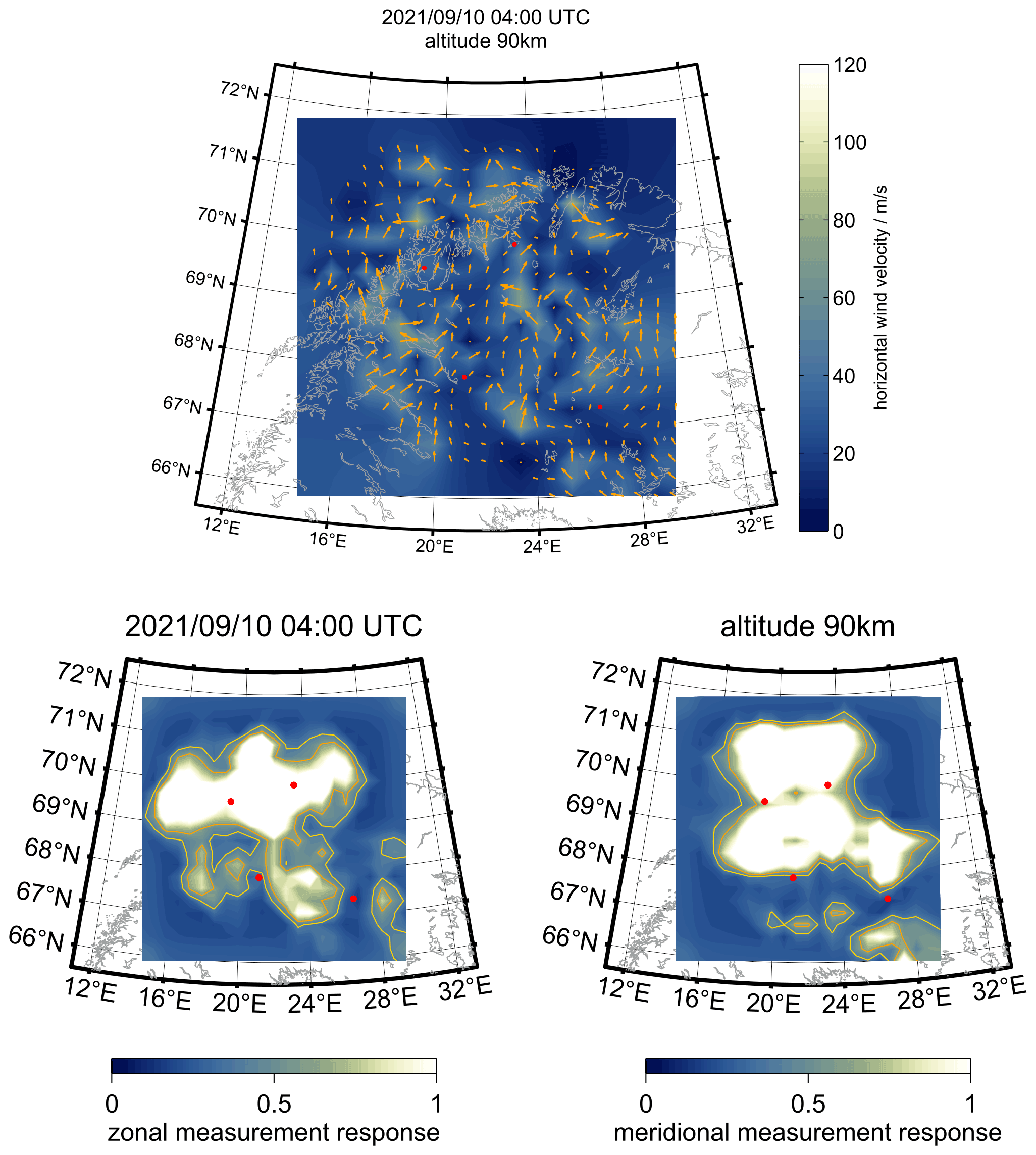
Figure 7 Snapshot of zonal and meridional winds as well as the corresponding measurement response using the 3DVAR+DIV algorithm and measurements from the Nordic Meteor Radar Cluster. The red dots label the locations of the meteor radars. The higher the measurement response, the better and brighter the colors. Bluish colors refer to long correlations, poor measurement statistics, and almost no information gain about small-scale dynamics.

The results presented herein are based on the 3DVAR+DIV algorithm using the Cartesian geographic grid with 30 km horizontal spacing, WGS84 geometry, a temporal resolution of 1 h, and a vertical spacing of 2 km. Figure 7 shows four panels. The upper panel shows the horizontal wind magnitude (color-coded) and the wind direction (orange arrows) for a single time bin and the altitude centered around 90 km. Black arrows represent the (horizontal) wind in grid cells that have enough meteor detections. The wind magnitude for each component is color-coded. Reddish colors refer to eastward and northward winds, whereas bluish colors indicate westward or southward motions, respectively. The lower two panels visualize the corresponding measurement response (Shannon, 1948; Shannon and Weaver, 1949; Stober et al., 2021a). The whiter the color, the higher the observation density, which allows high spatial resolution to be achieved. The bluer the grid cells are, the more information is mixed from long-distance correlations beyond the next neighboring grid cells corresponding to broader averaging kernels.

An essential improvement of the new 3DVAR+DIV algorithm is the embedded diagnostics of the horizontal divergence and relative vorticity between grid cells. These values are obtained by spatial derivatives qualitatively and quantitatively for all possible geometries and in both implemented domain grids (geographic and Cartesian, rectangular grid). We use Euler steps at the domain edges and central differences for all other grid cells within the domain. Figure 8 shows the horizontal divergence (left panel) and relative vorticity (right panel) for the same altitude and time period as the winds shown previously. The horizontal divergence exhibits coherent structures that are likely associated with a superposition of several gravity waves. A more random pattern is reflected by the relative vorticity, which shows a more patchy and irregular structure. Both quantities reach a relative strength of about ± 2 $\mathrm{m}{\mathrm{s}}^{-\mathrm{1}}{\mathrm{km}}^{-\mathrm{1}}$, and occasionally higher values were also found.

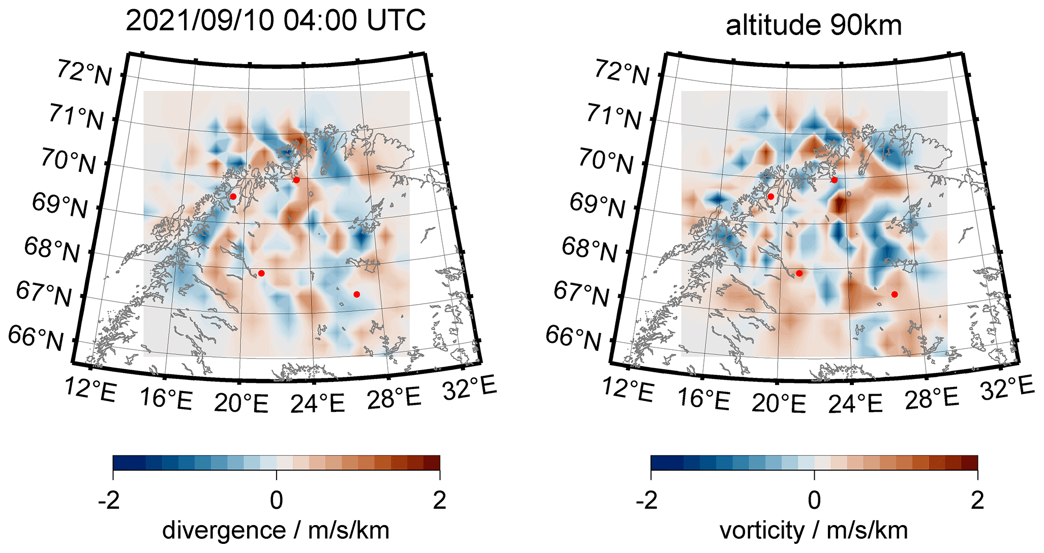
Figure 8 Horizontal divergence and relative vorticity calculated from the 3DVAR+DIV algorithm making use of the horizontal winds. The shown snapshot corresponds to the same period as in Fig. 7.

Finally, the retrieved vertical velocities (upper panels) and corresponding measurement responses (lower panels) are shown in Fig. 9. The absolute vertical velocities are obtained assuming a lower boundary, which was determined in such a way that the mean vertical velocity in the column above each grid cell is zero. The compressible–nonstationary and incompressible solutions for the vertical velocities are almost identical, which is very often the case. As our forward model makes use of the continuity and radial velocity equation, we have no independent estimate of the measurement response for the compressible–nonstationary solution, and only the residuals of the radial velocity equation contribute to the final estimate. Similar to the monostatic observations, the geometry of the meteor detections is not favorable to infer reliable vertical winds. Adding the continuity equation compensates for that but also dominates the measurement response and the overall contribution of the finally retrieved 3D winds. This is also reflected by the measurement response for the vertical velocities, which is identical for both solutions for the abovementioned reasons and is dominated by the horizontal velocity measurement responses.

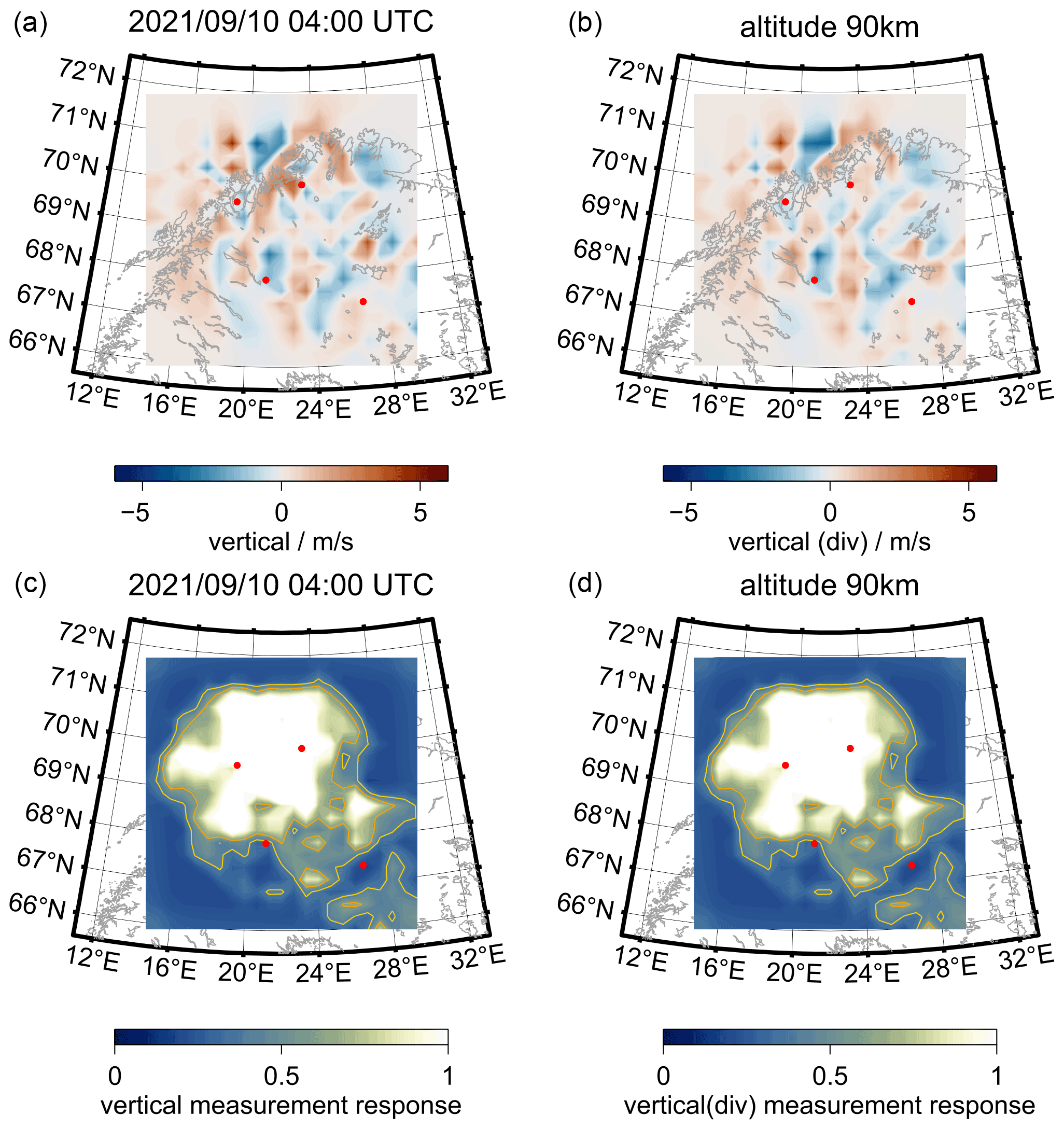
Figure 9 Corresponding vertical wind velocities (upper two panels, a and b) (a: compressible–nonstationary solution, b: incompressible solution) and measurement response (lower two panels, c and d) obtained by the 3DVAR+DIV algorithm for the same period as Fig. 7. Note that the measurement response of the compressible–nonstationary vertical wind solution is dominated by the incompressible solution, which is used in all iterations due to the implemented horizontal divergence constraint.

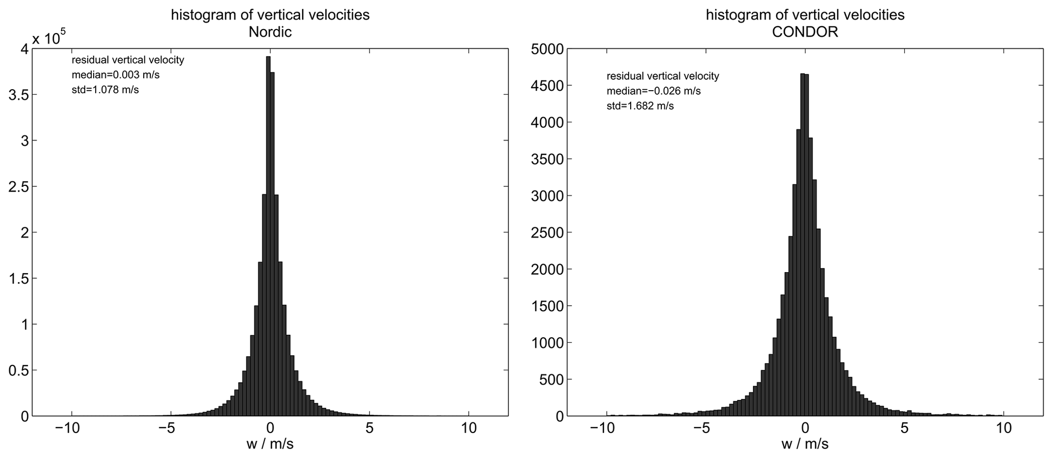
Figure 10 Histograms of hourly vertical winds obtained from the Nordic Meteor Radar Cluster and CONDOR.

We also investigated the statistical variability of the 3DVAR+DIV-derived vertical velocities. Therefore, we analyzed the year 2021 from the Nordic Meteor Radar Cluster and 2 weeks of data in March 2020 from CONDOR to estimate the statistical moments of the hourly inferred vertical wind measurements. The corresponding histograms are shown in Fig. 10. The histograms only contain results for grid cells with a measurement response larger than 0.5 for the compressible–nonstationary solution. The incompressible solution (vertical(div)) exhibits a few percent (< 11 %) reduced standard deviation for the same periods. The offset of the mean from zero is caused by the lower integration boundary condition being determined including all grid cells and altitudes, while the histograms only show a subset for all grid cells with a measurement response larger than 0.5. Furthermore, CONDOR shows a much higher variability compared to the Nordic Meteor Radar Cluster, which suggests that there is increased gravity wave activity above the Andes. Considering the different amount of data included in the histograms, we do not want to put too much focus on this difference in the vertical wind variability. Both histograms provide a sufficient database to infer the order of magnitude of the vertical wind variability for a 30 km diameter area. Increased variability is expected since this is significantly smaller than the typical monostatic observation volume.

8 Discussion

Vertical velocity measurements at the MLT are still very challenging. Since the first vertical wind observations performed with the Poker Flat mesosphere–stratosphere–troposphere (MST) radar in 1984 (Balsley and Riddle, 1984) using meteor echoes and scattering from coherent echoes, there have been many controversial discussions about potential biases. The results indicated a downwelling of about 30 cm s⁻¹ during the hemispheric summer at mesopause altitudes, whereas theoretical models predicted an upwelling of about 1 cm s⁻¹ to understand the cold mesopause temperatures (Holton, 1983). However, these observations also confirmed that the meridional winds were in agreement with the theory concerning the magnitude and sign. Later, Coy et al. (1986) proposed the Stokes drift to explain these observations, which basically decomposes the motion field in a Lagrangian and an Euler velocity component considering compressibility effects due to gravity waves. However, the Stokes drift crucially depends on the gravity wave properties, which alter the actual trajectory of an air parcel (Walterscheid and Hocking, 1991). Assuming a Garret–Munk type of gravity wave spectrum, the effect of a Stokes drift was estimated to be less than 4 cm s⁻¹ and thus not sufficient to explain the Poker Flat observations (Hall et al., 1992). Furthermore, it was hypothesized that the sedimentation speed of charged ice particles (plasma-laden aerosols) might be more suitable to explain the high negative vertical speeds. The vertical velocities presented here in applying the spatiotemporal Laplace filter and the 3DVAR+DIV algorithm reflect the Euler velocities and can be subject to Stokes drifts, which might explain seasonal differences of the mean velocities but is less critical for the vertical wind variability considering the results presented in Hall et al. (1992).

The most reliable observations have been carried out with high-power, large-aperture (HPLA) radars such as EISCAT and MAARSY (Hoppe and Fritts, 1995a, b; Fritts et al., 1990; Gudadze et al., 2019). However, these observations still indicated biases when attempting to infer absolute magnitudes close to zero. Some of these biases appear to be caused by gravity waves, as was reported for the EISCAT measurements. MAARSY results indicated a remaining uncertainty due to scattering from PMSE related to the sedimentation speed of the ice particles (Gudadze et al., 2019), which is in agreement with the arguments presented in Hall et al. (1992). However, HPLA radar measurements provide at least some valuable insights on the vertical wind variability and the magnitude of the vertical winds for the characteristic beam volumes and dwell times of the systems (seconds to minutes). These radars achieve statistical uncertainties down to a few centimeters per second (cm s⁻¹) of the line-of-sight velocities, which is sufficient for most geophysical processes (Stober et al., 2018) but still leaves some ambiguities when it comes to the very small vertical velocities related to the residual circulation (e.g., Holton, 1983; Smith, 2012; Becker, 2012, and references therein) .

There have been some attempts to derive mean vertical velocities from meteor radar observations by applying least-squares fits (Egito et al., 2016; Conte et al., 2021). These meteor radar observations clearly exhibit intrinsic biases that can result in artificially large vertical velocities of more than a few meters per second (m s⁻¹). In particular, Conte et al. (2021) reported vertical velocities in excess of ± 10 m s⁻¹ over hours. Considering the large observation volume of a few hundred kilometers for a typical domain area for multistatic observations, these values seem to be very large. Furthermore, based on measurements presented in this study using data from the Nordic Meteor Radar Cluster and CONDOR, we were not able to reproduce these extreme values using the 3DVAR+DIV algorithm analyzing more than 2 years of data. Although there could be various reasons for such large values, we were able to identify some intrinsic biases related to the observation geometry and sampling and present mathematical debiasing strategies for monostatic meteor radars using synthetic data. The proposed Tikhonov regularization and generalized Tikhonov or filter functions provide statistically sound solutions for the vertical winds by mitigating geometrical or numerical issues related to the least-squares analysis. Furthermore, we also want to point out that since the assumption of a zero vertical wind seems to be justified in the context of these biases, this approach is mathematically equivalent to a Tikhonov regularization. In addition, artificially large vertical velocities can degrade the quality of the horizontal wind solutions and also affect other analyses such as momentum fluxes.

The comparison of the statistical distribution of vertical velocities inferred from meteor radar observations and the UA-ICON model gives some confidence that the applied debiasing results in more consistent solutions for this wind component. However, there are still some sources of error left (e.g., fragmentation, motion of scattering center along the trail), which let us conclude that the term “residual bias vertical velocity” or “apparent vertical velocity” seems to be the right term as we cannot prove the correctness of individual hourly measurements. Fragmentation of the meteoroids as well as mean winds and wind shears can lead to small changes in the scattering geometry, which cause an apparent shift of the scattering center along the trail. Thus, the Bragg vector of the scattered electromagnetic wave is not necessarily defined by the motion of the trail due to neutral winds. Although these changes appear to be small, they affect the vertical component much more than the horizontal winds. In particular, these apparent motions of the scattering center along the trail could occur for transition echoes from overdense to underdense, which could be caused by fragmentation (Subasinghe et al., 2016; Vida et al., 2021) or by differential ablation (Vondrak et al., 2008).

Almost a decade ago, there was a lidar study on vertical wind magnitudes related to atmospheric tides (Yuan et al., 2014). The climatology exhibited vertical velocities of a few centimeters per second (cm s⁻¹) for large-scale atmospheric tidal waves. The lidar observations indicated about 15–20 cm s⁻¹ vertical wind magnitude for the semidiurnal tide and about 5–10 cm s⁻¹ for the diurnal tide. These values appear to be consistent with the apparent vertical velocities estimated for the monostatic meteor radars at COL and TDF applying the spatiotemporal Laplace filter. The midlatitude stations are dominated by semidiurnal tides during the hemispheric winter season and diurnal tides during the summer months (Stober et al., 2021b). However, the vertical wind magnitudes presented by Yuan et al. (2014) and in this study are orders of magnitude lower than other estimates obtained from meteor radar observations (Egito et al., 2016) and multistatic meteor radar data (Chau et al., 2017, 2021; Conte et al., 2021).

Furthermore, we investigated systematic differences in the derived neutral wind velocities using data from CONDOR only. The comparison reveals a considerable difference in the estimated total wind magnitude during several months from May to August at altitudes below 85 km. The difference is most prominently visible in the zonal wind, but the meridional wind is also affected, which is less obvious due to the much lower mean wind speeds. However, our radiant activity mapping of two meteor showers supports the scheme described above of a sliding scattering center or specular point along the meteor trajectory due to the motion of the trail by neutral winds. The source radiant maps only depend on the accurate determination of the pointing direction of the Bragg vector and are thus not affected by the apparent scaling of its magnitude due to the sliding of the scattering center along the meteor trajectory. Forward scatter receivers are more prone to this effect. Tiny changes in the geometry result in comparably larger apparent motions of the scattering center compared to monostatic systems. Furthermore, the effect increases the longer the trail lasts, corresponding to a slower diffusion, and thus the lower altitudes are mostly affected. However, the discovered bias in CONDOR between the monostatic and forward scatter mean winds is worth investigating in more detail and opens the question of how to interpret the Bragg vector and corresponding radial motion concerning the specular or transverse scattering and the meteor trail geometry.

Multistatic observations are versatile and new approaches can be applied to improve vertical wind measurements. Considering the fast development over the past years from the first multistatic forward scatter meteor radar experiment (Stober and Chau, 2015) to more routine and established networks (Chau et al., 2017; Spargo et al., 2019) underlines the huge scientific potential of such observations. These first observations were analyzed by making use of the classical assumptions on the vertical velocity (w = 0 m s⁻¹) or by fitting a mean value within the observation volume (Stober and Chau, 2015; Chau et al., 2017). However, the retrieval of vertical winds remained challenging even when more advanced methods were applied (Volz et al., 2021). These advanced methods still resulted in vertical wind velocities of up to 10 m s⁻¹ or more. The 3D-Var retrieval controlled the numerical instability in the vertical velocities by a Tikhonov regularization for each grid cell (Stober et al., 2021a). The new 3DVAR+DIV approach circumvents the need for an additional Tikhonov regularization by extending the forward model with the continuity equation, which permits the estimation of horizontal divergence and relative vorticity directly to constrain the vertical velocity solution.

The algorithm permits us to obtain a compressible–nonstationary and incompressible solution for the vertical winds. Furthermore, the combined radial velocity and continuity equations leverage the good measurement response from the horizontal wind velocities, which significantly increases the measurement response for the vertical velocities as well. Due to the much smaller scales that are resolvable with the 3DVAR+DIV retrieval compared to standard monostatic meteor radars, it can be expected that a higher variability and larger vertical wind magnitudes might be observable. The values obtained from the new retrieval fit between the large-scale values from the monostatic retrievals and observations using HPLA radars (Hoppe and Fritts, 1995a; Fritts et al., 1990; Gudadze et al., 2019), which represents the limit for the smallest temporal scales of a few seconds (dwell time) and a spatial coverage of 3–4 km (beam diameter). Furthermore, we tested the 3DVAR+DIV retrieval with a much higher temporal resolution of 10 min. At this resolution the compressible solution again showed signs of numerical instability due to the much sparser data coverage, which can be compensated for by increasing the Lagrange multiplier for the vertical covariance constraint at the cost of smoothing some small-scale structures. A similar effect occurs when increasing the vertical bin size beyond the typical 2 km. Due to the large vertical shear often associated with large-scale waves such as tides, this increases the tendency for numerical instability, which in turn has a negative effect on the reliability of vertical winds.

One aspect is left that is worth consideration. The vertical integration of the horizontal divergence, which is needed to derive absolute vertical velocities, requires an initial boundary condition either at the bottom or top side of the domain depending on the integration direction. Currently this boundary is estimated assuming that the mean vertical velocity in each column above a grid cell is zero. We also tested domain means and other options. These values for the vertical velocity at the lower boundary are typically smaller than ± 0.2–0.3 m s⁻¹ for hourly winds. These vertical velocities are fairly consistent compared to other studies estimating vertical winds at altitudes of 70–80 km (Straub et al., 2012; Vincent et al., 2019), which are representative for a coarser temporal resolution of several hours to a day. Thus, the new 3DVAR+DIV retrieval provides more reliable values of the vertical wind variability rather than absolute wind values at a specific altitude.

Furthermore, the combined horizontal divergence and vertical velocities present good additional diagnostics to identify coherent structures in the domain area, which can be associated with gravity waves. This is often more difficult to achieve from the horizontal winds alone without additional filtering. Zonal and meridional winds are dominated by large-scale waves such as atmospheric tides that gain large magnitudes and thus lead to apparently smooth color maps and mostly parallel wind arrows in the images.

9 Conclusions

In this study we outlined some of the intrinsic biases that arise when inferring vertical winds from standard monostatic and multistatic meteor radar observations. For this purpose, we implemented a data analysis pipeline based on least-squares fits with a singular value decomposition solver for real and synthetic data. We demonstrated that even for synthetic data with zero vertical winds in all atmospheric components including mean winds, planetary waves, tides, and gravity waves, a least-squares analysis results in artificially large vertical winds with a standard deviation of ± 2.3 m s⁻¹. For real atmospheric soundings the standard deviation had a value of up to ± 5 m s⁻¹. This bias is caused by the temporal and spatial sampling of meteor radars due to the random occurrence of meteors inside the beam volume of about 350 km in diameter. Every meteor observation is representative of a given time period determined by the decay time of ambipolarly diffusing meteoric plasma and the spatial extension of the scattering volume along the trail. Thus, the apparent line-of-sight velocities are representative of a well-defined area inside the beam volume defined by the Fresnel scattering and for a very short time period, which is typically less than a second.

Considering these sampling aspects for typical meteor radar observations, we introduced two mathematical debiasing strategies to ensure that the estimated wind components are statistically sound solutions for a given spatial and temporal meteor distribution within each time–altitude bin. We showed that the assumption of a zero vertical wind, which is often used in standard meteor radar wind analysis algorithms, is equivalent to a Tikhonov regularization of the solution for an infinitely large vertical wind component in the Tikhonov matrix. Furthermore, we introduced a more complex approach by designing a spatiotemporal Laplace filter with constraints on the error covariance, which can be seen in the broadest sense as a generalized Tikhonov regularization. This retrieval algorithm resulted in a standard deviation for the same synthetic data set of ± 3 mm s⁻¹. In addition, we analyzed available multiyear meteor observations from COL and TDF and performed a statistical comparison of the inferred vertical winds with those from the UA-ICON model. The mean and statistical moments of the resultant vertical velocity distributions showed surprisingly good agreement concerning the GCM. However, we are not able to prove the geophysical correctness of the computed vertical wind for individual measurements, which is why we conclude that the term “residual bias vertical winds” or “apparent vertical velocity” still seems to be justified.

Although specular or transverse scatter meteor radars have been in use for decades, there is still some debate about the scattering mechanism and whether there are additional geometry effects due to the high aspect sensitivity of meteor trails. Recent quantitative simulations of reflection coefficients with a full wave scattering model have confirmed a significant change in the effective decay time and signal magnitude, which depends on the polarization of the incident radio wave and the meteor trail alignment (Stober et al., 2021c). We were able to identify another bias in the wind magnitude when comparing forward scatter receiver data and monostatic observations using CONDOR. The bias appears to be most significant below 85 km and increases with decreasing altitude. We explain this offset by a sliding of the scattering center along the meteor trail when the meteoric plasma column drifts with the neutral winds. Thus, meteor radars measure the Doppler velocity of the scattering center or specular point, which consists of the “true” Doppler from the neutral winds and an apparent velocity component caused by an apparent motion of the scattering center along the trail. Source radiant mapping of two meteor showers confirmed that the Bragg vector pointing direction remained unaffected. Most existing meteor radars do not provide information on the meteor orbit or trajectory, and thus this bias poses an additional challenge to estimate mean vertical winds from monostatic or isolated forward scatter meteor radars. However, for meteor radar networks with overlapping beam volumes the 3DVAR+DIV algorithm compensates for some of the remaining issues.

The new 3DVAR+DIV algorithm for multistatic meteor radar networks was implemented for routine data analysis of CONDOR and Nordic Meteor Radar Cluster observations. This algorithm provides the first physically and mathematically consistent approach to infer vertical velocities and vertical velocity variability from multistatic networks by combining the continuity and radial velocity equations in the cost function. Furthermore, the 3DVAR+DIV retrieval includes new diagnostics such as horizontal divergence and relative vorticity for each grid cell. In particular, the horizontal divergence benefits from the good measurement response of the horizontal wind components, and thus the vertical velocities derived from the incompressible solution also reflect a high measurement response. The derived vertical velocities are in the range of w = 1–2 m s⁻¹ and sometimes (3–4 standard deviations) exceed 3–4 m s⁻¹ for single grid cells of 30×30 km and a temporal resolution of 1 h. Due to the vertical integration of the continuity equation, the absolute magnitude is still subject to the assumption that the mean vertical velocity over a large vertical and spatial column is small. Although the mean absolute value still depends on the upper and lower boundary, the horizontal divergence and vertical wind variability are robust quantities and provide valuable information about the spatial scales of gravity waves and their horizontal wavelength spectra. Furthermore, we are able to estimate the degree of deviation from the incompressibility for medium-frequency gravity waves by leveraging linear theory and polarization relations of gravity waves. These deviations were of the order of a few percent, and thus the 3DVAR+DIV algorithm vertical winds should be reliable and robust to at least provide solutions of the right order of magnitude for retrieved spatial and temporal scales.

Appendix A: Scale analysis of compressibility effects in the continuity equation for medium-frequency gravity waves

In the following, we are going to briefly outline a scale analysis about the leading terms in the continuity equation to justify the incompressibility constraint and also to estimate the potential deviations for the compressible–nonstationary solution of the vertical winds. This scale analysis is valid for medium-frequency gravity waves. A more detailed theoretical description of the fundamental fluid dynamic equations can be found in Holton (1982). Reviews about the linear theory on gravity waves in the middle atmosphere can be found in Fritts et al. (2002) and Hocking et al. (2016).

$$\begin{array}{}\text{(A1)}& {\displaystyle \frac{\mathrm{d}\mathit{\rho }}{\mathrm{d}t}}+\mathit{\rho }\cdot \text{div}\left(\mathbf{u}\right)=\mathrm{0}\text{(A2)}& {\displaystyle \frac{\partial \mathit{\rho }}{\partial t}}+\mathbf{u}\cdot \text{div}\left(\mathit{\rho }\right)+\mathit{\rho }\cdot \text{div}\left(\mathbf{u}\right)=\mathrm{0}\end{array}$$

Consider that a monochromatic gravity wave can be written as

$$\begin{array}{}\text{(A3)}& \begin{array}{rl}& \mathit{\rho }={\mathit{\rho }}^{\prime }{e}^{i(kx+mz-\mathit{\omega }t)},\\ & u=u^{\prime }{e}^{i(kx+mz-\mathit{\omega }t)},\\ & v=v^{\prime }{e}^{i(kx+mz-\mathit{\omega }t)},\\ & w=w^{\prime }{e}^{i(kx+mz-\mathit{\omega }t)},\\ & \mathit{\theta }={\mathit{\theta }}^{\prime }{e}^{i(kx+mz-\mathit{\omega }t)}.\end{array}\end{array}$$

Here k is the horizontal wave number, Θ is the potential temperature, m is the vertical wave number, which can be complex, and ω describes the intrinsic wave angular frequency. The quantities ${\mathit{\rho }}^{\prime },u^{\prime },v^{\prime },w^{\prime }$, and θ^′ denote the wave amplitude. Furthermore, we introduce a background atmospheric density ρ₀, potential temperature Θ₀, and a wind field u₀. When we now insert the ansatz of a monochromatic wave in the continuity equation, we obtain

$$\begin{array}{}\text{(A4)}& -i\mathit{\omega }{\mathit{\rho }}^{\prime }+{\mathbf{u}}_{\mathrm{0}}(ik{\mathit{\rho }}^{\prime }+im{\mathit{\rho }}^{\prime })+{\mathit{\rho }}_{\mathrm{0}}(ik{u}^{\prime }+im{w}^{\prime })=\mathrm{0}.\end{array}$$

Furthermore, we make use of the fundamental fluid dynamic equations for a uniform hydrostatic background state:

$$\begin{array}{}\text{(A5)}& {\displaystyle \frac{\mathrm{d}}{\mathrm{d}t}}{\displaystyle \frac{\mathit{\theta }}{{\mathit{\theta }}_{\mathrm{0}}}}+w^{\prime }{\displaystyle \frac{N^{\mathrm{2}}}{g}}=\mathrm{0}.\end{array}$$

Considering the relation between potential temperature, pressure, and density,

$$\begin{array}{}\text{(A6)}& {\displaystyle \frac{\mathit{\theta }}{{\mathit{\theta }}_{\mathrm{0}}}}={\displaystyle \frac{\mathrm{1}}{c_s^{\mathrm{2}}}}{\displaystyle \frac{p}{p_{\mathrm{0}}}}-{\displaystyle \frac{\mathit{\rho }}{{\mathit{\rho }}_{\mathrm{0}}}},\end{array}$$

and taking $\underset{c_s\to \mathrm{\infty }}{lim}\frac{\mathrm{1}}{c_s^{\mathrm{2}}}=\mathrm{0}$ results in

$$\begin{array}{}\text{(A7)}& {\displaystyle \frac{\mathrm{1}}{{\mathit{\rho }}_{\mathrm{0}}}}{\displaystyle \frac{\mathrm{d}}{\mathrm{d}t}}\mathit{\rho }+w^{\prime }{\displaystyle \frac{N^{\mathrm{2}}}{g}}=\mathrm{0}.\end{array}$$

Using solutions of a monochromatic gravity wave in Eq. (A7), we find

$$\begin{array}{}\text{(A8)}& i\mathit{\omega }{\displaystyle \frac{{\mathit{\rho }}^{\prime }}{{\mathit{\rho }}_{\mathrm{0}}}}+w^{\prime }{\displaystyle \frac{N^{\mathrm{2}}}{g}}=\mathrm{0}.\end{array}$$

Now we focus on a comparison of the amplitudes between the density variation and the vertical winds, and we make use of the polarization relation for a medium-frequency gravity wave according to linear theory (Fritts et al., 2002; Hocking et al., 2016), which leads to the following relation:

$$\begin{array}{}\text{(A9)}& {\mathit{\rho }}^{\prime }={\displaystyle \frac{k{u}^{\prime }{N}^{\mathrm{2}}}{m\mathit{\omega }g}}{\mathit{\rho }}_{\mathrm{0}}.\end{array}$$

Finally, we can insert Eq. (A9) in Eq. (A4) and express all terms as a function of the intrinsic wave properties assuming a background wind field in the form ${\mathbf{u}}_{\mathrm{0}}=(u_{\mathrm{0}},\mathrm{0},\mathrm{0})$. Furthermore, we assume that the mean zonal background wind is comparable to the gravity wave fluctuation ($u_{\mathrm{0}}\approx u^{\prime }$), which simplifies the final scale analysis but has no impact on the results. Neglecting the mean vertical wind also has no impact as at most this term could gain the same magnitude as the horizontal wind component. Considering these background boundary conditions in Eq. (A4), we obtain

$$\begin{array}{}\text{(A10)}& \underset{A}{\underbrace{{\displaystyle \frac{\mathit{\omega }{u}^{\prime }N}{g}}}}+\underset{B}{\underbrace{{\displaystyle \frac{k{u}^{\prime \mathrm{2}}N}{g}}}}+\underset{C}{\underbrace{\mathrm{2}{u}^{\prime }k}}=\mathrm{0}.\end{array}$$

Finally, we estimate the relative importance of the terms A, B, and C. The term $A/C$ is comparably small for all medium-frequency gravity waves; it remains below 1 % and only gains a relative importance of up to 10 % for wave periods approaching the Brunt–Väsiälä frequency. However, such gravity waves no longer fall into the medium-frequency range and thus need to be considered for much higher-temporal-resolution retrievals than those presented herein. The ratio $B/C$ basically does not exceed 3 % over a wide range of horizontal wavelengths 30–1000 km and the background atmospheric conditions at the mesosphere and lower thermosphere.

Appendix B: Source radiant

The location of both meteor showers on the celestial sphere was determined using the tracking algorithm presented in Stober et al. (2013). The error bars denote the width of the stream corresponding to the full width at half-maximum. The mean difference between the right ascension and declination is less than 2^∘, and there is no additional dispersion visible when comparing the monostatic meteor radar observations and the passive receivers. Figure B1 was obtained using all solar longitudes with meteor shower activity exceeding 100 in arbitrary units. Hence, there are also solar longitudes included for which the shower was only visible in one of the systems. The radiant motion in celestial coordinates shows the typical shower drift with time and solar longitude (data not shown).

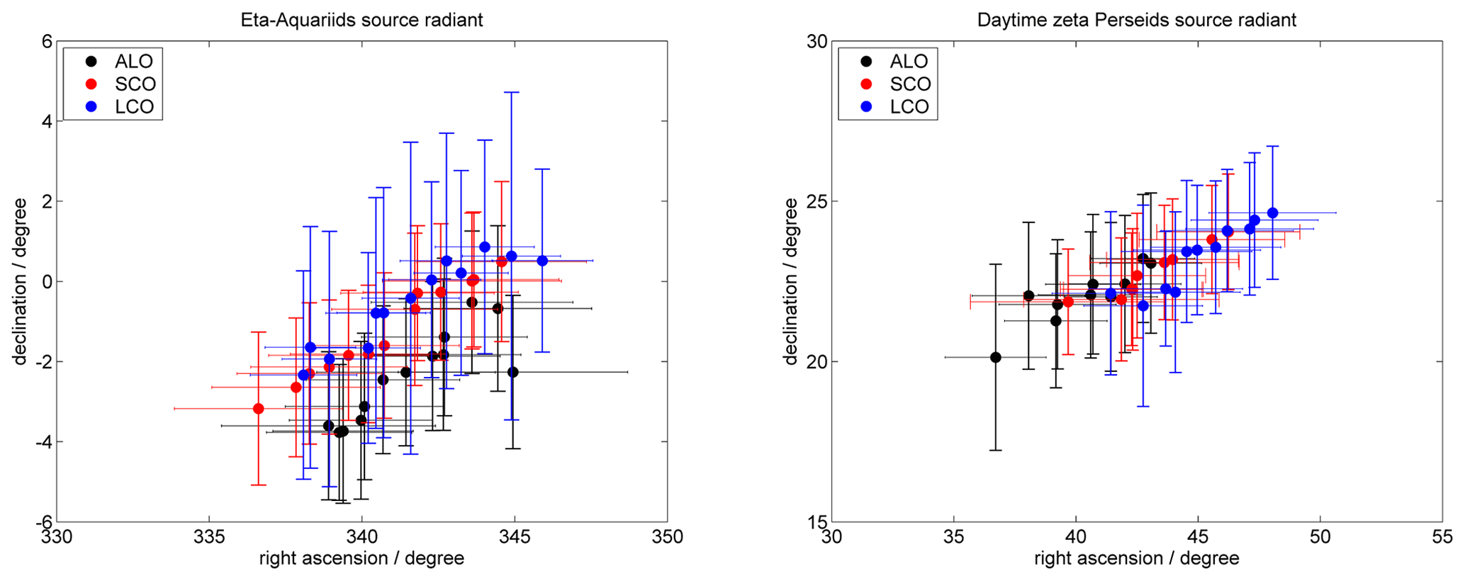
Figure B1 Scatter plots of meteor source radiant tracking for the eta Aquariids and daytime zeta Perseids.