Comparing airborne algorithms for greenhouse gas flux measurements over the Alberta oil sands

To combat global warming, Canada has committed to reducing greenhouse gases to be (GHGs) 40 %–45 % below 2005 emission levels by 2025. Monitoring emissions and deriving accurate inventories are essential to reaching these goals. Airborne methods can provide regional and area source measurements with small error if ideal conditions for sampling are met. In this study, two airborne mass-balance box-flight algorithms were compared to assess the extent of their agreement and their performance under various conditions. The Scientific Aviation's (SciAv) Gaussian algorithm and the Environment and Climate Change Canada's top-down emission rate retrieval algorithm (TERRA) were applied to data from five samples. Estimates were compared using standard procedures, by systematically testing other method fits, and by investigating the effects on the estimates when method assumptions were not met. Results indicate that in standard scenarios the SciAv and TERRA mass-balance box-flight methods produce similar estimates that agree (3 %–25 %) within algorithm uncertainties (4 %–34 %). Implementing a sample-specific surface extrapolation procedure for the SciAv algorithm may improve emission estimation. Algorithms disagreed when non-ideal conditions occurred (i.e., under non-stationary atmospheric conditions). Overall, the results provide confidence in the box-flight methods and indicate that emissions estimates are not overly sensitive to the choice of algorithm but demonstrate that fundamental algorithm assumptions should be assessed for each flight. Using a different method, the Airborne Visible InfraRed Imaging Spectrometer – Next Generation (AVIRIS-NG) independently mapped individual plumes with emissions 5 times larger than the source SciAv sampled three days later. The range in estimates highlights the utility of increased sampling to get a more complete understanding of the temporal variability of emissions and to identify emission sources within facilities. In addition, hourly on-site activity data would provide insight to the observed temporal variability in emissions and make a comparison to reported emissions more straightforward.

1 Introduction

Global warming is on the pathway to a minimal projected global temperature increase of 3.3–5.7 ^∘C by 2100 unless meaningful change is enacted to reduce anthropogenic greenhouse gas (GHG) emissions (Le Quéré et al., 2018; Friedlingstein et al., 2020; IPCC, 2021). Anthropogenic carbon dioxide (CO₂) and methane (CH₄) emissions are the first and second largest contributors to climate change, respectively (Friedlingstein et al., 2020). Accurate quantification of GHG emissions is an essential foundation for emissions reductions.

Regional, national, and global CH₄ and CO₂ emissions are estimated using a combination of bottom-up and top-down methods. In general, bottom-up methods aggregate and extrapolate source-specific data to estimate emissions at a larger scale, whereas top-down methods measure atmospheric GHG concentrations at a larger scale and infer point and area source emissions (National Academies of Sciences, Engineering, and Medicine, 2018). Anthropogenic CO₂ and CH₄ emissions are estimated using (a) ground-based methods, (b) airborne methods, or (c) satellite methods (e.g., Frankenberg et al., 2016; Conley et al., 2017; National Academies of Sciences, Engineering, and Medicine, 2018; Lauvaux et al., 2022; Irakulis-Loitxate et al., 2022). Large differences between bottom-up aggregated inventory estimates and top-down atmospheric budget estimates need to be reconciled to reduce the uncertainty in estimating global and regional GHG emissions (Nisbet and Weiss, 2010; Dlugokencky et al., 2011; Allen, 2014; Kort et al., 2014; Johnson et al., 2017; Alvarez et al., 2018; Liggio et al., 2019; Saunois et al., 2020; Friedlingstein et al., 2020; MacKay et al., 2021). Improved emissions estimates facilitate the best climate change policy (Le Quéré et al., 2018), allowing us to adopt pathways for lower global warming increases. This paper focuses on airborne approaches, as they are intermediate in spatial scale between proximal and satellite sampling methods and therefore improve estimation by providing essential validation between top-down and bottom-up methods (National Academies of Sciences, Engineering, and Medicine, 2018; Friedlingstein et al., 2020; Cusworth et al., 2020; Nisbet et al., 2020).

While some airborne methods utilize eddy covariance measurements (Yuan et al., 2015; Wolfe et al., 2018), methods for sampling anthropogenic GHG emissions using aircraft tend to fall into two major categories: (i) mass-balance methods (O'Shea et al., 2014; Gordon et al., 2015; Conley et al., 2017; France et al., 2021; Foulds et al., 2022) and ii) spectral imaging methods (Duren et al., 2019; Tyner and Johnson, 2021; Krautwurst et al., 2021; Cusworth et al., 2022). These methods capture atmospheric fluxes using varying approaches that are affected by different biases and are complementary when creating emission budgets. Mass-balance methods quantify the mass flux, or change, in the mixing ratio of a species due to emissions from a known source area. Sampling schemes for mass-balance flights range from flying a single transect downwind of a source, to multiple stacked transects creating a vertical “screen” to catch the plume at various altitudes, or flying a “box-flight” around a facility – or specific intra-facility source area – to constrain a plume (Gordon et al., 2015; Conley et al., 2017; Baray et al., 2018; Liggio et al., 2019; France et al., 2021). Remote spectral imaging methods fly above potential sources and use absorption spectroscopy of reflected solar radiance or thermal emissions to capture regional or facility emissions (Frankenberg et al., 2016; Bartholomew et al., 2017). Currently, mass-balance box-flight methods can attain a lower uncertainty from a single sample of emission estimates (∼2 %) (Gordon et al., 2015; Conley et al., 2017) than the spectral methods (<30 %) (Duren et al., 2019; Thorpe et al., 2020) due to smaller background and wind measurement uncertainties. However, they require an understanding of plume sources to know where to fly, and they can take longer; therefore they can be more costly.

Mass-balance box-flights involve sampling in stacked, often cylindrical, flight laps, typically surrounding a known source or set of sources, at altitudes varying from the minimum safe-flight altitude to the atmospheric boundary layer capping an emission plume (Gordon et al., 2015; Conley et al., 2017). Due to minimum flight height restrictions a gap between the surface and the flight box is inevitable. Concurrent surface sampling is ideal but often unavailable, so operators aim to fly at a distance from the source where the plume has risen enough but has not dispersed to the degree that it cannot be detected to capture the plume inside the box (Conley et al., 2017). For mass-balance box-flights, extrapolation to the ground is often the largest error source, nearing ∼30 % when the bottom of the plume is not captured (Gordon et al., 2015; Conley et al., 2017). Airborne mass-balance box-flight methods depend on the assumption of a stable boundary layer and that the emission plume is captured at the top of the box and does not change during sampling (i.e., that conditions are stationary) (Fathi et al., 2021).

Methods applying mass-balance equations to aircraft measurements have been developed and refined over the last two decades (Kalthoff et al., 2002; Alfieri et al., 2010; Karion et al., 2013; Gordon et al., 2015; Conley et al., 2017; Gordon et al., 2018; Krings et al., 2018; France et al., 2021). In this work, two box-flight mass-balance sampling methods, a top-down emission rate retrieval algorithm (TERRA) developed by Environment and Climate Change Canada (ECCC) (Gordon et al., 2015) and a Gaussian theorem algorithm developed by Scientific Aviation (SciAv) (Conley et al., 2017), provide two approaches to evaluate mass fluxes from aircraft measurements. To our knowledge, a detailed comparison of the two methods has not yet been conducted. If algorithm comparisons indicate agreement, then emissions estimates from multiple campaigns using mass-balance methods can be aggregated, which will improve the certainty in GHG budgets.

A complementary method to airborne mass-balance are airborne spectral methods, which can be considered top-down methods that produce results similar to satellite data but with higher accuracy (Kort et al., 2014; Frankenberg et al., 2016). Single flights are used to sample and estimate emissions from sources, and repeated sampling can determine source persistence to infer regional emission budgets (Duren et al., 2019). Stationarity of an emission plume occurs when the source of emission is consistent and meteorological conditions such as the boundary layer and wind are stable throughout the time of sampling. Remote spectral sampling provides quick “snapshots” of features and therefore avoids the stationarity requirement inherent to airborne mass-balance methods, which have lengthy sampling times ranging from less than one hour to multiple hours, depending on the region measured. Remote spectral imaging methods are being advanced by the NASA Jet-Propulsion Laboratory, which has had success in mapping, inferring wind vectors, and estimating emissions over large areas using their Airborne Visible InfraRed Imaging Spectrometer – Next Generation (AVIRIS-NG) (Frankenberg et al., 2016; Duren et al., 2019; Jongaramrungruang et al., 2019; Thorpe et al., 2020; Cusworth et al., 2021). Coincident sampling using the SciAv and AVIRIS-NG methods at facilities has indicated that the methods tend to agree, within errors (Duren et al., 2019; Thorpe et al., 2020).

Reducing GHG emissions in Canada has become a national and provincial priority (Johnson and Tyner, 2020; Government of Canada, 2021). Airborne and ground-based campaigns suggest that the inventories used to facilitate national and provincial policy are under-reporting GHG emissions (Brandt et al., 2014; Gordon et al., 2015; Johnson et al., 2017; Baray et al., 2018; Liggio et al., 2019; Chan et al., 2020; MacKay et al., 2021; Baray et al., 2021; Tyner and Johnson, 2021). For example, a recent study aggregated thousands of mobile, ground-based emission rate estimates taken without notice to operators from upstream Canadian oil and gas and found that inventories underestimated methane emissions (Atherton et al., 2017; MacKay et al., 2021). Using tower data, methane emissions estimates over 8 years from oil and gas operations in Western Canada were estimated to be nearly twice those reported in Canada's National Pollution Release Inventory (Chan et al., 2020). Airborne campaigns by ECCC measuring carbon dioxide and methane have also estimated emissions to be 13 %–123 % (Liggio et al., 2019) and 40 %–56 % higher (Baray et al., 2018), respectively, than national inventories. In a comparable campaign by Scientific Aviation, industrial upstream oil and gas CH₄ emissions estimated in two regions in Alberta were 5 and 17 times higher than values reported to the Alberta Energy Regulator (Johnson et al., 2017). Greater certainty in top-down emissions estimates helps flag under-reporting in bottom-up inventories and better informs GHG policy makers of emissions, allowing them to enact meaningful GHG reductions. As part of the Oil Sands Monitoring (OSM) program mandate to advance the understanding of Alberta's emissions, a collaborative study was initiated in 2017 by Alberta Environment and Parks (AEP) and the U.S. National Oceanic and Atmospheric Administration (NOAA), contracted to Scientific Aviation. The goal was to use airborne measurements to quantify facility- and activity-specific GHG emissions from mineable and in situ oil sands developments in northern and east-central Alberta. Between August 2017 and October 2018, sampling was conducted for various facilities and repeated over several days to assess both temporal and inter-facility variability in GHG emissions rates.

In this study, we compared emissions estimated using the same data from five box-flights from the 2017–2018 campaign using two airborne mass-balance algorithms (TERRA and SciAv). Our intention was to assess the comparability of emissions estimates from past campaigns flown by ECCC and SciAv, which may provide greater certainty of GHG emissions from the Alberta oil sands and other regions where these methods are used. The main objective was to test if emissions estimates from the TERRA and SciAv algorithms agreed with uncertainty and then to assess the sensitivity of emissions estimates to surface extrapolation using a variety of schemes. The cause of any differences between the algorithms was assessed. Since mass-balance flights are typically flown with the knowledge of and permission from facilities operators, these methods, while they may be accurate, may not necessarily reflect typical operating conditions or GHG emissions. Consequently, a secondary research objective was to examine the potential of utilizing complementary spectral imaging methods, such as AVIRIS-NG, to supplement mass-balance box-flights by providing contextual information to capture the spatial and temporal variability of oil sands GHG emissions.

2 Methodology

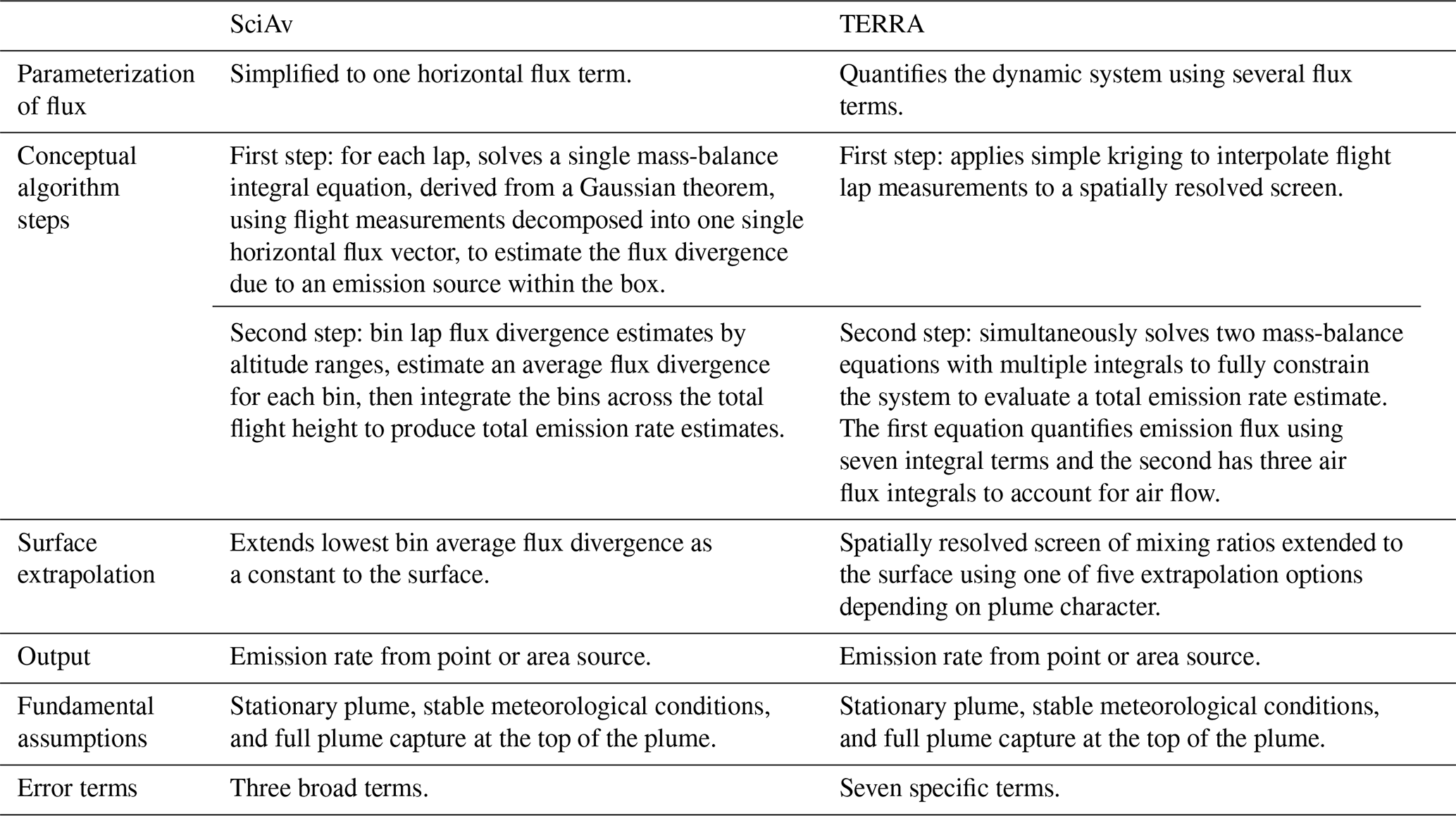
Both mass-balance methods involve flying around a known source in a box pattern to fully capture an emission plume for estimation, but they differ in their approaches (Table 1). TERRA evaluates the entire dynamic system with terms to quantify the horizontal advective and turbulent flux through the box walls and box top, deposition of flux to the ground, chemical mass changes, and air density changes (Gordon et al., 2015). TERRA applies a simple kriging of the raw data to spatially interpolate between the raw lap data, then estimates the dynamic terms to solve mass-balance equations and derive an overall total emission rate (Gordon et al., 2015). In contrast, the SciAv algorithm simplifies the system to a single horizontal flux through the box and estimates the flux divergence from the box by evaluating a mass-balance equation derived from Gauss's theorem for relating flux through a closed surface to a divergence from a volume integral (Conley et al., 2017). The SciAv and TERRA theory, including equations, are described in further detail in the Supplement – Sect. S1.1 and S1.2, respectively.

Table 1 Characteristics of the mass-balance SciAv and TERRA algorithm for box-flights.

2.1 Box-flight aircraft measurements

The AEP-NOAA-Scientific Aviation 2017–2018 Alberta oil sands flight campaign conducted 150 flight segments at 16 different facilities across Alberta. Many of these facilities included multiple source areas, such as a plant, a mine, and/or tailings ponds. The aircrafts flew in laps around either the entire perimeter of a facility or around specific source areas. The data were collected and processed by Scientific Aviation (Boulder, CO, USA) on contract to NOAA. Flights were performed using two fixed-wing, single-engine aircraft, a Mooney M20R (Aircraft N617DH) and a Mooney M20M (Aircraft N2132X), equipped with monitoring equipment. Concentrations of CO₂ and CH₄ were measured using a cavity ring-down spectrometer (Picarro 2401m or 2210m, Picarro Inc., Sunnyvale, CA, USA) in its precision mode at ∼0.5 Hz, as described by Crosson (2008). Other variables used in the analysis were measured using the airplane primary flight information system and GPS, including wind speed components (m s⁻¹), pressure (mb), temperature (K), heading (degree), altitude (m), and latitude and longitude. Each flight segment was screened to assess whether (i) sufficient altitude was reached to capture the entire plume, (ii) winds were sufficiently strong and consistent, and (iii) upwind sources were negligible relative to emissions inside the box. If these criteria were not met, then the algorithm results (i.e., emissions estimates) were considered unreliable. It was challenging to determine a quantitative threshold for adequate wind conditions or negligible upwind sources, since the relative impact on the calculated emission rate depends on the magnitude of emissions. Nonetheless, any flight segments with average wind speeds below 5 m s⁻¹ were flagged (Gordon et al., 2015), as were flight segments with upwind mixing ratios above background, and were then assessed further using professional judgement. It is important to note that light and/or variable winds will increase the uncertainty of the SciAv algorithm by increasing the variability between laps.

Five flights from three facilities were selected for the algorithm comparison and are summarized in Table 2, with sample codes (F01 to F05) assigned for comparison purposes. The three facilities from the Athabasca oil sands region included in the study were: Mildred Lake and Aurora North plant sites (Syncrude), Horizon Oil Sands Processing Plant and Mine (CNRL), and Suncor Energy Inc. oil sands (Suncor). Flight paths around the facilities are shown in Fig. 1. These five flights were chosen to capture a range of possible sample types given varying profile shapes, number of laps, boundary layer height, season, and whether the flight was around a facility perimeter or plant. Four of the five flights selected were considered ideal samples during preliminary flight screening. One flight, F05, was chosen as a poor-quality sample, rejected during flight screening as having “not fully captured” the top of the emission plume, and used to assess how the methods compare when a fundamental assumption of the method is not met. Boundary layer height was estimated by Scientific Aviation by assessing profile changes in potential temperature gradients before and after flights. Through the flight screening process, all five flights were judged to have consistent, stationary winds and stable boundary layers. F02 had normal operating conditions and no flaring events reported by CNRL Horizon. Facilities were informed before sampling. Operating conditions at the oil sands facilities for F01, F03, F04, and F05 were not shared at the time of writing.

Table 2 Information on the five box-flight samples used in the comparative analysis.

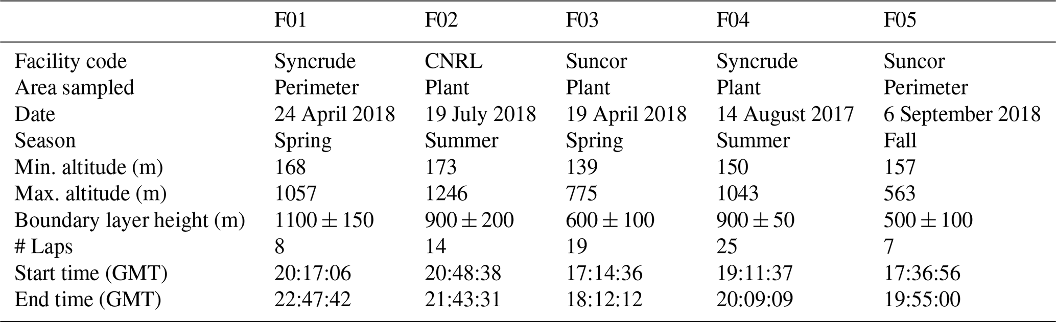
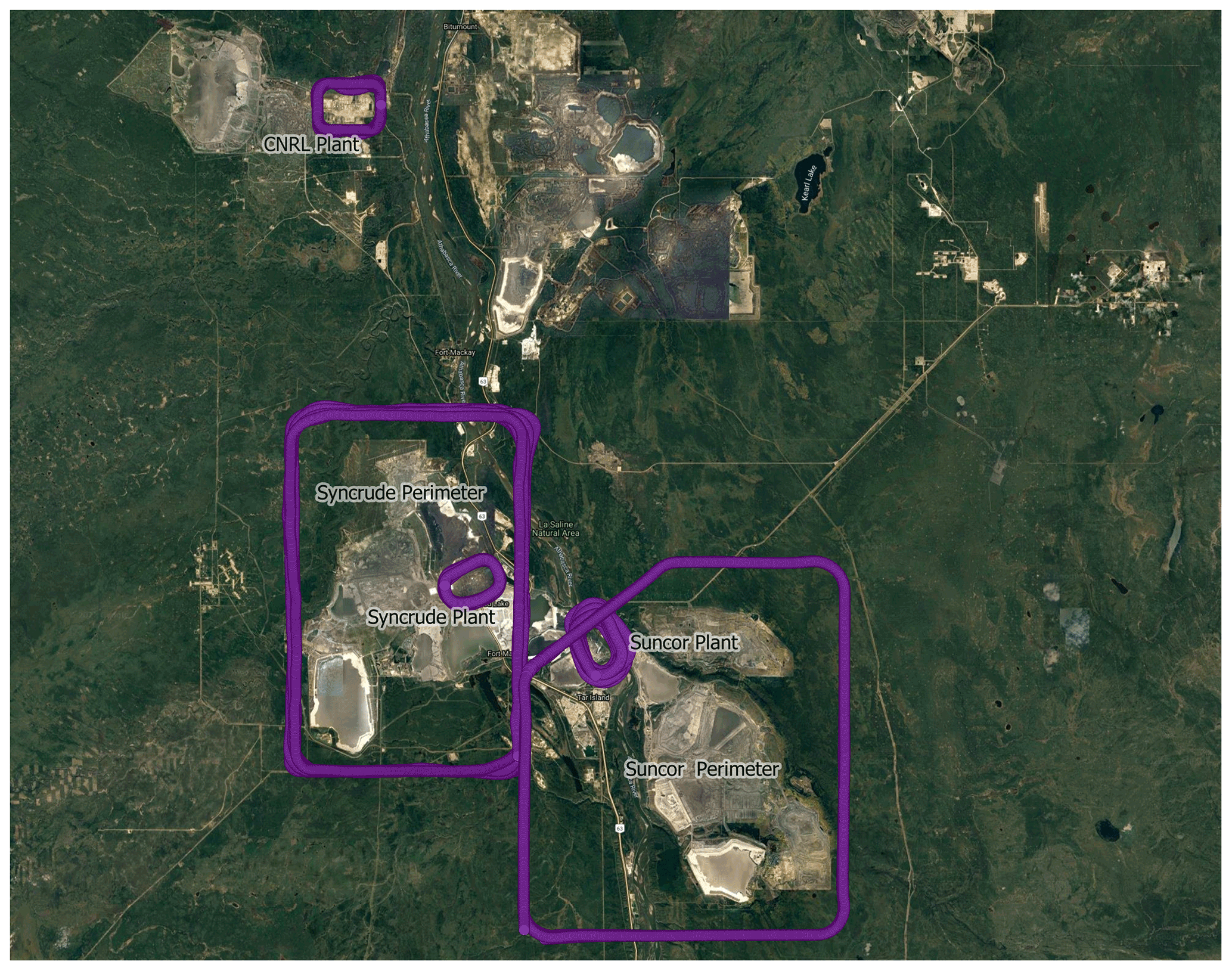
Figure 1 The flight paths (one second intervals) are shown for each facility sample used in the study. Perimeter flights are the large polygons, and plant flights the smaller ovals. Map layer data © Google Satellite Hybrid 2017.

Figure 2 shows an example of a close view of a flight path for F04 CH₄. Blue dots indicate background levels in ppm, and enhanced mixing ratios within the plume are in a gradient of cyan-yellow-red, with the largest enhancements in red. A large plume can be seen on the north-east section of the flight path in Fig. 2, and a few enhancements were measured elsewhere along the flight path. There is evidence that the top of the plume is captured, as dots at the highest altitude show background concentrations, and the flight path goes above the estimated boundary layer.

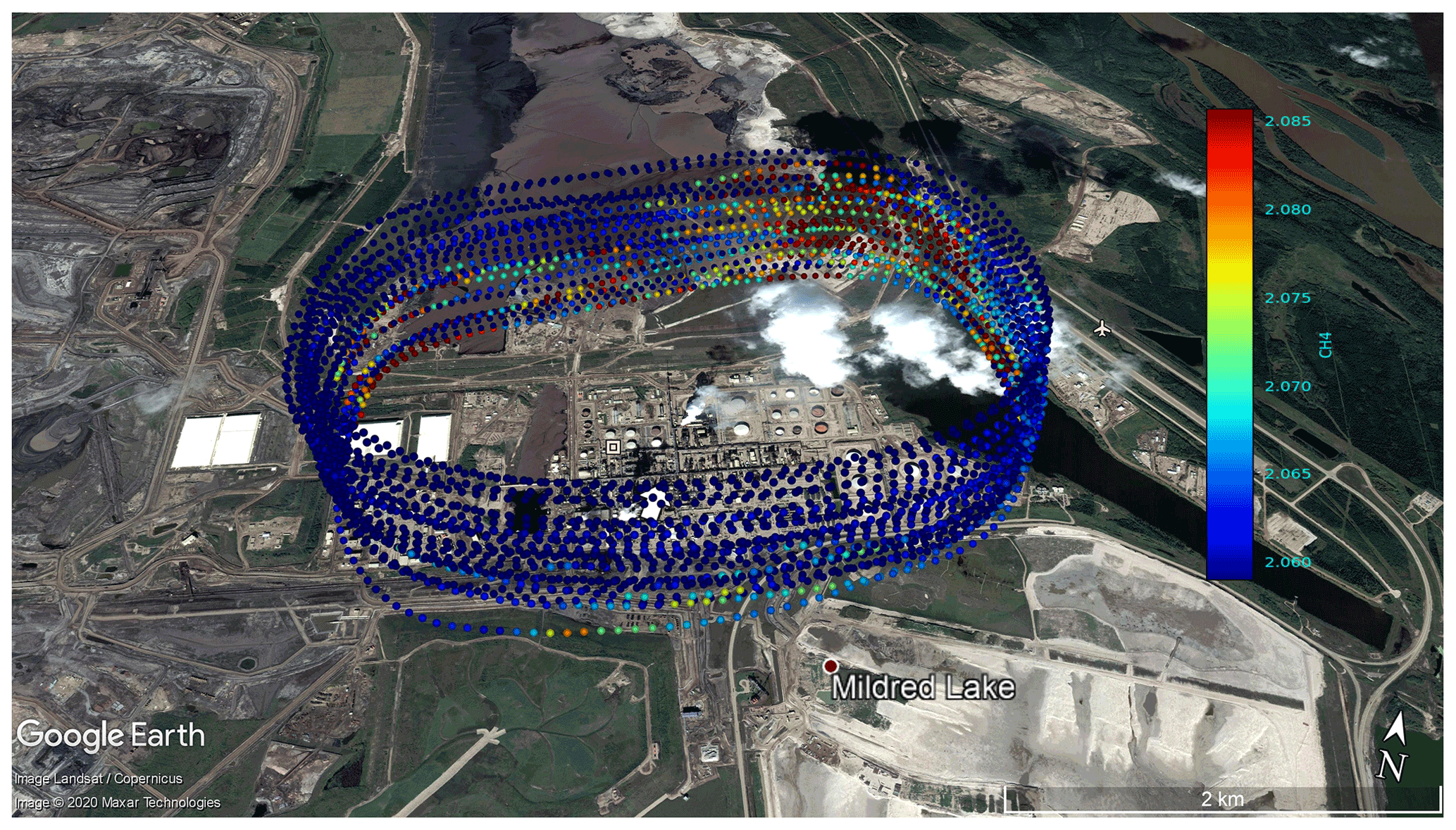
Figure 2 The flight path for F04 depicts the mixing ratio of CH₄ (ppm) measured at 1 Hz intervals for each of the 25 laps around the Syncrude plant. A Google Earth historical image from September 2016 was used, as it shows an emission plume with wind conditions similar to the 2017 F04 flight. A KML file containing mixing ratios provided by Scientific Aviation was overlaid on the image. Each measurement of a mixing ratio is depicted as a dot, and the layout traces the 25-lap flight path for sampling during F04. Satellite imagery © 2020 Maxar Technologies, Google Earth.

2.2 Box-flight emissions estimate algorithms

2.2.1 TERRA algorithm

Environment and Climate Change Canada (ECCC) provided the TERRA algorithm, ran portions of the analysis, and detailed instructions on how to produce estimates using the algorithm with commercial plotting software (IGOR Pro 8, Wavemetrics, Lake Oswego, OR, USA). The first step of the TERRA algorithm creates the screen of spatially interpolated lap data by applying simple kriging to the campaign data collected by Scientific Aviation. The spatially resolved screen of mixing ratios is a 2-dimensional unraveling of the lap data by altitude over the length of sampling and is commonly referred to as the “box” (Gordon et al., 2015).

For the second step, TERRA has 5 options for extrapolating emission concentrations from the lowest flight layer to the surface to account for fluxes below the flight path: (1) a background extrapolation fills all data below the flight path with a background concentration (applied when there is a fully captured, elevated plume and there is a reason for choosing one single mixing ratio to be extrapolated to the surface); (2) a constant extrapolation uses the concentration at the bottom of the screen and assumes that this remains constant to the surface (best used in the general case of a fully captured, elevated plume, as it avoids the assumption of a background value); (3) the linear method fits a line through the lowest points on the screen up to an altitude of 300 m above ground level (preferred in the scenarios when emissions occur from the surface, such as a low plume that was not fully captured or a mixed plume with ground sources such as a tailings pond); (4) the interpolation between the concentration at the lowest altitude of the screen and the background concentration at the surface (ideally used when there is evidence of decreasing emissions with only a trace of the plume at the bottom of the flight path); and (5) exponential extrapolation calculates a Gaussian fit through the lowest points on the screen (largely avoided unless there is a strong argument that it best fits the plume behaviour).

Surface extrapolation was essential for this study, as all flights had emission plumes that were not fully captured at the lowest flight track. For the TERRA standard estimates, a linear fit was used for F01, F03, and F05 for both CH₄ and CO₂ due to their low position on the screen and their likelihood of having an increasing emission towards the surface. An interpolation to background fit (i.e., Option 4 described in the paragraph above) was applied to F02 for both CH₄ and CO₂, and F04 for CO₂, as these cases largely captured plumes with low mixing ratios at the bottom of the flight path. A constant extrapolation (Option 2) was fit to F04 for CH₄ to avoid an assumption about the background concentration, as it was the one flight with a very large plume dispersion where plume behaviour was unknown (Sect. S1.3). All extrapolation outcomes were produced to calculate the surface extrapolation error, which accounts for potential differences when choosing the best surface extrapolation (Gordon et al., 2015), and to compare it with the range of possible outcomes from the SciAv method by running a bootstrap analysis. The settings for the standard TERRA emissions estimate were chosen by assessing the plume location, boundary layer conditions, and plume source information to determine the appropriate surface extrapolation (Gordon et al., 2015; Baray et al., 2018).

The TERRA total uncertainty estimate was calculated by adding seven error terms in quadrature (i.e., by taking the square root of the sum of squares). Four of the seven TERRA error terms were evaluated. The wind and measurement error had been previously determined to each be <1 %, and the vertical turbulence term had been functionally removed from TERRA analysis (Gordon et al., 2015; Baray et al., 2018). The surface extrapolation error was calculated as the maximum percent change amongst the plausible surface extrapolation estimates. For example, background extrapolations (Option 1), which assume no mixing ratio enhancement below the flight path, were not considered for standard estimates when a flight had increasing emissions at the bottom of the screen. A description of the calculation of the box-top mixing ratio, air density, and box-top height error terms is given in Sect. S1.4.

2.2.2 SciAv algorithm

Scientific Aviation provided results from the first step of estimating the flux divergence for each lap. They applied their algorithm to the flight data and provided output that could be used to address the research objectives. Although the algorithm itself is proprietary, the concepts and formulae underpinning the algorithm are described in detail in Conley et al. (2017). The algorithm output included standard emissions estimates and uncertainties using the SciAv preferred settings. It also included profiles of flux divergence and uncertainty for each lap versus altitude and preferred bin altitude ranges. These were used in the second step analysis of binning lap estimates and integration of the flight profiles to test cases such as extrapolation to the surface in MATLAB 2020a (The MathWorks, Inc., Natick, Massachusetts, United States). Figure 3 provides an example profile of the average flux divergence per lap estimate calculated in the first step of the SciAv algorithm. A flight is classified as “fully capturing” the emission plume when the mean flux divergence of the highest flight laps approaches zero. The standard SciAv emissions estimates assume that the flux divergence profile is constant below the lower flight altitude.

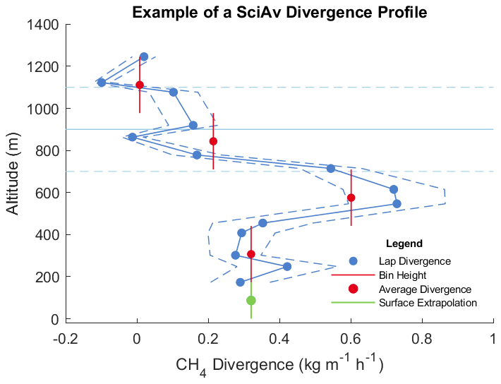
Figure 3 An example of a SciAv profile used in the second step of the method. The blue points are the estimated flux divergence for each lap, which are connected to show profile shape with the associated uncertainty (a dashed blue line). Red points are bin averages, and the vertical red bar is the bin height range. The boundary layer height is drawn in light blue with error bars (light blue dashed lines). The standard SciAv surface extrapolation method of extending the lowest red bin to the surface is shown in green.

For this study, the use of different surface extrapolations for SciAv were developed and tested. To obtain a greater range of possible outputs from the algorithm, SciAv was fit using differing surface extrapolation methods: (1) constant (SciAv's standard of extending the lowest bin to the surface); (2) background (estimating flux divergence as zero by applying no extrapolation below the lowest profile point); (3) linear (estimating the linear trend of the profile points at a specific height that was chosen given the profile shape, location of the plume enhancement, and sparsity of points, and extrapolating the trend to the surface); (4) linear weighted (estimating the linear trend of the profile points, but weighted by the calculated flux divergence uncertainty for each lap estimate); (5) linear interpolation to background (fitting a line between the lowest profile bin), and (6) the average of the surface points calculated in methods (1)–(5) (Sect. S1.5).

The data used for both the TERRA and SciAv methods were identical, but due to different approaches to assessing conditions and analysis of the data, different error estimates were produced. Conley et al. (2017) found that binning by lap and using a constant extrapolation produces a stable estimate when 20–25 laps are flown around an emission source (Conley et al., 2017). However, with larger area samples, such as perimeter flights, fewer than 10 laps are often flown. These types of samples may be better suited to a different type of integration as well as surface extrapolation. A potential method of improving estimation in the SciAv methods was investigated by using trapezoidal integration rather than binning to estimate a total emission estimate from the lap flux divergence points. Figure 4 depicts the two methods of integrating the SciAv flux divergence profiles as well as the different types of SciAv surface extrapolations, using the profile for F01 CH₄ as an example. The same surface extrapolation estimation procedure was used for both the binning and trapezoidal methods (Sect. S1.7). Surface extrapolation methods were fit to the lowest flux divergence lap point for the trapezoidal method to remain consistent with the SciAv method.

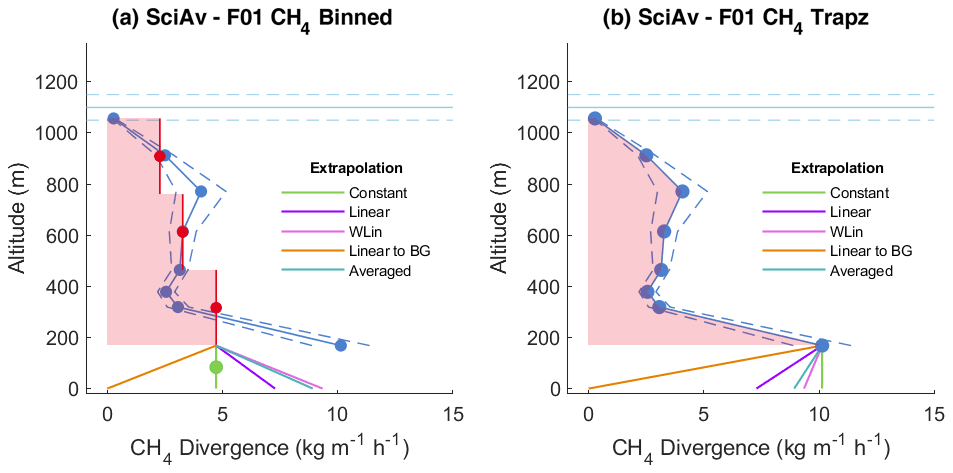
Figure 4 The two different integration methods applied to the SciAv F01 CH4 profile are depicted as the red area. Figure (a) shows the standard binning method of estimating an average flux divergence for each bin and integrating by altitude over the area as rectangular boxes. Figure (b) shows the trapezoidal (Trapz) method of estimating an average area under the curve by connecting the flux divergence lap points. The boundary layer height is drawn in light blue with error bars (light blue dashed lines). Both figures do not include the extra emissions that would be included using surface extrapolation.

2.3 AVIRIS-NG aircraft emissions estimates

Three days prior to the F04 flight, a NASA Jet Propulsion Laboratory (JPL) AVIRIS-NG flight covered the Syncrude plant. This measurement was part of a larger Arctic-Boreal Vulnerability Experiment (ABoVE), which included flight lines flown over the Alberta oil sands region. AVIRIS-NG measures ground-reflected solar radiation (380–2500 nm) with a 34^∘ field of view and a spectral resolution of 5 nm to map CH₄ plumes by utilizing absorption features in the shortwave infrared (Thorpe et al., 2017, 2020). As described in Duren et al. (2019), emissions estimates are calculated by combining the integrated mass enhancement (IME) and wind speed, as demonstrated in a number of recent studies throughout the United States (Cusworth et al., 2021, 2022) as well as a controlled release experiment (Thorpe et al., 2021). Previous studies have shown that the AVIRIS-based estimates of methane emissions agree well with box-flight emissions (Frankenberg et al., 2016; Duren et al., 2019; Thorpe et al., 2020). Figure 5 shows the AVIRIS-NG plume imagery that was captured over the Syncrude plant site with the Scientific Aviation KML lap data (shown in Fig. 2) overlaid. By measuring emissions at the same facility within a few days, this independent sample using a different method provides a contrast to the box-flight, mass-balance data.

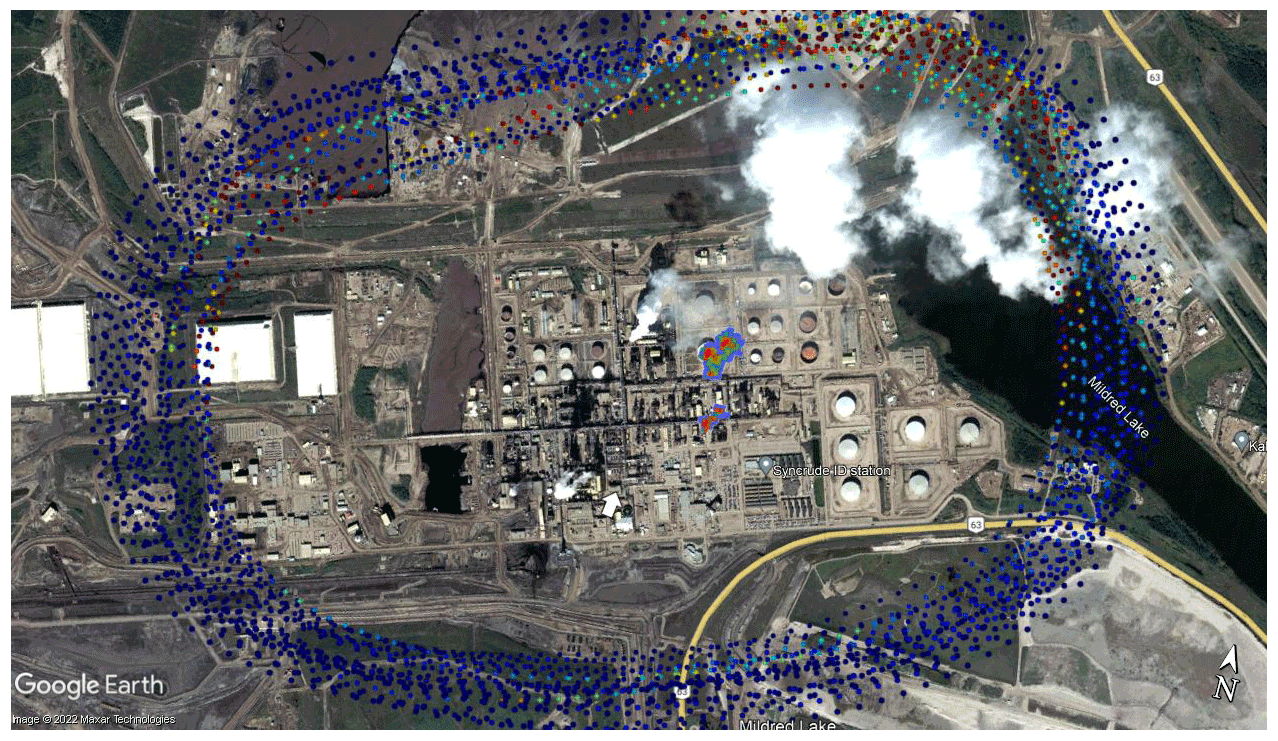
Figure 5 AVIRIS-NG-captured CH₄ column enhancements are shown from 11 August 2017 inside the F04 raw CH₄ lap data around the Syncrude plant from SciAv for 14 August 2017 using the Google Earth historical image from September 2016. AVIRIS-NG data and imagery provided by the NASA-JPL and satellite imagery © 2020 Maxar Technologies, Google Earth. Large CH₄ enhancements are depicted in red. The wind direction is shown by the white arrow, as measured by SciAv.

AVIRIS-NG data were collected at 5.3 km (17.5 kft), and the Syncrude facility was not informed prior to sampling. NASA-JPL provided CH₄ emissions calculated using AVIRIS-NG data and three sources for hourly estimation of the wind: ECCC meteorological towers 3062696 and 3062697, and MERRA2 (Modern-Era Retrospective analysis for Research and Applications, version 2) reanalysis. MERRA2 is an atmospheric reanalysis method produced by NASA that utilizes numerous satellite observations to produce a global time series of atmospheric data (Gelaro et al., 2017). To estimate variability in wind speed, an average over a 3 h window was used for the met tower data, and nine kernels centred on the plume latitude and longitude were used for the MERRA2 analysis. The magnitude of the AVIRIS-NG estimates was then compared to the SciAv estimate as an independent way of evaluating the temporal consistency of emissions.

3 Results

3.1 Box-flight emissions estimate comparisons

Standard Scientific Aviation (SciAv) emission results were compared to the estimates produced by applying TERRA to the same flight data. A constant extrapolation to the surface was used for all SciAv samples, whereas the extrapolation for TERRA varied by the flight profile and source. The standard estimate results from both algorithms are shown in Table 3 and Fig. 6. RStudio (RStudio Team, PBC, Boston, Massachusetts, United States) was used for comparison analysis, and comparison figures were created using the ggplot2 package (Wickham, 2016). Standard emissions estimates for four of the five flights agree within their uncertainties. Confidence intervals for the estimates were not produced, as there is only one estimate for each flight, and therefore the error bars are simply the range for each estimate. In Fig. 6, the error bars for each estimate overlap with each other, aside from F04, which has a large gap between estimates. The uncertainty for the TERRA estimates are consistently smaller than for SciAv (averaging ∼8 % smaller).

Table 3 Results of the CH₄ (in kilograms per hour) and CO₂ (in tonnes per hour) standard fit estimates from each algorithm, with their uncertainty as a percentage ± % and the range derived from the percentage uncertainty of each standard estimate.

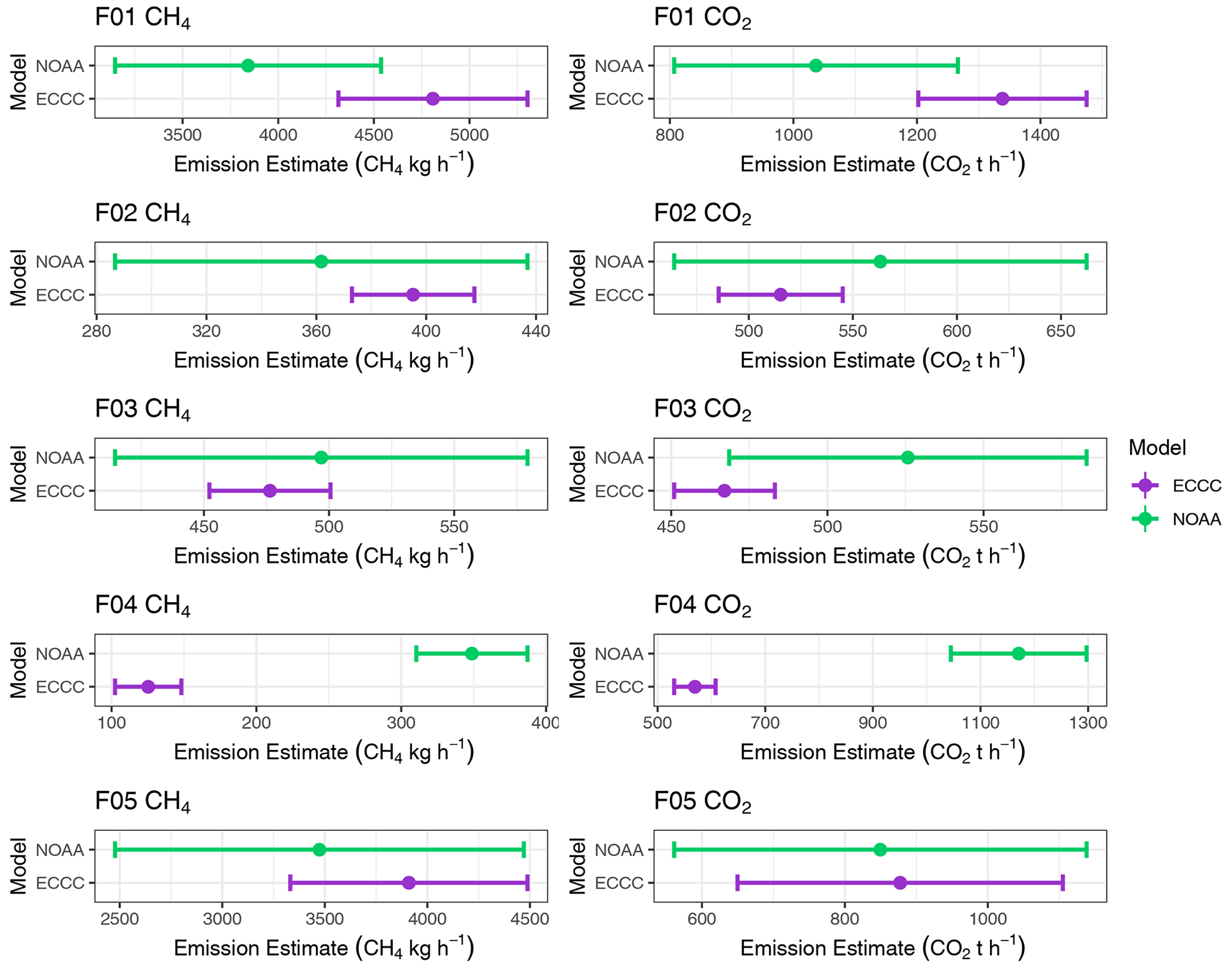
Figure 6 Flight emission estimates for CH₄ (left) and CO₂ (right) derived for each algorithm are plotted as points, along with the range of each estimate, as error bars. TERRA standard estimates are shown in green and SciAv in purple. Samples of F01, F02, F03, and F05 produce estimates that coincide within each method's error bars.

Algorithm agreement is implied when the range for each estimate overlaps. For all flights except F04, the differences between the algorithms are in the range of the estimate uncertainties. For F04 the emissions estimates disagreed, as there is a large gap between the estimates with no overlap of the ranges. To compare the estimates using the uncertainty range, the relative mean percentage difference and propagated percentage uncertainty of the two estimates were calculated. The whole set of results from five flights was formally tested for differences between the SciAv and TERRA estimates using a weighted t test and Wilcoxon signed rank test. As a collective, the differences between the algorithms were found to be insignificant for both CH₄ and CO₂ (Sect. S1.6).

Large, anomalous differences between the SciAv and TERRA estimates occurred for F04. During screening of the flights, no issues with F04 were flagged (Sect. S1.8). This flight can be used as an example for improving SciAv flight screening and for assessing the implications when assumptions of a stationary plume and stable meteorological conditions are violated. No other flights had non-stationary conditions. The flight that was intentionally included as a poor-quality sample (F05), due to the large emission plume occurring at the highest altitude transects flown, has very good agreement between the two algorithms.

During the study design, F04 was considered an ideal sample, and the non-stationarity of the emission plume was not flagged until more in-depth analysis was applied to discern the reason for the large disagreement between the two algorithms. Over the course of F04, the concentrations of CH₄ and CO₂ changed, both within the plume (downwind of the plant) as well as in background air masses (upwind of the plant). Based on available information, it is unknown whether changes in facility emissions contributed to the observed changes in the plume's non-stationarity. It was noted that during sampling, facility operators instructed researchers that future flights could only sample the boundary of the facility. Operating conditions were not provided by the industry. NO₂ and SO₂ emissions are often used as tracer data for upscaling CH₄ emissions (Baray et al., 2018; Li et al., 2017; Liggio et al., 2019). Continuous emissions monitoring system (CEMS) facility stack emissions during F04 were consistent with typical operations and showed that NO₂ emissions spiked at the beginning of the day, before the aircraft measurements, and then continuously decreased. Furthermore, flaring data, including the volume of gas flared and SO₂ emissions, did not suggest unusual operations at the plant on the day of the flight. The disagreement between the two algorithm estimates for F04 arise from the non-stationary emission plume, which affected the box-flight mass-balance algorithms.

To test the effect of assumptions associated with plume shape below the lowest flight lap, various surface extrapolations were applied to the lowest bin of the SciAv flux divergence profiles for all five flights. The set of all results, based on the differing surface extrapolations, was compiled (Sect. S1.3 and S1.5), and estimates are plotted together in Fig. 7. Estimates that clustered together for both methods indicate a good agreement, with little difference between the varying surface extrapolation estimates. F04 has large disagreement between algorithms for both CH₄ and CO₂ (Fig. 7). The mean emission estimate and standard deviation of each method's various surface extrapolations were calculated (Sect. S1.6). The larger the spread in estimates, the more sensitive the flight was to the choice in extrapolation. Systematic bias is not evident in the differences between algorithms, as emissions estimates intersect, and no one method produces consistently larger or smaller estimates for all flights. To remove the effect of the choice in surface extrapolation, estimates were produced by background mixing ratios below the lowest flight path. These estimates were compared, and the SciAv and TERRA methods were still found to agree (Sect. S1.6).

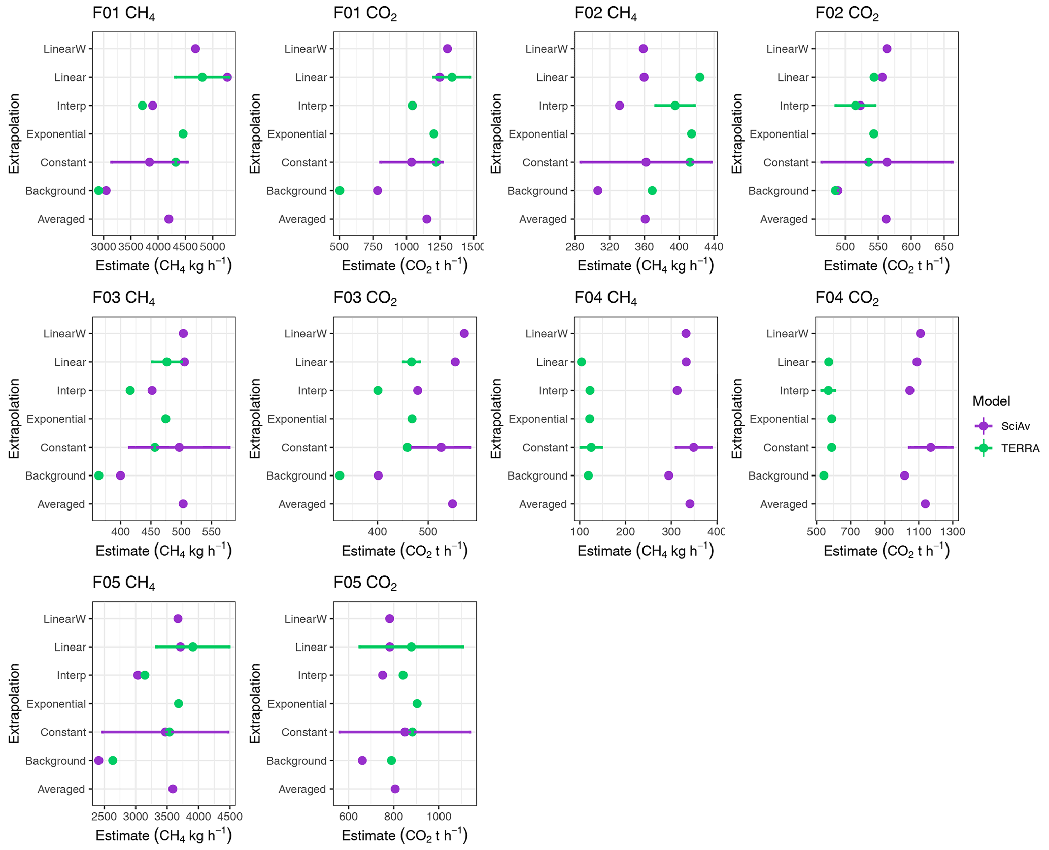
Figure 7 CH₄ and CO₂ estimates, based on various surface extrapolation fits, are plotted in purple for the SciAv estimate and green for TERRA. Error bars are drawn onto each algorithm's standard estimate.

To assess the sensitivity of emissions estimates using different surface extrapolations, the differences between each algorithm were calculated for the same four surface extrapolations (Sect. S1.6). For most flights, the choice in surface extrapolation had only a small effect on the difference between the estimates (≤3 %). The choice in surface extrapolation is a source of large variation between the algorithms for F01, the one flight with large emissions at the lowest flight path. The average of the estimates using the same four surface extrapolations was also computed. There is no evidence that agreement changes when removing the effect of surface extrapolation, and there is consistent agreement between the algorithm estimates (Sect. S1.6).

For each flight, algorithm estimates for the whole set of varying surface extrapolations were resampled using the bootstrap method (described below) to estimate the range in the difference between estimates based on the various surface extrapolations for each flight. The difference between the two algorithms, based on the various surface extrapolation estimates, was computed and contrasted with the standard error of each estimate. In Fig. 8, the distribution of the randomly sampled mean difference was calculated using the bootstrap method and plotted along with the propagated uncertainty range for each flight and gas (CH₄ and CO₂). A value of zero implies that there is no difference between the methods. Aside from F04, the distributions all either include zero, or the uncertainty of the standard estimates include zero, indicating that there is good agreement between the algorithms in most cases.

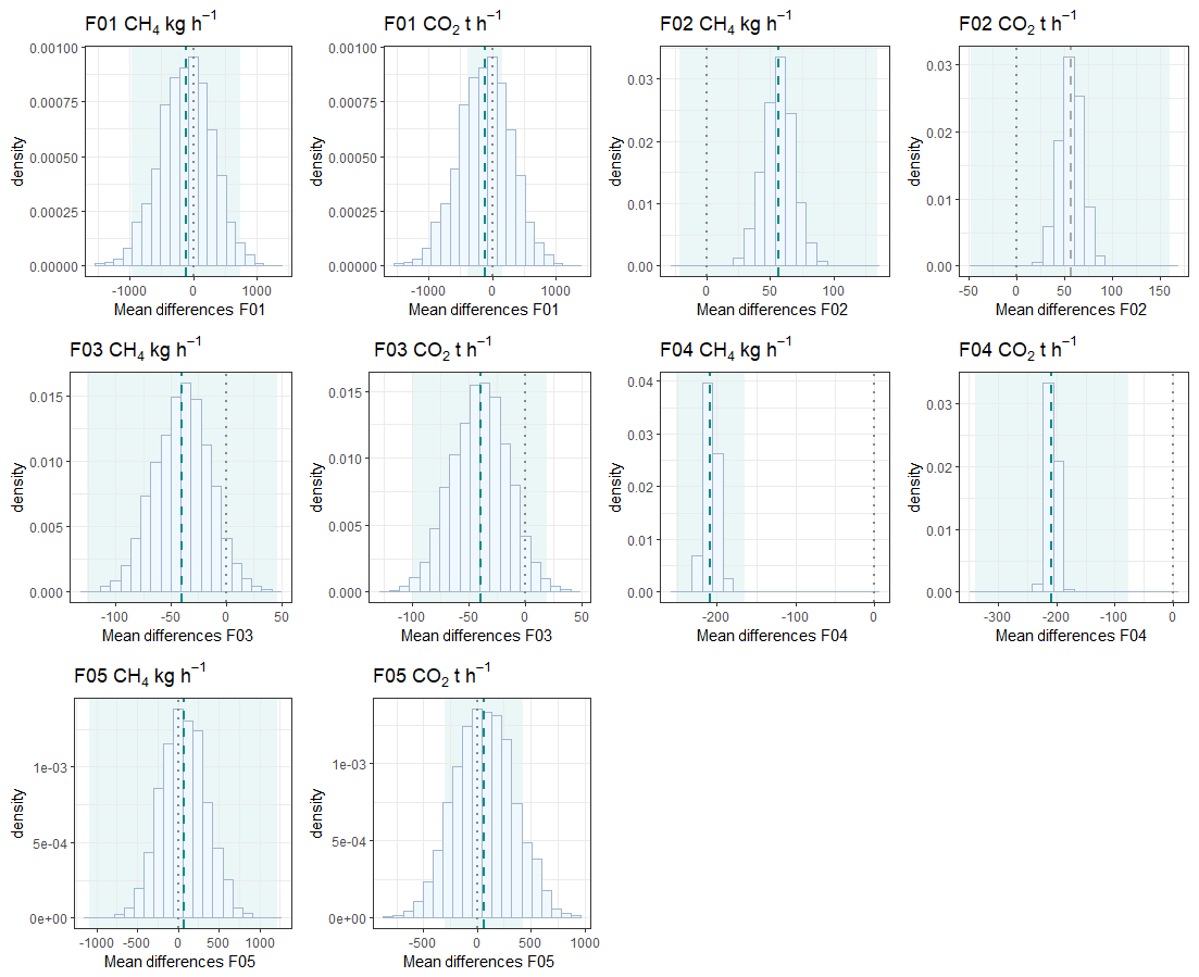
Figure 8 Distributions of the mean difference between all fits of CH₄ and CO₂ for the SciAv and TERRA algorithms are shown as a light blue histogram. The mean difference between the standard estimates is plotted as a teal dashed lined, and the range in the difference between standard estimates is shown as a light teal box. A grey dot dashed line is drawn at zero as a reference point for the location of exact agreement between the algorithms.

3.2 AVIRIS-NG aircraft emissions estimates

CH₄ enhancements were imaged at the Syncrude plant site within the perimeter of the Scientific Aviation box-flight path of F04 at 21:17:24 UTC on 11 August 2017 (Fig. 9), 3 d prior to the SciAv flight. There appeared to be two separate source plumes on that day, both of which were well inside the mass balance transects flown by Scientific Aviation during F04. The F04 flight also appeared to capture these two plumes (see Fig. S9). NASA-JPL provided data, analysis, and plume imagery using the methods described in Duren et al. (2019) over the F04 site to help provide additional context for the aircraft measurements (Table 4). The average instantaneous CH₄ emission rate of estimates derived using three different wind speed and direction datasets was 1665 (kg h⁻¹), with an average uncertainty of 707 (kg h⁻¹). This average emission rate likely reflects day-to-day emissions variability, as it was approximately 5 times larger than emissions measured using the SciAv method 3 d later (349 kg h⁻¹). However, the AVIRIS-NG-derived emission rate was significantly less than the SciAv Syncrude perimeter estimate (F01, 3840 kg h⁻¹ and F05, 3470 kg h⁻¹).

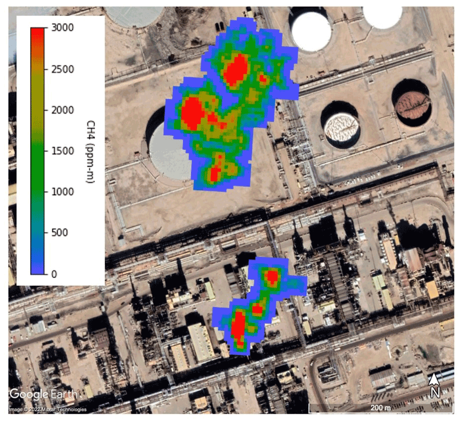
Figure 9 AVIRIS-NG observed CH₄ enhancements were imaged at the Syncrude plant site on 21:17:24 UTC. There appear to be two distinct sources located in close proximity. Satellite imagery © 2020 Maxar Technologies, Google Earth.

Table 4 AVIRIS-NG data captured on 14 August 2017, 3 d prior to the F04 flight, is estimated using three sources of wind data.

4 Discussion

4.1 Box-flight emissions estimate comparisons

In general, when fundamental assumptions were met, the SciAv and TERRA algorithms produced similar results. For the average flight scenario, the algorithm estimates derived using various surface extrapolations tended to agree regardless of how the surface extrapolation was fit. This consistency between estimates provides larger certainty in the estimates and in the top-down regional budgets that are inferred from them and also implies that emissions estimates between studies using different algorithms can be compared.

The SciAv and TERRA estimates were also compared when no surface extrapolation was applied (the background surface extrapolation scenario). These estimates also agreed, which suggests that the first steps in the core mass-balance algorithm produce similar outputs. Results from applying multiple surface extrapolations indicate that a potential difference between the methods may occur in the second algorithm step, due to the different methods of extrapolating to the surface, when an emission plume increases towards the surface.

Plots of the SciAv lap flux divergence estimates tend to follow three profile types. Examples of the three profile types for measured CH₄ lap enhancements (with uncertainties), as shown in Fig. 10, are (1) an emission plume with constant enhancements persisting at the lowest flight track (type I); (2) an elevated emission plume where enhancements approach zero at lower altitudes (type II); and (3) a plume that has enhancements increasing towards the surface (type III). All the profiles shown in Fig. 10 fully capture the top of each emission plume. Of the five sample flights compared, three had clear profile shapes. The SciAv method of extrapolating as a constant is the most appropriate choice unless a type III pattern of increasing emissions at the lowest flight path is evident.

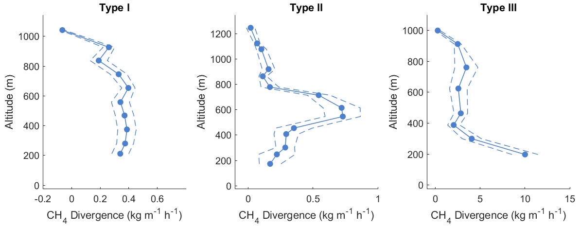
Figure 10 Sample data representing the three common types of flux divergence profiles for the SciAv method. Blue dots represent the flux divergence of each lap, with the associated uncertainty drawn as blue dashes.

F01 was the only flight with a definitive SciAv profile type III and highlights the difference in the approaches to surface extrapolation when emissions increase at the lowest flight track. An “increasing-to-surface” fit for profile type III shapes would likely improve estimate accuracy for the SciAv algorithm. SciAv fits a constant surface extrapolation regardless of the behaviour of emissions at the lowest flight path, whereas TERRA chooses the surface extrapolation from various fits by assessing the plume. When a flight has large emissions at the bottom of the plume, the SciAv and TERRA methods agree more when some form of increasing-to-surface extrapolation is applied to SciAv compared to the use of the standard, constant extrapolation. This indicates that the second step of each algorithm, the choice of an appropriate surface extrapolation, is likely a significant factor contributing to any differences between the methods for type III profiles (see Fig. 10).

For the five flights compared, the uncertainty from TERRA is lower than that from the SciAv by an average of 8 %. The smaller uncertainty for the TERRA estimates may be due to how each algorithm quantifies error. TERRA calculates seven specific error terms to address the error of these assumptions. Increases in the error of one assumption do not directly increase the error of others (see Sect. S1.4). On the other hand, SciAv uses two main broad terms: a temporal error term to capture the extent of stationarity and a flux divergence error term to estimate capture of the plume. The flux divergence error of SciAv can become very large when only a few flight laps are flown. The uncertainty in the surface extrapolation from the SciAv algorithm may be reduced if it is decoupled from the current flux divergence error term and calculated following TERRA methods (i.e., using the maximum percentage change between probable fits).

The mean of the estimates derived using the six different surface extrapolations were calculated for each integration method's set of results, and differences were tested using a pairwise t test and Wilcoxon signed rank test. There was no evidence of a difference in mean estimates for each flight between the two integration methods evaluated (binning vs. trapezoidal; Sect. S1.7). This indicates that, for this adaption of the SciAv algorithm, choosing a different surface extrapolation is more important than the type of integration method. To further assess the effects of applying different surface extrapolation options, surface measurements at the time of sampling and more information about the behaviour of a plume are the most likely path towards further reducing the uncertainty for both algorithms.

4.2 Box-flight algorithm assumptions investigated

During the initial screening of F04 by members of Scientific Aviation and AEP, the non-stationary plume was not identified, as focus was placed on assessing meteorological conditions and plume capture. Meteorological conditions are often the most likely source of non-stationarity; as such both SciAv and TERRA methods apply a set of criteria to screen samples. TERRA also assesses conditions using explicit error terms (Sect. S1.4). Prior to the ad hoc analysis of splitting the flight apart, the only measurement that might have indicated atmospheric instability was an air density error term calculated in TERRA. This produced an uncertainty estimate (4 %–6 %) that was noticeably larger than the other four flights (1 %–0.01 %) but was not an unusually high value for the method in general (Sect. S1.4).

The change in the emission plume during sampling was apparent in each method when the data were separated into the ascending and descending flight periods. In SciAv, emission enhancements for the flight laps going up in altitude differ noticeably from those flying laps going down (Fig. 11). In TERRA, ECCC split the flight data into the upward and downward portions, which were noticeably different (Sect. S1.8). For samples with many laps (≥20), separating the SciAv flux divergence profile into upward and downward flight components during the screening process would help identify the non-stationarity of an emission plume.

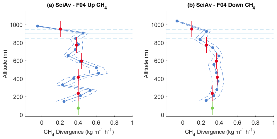
Figure 11 F04 CH₄ flux divergence profiles for the flight up (a) versus down (b). The profile shapes differ, with a much more variable flux divergence in the up profile.

4.3 AVIRIS-NG aircraft emissions estimates

Methods based on imaging spectroscopy (e.g., AVIRIS-NG, GHGSat) provide a unique opportunity for emissions estimation, validation of ground-based measurements, and to help develop satellite monitoring techniques, while also providing leak detection (Cusworth et al., 2019; Frankenberg et al., 2016; Tyner and Johnson, 2021). CH₄ emissions from the oil and gas industry are sporadic, with higher emissions only captured 20 %–35 % of the time when sampling (Duren et al., 2019). While the SciAv and TERRA methods have lower uncertainties than the AVIRIS-NG method, they require prior knowledge of presumed sources. Therefore, the mass-balance methods are unlikely to identify unknown sources located outside sampling boundaries. The persistence of large, sporadic emissions, along with their relation to sampling with or without operator notice, should be studied further. While AVIRIS-NG estimates are dependent on estimates of the wind speed and direction as well as repeated sampling to assess source trends, they avoid the mass-balance requirements of a stationary source and the need to extrapolate emissions to the surface (Duren et al., 2019). This is because AVIRIS-NG effectively samples the entire atmospheric column between the ground and the sensor as a “snapshot”.

In our study, the SciAv and TERRA algorithms yielded similar results when proper sampling conditions were met. While non-stationarity occurred for F04, the change in estimates between the upwards and downwards segments does not account for the large difference between the SciAv and AVIRIS-NG measurements of the Syncrude plant. Discrepancies between estimates due to missing, potentially large emissions below the lowest SciAv flight path are highly unlikely, as the F04 plume was “fully captured” with emissions decreasing towards the surface (Sect. S1.5). The substantially larger AVIRIS-NG estimate may be due to industrial operations, such a flaring or venting events. It is possible that only one of the two plumes observed by AVIRIS-NG were present when SciAv sampled, or that large day-to-day variability exists in CH₄ emissions. However, unlike the SciAv flight, operators were not informed before sampling, and operating conditions were not shared by the facility, so the underlying reason for this difference could not be evaluated. Due to the sporadic tendency of CH₄ emissions and the different sampling date, the AVIRIS-NG result is not directly comparable to the mass-balance algorithm's results for F04, but it can provide an idea of the range of potential emissions and specific source locations within the Syncrude plant. The SciAv and AVIRIS-NG methods have been independently compared and have been shown to provide consistently similar emissions estimates when employed under similar conditions (Frankenberg et al., 2016; Duren et al., 2019; Thorpe et al., 2020). Given the results of these studies, the AVIRIS-NG data captured on 14 August 2017 may not be anomalously high but could instead represent independent information on the variability of emissions from the region. Further work comparing these methods under similar conditions, along with greater transparency in facilities operations, could help confirm these conclusions and support more accurate emission budgets. The large emissions estimates from the same site outlines the importance of repeated sampling and the benefit of using multiple methods to characterize source behaviour, estimate the distribution of emissions from facilities, and estimate regional, national, and global emission budgets.

5 Conclusion

We found that emissions estimates were consistent between two top-down, mass-balance methods, providing confidence in these methods at a time when emissions reductions are needed. This finding is important, because airborne methods are used to validate top-down and bottom-up GHG emissions and to develop emissions inventories. When fundamental assumptions were met, the airborne mass-balance algorithms, SciAv and TERRA, produced similar estimates that agreed (3 %–25 %) within algorithm uncertainties (4 %–34 %). The two algorithms disagreed when the fundamental assumption of a stationary emission plume was not met (F04). Having increased confidence in estimates from the two mass-balance airborne methods provides a more certain foundation for policy and regulatory decisions. Including airborne imaging spectrometer emissions estimates in top-down regional budgets can provide additional information about emissions by capturing unknown sources or sporadic emissions. The ideal approach for characterizing and estimating GHG budgets would include repeated measurements, using a combination of airborne methods (in conjunction with new spectroscopic measurements from satellites for larger, continuous regional estimates), and by using ground-based equipment for small-scale point source quantification (Hardwick and Graven, 2016; National Academies of Sciences, Engineering, and Medicine, 2018; Saunois et al., 2020; Nisbet et al., 2020; Rutherford et al., 2021; Cusworth et al., 2022). Observations that combine and cross-validate multiple monitoring methods at varying scales of sampling will provide the most accurate modelling, improve GHG estimation, and help reconcile the often-reported gap between top-down and bottom-up estimates. Continued advances in developing more accurate inventories will allow for more effective policy and regulatory decisions that target the contribution of CO₂ and CH₄ to climate change.