Assessment of the error budget for stratospheric ozone profiles retrieved from OMPS limb scatter measurements

This study presents an error budget assessment for the ozone profiles retrieved at the University of Bremen through limb observations of the Ozone Mapper and Profiler Suite – Limb Profiler Suomi National Polar-orbiting Partnership (OMPS-LP SNPP) satellite instrument. The error characteristics are presented in a form that aims at being compliant with the recommendations and the standardizing effort of the Towards Unified Error Reporting (TUNER) project. Besides the retrieval noise, contributions from retrieval parameters are extensively discussed and quantified by using synthetic retrievals performed with the SCIATRAN radiative transfer model. For this investigation, a representative set of OMPS-LP measurements is selected to provide a reliable estimation of the uncertainties as a function of latitude and season. Errors originating from model approximations and spectroscopic data are also taken into account and found to be non-negligible. The choice of the ozone cross section is found to be relevant, as expected. Overall, we classify the estimated errors as random or systematic and investigate correlations between errors from different sources. After summing up the relevant error components, we present an estimate of the total random uncertainty on the retrieved ozone profiles, which is found to be in the 5 %–30 % range in the lower stratosphere, 3 %–5 % in the middle stratosphere, and 5 %–7 % at upper altitudes. The systematic uncertainty is mainly due to cloud contamination and model errors in the lower stratosphere and due to the retrieval bias at higher altitudes. The corresponding total bias exceeds 5 % only above 50 km and below 20 km. After computing the estimate of the overall random and systematic error components, we also provide an ex-post assessment of the uncertainties using self-collocated OMPS-LP observations and collocated Microwave Limb Sounder (MLS) data in a χ² fashion.

1 Introduction

The objective of this paper is to provide an extensive uncertainty estimate for ozone profiles retrieved at the University of Bremen from the Ozone Mapper and Profiler Suite – Limb Profiler (OMPS-LP) on board the Suomi National Polar-orbiting Partnership (SNPP) spacecraft, within the framework of the Towards Unified Error Reporting (TUNER) project, which aims at homogenizing the error reporting in the atmospheric remote sensing community (von Clarmann et al., 2020). An extensive error characterization of the retrieved ozone profiles is relevant for the correct usage of the ozone profiles, e.g., to avoid misinterpretation of retrieval results in atmospheric regions where the product is affected by a large uncertainty. Such estimation is also valuable for the validation of the product: in order to understand and assess the statistical significance of the differences between datasets, it is namely important to have an estimation of their random and systematic errors.

A study assessing the error budget for OMPS-LP ozone retrieval was conducted by NASA at the beginning of the satellite mission and reported by Rault and Loughman (2012). The authors described the retrieval algorithm, which has since been substantially changed (Kramarova et al., 2018), and presented the results of Monte Carlo simulations to estimate both bias and random components of the uncertainty on their profiles. The authors generated randomly perturbed forward simulations by accounting for the errors in a series of parameters, which were then fed into their standard retrieval routine. They estimated a bias within 4 % and a 4 % precision from 15 to 50 km, with aerosol, surface albedo, and height registration affecting the retrieval up to 10 %–15 % in the lower stratosphere (Rault and Loughman, 2012). A similar investigation of the error budget for the Scanning Imaging Absorption Spectrometer for Atmospheric Cartography (SCIAMACHY) ozone profiles V2.5 retrieved at the University of Bremen was presented by Rahpoe et al. (2013). The focus of that study was on parameter errors, and it reported an estimated random error of about 10 %–15 % and a systematic component of about 7 %. Recently, several satellite groups have been working on improving the uncertainty characterization of their own retrieval products within the TUNER initiative (e.g., Sheese et al., 2020).

Regarding the used terminology, we are aware of the effort of the Joint Committee for Guides in Metrology (JCGM) and the Bureau International des Poids et Mesures (BIPM) to replace the concept of error analysis with the concept of uncertainty analysis (Fox, 2010). Referring to von Clarmann et al. (2020), we define the term “error” as the difference between a reference (truth) and the value from measurements or simulations, whereas “uncertainty” describes the distribution of the error. However, in this work, as in von Clarmann et al. (2020), the two terms are not mutually exclusive, especially when used in combined terms, e.g., parameter error or error budget. We also define “ex ante” and “ex post” estimates according to von Clarmann et al. (2020). The terms “random” and “systematic” are used here to characterize error sources that mainly contribute to the variance and to the bias, respectively. This means that, when considering the average of several profiles, random contributions are expected to be reduced (proportionally to the square root of their number), whereas the systematic terms remain constant. Errors on level 1 (L1) data are not explicitly taken into consideration in this study but are rather assumed to be included in the signal-to-noise ratio (SNR) of the instrument, because it is currently not possible to attribute L1 errors to specific causes, and recent efforts from the NASA team largely mitigated the contributions from stray light and pointing (Kramarova et al., 2018; Glen Jaross, personal communication, 2020). Another source of error that is not considered in this study but is relevant for limb observations is related to the horizontal smoothing, tackled, for example, in von Clarmann et al. (2009); Cortesi et al. (2007). Namely, limb observations smooth the atmospheric variability over a 250–400 km region around the tangent point (TP) along the line of sight (Zawada et al., 2018). In addition, a 1-D retrieval cannot account for gradients along the line of sight, leading to an additional uncertainty component, which is not expected to be relevant on average but might play a role for atmospheric scenes characterized by strong gradients along the line of sight, e.g., in the presence of the ozone hole (Zawada et al., 2018) or sharp reflectivity gradients.

In this study, it was not possible to carry out an error budget for the entire dataset, for obvious computing time limitations. As a consequence, we focused on case studies accounting for variations in the geometry and observing conditions, whereas for the parameter and spectroscopic uncertainties, we provide a case sample that is considered to be representative of the entire dataset.

With this study, we intend to discuss and characterize in more detail the various error contributions, following the TUNER recommendations, and to complete the analysis with an ex post validation of the obtained error budget. This paper is structured as follows: after the presentation of the OMPS-LP instrument in Sect. 2.1 and of the retrieval algorithm with its characterization in Sect. 2.2, an assessment of the systematic retrieval error is described in Sect. 3. Parameter errors are extensively discussed in Sect. 4 as a function of altitude, latitude, and season. Uncertainties related to spectroscopic errors are discussed in Sect. 5, with a focus on the used ozone cross section, whereas uncertainties related to model approximations are presented in Sect. 6. Finally, an overall uncertainty estimate is reported in Sect. 7, followed by an ex post assessment of the reported errors using self-collocated OMPS-LP observations and a validation of the error budget using collocated MLS data in a χ² fashion.

2 Description of the instrument and of the retrieval scheme

2.1 OMPS-LP instrument

OMPS was launched by NASA at the end of 2011 on board the SUOMI-NPP satellite platform and started to collect data in January 2012 (Flynn et al., 2014). The spacecraft flies in a sun-synchronous orbit, with a nominal 13:30 local time ascending node. The main objective of the mission is the observation of the ozone vertical distribution within the Earth's middle atmosphere at high accuracy. The OMPS-LP instrument, of interest for this study, images the atmosphere by observing the Earth's limb backwards with respect to its flying direction (Jaross et al., 2014). It collects 180 images (i.e., atmospheric spectra) per orbit (around 160 with solar zenith angle less than 80^∘) and completes 14–15 orbits per day. The instrument measures limb scattered radiance in the spectral region between 280 and 1000 nm. It employs a prism spectrometer, resulting in a spectral resolution that degrades from 1 nm in the ultraviolet (UV) to 40 nm in the near infrared. It observes the altitude range from ground to ∼ 100 km, with an instantaneous field of view of about 1.5 km and a sampling of 1 km (Jaross et al., 2014).

2.2 Retrieval scheme

The official ozone product for OMPS-LP observations is released by NASA and described elsewhere – see, for example, Kramarova et al. (2018). This study assesses the error budget of the ozone profiles retrieved from OMPS-LP observations at the University of Bremen by using a nonlinear inversion technique with first order Tikhonov regularization. This study is based on the retrieval of ozone profiles from OMPS-LP observations developed at the University of Bremen, by implementing an iterative approach and the regularized inversion technique with first order Tikhonov constraints (Rodgers, 2000). The forward modeling accounts for the atmospheric multiple scattering in 1-D geometry within the framework of the approximate spherical solver of the SCIATRAN radiative transfer model (RTM) (Rozanov et al., 2014). The measurement vector y contains the logarithms of the normalized limb radiance at all selected tangent heights (TH) and spectral points; e.g., the elements referring to the TH j are defined as

$$\begin{array}{}\text{(1)}& {\mathit{y}}_j=\log \left({\displaystyle \frac{{\mathit{I}}_{{\mathrm{TH}}_j}}{{\mathit{I}}_{{\mathrm{TH}}_{\mathrm{norm}}}}}\right)-{\mathit{P}}_n,\end{array}$$

where a normalization to a limb measurement at an upper TH is performed. For a detailed description of the retrieval algorithm, we refer to Arosio et al. (2018). In this study, we used very similar settings to choose spectral segments and the altitude ranges; Table 1 lists the details of the used wavelengths and normalization altitudes. The order of the subtracted polynomial (P_n in Eq. 1) in each spectral segment is also reported in the last column of Table 1. The a priori profile is set to zero: this means that, at each iteration, SCIATRAN constrains the difference between zero and the ozone profile itself.

Table 1 List of the spectral segments considered in the ozone retrieval, with corresponding TH range, altitude used for the normalization, and order of the subtracted polynomial ( “–” means that no polynomial is subtracted).

Ozone, NO₂, and O₄ have relevant spectral signatures in the selected spectral ranges. Their respective cross-sections are taken from Serdyuchenko et al. (2014a) and Bogumil et al. (2000) and are pre-convolved to the OMPS-LP spectral resolution. Ancillary information regarding background temperature and pressure for each OMPS-LP observation is provided in L1 data and comes from the Goddard Earth Observing System (GEOS)-5 model.

The OMPS-LP SNR is estimated from the residuals between the measured and the modeled spectrum. This is done at a pre-processing step, where, in addition, a “shift and squeeze” spectral correction is applied in the Chappuis band, located in the visible spectral range. This correction is applied independently for each TH between 10 and 31 km and consists, as the name implies, in the calculation of a shift and a squeeze parameter, which defines the wavelength correction Δλ for each wavelength grid point of the modeled spectrum relative to the measured one. This correction is meant to account for potential issues with the spectral calibration and a possible thermal expansion of the sensor. Due to the relatively low spectral resolution of OMPS-LP, the fine-scale absorption structure in the UV is mostly not resolved. As a consequence, the UV retrieval uses normalized radiances or their slopes rather than the differential structure, and the influence of spectral misalignments is expected to be negligible so that the shift and squeeze algorithm is not applied.

Simultaneously with the ozone retrieval, the surface albedo estimation is performed by exploiting the sun-normalized radiance: the two spectral intervals 355–365 and 670–680 nm are used where the ozone absorption has a minimum. Beforehand, a cloud filter is also applied, and the retrieval of aerosol extinction profiles is performed (see Arosio et al., 2018 for more details).

2.3 Retrieval characterization and retrieval noise

To characterize the retrieval algorithm, the averaging kernels (AKs) and the retrieval noise covariance matrix S_x,noise are analyzed. AKs provide the information content of the measurements and the sensitivity of the retrieval as a function of altitude. Following (Rodgers, 2000), they are defined for our case as follows:

$$\begin{array}{}\text{(2)}& {\displaystyle }\begin{array}{rl}{\mathbf{S}}_{x,\mathrm{noise}}=& {\left({\mathbf{K}}^T{\mathbf{S}}_{y,\mathrm{noise}}^{-\mathrm{1}}\mathbf{K}+{\mathbf{S}}_{x,\mathrm{reg}}\right)}^{-\mathrm{1}}{\mathbf{K}}^T{\mathbf{S}}_{y,\mathrm{noise}}^{-\mathrm{1}}\mathbf{K}\\ & {\left({\mathbf{K}}^T{\mathbf{S}}_{y,\mathrm{noise}}^{-\mathrm{1}}\mathbf{K}+{\mathbf{S}}_{x,\mathrm{reg}}\right)}^{-\mathrm{1}},\end{array}\text{(3)}& {\displaystyle }\mathbf{A}={\left({\mathbf{K}}^T{\mathbf{S}}_{y,\mathrm{noise}}^{-\mathrm{1}}\mathbf{K}+{\mathbf{S}}_{x,\mathrm{reg}}\right)}^{-\mathrm{1}}{\mathbf{K}}^T{\mathbf{S}}_{y,\mathrm{noise}}^{-\mathrm{1}}\mathbf{K},\end{array}$$

where K is the weighting function matrix, S_y,noise is the measurement noise covariance matrix, and S_x,reg is the used regularization matrix. Typical values of the retrieval noise σ_{x,ret noise}, i.e., the square root of the diagonal elements of S_x,noise, averaged over one month, are reported, expressed as a percentage of the true profile, as a function of altitude and latitude in Fig. 1.

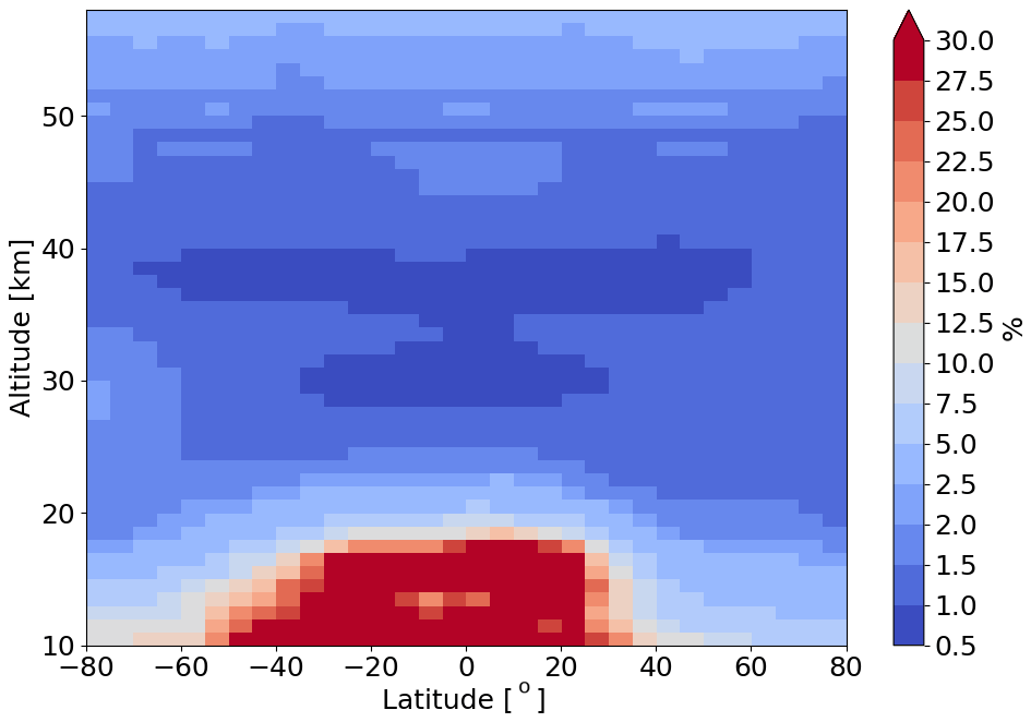
Figure 1 Monthly and zonally averaged retrieval noise for March 2016 as a function of altitude and latitude.

The retrieval noise associated with the ozone profiles does not show any significant latitudinal dependence above 25 km. It lies in the range of 1 %–4 % up to 60 km and tends to increase up to 10 %–30 % at lower altitudes, particularly in the tropical upper troposphere–lower stratosphere (UTLS), where the ozone concentration drops significantly and the retrieval sensitivity degrades.

Figure 2 Vertical resolution (a) and measurement response (b) for the standard retrieval version over 1 d (15 March 2016).

The vertical resolution of the retrieved profiles is computed as the inverse of the diagonal elements of the AK, multiplied by the altitude layer width, whereas the measurement response is defined as the area of the AK and gives an estimate of the a priori contribution (Rodgers, 2000), and it is dimensionless. The vertical resolution and the measurement response are reported in Fig. 2, averaged over 1 d. Below 30 km, the vertical resolution of the retrieval scheme is typically about 2.5–3 km and is worst around 33 km, where the transition of the sensitivity between UV and Chappuis spectral ranges occurs. The best vertical resolution of the profiles is achieved around 45 km, whereas above 50 km, it gets coarser due to the increasing regularization. The measurement response is shown in Fig. 2b and stays around 1.0 at most of the altitudes, except below 15 km in the tropics.

3 Synthetic retrievals using the Monte Carlo approach

Firstly, by using synthetic retrievals with the Monte Carlo approach, we evaluate the systematic component of the retrieval error and assess the linearity of the error propagation within the retrieval scheme.

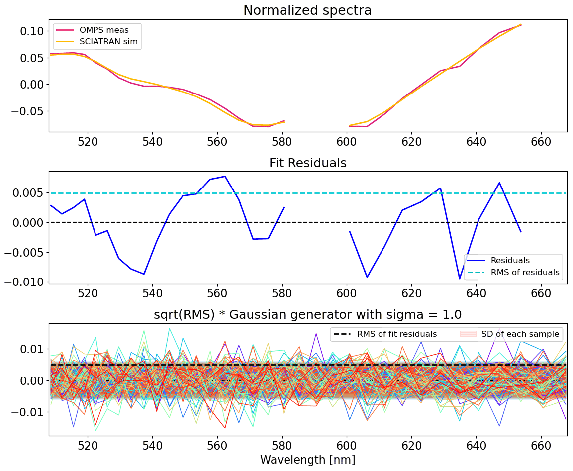
Figure 3 Example of spectra, fit residuals, and randomly generated noise sequences (multiplied by $\sqrt{\mathrm{RMS}}$) in the Chappuis band. The square root of the fit residuals (rms) is equal to the standard deviation (SD) of each generated noise sample.

The following procedure is implemented. The SCIATRAN v4.0 forward model is run in OMPS-LP observation geometry, obtaining a synthetic OMPS-LP spectrum. This is then fed into the standard retrieval described in Sect. 2.2. Since, in the retrieval scheme, the SNR of the measurements is estimated from the residual fit, a similar procedure is implemented for the synthetic cases. First, the root mean square (rms) of the fit residuals at every altitude and for each spectral segment is computed using OMPS-LP data for a standard retrieval run of the same state. This rms is used as the estimated SNR of the measurement. Then, a Gaussian generator is implemented to randomly generate N=50 noise sequences. Figure 3 shows, in the upper panel, an example of residual fits, i.e., the difference between OMPS-LP and the fitted model spectrum, together with the 50 generated noise samples, in the Chappuis band. The noise sequences are then multiplied by the SNR value estimated from the real measurements and added to the synthetic spectrum previously simulated. In this way, we obtained 50 intensity matrices, which are fed into the retrieval scheme to get unperturbed ozone profiles, ${\mathit{O}}_{\mathrm{3}}^{n,\mathrm{unpert}}$. We use the ozone profile retrieved from the real measurements as first guess profiles, and we refer to it as the ”true” ozone, which is then compared with the average of the retrieved unperturbed ozone profiles. Figure 4a shows all 50 retrieved unperturbed profiles (with different noise sequences applied) and their average ${\mathit{O}}_{\mathrm{3}}^{\mathrm{avg},\mathrm{unpert}}$, in black, for one selected OMPS-LP state. Rigorous definitions of the average retrieved unperturbed ozone profile and the difference to the true profile δ_x,unpert, as function of latitude (ϕ) and altitude (z), are given below:

$$\begin{array}{}\text{(4)}& {\displaystyle }{\mathrm{O}}_{\mathrm{3}}^{\mathrm{avg},\mathrm{unpert}}(\mathit{\varphi },z)={\displaystyle \frac{\mathrm{1}}{N}}\sum _{n=\mathrm{1}}^N{\mathrm{O}}_{\mathrm{3}}^{n,\mathrm{unpert}}(\mathit{\varphi },z),\text{(5)}& {\displaystyle }{\mathit{\delta }}_{x,\mathrm{unpert}}(\mathit{\varphi },z)={\displaystyle \frac{{\mathrm{O}}_{\mathrm{3}}^{\mathrm{true}}(\mathit{\varphi },z)-{\mathrm{O}}_{\mathrm{3}}^{\mathrm{avg},\mathrm{unpert}}(\mathit{\varphi },z)}{{\mathrm{O}}_{\mathrm{3}}^{\mathrm{true}}(\mathit{\varphi },z)}}\times \mathrm{100}.\end{array}$$

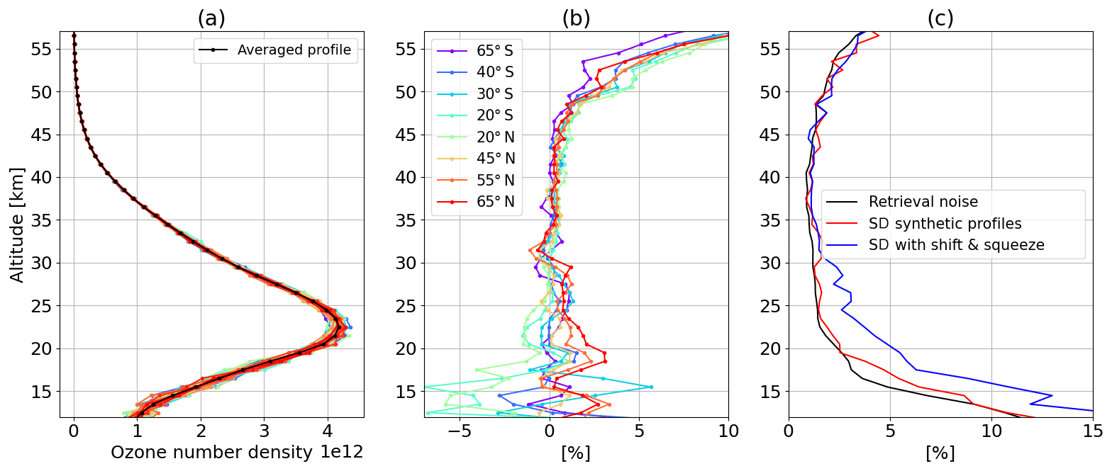
Figure 4 (a) All 50 retrieved unperturbed ozone profiles with their average in black. (b) Relative differences δ_x,unpert at several latitudes. (c) Retrieval noise and standard deviation of the synthetic retrievals with and without shift and squeeze procedure.

Figure 4b displays the average relative difference δ_x,unpert for several latitudes. The relative discrepancy is significantly different from zero, contrary to what is ideally expected, particularly above 50 km, where the discrepancy increases with altitude up to 5 %–10 %. In addition, in the lower stratosphere, significant differences are observed, with peaks of 2.5 %–5 % below 20 km; however, their sign changes with the latitude and has an oscillating nature. These discrepancies are related to the fact that we choose as a priori the null profile and that SCIATRAN regularizes, at each iteration, the difference between zero and the resulting ozone profile. As a consequence, at altitudes where the Tikhonov regularization becomes stronger, the retrieved ozone profile tends to be underestimated. The large relative differences are also related to the very low ozone values at the upper altitudes. This feature is a component of the systematic error of the retrieved profiles and has to be taken into account when comparing the dataset with other reference instruments. In Fig. 4c, the retrieval noise and the standard deviation of the unperturbed synthetic retrievals are plotted together in relative values for a direct comparison. As soon as the shift and squeeze procedure is activated, the standard deviation of the synthetic profiles increases drastically. The maximum range of the shift and squeeze correction allowed in the retrieval is ±1 nm, resulting in an increase of the noise error by about 50 % compared to the linearly propagated retrieval noise. This implies that the error propagation below 30 km has a non-linear component related to the shift and squeeze algorithm. This term has to be taken into account in the total error estimation and will be identified as σ_{x,shift&squeeze}. Otherwise the measurement noise is fairly linearly propagated into level 2 (L2) profiles.

By using synthetic simulations, we also checked the dependence of the retrieved ozone profile on the first guess profile, and it was found to be negligible (not shown here). When the first guess profile was scaled by values between −50 % and +100 %, the retrieval scheme showed strong stability, with the resulting ozone profile being affected by less than 1 %, as expected by Fig. 4b.

4 Parameter uncertainty

In this section, we discuss the so-called parameter errors, i.e., the uncertainty components originating from using certain information about the atmospheric state, which is either known or independently retrieved with a certain error and which does not enter the state vector. The following parameters are considered: surface albedo, aerosol extinction profile, TH registration, pressure, and temperature profiles. For each parameter, a reasonable value of its error is estimated, corresponding to their standard deviation, and used to generate perturbed scenarios and synthetic retrievals. Table 2 indicates the five considered parameters and the values of their respective estimated errors.

Table 2 List of the parameters used for the sensitivity studies and respective values of the variations, i.e., their standard deviation, corresponding to their estimated errors.

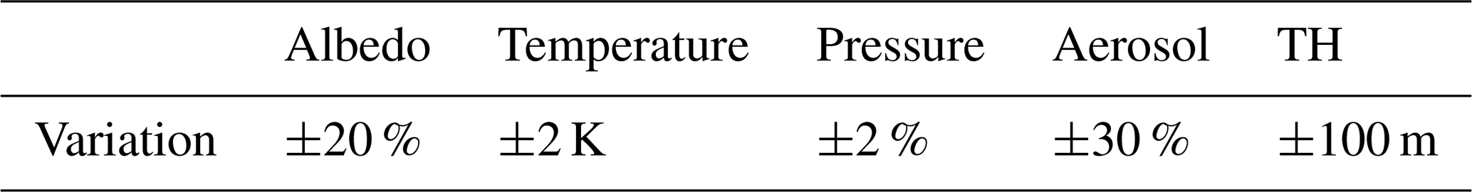
The magnitudes of these errors are either estimated from the retrieval product, e.g., for aerosol extinction profiles, or are taken from literature. Temperature and pressure profiles are taken from the GEOS-5 global assimilation model, and a reasonable estimation of their precision is 2 K and 2 %, respectively – see, for example, Langland et al. (2008). These estimates were also reported, for example, by Nowlan et al. (2007), who studied the differences between MAESTRO and reanalysis from the National Centers for Environmental Prediction (NCEP) and the European Centre for Medium-range Weather Forecasts (ECMWF). The aerosol extinction retrieved at the University of Bremen (for reference Malinina et al., 2018) shows, on average, an upper error value of about 30 % in the lower stratosphere. Similarly, an estimate of 20 % precision as an upper boundary value for the surface albedo comes form the analysis of the results of the surface albedo retrieval, performed at the same time as ozone. Finally, an important parameter for ozone limb retrievals is the pointing knowledge of the instrument. According to Moy et al. (2017), the results from NASA investigations about the pointing stability of the instrument indicate that OMPS-LP pointing has an accuracy of about ±100 m. The final uncertainties on ozone profiles related to the errors in albedo, temperature, pressure, aerosol extinction, and tangent height registration are indicated in following as σ_x,albedo, σ_x,T, σ_x,P, σ_{x,aerosol ext}, and σ_x,TH, respectively.

To have a representative sample of cases for the parameter uncertainty estimation, we selected cloud-clear OMPS-LP cases distributed over one year of observations, with the aim to have about 50–100 cases distributed in 4 seasons and 5 latitude bands (southern and northern polar latitudes, southern and northern mid-latitudes, and the tropics). All estimated errors are assumed to have a random nature, as we have no information about systematic deviations of the parameters. It has to be noted that for aerosol, temperature, and pressure, the error on parameter was assumed to be constant in altitude, even though a random perturbation as a function of height might also be assumed. A comparison of the resulting error can be found in the Supplement.

4.1 Methodology

The Monte Carlo approach described in Sect. 3 has been also used to study the parameter uncertainty of the retrieval. In this case, one parameter at a time is varied in the forward model, then the Gaussian noise is added to the simulated radiances in the same way as described above; N intensity matrices are obtained, which are fed into the retrieval scheme to get perturbed ozone profiles, ${\mathit{O}}_{\mathrm{3}}^{n,\mathrm{pert}\mathrm{\_}\mathrm{fix}}$. We then define the averaged perturbed ozone profiles ${\mathit{O}}_{\mathrm{3}}^{\mathrm{avg},\mathrm{pert}\mathrm{\_}\mathrm{fix}}$ and the relative differences with respect to the averaged unperturbed retrievals (${\mathit{O}}_{\mathrm{3}}^{\mathrm{avg},\mathrm{unpert}}$) as follows:

$$\begin{array}{}\text{(6)}& {\displaystyle }{\mathrm{O}}_{\mathrm{3}}^{\mathrm{avg},\mathrm{pert}\mathrm{\_}\mathrm{fix}}(\mathrm{param},\mathit{\varphi },z)={\displaystyle \frac{\mathrm{1}}{N}}\sum _{n=\mathrm{1}}^N{\mathrm{O}}_{\mathrm{3}}^{n,\mathrm{pert}\mathrm{\_}\mathrm{fix}}(\mathrm{param},\mathit{\varphi },z),\text{(7)}& {\displaystyle }\begin{array}{rl}& {\mathit{\sigma }}_{x,\mathrm{pert}\mathrm{\_}\mathrm{fix}}(\mathrm{param},\mathit{\varphi },z)=\\ & {\displaystyle \frac{{\mathrm{O}}_{\mathrm{3}}^{\mathrm{avg},\mathrm{pert}\mathrm{\_}\mathrm{fix}}(\mathrm{param},\mathit{\varphi },z)-{\mathrm{O}}_{\mathrm{3}}^{\mathrm{avg},\mathrm{unpert}}(\mathit{\varphi },z)}{{\mathrm{O}}_{\mathrm{3}}^{\mathrm{avg},\mathrm{pert}\mathrm{\_}\mathrm{fix}}(\mathrm{param},\mathit{\varphi },z)+{\mathrm{O}}_{\mathrm{3}}^{\mathrm{avg},\mathrm{unpert}}(\mathit{\varphi },z)}}\times \mathrm{200},\end{array}\end{array}$$

where n is the running number of the noise sequence; σ_{x,pert_fix} provides an estimate of the effect of each parameter error on the retrieved ozone profile. In this case, we assume a fixed error value on the parameters and evaluate its effect in the ozone space.

Another conceptually similar approach consists in perturbing a single parameter around its mean value by a normally distributed amount, which has a standard deviation equal to the estimated parameter error. For example, the aerosol extinction profile is perturbed by 30 % so that 50 aerosol extinction profiles normally distributed around the original one are created. The standard retrieval version is then applied 50 times to the synthetic OMPS-LP spectra with perturbed parameters, using the residual fit from the corresponding retrieval of measured data as SNR. The quantity of interest, i.e., the random uncertainty on the retrieved ozone, is the standard deviation of the retrieved ozone profile distribution.

$$\begin{array}{}\text{(8)}& \begin{array}{rl}& {\mathit{\sigma }}_{x,\mathrm{pert}\mathrm{\_}\mathrm{rand}}(\mathrm{param},\mathit{\varphi },z)=\\ & {\displaystyle \frac{\mathrm{SD}\left({\mathrm{O}}_{\mathrm{3}}^{n,\mathrm{pert}\mathrm{\_}\mathrm{rand}}(\mathrm{param},\mathit{\varphi },z)\right)}{{\mathrm{O}}_{\mathrm{3}}^{\mathrm{avg},\mathrm{unpert}}(\mathit{\varphi },z)}}\times \mathrm{100}\end{array}\end{array}$$

4.2 Results

Synthetic simulations using the two methods described above are performed to assess the impact of errors of the forward model parameters on the retrieved ozone profiles. In this investigation, the shift and squeeze in the Chappuis band was turned on, as in the standard retrieval version, with the upper limit for the Δλ equal to 1 nm. As defined by Eqs. (7) and (8), for the rest of the analysis, the differences are computed relative to ${\mathit{O}}_{\mathrm{3}}^{\mathrm{avg},\mathrm{unpert}}$ rather than to the true ozone profile in order to have an evaluation of the sensitivity of the retrieved ozone profile to forward model parameters, which is not affected by the sensitivity of the retrieval itself. Below 20 km, it is challenging to estimate the effect of each particular parameter because of a high variability found in the simulations, which is, however, reduced by averaging over several case studies.

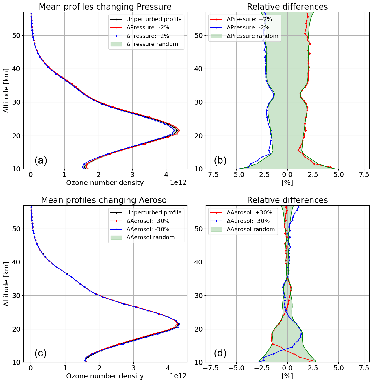
Figure 5 In panels (a) and (c), the unperturbed ozone profile is shown together with the mean ozone profiles obtained by a Monte Carlo approach by perturbing the forward simulation pressure (a, b) and aerosol extinction (c, d) by 2 % and 30 %, respectively. The green shaded area shows (barely visible) the standard deviation of the 50 profiles obtained with the second approach. In panels (b) and (d), σ_{x,pert_fix} and σ_{x,pert_rand} are shown in relative values for the respective cases.

In Fig. 5, an example of the comparison between the results of the two methodologies described above is presented for a single OMPS-LP observation for pressure and aerosol extinction cases. The plot indicates that both approaches lead to very similar results. In both cases, the perturbed profiles are shown in the left panels in red and blue. The unperturbed one is shown in black, whereas the green shaded area represents the standard deviation of the N simulations from the second approach (σ_{x,pert_rand}). For a better view, in the right panels, σ_{x,pert_fix} and σ_{x,pert_rand} are plotted.

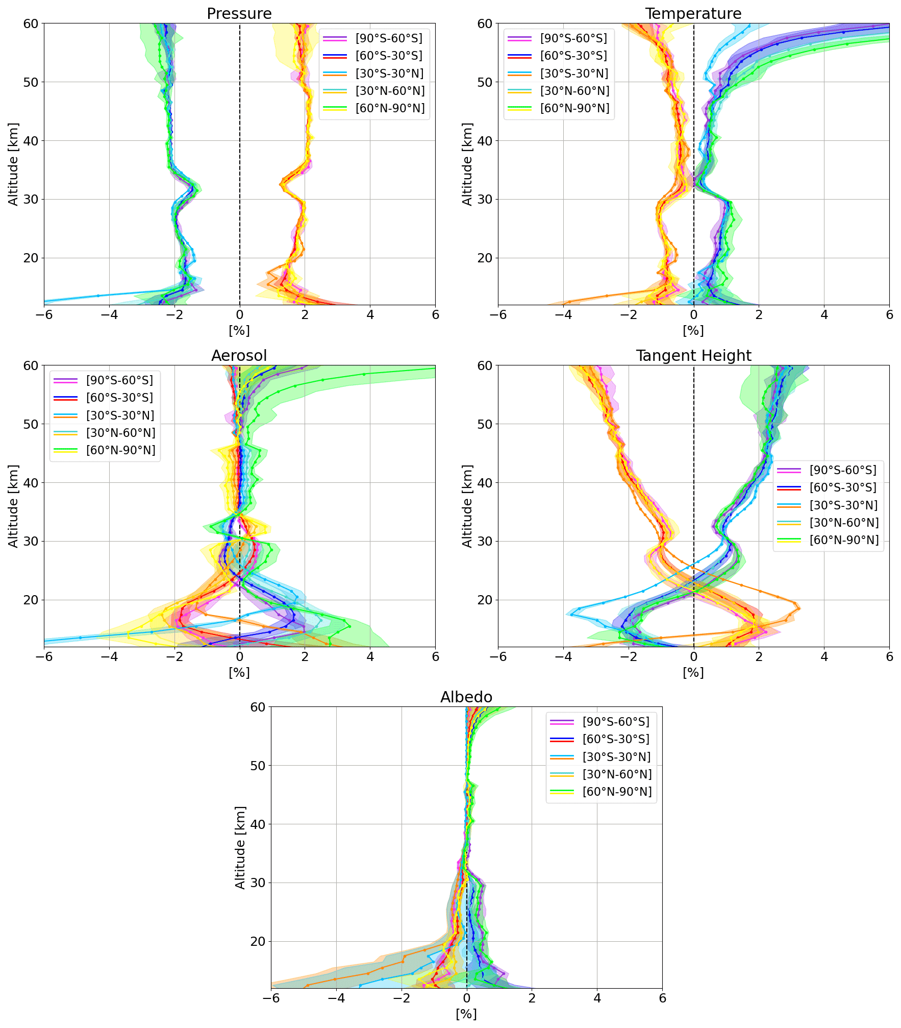
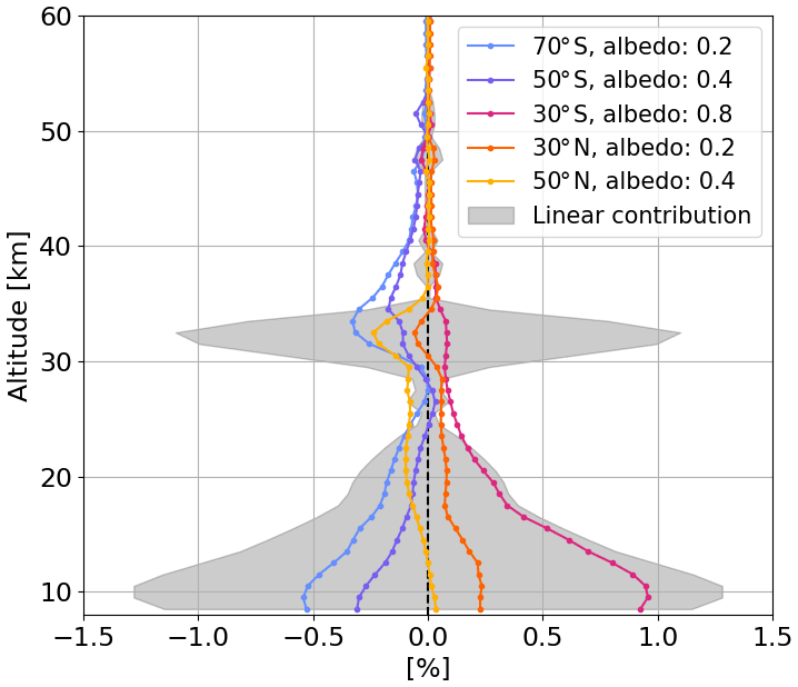
Figure 6 Estimation of parameter errors from synthetic retrievals in terms of the relative uncertainty on the ozone profile. Each panel refers to the parameter specified in the title, which is perturbed according to Table 2. Warm colors indicate a positive perturbation of the parameter, cold colors a negative one. Latitude bands are indicated in the legend, and the shaded areas around each profile indicate the scattering of the uncertainty as a function of season.

After verifying the agreement between the two methods, the final results will be reported using the first approach (fixed parameter perturbation), which is computationally less demanding and conveys information on the relationship between the sign of the parameter perturbation and the sign of the consequent ozone perturbation. In Fig. 6, the results of the parameter uncertainties are reported for the 5 identified parameters as a function of latitude (as reported in the legends) and for both increment and decrement of the parameter. To give an indication of the variability in term of season, the shaded areas indicate the standard deviation of the uncertainties in different seasons.

From the upper left panel of Fig. 6, we notice that the effect of perturbing the pressure profile is fairly constant with height, with a deviation of 2 %–3 % relative to the unperturbed case at most of the altitudes, without a significant dependence on latitude or season, though a larger scatter is seen at high latitudes. A reduction of the sensitivity of the retrieval at about 32–33 km is the reason for the reduced effect of the perturbation, and it is also visible in other panels.

The effect of increasing the temperature profile by Δ=2 K has a different sign and a smaller amplitude with respect to the pressure perturbation, leading to an underestimation of the retrieved ozone, with the largest effects below 30 km and in the upper stratosphere. However, the deviations remain within 1 %–2 % at all altitudes above 15 km, and no evident variation as a function of latitude is detected, except above 50 km, where an underestimation of the temperature leads to a large overestimation of ozone.

The aerosol perturbation also has an inverse dependency on the ozone deviation, and the largest effect is observed below 25 km. A positive variation of the aerosol extinction leads to an underestimation of the ozone concentration, and it has the maximum impact at northern high latitudes due to the scattering geometry of the satellite observations: in the northern hemisphere, the forward scattering makes the effect of the aerosols stronger than the backward scattering observed in the southern hemisphere due to the stronger forward peak in the aerosol phase function. The dispersion of the values as a function of season is also large in the northern polar regions.

As already mentioned, for limb retrievals, the accurate knowledge of the instrument pointing is a highly relevant parameter. A perturbation of the TH of ±100 m leads to an uncertainty profile that changes sign at 20–25 km, with values increasing with altitude up to 3 %–4 % above 55 km.

In order to assess the impact of the retrieved surface albedo error on the ozone profile, we perturb the surface albedo value in the forward simulation and retrieve ozone, switching off the albedo retrieval. We find that the deviation from the unperturbed case is evident only below 30 km and appears to be symmetric in response to a positive or negative perturbation of the surface albedo: an increase of this parameter in the forward model leads to an underestimation of the ozone retrieved profile in the lower stratosphere and vice versa. The average unperturbed surface albedo values are reported in the legend for the displayed latitude bands.

We investigated whether parameter errors have an additive (i.e., their absolute values are independent from ozone concentration) or multiplicative (i.e., they scale with the ozone profile and have a constant relative values) nature. This is done by performing the simulations with a first-guess ozone profile scaled by ±20 % and comparing the results with Fig. 6. It was found that all parameter uncertainties are multiplicative: by doubling the amount of ozone, the relative error stays constant. Only for the aerosol extinction case we notice a stronger than linear dependence on the ozone amount, i.e., the relative error in ozone due the assumed background aerosol profile increases slightly with increasing ozone. In addition, since the errors on the parameters are random, we assume that the resulting ozone uncertainties are generally random as well. However, possible systematic effects along the time series cannot be excluded, particularly for what concerns the aerosol extinction contribution, which depends on the aerosol loading. As shown, the magnitude of the aerosol error also has a systematic variation along the latitude.

4.3 Clouds

Synthetic simulations have been performed to assess the effect of undetected clouds on the ozone profile; forward simulations are performed by adding a cloud layer in SCIATRAN using three scenarios: a cloud layer at 16–18, 10–12, and 4–6 km. Three optical depth (OD) values for each cloud altitude are also chosen: 0.1, 0.5, and 1.0. These are relatively small values to simulate thin clouds that could remain undetected by the implemented cloud filter. However, by applying the cloud filtering to the simulated intensities, the cases with OD of 0.5 and 1.0 are always flagged as cloudy by our algorithm. Clouds are assumed to consist of hexagonal ice crystals for the first two high-clouds and of water droplets for the lower-cloud case. The scenarios with an ice cloud of OD of 0.5 or 1.0 at 17 km refer to a typical thin cirrus in the tropics; the other two refer to a thin ice or low water cloud at mid- or high- latitudes. The cloud is added in the forward simulation, and the retrieval is performed with the standard settings using the SNR from an OMPS-LP retrieval. At the same time, a reference synthetic retrieval is run, i.e., a forward simulation without cloud, followed by a standard retrieval in the same way as for cloud-perturbed cases. For each altitude, the difference is then computed with respect to this reference unperturbed scenario:

$$\begin{array}{}\text{(9)}& {\mathit{\delta }}_{x,\mathrm{cloud}}={\mathrm{O}}_{\mathrm{3}}^{\mathrm{unpert}}-{\mathrm{O}}_{\mathrm{3}}^{\mathrm{pert}}.\end{array}$$

Figure 7 displays these relative differences for several ODs and cloud heights (for each panel). The shaded areas show the spread of the relative differences as a function of latitude within one orbit.

Figure 7 Relative difference between unperturbed and perturbed retrieved ozone profiles, with three different cloud scenarios ((a) water cloud at 7 km, (b) ice cloud at 10 km, (c) ice cloud at 18 km) represented by the gray horizontal bars for three optical depths (in different colors). The shaded areas give an idea of the spread of the differences as a function of latitude.

The discrepancies are generally positive, meaning that the presence of an undetected cloud leads to an underestimation of the ozone concentration, and increase, as expected, as a function of optical depth. Above 20 km, the differences are generally negligible, and the largest values are found in the case of a low-level water cloud, with deviations up to 15 %–20 % below 15 km in the tropics. An undetected thin cirrus affects the retrieved ozone with a deviation of 1 %–3 % between 20 and 30 km. The nature of these uncertainties is rather systematic, as thin clouds may not be filtered out by the employed cloud flag. As a consequence, the term δ_x,clouds will be added in the “systematic bias” δ_x,sys in Sect. 7.

5 Ozone cross section uncertainty

The uncertainty related to the ozone absorption cross section used in the retrieval has a relevant contribution to the error budget. A general problem for these considerations is the lack of precise information about the errors as a function of wavelength of the used cross sections (von Clarmann et al., 2020). In our case, we decided first to have a look at the impact on the retrieved profile of changing the cross section source and then to propagate an estimation of the cross section error into the ozone profile.

5.1 Changing cross section

We consider the following four cross sections: Serdyuchenko (SER, Serdyuchenko et al., 2011; Gorshelev et al., 2014), Bass and Paur (BP, Bass and Paur, 1985), Brion-Daumont-Malicet (BDM, Daumont et al., 1992; Malicet et al., 1995), and Voigt (Voigt et al., 2001). It should be borne in mind that different cross sections are reported at different resolutions, spectral ranges, and temperatures. BP and BDM are considered for our case only in the UV band, as they do not cover the entire wavelength range needed in the visible spectral range for all temperatures. In contrast, the Voigt cross section covers the entire Chappuis band but is available for fewer temperatures than SER. All cross sections have been convolved to OMPS-LP resolution before use. Figure 8 reports the relative differences for the ozone profiles retrieved, with the listed cross sections with respect to the standard SER case, averaged over one orbit. The shaded areas display the range of variations observed as a function of latitude or field of view within one orbit.

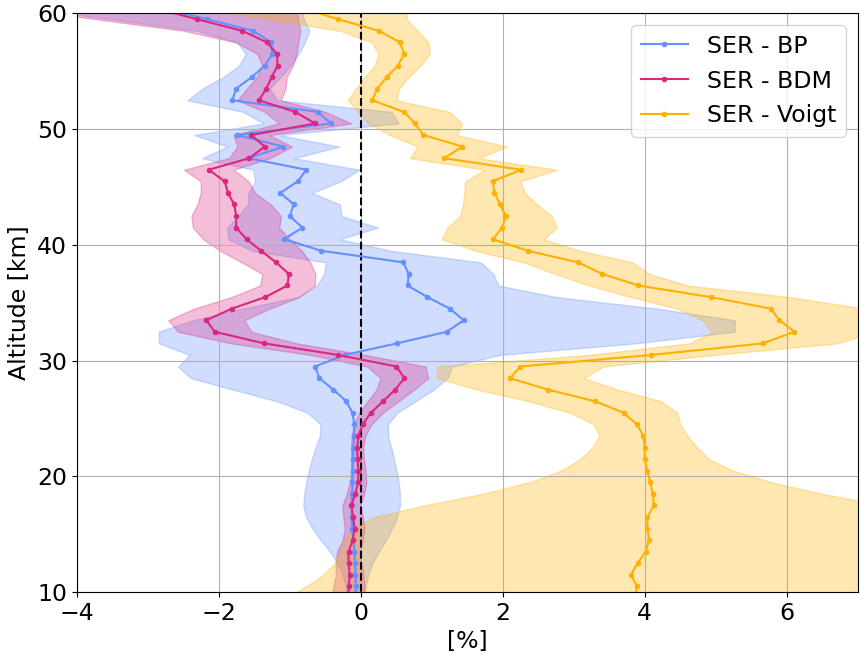
Figure 8 Relative differences between the ozone profiles retrieved considering different cross sections, with SER case used as a reference.

The obtained uncertainty is up to 6 % when considering the Voigt cross section and within ±2 % when comparing with the BP and BDM cases. The last two are of particular interest, as they are used (or were used) in the UV retrievals from NASA and University of Saskatchewan for OMPS-LP (Kramarova et al., 2018; Zawada et al., 2018).

5.2 Uncertainty propagation

The SER ozone cross section was measured for 11 temperature values in a broad spectral range covering from 213 to 1100 nm by using Fourier transform and Echelle grating spectrometers. According to Weber et al. (2016), in the UV spectral region, the wavelength-dependent total error on the cross section is in the range of 1 %–3 %. In this region, the light source stability and the detector noise play a dominant role, and as a consequence, the error has a noise-like, random nature. In the Chappuis band, on the contrary, the light source stability improves, whereas the optical densities used for the measurements are lower, leading to an overall error of about 2 %, with a predominant bias-like nature.

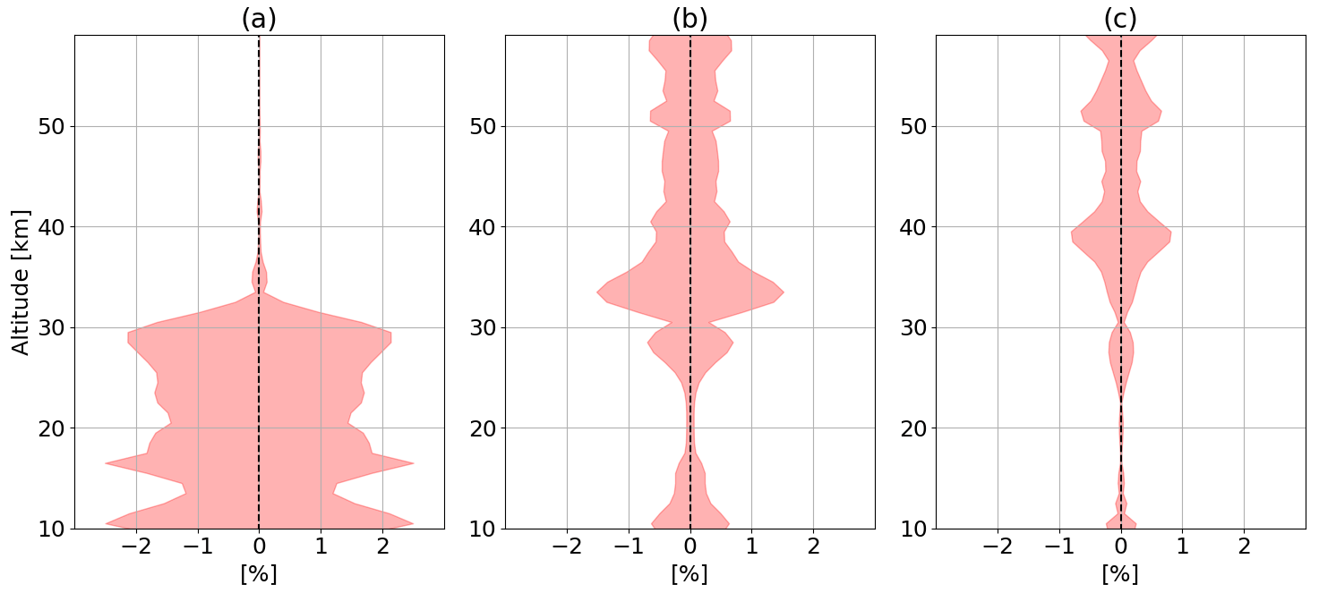
Figure 9 Standard deviation of 50 retrieved ozone profiles using a perturbed cross section: in panel (a) adding a random bias of 2 % (constant over wavelength) in the Chappuis band, and in panel (b) adding random noise with an amplitude of 2 % in the UV. (c) Standard deviation of 50 ozone profiles after perturbing the temperature and pressure profiles to investigate the uncertainty from the cross section temperature dependence.

As a consequence, the SER cross section is first perturbed by adding a normally distributed random bias with an amplitude of 2 % in the Chappuis band, obtaining 50 perturbed cross sections used to retrieve a corresponding number of ozone profiles. Figure 9 shows the standard deviation of the retrieved profiles, which gives an estimation of the uncertainty on ozone due to the error on the cross section. Uncertainties for the UV are computed in a similar way: N=50 randomly generated error sequences, with an amplitude equal to 2 % of the cross section value, are added to the SER cross section and used for the ozone retrieval. The standard deviation of the 50 retrieved ozone profiles is shown in the middle panel of Fig. 9. For both cases, the reported values refer to an average of the results over several synthetic simulations at different latitudes. The cross section uncertainty in the visible spectral range leads to a larger contribution with respect to the uncertainty in the UV, anyway within 2 %.

The term δ_x,cs is considered to be systematic, as the actual unknown noise sequence affecting the used cross sections is the same for all retrievals. The uncertainty on ozone is then expected to be of the magnitude estimated via the synthetic retrievals and constant for all observations, though with unknown sign. We also checked how the cross section error scales with the ozone amount and found that this error component is also multiplicative: by doubling the amount of ozone, the relative error is found to be fairly constant. We finally performed the synthetic simulations for the same case samples used for the parameter uncertainties in order to better check the variation of this component as a function of latitude and season without finding any relevant dependence, except for a general increase of the values at high solar zenith angles.

Errors from the temperature dependency of the ozone cross section have also been taken into consideration, similarly to Rahpoe et al. (2013): the temperature profile is perturbed by 2 K, and the pressure is accordingly changed to keep the air density equal to the unperturbed case. A total of 50 perturbed scenarios are generated, and the standard retrieval is run. The standard deviation of the synthetic retrievals is shown in Fig. 9c, averaged over one orbit, and this term is within ±0.5 %, with largest value at about 40 km.

6 Model errors

Model errors refer to the approximations in the RTM used for the ozone retrieval. In order to keep the processing time reasonable, it is required to use a number of simplifications in the model simulations, with the goal of both guaranteeing computational efficiency and keeping the error at the same level as the measurement uncertainties (von Clarmann et al., 2020). In this study, we focus our analysis on the scattering approximations and the radiative solver used in SCIATRAN by considering the geometries typically covered over an OMPS-LP orbit.

Figure 10 (a) Relative difference in the ozone profiles for different RT solvers and approximations for atmospheric sphericity. (b) Relative differences when changing scattering approximation and computation accuracy.

First, the radiative transfer solver in SCIATRAN can be chosen between the scalar discrete ordinate method (DOMS) and the combined differential-integral (CDI) approach (Rozanov et al., 2001). The difference in the ozone profiles retrieved using different solvers while keeping all other settings constant is shown in Fig. 10a, averaged over one orbit, and it is within 3 % at all altitudes. In addition, the approximation used in the RTM regarding the Earth's sphericity also plays a non-negligible role. In the standard retrieval version, the CDI solver uses the so-called approximate spherical solution, which estimates the multiple scattering contribution by integrating the pseudo-spherical radiative field along a line of sight crossing a “spherical atmosphere” (Rozanov et al., 2001). To test its accuracy, a comparison is performed with a model run including an additional iteration over the multiple scattering field, leading to a fully spherical solution. The difference shown in Fig. 10a is 0.5 %–1 % below 35  km and negligible above. The third curve in Fig. 10a refers to the “convolution case”, i.e., the difference between the standard profile retrieved from a synthetic spectrum and a profile retrieved from a synthetic spectrum that is simulated at high resolution, multiplied by a high-resolution solar spectrum, convolved at OMPS-LP resolution, and divided by the low-resolution solar spectrum. The difference is within 2 % at most altitudes, though it increases above 52 km. The overall contribution of RTM errors δ_x,RTM to the ozone uncertainty is considered to be systematic, as the obtained estimations are fairly constant regardless of the chosen geometry and conditions. This, as shown below, is the largest contribution to model errors and is taken into account in the total error estimation in Sect. 7.

In addition to these main parameters, several other approximations are taken into account. Figure 10b displays the relative differences between profiles retrieved using a different accuracy of the RTM calculations in terms of several parameters. First, we modify the number of sub-layers (from 10 to 3), which the original altitude grid is divided into, to account for vertical gradients. No significant differences are found. Negligible differences are also seen when changing the number of “integration nodes”, i.e., changing the nodes used to discretize the angular integrals in the RT equation (from standard 100 to 225), or changing the number of “Legendre moments”, i.e., the approximation used in the expansion of the scattering phase function (from standard 35 to 64). We also check the relevance of the approximation used in the scattering treatment in SCIATRAN: Fig. 10b also shows the difference (“Scattering approx.”) between a run with the weighting functions, which include the multiple scattering contribution and the standard retrieval, where weighting functions are calculated considering the single scattering contribution only. Differences are also, in this case, negligible.

To investigate the importance of the Raman scattering, we perform a forward simulation at high resolution (0.01 nm) to simulate a Raman spectrum in SCIATRAN. We then convolve the obtained intensities to OMPS-LP resolution and calculate the difference between the simulated radiance with and without Raman scattering, which corresponds to the Ring contribution. Finally, we add this matrix to the convolved and normalized intensity matrix and perform a standard retrieval. Differences are shown in Fig.10 and are within 0.1 %, which is explained by a coarse spectral resolution of OMPS-LP.

To account for the impact of the polarization in the retrieved ozone profiles, forward simulations are performed in SCIATRAN using the vectorial DOM as radiative transfer solver. Then the synthetic radiance is fed into the standard version of the retrieval, and the result is compared with the same scenario, excluding polarization. In addition, we perform the following multiplication:

$$\begin{array}{}\text{(10)}& \mathbf{\Delta }\mathit{x}=\mathbf{G}\mathbf{\Delta }y,\end{array}$$

where G is the gain matrix, and Δy is the difference between the intensity matrix from the forward simulations with and without polarization. The result is shown in Fig. 11 for several latitudes. The uncertainty evaluation using the matrix multiplication, i.e., linear propagation of the polarization contribution within SCIATRAN (gray shaded area in Fig. 11), shows a very similar behavior to the analysis of the synthetic retrievals. The contribution is generally within 1 % and is largest in the lower stratosphere, with a secondary peak at about 30–35 km, where the retrieval sensitivity is low.

Figure 11 Relative difference between the results with and without polarization for several latitude and surface albedo combinations. The shaded area refers to contribution of the polarization from the linear error propagation, as given by Eq. (10).

7 Estimated total uncertainty

The most important sources of parameter uncertainty from the previous analysis are pointing errors, particularly in the lower and upper stratosphere, errors on pressure, and, in the lower stratosphere, errors on aerosol extinction coefficient and surface albedo. In addition, the uncertainty originating from the usage of different ozone cross sections and from the propagation of the cross section errors have been shown to be non-negligible. Clouds have also been found to have a relevant impact in the lower stratosphere as well as on RTM approximations throughout the relevant altitude range.

In order to come up with an overall error estimation for the random component of the retrieved ozone profiles, we applied for each altitude the following rms sum, which also includes a term related to the shift and squeeze procedure described in Sect. 2.2:

$$\begin{array}{}\text{(11)}& {\mathit{\sigma }}_{x,\mathrm{random}}^{\mathrm{2}}=\sqrt{\begin{array}{c}{\mathit{\sigma }}_{x,\mathrm{albedo}}^{\mathrm{2}}+{\mathit{\sigma }}_{x,P}^{\mathrm{2}}+{\mathit{\sigma }}_{x,T}^{\mathrm{2}}+{\mathit{\sigma }}_{x,\mathrm{aerosol}\mathrm{ext}}^{\mathrm{2}}\\ +{\mathit{\sigma }}_{x,\mathrm{TH}}^{\mathrm{2}}+{\mathit{\sigma }}_{x,\mathrm{shift}\mathrm{\&}\mathrm{squeeze}}^{\mathrm{2}}+{\mathit{\sigma }}_{x,\mathrm{ret}\mathrm{noise}}^{\mathrm{2}}\end{array}},\end{array}$$

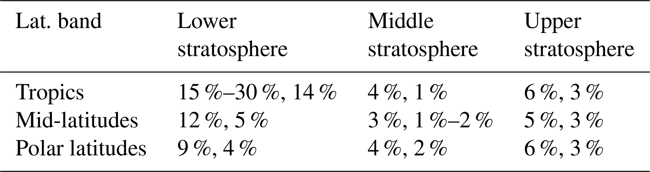
This estimation of the random uncertainty implies that each component is independent from the others. However, as discussed in Fig. 13, there is some correlation level between different error components, and it is sensible to assume that they are, to some extent, interdependent. However, not having reliable information, we assume them to be independent. The overall random uncertainty as a function of altitude and latitude is reported in Table 3 for three latitude bands in the lower, middle, and upper stratosphere in comparison with the retrieval noise component.

Table 3 Relative values of the estimated total random uncertainty due to parameter errors and retrieval noise for tropic, mid- and high latitudes, and for the lower, middle, and upper stratosphere. The first value indicates the total estimation (Eq. 11) and the second value indicates the retrieval noise component (from Fig. 1).

The systematic uncertainty includes for each altitude the following terms:

$$\begin{array}{}\text{(12)}& {\mathit{\delta }}_{x,\mathrm{systematic}}=\sqrt{{\left({\mathit{\delta }}_{x,\mathrm{unpert}}+{\mathit{\delta }}_{x,\mathrm{clouds}}+{\mathit{\delta }}_{x,\mathrm{RTM}}\right)}^{\mathrm{2}}+{\mathit{\delta }}_{x,\mathrm{cs}}^{\mathrm{2}}},\end{array}$$

where the terms with known signs are first summed up, and finally, the rms with the cross section term is performed. We do not include here the term related to the effects of changing the ozone cross section, as its choice is arbitrary and shall be evaluated on a case-by-case basis when comparing with other instruments or retrieved products.

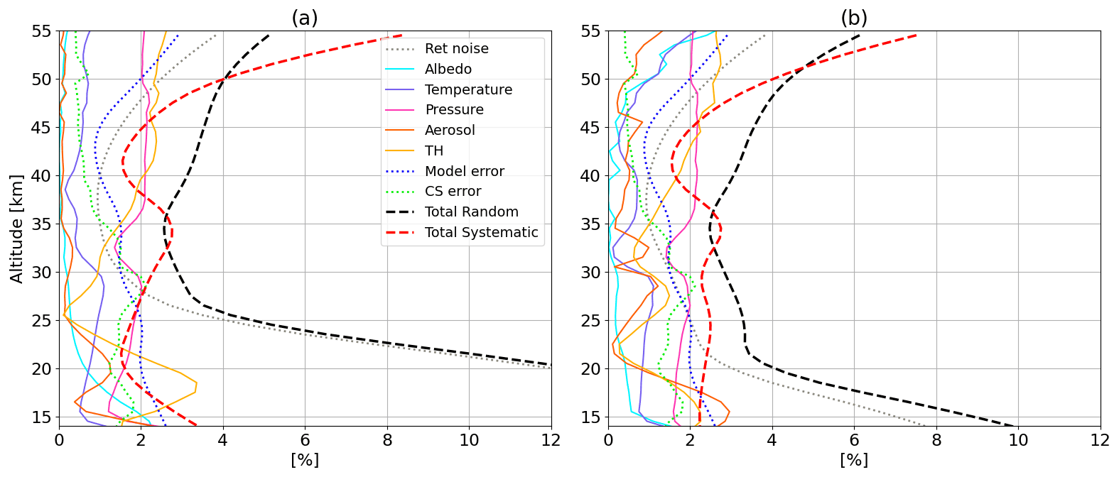
Figure 12 Contributions to the total uncertainty on ozone profiles in the tropics (a) and at high latitudes (b) in summer. The total random uncertainty is reported with the dashed black line, whereas the estimated systematic bias is shown with the red dashed line.

Figure 13 Correlation matrices between several error components for autumn. (a) Pearson correlation coefficient over latitudes at 30 km; (b) correlation coefficient for northern mid-latitudes over altitude.

Figure 12a and b display relevant uncertainty contributions for the tropics and high latitudes, respectively, for the summer season, together with the estimated total random uncertainty from Eq. (11) and the systematic bias from Eq. (12).

In compliance with the recommendations in von Clarmann et al. (2020), we also calculate correlations between relevant errors as a function of latitude, altitude, and season (not shown). Figure 13 presents an example of correlation matrices, reporting correlation coefficients over latitude and altitude for autumn. As an example, only the parameter uncertainties are here taken into consideration.

Figure 13a shows the Pearson correlation coefficients at 30 km over latitudes – i.e., it indicates how the several error components are correlated in the middle stratosphere when changing the latitude. Figure 13b shows the correlation over altitude, with low values indicating that the vertical structure of the uncertainties is different, e.g., the vertical profiles of pressure and aerosol extinction components.

One of the final goals of this study is to provide the user interested in uncertainty estimations with arrays giving the error budget as a function of altitude in 5 latitude bands and 4 seasons. In addition to these values, correlation matrices, as shown in Fig. 13, can be obtained upon request.

7.1 Verification of the uncertainties

A comparison between ex ante and ex post uncertainties (von Clarmann et al., 2020) is carried out to provide a first verification of the discussed errors. A simple test to validate the precision estimates, i.e., to prove that the retrieval noise is not under- or overestimated, is the comparison between the variance of the differences of collocated observations of the same instrument s² with the estimated uncertainty σ². In general, it is expected that

$$\begin{array}{}\text{(13)}& {\mathit{s}}^{\mathrm{2}}=\mathrm{2}\times {\mathit{\sigma }}^{\mathrm{2}}+{\mathit{\sigma }}_{x,\mathrm{nat}}^{\mathrm{2}}.\end{array}$$

Using self-collocated observations, we can assume that the term σ_x,nat, i.e., the natural atmospheric variability, approaches zero when collocation criteria become more tight, so that a direct proportionality between estimated precision and standard deviation of the collocated observations is predicted by Eq. (13). This method was followed, for example, by Piccolo and Dudhia (2007), Bourassa et al. (2012), and Sofieva et al. (2021) and is referred to as “structure functions”.

OMPS-LP is not designed to make repeated measurements of the same atmospheric scene; however, an approximation is available from the pairs of measurements located at the intersections of OMPS orbits a few hours apart. If the collocations are sufficiently close in space and time so that atmospheric variations can be neglected, the actual precision of the retrievals can be estimated from the standard deviation of these observations.

Figure 14 shows the results for OMPS-LP self-collocations with criteria Δ latitude 2^∘, Δ longitude 10^∘, and Δ time 6 h, considering observations from different orbits, i.e., avoiding matching consecutive measurements when reducing the collocation distance. In different colors, collocations within progressively shorter distances are considered, from 400 down to 100 km. The number of available collocations per year is ∼ several thousands for the widest constraints and ∼ 100 for the strictest one.

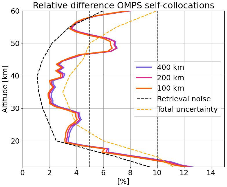
Figure 14 Relative difference between self-collocated OMPS-LP observations when changing the collocation criteria. Superimposed, typical retrieval noise and total random uncertainty for high latitudes.

As shown in the plot, the typical retrieval noise is smaller than the standard deviation of the collocated pairs. This is expected, as the precision is obtained from a linear error propagation through the RTM, whereas the retrieval process is thought to be non-linear (Piccolo and Dudhia, 2007). In addition, the standard deviation of self-collocated profiles is expected to be larger, because it includes the variability of the atmosphere, and above 40 km, diurnal variations might also play a role. On the other hand, the estimated total precision represents an upper boundary of the uncertainty for the ozone retrieval. At altitudes around 48–52 km, we notice a peak of the s² term, indicating an underestimation of the uncertainties at these altitudes.

7.2 Validation of uncertainties

To validate the total uncertainty, we used the χ² approach, applied, for example, by (Migliorini et al., 2004; von Clarmann, 2006; Steck et al., 2007). In this approach, the bias between the current dataset and collocated observations from an independent instrument (MLS in our case) is calculated as follows:

$$\begin{array}{}\text{(14)}& \mathit{b}={\displaystyle \frac{{\sum }_{n=\mathrm{1}}^K\left({\mathit{O}}_{{\mathrm{3}}_{\mathrm{OMPS},n}}-{\mathit{O}}_{{\mathrm{3}}_{\mathrm{MLS},n}}\right)}{K}},\end{array}$$

where K is the number of collocated OMPS-MLS profile pairs. The uncertainty at each altitude is then validated by comparing the de-biased mean square difference of the collocated measurements with the ex ante estimate of the total uncertainty (${\mathit{\sigma }}_x^{\mathrm{2}}$) in a χ² sense:

$$\begin{array}{}\text{(15)}& {\mathit{\chi }}^{\mathrm{2}}={\displaystyle \frac{{\sum }_{n=\mathrm{1}}^K{\left({\mathit{O}}_{{\mathrm{3}}_{\mathrm{OMPS},n}}-{\mathit{O}}_{{\mathrm{3}}_{\mathrm{MLS},n}}-\mathit{b}\right)}^{\mathrm{2}}/K}{{\mathit{\sigma }}_x^{\mathrm{2}}}},\end{array}$$

where ${\mathit{\sigma }}_x^{\mathrm{2}}$ is the sum of three squared terms:

$$\begin{array}{}\text{(16)}& {\mathit{\sigma }}_x^{\mathrm{2}}={\mathit{\sigma }}_{x,\mathrm{OMPS}}^{\mathrm{2}}+{\mathit{\sigma }}_{x,\mathrm{MLS}}^{\mathrm{2}}+{\mathit{\sigma }}_{x,\mathrm{mismatch}}^{\mathrm{2}},\end{array}$$

where σ_x,OMPS corresponds to the total random uncertainty from OMPS-LP error budget (σ_x,random in Eq. 11), σ_x,MLS is the estimated precision for MLS ozone profiles from Livesey et al. (2020), and σ_x,mismatch corresponds to expected atmospheric variability for the chosen collocation criteria. The latter has been assessed using model simulations, as described in the study by Laeng et al. (2021). The authors provided us with appropriate values of the expected atmospheric variability as function of latitude, season, and altitude. The χ² value, introduced in Eq. (15), gives an indication whether the two datasets agree with the estimated total random error.

Figure 15 In panel (a), contributing terms from Eq. (16) and de-biased rms difference between OMPS-LP and MLS (numerator of Eq. 15). In panel (b), χ² values obtained as validation metrics for the combined OMPS-LP and MLS uncertainty.

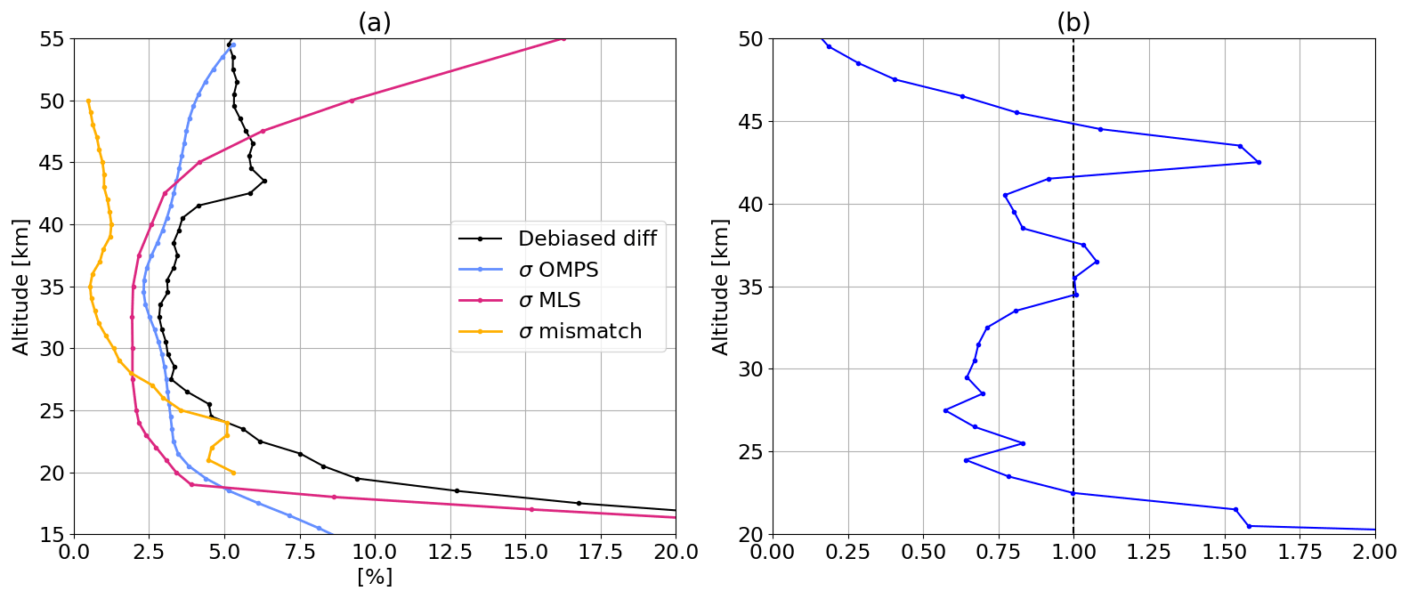
Figure 15a shows the three contributions to ${\mathit{\sigma }}_x^{\mathrm{2}}$ together with the numerator of Eq. (15), i.e., the de-biased rms difference between OMPS-LP and MLS, for mid-latitudes in autumn, as an example. The atmospheric variability profile is available only between 20 and 50 km. The right panel reports the obtained χ². Values above 1 indicate that the de-biased rms difference exceeds the estimated combined uncertainty. In our case, the ratio generally stays around 1, indicating a reasonable assessment of the combined uncertainty, at least between 20 and 45 km. However, at 42–45 km as well as below 22 km, σ_x is too small to explain the bias between the two datasets. Between 25 and 33 km, values of about 0.75 indicate a slight overestimation of the combined uncertainty, possibly from OMPS (looking at Fig. 15a). The low χ² values above 45 km indicate that the combined random uncertainty is too large in the upper stratosphere, where MLS has an associated precision that exceed 100 %. A possible overestimation of MLS errors, due to the inclusion of the smoothing error into the reported total random uncertainty, was already reported by Laeng et al. (2015).

8 Conclusions

In this paper, we presented an extensive error budget assessment for OMPS-LP ozone profiles retrieved at the University of Bremen. Synthetic simulations with the SCIATRAN RTM have been used to estimate a systematic and a random component of the uncertainty on ozone profiles. Effort has been put towards characterizing the uncertainty components and being compliant with the TUNER recommendations.

First, a retrieval bias was estimated by using unperturbed simulations and comparing them with the “true” ozone profile. This procedure highlighted a negative bias in the upper stratosphere, fairly constant with latitude, of about 5 %–8 % above 50 km. Then, parameter uncertainties were extensively investigated, and we found that the most relevant contribution is the pointing accuracy of the instrument, especially in the upper stratosphere, with values up to 3 %–4 %, followed by pressure and temperature error contributions. The precision of the retrieved aerosol extinction profiles plays a relevant role below 25 km, with a parameter uncertainty up to 4 %. The effect of an undetected cloud was also discussed and a potential negative bias in the lower stratosphere highlighted. Another relevant source of error is related to the chosen ozone cross section. It was shown that changing the cross section in the UV leads to variations of up to 2 % above 30 km in ozone. The cross section error propagated into L2 profiles is estimated to be on the order of ±2 % in the lower stratosphere; decreasing with altitude, this term has a systematic nature. In addition, the analysis of the error from model approximations revealed that the radiative transfer solver and polarization effects may add to the total random ozone error, with a contribution of up to 1 %–2 %.

Overall, most error components have shown a multiplicative nature. By summing up the single random uncertainty components and the discussed systematic errors, we provided reference values for the total uncertainty as a function of altitude and latitude. Typically, the total random uncertainty on retrieved ozone profiles is expected to lie in the range of 5 %–30 % for the lower stratosphere, 3 %–5 % for the middle stratosphere, and 5 %–7 % for the upper stratosphere. The systematic uncertainty is mainly related to cloud contamination below 20 km, producing an underestimation in the ozone profile, and to the retrieval bias above 50 km, also as underestimation of the true profile.

Uncertainties have been verified using self-collocated OMPS-LP measurements at high latitudes, finding that the standard deviation of the collocated profiles approaches the typical retrieval noise values, except at altitudes of about 28 and 50 km. The validation of the uncertainties in a χ² approach showed that the combined OMPS-LP and MLS uncertainty is reasonable but generally overestimated: a fair consistency between the combined uncertainty and the de-biased difference between the two satellites was found between 22 and 45 km, whereas in the upper stratosphere, MLS reported uncertainties are too large.