Estimates of remote sensing retrieval errors by the GRASP algorithm: application to ground-based observations, concept and validation

Understanding the uncertainties in the retrieval of aerosol and surface properties is very important for an adequate characterization of the processes that occur in the atmosphere. However, the reliable characterization of the error budget of the retrieval products is a very challenging aspect that currently remains not fully resolved in most remote sensing approaches. The level of uncertainties for the majority of the remote sensing products relies mostly on post-processing validations and intercomparisons with other data, while the dynamic errors are rarely provided. Therefore, implementations of fundamental approaches for generating dynamic retrieval errors and the evaluation of their practical efficiency remains of high importance.

This study describes and analyses the dynamic estimates of uncertainties in aerosol-retrieved properties by the GRASP (Generalized Retrieval of Atmosphere and Surface Properties) algorithm. The GRASP inversion algorithm, described by Dubovik et al. (2011, 2014, 2021), is designed based on the concept of statistical optimization and provides dynamic error estimates for all retrieved aerosol and surface properties. The approach takes into account the effect of both random and systematic uncertainties propagations. The algorithm provides error estimates both for directly retrieved parameters included in the retrieval state vector and for the characteristics derived from these parameters. For example, in the case of the aerosol properties, GRASP directly retrieves the size distribution and the refractive index that are used afterwards to provide phase function, scattering, extinction, single scattering albedo, etc. Moreover, the GRASP algorithm provides full covariance matrices, i.e. not only variances of the retrieval errors but also correlations coefficients of these errors. The analysis of the correlation matrix structure can be very useful for identifying less than obvious retrieval tendencies. This appears to be a useful approach for optimizing observation schemes and retrieval set-ups.

In this study, we analyse the efficiency of the GRASP error estimation approach for applications to ground-based observations by a sun/sky photometer and lidar. Specifically, diverse aspects of the error generations and their evaluations are discussed and illustrated. The studies rely on a series of comprehensive sensitivity tests when simulated sun/sky photometer measurements and lidar data are perturbed by random and systematic errors and inverted. Then, the results of the retrievals and their error estimations are analysed and evaluated. The tests are conducted for different observations of diverse aerosol types, including biomass burning, urban, dust and their mixtures. The study considers observations of AErosol RObotic NETwork (AERONET) sun/sky photometer measurements at 440, 675, 870 and 1020 nm and multiwavelength elastic lidar measurements at 355, 532 and 1064 nm. The sun/sky photometer data are inverted alone or together with lidar data.

The analysis shows overall successful retrievals and error estimations for different aerosol characteristics, including aerosol size distribution, complex refractive index, single scattering albedo, lidar ratios, aerosol vertical profiles, etc. Also, the main observed tendencies in the error dynamic agree with known retrieval experience. For example, the main accuracy limitations for retrievals of all aerosol types relate to the situations with low optical depth. Also, in situations with multicomponent aerosol mixtures, the reliable characterization of each component is possible only in limited situations, for example, from radiometric data obtained for low solar zenith angle observations or from a combination of radiometric and lidar data. At the same time, the total optical properties of aerosol mixtures are always retrieved satisfactorily.

In addition, the study includes an analysis of the detailed structure of the correlation matrices for the retrieval errors in mono- and multicomponent aerosols. The conducted analysis of error correlation appears to be a useful approach for optimizing observation schemes and retrieval set-ups. The application of the approach to real data is provided.

1 Introduction

Remote sensing is one major tool for monitoring atmosphere and surface properties at large scales. These observations have a nondestructive character and allow for dynamic local, regional or global monitoring of the ambient atmosphere. Correspondingly, diverse remote sensing observations are employed for routine observations and characterization of the Earth atmosphere. One of the key challenges in implementing remote sensing is the development of the retrieval algorithms. While remote sensing retrievals have substantially evolved during the last few decades, a significant need for further advancing various aspects of the retrieval algorithms remains. One of the most challenging and important, while underdeveloped, aspects is the evaluation of the errors in the retrieval products. For example, the review by Sayer et al. (2020) emphasizes that, for most aerosol satellite retrievals, the quality of the retrieval uncertainty estimates has not been routinely assessed.

Here we discuss and analyse the approach implemented in the GRASP (Generalized Retrieval of Atmosphere and Surface Properties) retrieval algorithm. The GRASP concept is based on the statistical optimization fitting designed for the retrieval of detailed aerosol properties from diverse observations (Dubovik et al., 2011, 2014, 2021). This algorithm uses statistical estimates of random error propagation and provides the dynamic error estimates for both retrieved parameters (such as the size distribution, refractive index, etc.) and characteristics derived from those parameters (total scattering, extinction, single scattering albedo, etc.). Specifically, in this work, we discuss and analyse the error estimates of the aerosol properties by GRASP for aerosol retrievals from ground-based observations by sun/sky radiometers and lidars.

One of the most visible data sets of ground-based radiometric observations is provided by AERONET (AErosol RObotic NETwork; Holben et al., 1998), a network of more than 500 operational sites distributed over the world. AERONET provides column-integrated aerosol properties of the different sites distributed over the world. AERONET provides column-integrated aerosol properties originally provided by the Nakajima et al. (1996) algorithm and later by the Dubovik and King (2000) retrieval. Several studies access the AERONET retrieval errors. First, Dubovik et al. (2000) provided a rather comprehensive analysis of retrieval uncertainties caused by both random measurement errors and systematic errors originating from potential biases in the measurements and imperfections in the modelling aerosol properties. This analysis was revisited by Torres et al. (2017), whose studies overall confirmed most of the uncertainty tendencies revealed by Dubovik et al. (2000). Recently, Sinyuk et al. (2020) published a concept for uncertainty in aerosol retrievals that have been adapted in the version 3 aerosol operational product of AERONET (Giles et al., 2019). In the frame of this concept, the uncertainties are estimated using the spread of retrieved parameters generated by 27 distinct combinations of retrieval implemented with perturbed input data (aerosol optical depth (AOD), sky radiances, solar spectral irradiance and surface reflectance). A somewhat similar concept for the estimating error was employed earlier in the LiRIC (Lidar and Radiometer Inversion Code) approach for the synergetic processing of co-located lidar and AERONET sun/sky photometer observations (Chaikovsky et al., 2016). LiRIC provided some uncertainty, which was simulated using a series of retrievals with the perturbed input data. A large number of factors affect the retrievals, whose variation is complex and nonlinear. Indeed, modelling all the factors and circumstances that can affect the retrieval in all situations is theoretically impossible, and practically challenging, within the limited series of perturbed runs, especially for situations when a large number of parameters is retrieved. In these situations, the error propagation approaches based on statistical estimation theory and described in numerous textbooks (e.g. Edie et al., 1971; Fourgeaud and Fuchs, 1967; Rodgers, 2000) provide asymptotically comprehensive estimates for random retrieval errors. At the same time, it should be noted that both the result of perturbation tests and statistical estimates of propagated error relying on the forward model employed may not fully represent the inaccuracies related to the limitations of this model. Some additional evaluations and considerations are always desirable for accessing the adequacy of the chosen forward model and its potential limitations.

The GRASP is a state-of-the-art, highly versatile inversion algorithm of a new generation that can be applied to a variety of remote sensing and laboratory observations. For example, GRASP has been applied for several satellite instruments (Dubovik et al., 2019, 2021; Li et al., 2019; Chen et al., 2018, 2019, 2020; Puthukkudy et al., 2020) and demonstrated the capability to provide accurate information about detailed properties of aerosol and underlying surface reflectance. The GRASP has been successfully used for retrieving aerosol properties from polar nephelometer data (Espinosa et al., 2017, 2019; Schuster et al., 2019). The applications of the GRASP algorithm for retrieving aerosol properties from sun/sky photometer and radiometer observations, either alone or in combination with lidar observations, have been employed and discussed in numerous studies (e.g. Torres et al., 2017) as the synergy of sun/sky photometer plus lidar (Lopatin et al., 2013, 2021; Torres et al., 2017; Benavent-Oltra et al., 2017, 2019, 2021; Hu et al., 2019; Tsekeri et al., 2017; Román et al., 2018; Herreras et al., 2019; Titos et al., 2019). The successful application of GRASP has been illustrated for the interpretation of terrestrial observations with a celestial camera (Román et al., 2017). Recent studies by Torres et al. (2017) and Torres and Fuertes (2021) demonstrated the high potential of the GRASP retrieval concept for inverting only direct sun photometric observations.

The evaluation of the retrieval accuracy in all those studies was realized by comparing and validating the retrieval results with independent reliable data. It should be noted, however, that practically none of these studies discuss the retrieval error estimates, while the formalism of the error estimate has been realized in GRASP for a while. As a result, the validity of the retrieval error estimates provided by the GRASP approach remains unattended and unverified. Therefore, in order to address this issue, the current work proposes a discussion of the main aspects of the GRASP error generation and attempts to provide an evaluation of the retrieval error estimates provided by GRASP. The study is focused on the considerations of aerosol retrieval from sun/sky photometers and lidar ground-based observations.

2 Modelling of error estimates in the GRASP algorithm

As mentioned in the introduction, in this work we make use of the GRASP (Generalized Retrieval of Atmosphere and Surface Properties) algorithm. It is a rigorous, versatile and open-source algorithm capable of providing information of aerosol properties from the measurements of different instruments and dynamic error estimates (Dubovik et al., 2011, 2014, 2021). It is a flexible, generalized algorithm that relies on two independent modules, i.e. the forward model and the numerical inversion. The forward model contains the full description of the physical model, including various interactions of electromagnetic solar radiations, such as aerosol scattering, surface reflectance and gaseous absorption. The multiple scattering interactions in the atmosphere are accounted for by solving the vector of radiative transfer equation. Thus, the GRASP forward model is capable of simulating diverse measurements in the laboratory and atmospheric remote sensing, including passive and active observations from space and the ground. On the other hand, numerical inversion is not directly related to any physical problem and realizes the formal inversion of the measurements using a statistical estimation approach. Specifically, GRASP employs the multiterm least squares method (LSM) that allows for a flexible utilization of multiple a priori constraints. This approach is very convenient for designing diverse remote sensing retrievals, as discussed in detail by Dubovik et al. (2021).

The retrieval error estimates in GRASP are calculated by modelling the propagation of measurement errors based on a statistical estimation approach. In addition, the formulation used for estimating errors accounts for some contribution of the systematic errors that could originate from biases in the measurement or some modifications implemented in the algorithm for improving the retrieval convergence of nonlinear solutions. Below, the descriptions of the overall concept and specific key implementations of the error estimation in GRASP are provided.

2.1 The numerical inversion based on a statistical optimization concept

The multiterm LSM employed in GRASP searches for the solution using statistically optimized fitting under multiple a priori constraints (Dubovik, 2004; Dubovik et al., 2011, 2021). It considers both measurements and a priori data in a similar manner by considering them as being data from different and independent data sources, as follows:

$$\begin{array}{}\text{(1)}& {\mathit{f}}_k^{*}={\mathit{f}}_k\left(\mathit{a}\right)+\mathrm{\Delta }{\mathit{f}}_k^{*},\end{array}$$

where f_k(a) is the physical forward model, a is the vector of unknown parameters, $\mathrm{\Delta }{\mathit{f}}_k^{*}$ represents the uncertainty associated with the measurement ${\mathit{f}}_k^{*}$ and k denotes different data sets that are not correlated and may have different levels of uncertainties described by different covariance matrices C_k. Such an explicit differentiation of the input data makes the retrieval more transparent because it clearly identifies the different data sets used. Correspondingly, the joint probability density function (PDF) of independent data sets ${\mathit{f}}_{\mathrm{1}}^{*}$, ${\mathit{f}}_{\mathrm{2}}^{*},\mathrm{\dots },{\mathit{f}}_K^{*}$ can be obtained by the simple multiplication of the PDFs of data from all K sources, as follows:

$$\begin{array}{}\text{(2)}& \begin{array}{rl}P\left(\mathit{f}\right(\mathit{a}\left)\right|{\mathit{f}}^{*})& =P\left({\mathit{f}}_{\mathrm{1}}\left(\mathit{a}\right),\mathrm{\dots },{\mathit{f}}_K\left(\mathit{a}\right)|{\mathit{f}}_{\mathrm{1}}^{*},\mathrm{\dots },{\mathit{f}}_K^{*}\right)\\ & =\prod _{k=\mathrm{1}}^{K}P\left({\mathit{f}}_k\right(\mathit{a}\left)\right|{\mathit{f}}_k^{*}).\end{array}\end{array}$$

It can be noted that Eq. (1) does not assume any relation between the forward models f_k(a), i.e. forward models f_k(a) can be the same or different. In the frame of the LSM approach, i.e. under the assumptions of a normal PDF of the error $\mathrm{\Delta }{\mathit{f}}_k^{*}$, the solution of the Eq. (1) corresponds to the minimum of the following functional:

$$\begin{array}{}\text{(3)}& \mathrm{2}\widehat{\mathrm{\Psi }}\left(\mathit{a}\right)={\displaystyle \frac{\mathrm{1}}{\mathrm{2}}}\sum _{k=\mathrm{1}}^K\left({\mathit{f}}_k\right(\mathit{a})-{\mathit{f}}_k^{*}{)}^T{\mathbf{C}}_k^{-\mathrm{1}}({\mathit{f}}_k\left(\mathit{a}\right)-{\mathit{f}}_k^{*})=min.\end{array}$$

It can be noted that, if any of correlation coefficients are 1 or −1, the covariance matrix is degenerated with det(C_k)=0.

For the general case of nonlinear functions f_k(a), the solution of Eq. (3) is sought iteratively, as follows:

$$\begin{array}{}\text{(4)}& {\mathit{a}}^{p+\mathrm{1}}={\mathit{a}}^p-\mathrm{\Delta }{\mathit{a}}^p,\end{array}$$

where Δa^p is the solution that can be found by solving the system of so-called normal equations. This is as follows:

$$\begin{array}{}\text{(5)}& \left(\sum _{k=\mathrm{1}}^K{\mathbf{K}}_{k,p}^T{\mathbf{C}}_k^{-\mathrm{1}}{\mathbf{K}}_{k,p}\right)\mathrm{\Delta }{\mathit{a}}^p=\sum _{k=\mathrm{1}}^K{\mathbf{K}}_{k,p}^T{\mathbf{C}}_k^{-\mathrm{1}}\mathrm{\Delta }{\mathit{f}}_k^p,\end{array}$$

where $\mathrm{\Delta }{\mathit{f}}^p=\mathit{f}\left({\mathit{a}}^p\right)-{\mathit{f}}^{*}$, and K_p is a Jacobean matrix at the pth iteration of the functions f_k(a) in the vicinity of a^p with the elements ${\left\{{\mathbf{K}}_{k,p}\right\}}_{j,i}={\left.\frac{\partial {\mathit{f}}_{k,j}\left(\mathit{a}\right)}{\partial {\mathrm{a}}_i}\right|}_{\mathit{a}={\mathit{a}}^p}$.

The asymptotic limit of the minimized quadratic form, for most applications, can be written as follows:

$$\begin{array}{}\text{(6)}& \mathrm{2}\mathrm{\Psi }\left(\mathit{a}\right)=min\to \sum _{k=\mathrm{1}}^K{N}_k-n,\end{array}$$

where N_k is a number of measurements (inputs) in the kth data set, and n is the number of retrieved unknowns (parameters).

It should be noted that the LSM solution of Eq.(3) corresponds to the minimum of the quadratic form $\widehat{\mathrm{\Psi }}\left(\mathit{a}\right)$ and does not depend on the value of this minimum. Considering this fact, in a practical application it is often convenient to renormalize the minimized quadratic $\widehat{\mathrm{\Psi }}\left(\mathit{a}\right)$, and in situations when only one data set is inverted, it is convenient to use a weighting matrix $\mathbf{W}=\mathbf{C}/{\mathit{\epsilon }}_{\mathrm{1}}^{\mathrm{2}}$ and minimize the quadratic form $\mathrm{2}{\mathrm{\Psi }}^{\prime }\left(\mathit{a}\right)=\mathrm{2}{\mathit{\epsilon }}_{\mathrm{1}}^{\mathrm{2}}\mathrm{\Psi }\left(\mathit{a}\right)$. In such an approach, one does not need to know the exact value of the variance ${\mathit{\epsilon }}_{\mathrm{1}}^{\mathrm{2}}$. Moreover, ${\mathit{\epsilon }}_{\mathrm{1}}^{\mathrm{2}}$ can be estimated from asymptotic LSM expectations provided by Eq. (9), as shown below.

In the frame of a multiterm approach, the use of weighting matrices additionally allows for making the contribution of different data sources more explicit. Indeed, using the weighting matrices W_k instead of covariance matrices C_k in Eq. (5) can be written as follows:

$$\begin{array}{}\text{(7)}& \left(\sum _{k=\mathrm{1}}^K{\mathit{\gamma }}_k{\mathbf{K}}_k^T{\mathbf{W}}_k^{-\mathrm{1}}{\mathbf{K}}_k\right)\mathrm{\Delta }{\mathit{a}}^p=\sum _{k=\mathrm{1}}^K{\mathit{\gamma }}_k{\mathbf{K}}_k^T{\mathbf{W}}_k^{-\mathrm{1}}\mathrm{\Delta }{\mathit{f}}_k^p.\end{array}$$

In this formulation, the relative contributions of the data from different data sources are scaled by the corresponding Lagrange parameters, γ_i, defined as follows:

$$\begin{array}{}\text{(8)}& {\mathbf{W}}_i={\displaystyle \frac{\mathrm{1}}{{\mathit{\epsilon }}_i^{\mathrm{2}}}}{\mathbf{C}}_i\text{and}{\mathit{\gamma }}_i={\displaystyle \frac{{\mathit{\epsilon }}_{\mathrm{1}}^{\mathrm{2}}}{{\mathit{\epsilon }}_i^{\mathrm{2}}}},\end{array}$$

where ${\mathit{\epsilon }}_i^{\mathrm{2}}$ is the first diagonal element of C_i, i.e.  ${\mathit{\epsilon }}_i^{\mathrm{2}}=\mathit{\{}{\mathbf{C}}_i{\mathit{\}}}_{\mathrm{11}}$, and γ_i is the ratio of the variances of scattered radiances and variances of the corresponding data set. Evidently, γ₁=1, as discussed by Dubovik and King (2000); Dubovik (2004); Dubovik et al. (2011) and others. This renormalization strategy is especially convenient for a multiterm LSM approach once some of data sets correspond to a priori information. In addition, the renormalized definition of the minimized quadratic function (or residual) is ${\mathrm{\Psi }}^{\prime }\left(\mathit{a}\right)={\mathit{\epsilon }}_{\mathrm{1}}^{\mathrm{2}}\mathrm{\Psi }\left(\mathit{a}\right)$, and the measurement error variance ${\mathit{\epsilon }}_{\mathrm{1}}^{\mathrm{2}}$ can be estimated from the residual of the fit. Indeed, once the weighting matrices are used in the solution, and taking into account that the values of minimized quadratic form of $\mathrm{\Psi }\left(\widehat{\mathit{a}}\right)$ follow a χ² distribution, Eq. (7) minimizes the quadratic form with the limit depending on ${\mathit{\epsilon }}_{\mathrm{1}}^{\mathrm{2}}$, as follows:

$$\begin{array}{}\text{(9)}& \begin{array}{rl}& \mathrm{2}{\mathrm{\Psi }}^{\prime }\left(\mathit{a}\right)=\mathrm{2}{\mathit{\epsilon }}_{\mathrm{1}}^{\mathrm{2}}\mathrm{\Psi }\left(\mathit{a}\right)=min\to {\mathit{\epsilon }}_{\mathrm{1}}^{\mathrm{2}}\left(\sum _{k=\mathrm{1}}^K{N}_k-n\right)\\ & \text{and}{\widehat{\mathit{\epsilon }}}_{\mathrm{1}}^{\mathrm{2}}\approx {\displaystyle \frac{\mathrm{2}{\mathrm{\Psi }}^{\prime }\left({\mathit{a}}^p\right)}{{\sum }_{k=\mathrm{1},\mathrm{\dots },K}{N}_k-n}}.\end{array}\end{array}$$

Therefore, ${\mathit{\epsilon }}_{\mathrm{1}}^{\mathrm{2}}$ can be estimated from the minimum value of the residual $\mathrm{\Psi }\left(\widehat{\mathit{a}}\right)$.

A priori constraints in a multiterm LSM approach and in GRASP algorithm

As discussed in detail by Dubovik et al. (2021), the multiterm LSM concept has been proposed as being a methodologically convenient approach for integrating different types of a priori constraints in remote sensing applications (Dubovik, 2004; Dubovik and King, 2000; Dubovik et al., 1995, 2000, 2008, 2011). In the multiterm LSM, a priori estimates are considered to be equivalent to the measurements, i.e. characterized by their PDF and treated equivalently to the actual measurements. In this regard, Eqs. (1)–(7) do not show any distinction between different f_k(a).

At the same time, in practice, there are always two different types of data sets, i.e. measurements and the a priori constraint on the unknowns a. Therefore, the vector of the measurement $({\mathit{f}}^{*}{)}^T=({\mathit{f}}_{\mathrm{1}}^{*},{\mathit{f}}_{\mathrm{2}}^{*},\mathrm{\cdots },{\mathit{f}}_K^{*}{)}^T$ can be written as follows:

$$\begin{array}{}\text{(10)}& ({\mathit{f}}^{*}{)}^T=({\mathit{f}}_{\mathrm{1}}^{*},{\mathit{f}}_{\mathrm{2}}^{*},\mathrm{\dots },{\mathit{f}}_K^{*},{\mathit{f}}_{\mathrm{1}}^{\mathrm{a}},{\mathit{f}}_{\mathrm{2}}^{\mathrm{a}},\mathrm{\dots },{\mathit{f}}_N^{\mathrm{a}}{)}^T,\end{array}$$

where ${\mathit{f}}_i^{*}={\mathit{f}}_i^{*}\left(\mathit{a}\right)$ represent K directly measured characteristics, and ${\mathit{f}}_i^{\mathrm{a}}={\mathit{f}}_i^{\mathrm{a}}\left(\mathit{a}\right)$ represent N a priori known characteristics of unknowns a. Correspondingly, the right-hand side of Eq. (2) can be formally split into the following two groups:

$$\begin{array}{}\text{(11)}& P\left(\mathit{f}\right(\mathit{a}\left)\right|{\mathit{f}}^{*})=\prod _{k=\mathrm{1}}^{K}P({\mathit{f}}_k\left(\mathit{a}\right)\left|{\mathit{f}}_k^{*}\right)\prod _{n=\mathrm{1}}^{N}P\left({\mathit{f}}_n^{\mathrm{a}}\right(\mathit{a}\left)\right|{\mathit{f}}_n^{\mathrm{a},*}).\end{array}$$

Therefore, Eq. (7) can also be formally arranged to identify the contribution of measurements and a priori terms, as follows:

$$\begin{array}{}\text{(12)}& \begin{array}{rl}(\sum _{k=\mathrm{1}}^K{\mathit{\gamma }}_k{\mathbf{K}}_{k,p}^T{\mathbf{W}}_k^{-\mathrm{1}}{\mathbf{K}}_{k,p}& +\sum _{n=\mathrm{1}}^N{\mathit{\gamma }}_{\mathrm{a},n}{\mathbf{K}}_{\mathrm{a},n,p}^T{\mathbf{W}}_{\mathrm{a},n}^{-\mathrm{1}}{\mathbf{K}}_{\mathrm{a},n,p})\mathrm{\Delta }{\mathit{a}}^p\\ & =\sum _{k=\mathrm{1}}^K{\mathit{\gamma }}_k{\mathbf{K}}_{k,p}^T{\mathbf{W}}_k^{-\mathrm{1}}\mathrm{\Delta }{\mathit{f}}_k^{*,p}\\ & +\sum _{n=\mathrm{1}}^N{\mathit{\gamma }}_{\mathrm{a},n}{\mathbf{K}}_{\mathrm{a},n,p}^T{\mathbf{W}}_{\mathrm{a},n}^{-\mathrm{1}}\mathrm{\Delta }{\mathit{f}}_n^{{\mathrm{a}}^{*},p},\end{array}\end{array}$$

where the two groups of the terms on left and right parts of the equation represent the contributions of the set of K measured characteristics f_k(a) and the set of N a priori ${\mathit{f}}_n^{\mathrm{a}}\left(\mathit{a}\right)$ characteristics, and the Lagrangian parameters are defined as follows:

$$\begin{array}{}\text{(13)}& {\mathit{\gamma }}_k={\displaystyle \frac{{\mathit{\epsilon }}_{k=\mathrm{1}}^{\mathrm{2}}}{{\mathit{\epsilon }}_k^{\mathrm{2}}}}\text{and}{\mathit{\gamma }}_{\mathrm{a},n}={\displaystyle \frac{{\mathit{\epsilon }}_{n=\mathrm{1}}^{\mathrm{2}}}{{\mathit{\epsilon }}_{a,n}^{\mathrm{2}}}}.\end{array}$$

As discussed by Dubovik (2004) and Dubovik et al. (2021), the multiterm approach is a simple rearranging of the base LSM formulation, while the resulting Eq. (7) provides a solid basis for unifying many known formulas of the constrained inversion in a single formalism and is practical, convenient and efficient for developing remote sensing algorithms using diverse complementary observations and a priori constraints.

While the multiterm LSM concept allows flexible utilizations of nearly arbitrary a priori constraints, the GRASP algorithm is fully adapted for using the most popular and physically transparent a priori constraints, such as direct a priori estimates of unknowns a and smoothness constraints in situations when the unknown vector a or any group of unknowns included in this vector represent continuous smooth function. For example, if vector a represents an aerosol size distribution that is known to be rather smooth, the system given by Eq. (1) can be explicitly written as follows:

$$\begin{array}{}\text{(14)}& \begin{array}{rl}\left\{\begin{array}{rl}& {\mathit{f}}_{k=\mathrm{1}}^{*}={\mathit{f}}_{k=\mathrm{1}}^{*}\left(\mathit{a}\right)+\mathrm{\Delta }{\mathit{f}}_{k=\mathrm{1}}^{*}\\ & {\mathit{f}}_{n=\mathrm{1}}^{\mathrm{a},*}={\mathit{f}}_{n=\mathrm{1}}^{\mathrm{a},*}\left(\mathit{a}\right)+\mathrm{\Delta }{\mathit{f}}_{n=\mathrm{1}}^{\mathrm{a},*}\\ & {\mathit{f}}_{n=\mathrm{2}}^{\mathrm{a},*}={\mathit{f}}_{n=\mathrm{2}}^{\mathrm{a},*}\left(\mathit{a}\right)+\mathrm{\Delta }{\mathit{f}}_{n=\mathrm{2}}^{\mathrm{a},*}\end{array}\right.& =\left\{\begin{array}{rl}& {\mathit{f}}_{\mathrm{1}}^{*}={\mathit{f}}_{k=\mathrm{1}}^{*}\left(\mathit{a}\right)+\mathrm{\Delta }{\mathit{f}}_{\mathrm{1}}^{*}\\ & {\mathit{f}}_{\mathrm{1}}^{\mathrm{a},*}={\mathit{f}}_{\mathrm{1}}^{\mathrm{a},*}\left(\mathit{a}\right)+\mathrm{\Delta }{\mathit{f}}_{\mathrm{1}}^{\mathrm{a},*}\\ & {\mathit{f}}_{\mathrm{2}}^{\mathrm{a},*}={\mathit{f}}_{\mathrm{2}}^{\mathrm{a},*}\left(\mathit{a}\right)+\mathrm{\Delta }{\mathit{f}}_{\mathrm{2}}^{\mathrm{a},*}\end{array}\right.\\ & =\left\{\begin{array}{rl}& {\mathit{f}}_{\mathrm{1}}^{*}={\mathit{f}}_{k=\mathrm{1}}^{*}\left(\mathit{a}\right)+\mathrm{\Delta }{\mathit{f}}_{\mathrm{1}}^{*}\\ & {\mathit{a}}^{*}=\mathit{a}+{\mathrm{\Delta }}_{{\mathit{a}}^{*}}\\ & {\mathbf{0}}^{*}={\mathbf{G}}_m^{\mathit{a}}+{\mathrm{\Delta }}_{{\mathbf{g}}^{*}}.\end{array}\right.\end{array}\end{array}$$

The a priori constraints defined by the second line ${\mathit{a}}^{*}=\mathit{a}+{\mathrm{\Delta }}_{{\mathit{a}}^{*}}$ represent the most common constraints of the solution by direct a priori estimates of unknowns a^*, where ${\mathrm{\Delta }}_{{\mathit{a}}^{*}}$ are the uncertainties in the estimates a^* and are generally considered to be unbiased random errors within the covariance matrix ${\mathbf{C}}_{{\mathit{a}}^{*}}$. These constraints can be easily included in Eq. (12) by defining the K_a=1 unity matrix, i.e.  ${\mathbf{K}}_{\mathrm{a}}^T{\mathbf{W}}_{\mathrm{a}}^{-\mathrm{1}}{\mathbf{K}}_{\mathrm{a}}={\mathbf{W}}_{\mathrm{a}}^{-\mathrm{1}}$ and ${\mathbf{K}}_{\mathrm{a}}^T{\mathbf{W}}_{\mathrm{a}}^{-\mathrm{1}}{\mathit{f}}_{\mathrm{1}}^{\mathrm{a},*}={\mathbf{W}}_{\mathrm{a}}^{-\mathrm{1}}\mathit{a}$. The utilization of a priori estimates a^* was introduced in the pioneering studies by Twomey (1963) and later evolved and discussed in detail in the Rodgers (2000) textbook on inversion. The third line represents another common type of a priori constraint known as the smoothness constraints that limit the variability in retrieved functions by using a priori knowledge about limitations on derivatives of those functions. For example, a priori knowledge limits high-frequency variations in continuous functions v(x), such as the aerosol size distribution. In GRASP, the smoothness constraints are related to a priori known limited values of the derivatives, i.e. with their mth derivative deviations from zero, as follows:

$$\begin{array}{}\text{(15)}& {\displaystyle \frac{{\partial }^{m}v\left(x\right)}{\partial x^m}}\approx \mathrm{0}.\end{array}$$

For the vector of unknowns $\mathit{a}=({\mathrm{a}}_{\mathrm{1}},{\mathrm{a}}_{\mathrm{2}},\cdot ,{\mathrm{a}}_n{)}^T$ that contain discrete elements describing the continuous function v(x), the knowledge on the smoothness of function v(x) can be defined using a vector–matrix linear system (e.g. see Dubovik et al., 2021). ${\mathbf{0}}^{*}={\mathbf{G}}_m^{\mathit{a}}+{\mathrm{\Delta }}_{{\mathbf{g}}^{*}}$, where G_m is the Jacobean matrix of the matrix of the mth derivatives ${\mathbf{G}}_m^{\mathit{a}}$. In practice, these are often approximated by matrices of the mth finite difference estimated in point a. The errors ${\mathrm{\Delta }}_{{\mathbf{g}}^{*}}$ reflect the uncertainty in the knowledge of the deviations of y(x) from the assumed constant (m=1), straight line (m=2), parabola (m=3) and so on. Under the assumption that the ${\mathrm{\Delta }}_{{\mathbf{g}}^{*}}$ have a normal distribution, with mean zero and covariance matrix C_g, these constraints can be easily included in Eq. 12 by defining ${\mathbf{K}}_{\mathrm{a},\mathrm{2}}={\mathbf{G}}_m$ and ${\mathit{f}}_{\mathrm{2}}^{\mathrm{a},*}={\mathbf{0}}^{*}$, i.e.  ${\mathbf{K}}_{\mathrm{a}}^T{\mathbf{W}}_{\mathrm{a}}^{-\mathrm{1}}{\mathbf{K}}_{\mathrm{a}}={\mathbf{G}}_m^T{\mathbf{W}}_{\mathrm{\Delta }g}^{-\mathrm{1}}{\mathbf{G}}_m^T$ and ${\mathbf{K}}_{\mathrm{2}}^T{\mathbf{W}}_{\mathrm{2}}^{-\mathrm{1}}\mathrm{\Delta }{\mathit{f}}_{\mathrm{2}}^{\mathrm{a},*}={\mathbf{G}}_m^T{\mathbf{W}}_{\mathrm{\Delta }g}^{-\mathrm{1}}({\mathit{a}}^p-{\mathbf{0}}^{*})={\mathbf{G}}_m^T{\mathbf{W}}_{\mathrm{\Delta }g}^{-\mathrm{1}}{\mathit{a}}^p$. Utilization of such smoothness constraints was suggested by one of the first formulations of constrained inversion by Phillips (1962) and was also considered in an article by Tikhonov (1963) and his later studies.

Thus, for a case where only direct a priori estimates and smoothness constraints are used, Eq. (12) can be explicitly written via weighting matrices as follows:

$$\begin{array}{}\text{(16)}& \begin{array}{rl}& \left({\mathbf{K}}^T{\mathbf{W}}_f^{-\mathrm{1}}\mathbf{K}+{\mathit{\gamma }}_{\mathrm{a}}{\mathbf{W}}_{\mathrm{a}}^{-\mathrm{1}}+{\mathit{\gamma }}_g{\mathbf{\Omega }}_m\right)\mathrm{\Delta }{\mathit{a}}^p\\ & ={\mathbf{K}}^T{\mathbf{W}}_f^{-\mathrm{1}}\mathrm{\Delta }{\mathit{f}}^p+{\mathit{\gamma }}_{\mathrm{a}}{\mathbf{W}}_{\mathrm{a}}^{-\mathrm{1}}({\mathit{a}}^p-{\mathit{a}}^{*})+{\mathit{\gamma }}_g{\mathbf{\Omega }}_m{\mathit{a}}^p,\end{array}\end{array}$$

where Ω_m denotes the smoothness matrix. This is defined as follows:

$$\begin{array}{}\text{(17)}& {\mathbf{G}}_m^T{\mathbf{W}}_{\mathrm{\Delta }g}^{-\mathrm{1}}{\mathbf{G}}_m^T={\mathbf{\Omega }}_m,\end{array}$$

and the explicit formulation of Ω_m can be found in the paper by Dubovik et al. (2011). Equation (14) generalizes the commonly used base equations of constrained inversion by Phillips (1962), Twomey (1975, 1977), Tikhonov (1963) and Rodgers (1976, 1990, 2000). It should be noted that Eq. (14) is written for the simplest situation, when the vector a represents only one continuous function v(x), while, in many GRASP applications, the vector of unknowns includes several components ${\mathit{a}}^T=({\mathit{a}}_{\mathrm{sd}}^T,{\mathit{a}}_{n\left(\mathit{\lambda }\right)}^T,{\mathit{a}}_{k\left(\mathit{\lambda }\right)}^T,{\mathit{a}}_h^T,\mathrm{\dots }{)}^T$, where each component is relevant to continuous functions representing such physical characteristics as the aerosol particle size distribution (a_sd), spectral dependence of real (a_n(λ)) and complex (a_k(λ)) parts of refractive index, vertical distribution (a_h), etc. Each of those characteristics is continuous function and therefore, in retrieval, the smoothness constraints can be applied on each of corresponding component of the vector of unknowns. Evidently, direct a priori constraints can be applied to each single element of the vector a, while, from a practical viewpoint, separating and outlining the contribution of a priori estimates for each component, e.g. $({\mathit{a}}^{*}{)}^T=(({\mathit{a}}_{\mathrm{sd}}^{*}{)}^T,({\mathit{a}}_{n\left(\mathit{\lambda }\right)}^{*}{)}^T,({\mathit{a}}_{k\left(\mathit{\lambda }\right)}^{*}{)}^T,({\mathit{a}}_h^{*}{)}^T,\mathrm{\dots }{)}^T$. Similarly, the inverted measurements may come from different sources and therefore have different levels of accuracy and different weighting matrices. As a result, in practice, all the first, second and third terms in Eq. (14) may have many quite different components, and therefore, the actual formulation of the solution can be significantly more complex. Some of the explicit equations can be found in the paper by Dubovik et al. (2011).

The realization of the inversion in GRASP, in principle, is based on the general Eq. (7), while for convenience there is a logical separation, as indicated in Eq. (12), into actual measurements and a priori constraints. For each measurement data set ${\mathit{f}}_k^{*}$, two types of errors can be set, i.e. the relative or absolute, and the magnitude of the errors is defined by the standard deviation and a weighting matrix W_i. The standard deviation is used inside the code to calculate the corresponding Lagrange parameters γ_i. The weighting matrix W_i is assumed as being the unity matrix by default, while it can also be set as diagonal, with different values at the diagonal, and in a more general way with non-zero non-diagonal values too. For applying the a priori constraints, as discussed above, there are two main possibilities, namely using direct a priori constraints or applying smoothness constraints for the parameters that define continuous functions.

The direct a priori estimates ${\mathrm{a}}_i^{*}$ for each of value a_i in the vector of unknowns $\mathit{a}=({\mathrm{a}}_{\mathrm{1}},{\mathrm{a}}_{\mathrm{2}},\mathrm{\dots },{\mathrm{a}}_n{)}^T$ can be provided with the corresponding Lagrangian parameters ${\mathit{\gamma }}_{{\mathrm{a}}_i}$. There is also a possibility of assuming a vector a^* of a priori estimates for all the retrieved parameters or for selected groups (e.g. parameters describing size distribution) with the common Lagrangian parameter γ_a. In this case, the weighting matrix W_a is also provided that is assumed to be the unity matrix by default, or it can be set as diagonal, with different values at the diagonal, or in more general way with non-zero non-diagonal values.

The smoothness a priori constraints can be applied for each group of parameters describing a continuous function (e.g. ${\mathit{a}}_{\mathrm{sd}}^T,{\mathit{a}}_{n\left(\mathit{\lambda }\right)}^T,{\mathit{a}}_{k\left(\mathit{\lambda }\right)}^T,{\mathit{a}}_h^T,\mathrm{\dots }$) by defining the order m of limited derivatives (m=0 is a constant; m=1 is a straight line; m=2 is a parabola, etc.), and the strength of the applied a priori smoothness constraints is defined by Lagrangian parameters γ_n. The smoothness matrix Ω_m is defined as in Eq. (15), where the weighting matrix W_Δg is the unity matrix by default and can be set as diagonal with different values on the diagonal in case the retrieved continuous function has a different level of variability for different ordinates.

It should be noted that GRASP considers two types of a priori constraints, namely the single-pixel a priori constraints for the retrieved parameters that correspond to simultaneous and co-located observations, and the multipixel constraints that limit the variability for unknowns in different groups of similar parameters when several such groups of unknowns are retrieved simultaneously from coordinated but not fully coincident or not fully co-located observations (see details in Dubovik et al., 2011, 2021). In the current paper, only single-pixel constraints are used.

2.2 Nonlinear inversion in GRASP using the Levenberg–Marquardt optimization

Since most of atmospheric remote sensing applications are strongly nonlinear, the Levenberg–Marquardt optimization (Press et al., 1992; Ortega and Rheinboldt, 1970) is realized to optimize the convergence of GRASP solutions. Specifically, as described by Dubovik et al. (2021), in GRASP it is assumed that the correction of the solution at the pth iteration Δa^p should be limited, especially at the initial iterations when the linearization error is the largest. For such cases, in GRASP, for the determination of Δa^p in the iterative procedure, an additional constraint on the correction Δa^p is added at each iteration, as follows:

$$\begin{array}{}\text{(18)}& \mathrm{\Delta }{\mathit{a}}^{p,*}={\mathbf{0}}^{*}+\mathrm{\Delta }\mathit{a}.\end{array}$$

Correspondingly, using this additional requirement, an additional term will be introduced in Eq. (7), as follows:

$$\begin{array}{}\text{(19)}& \begin{array}{rl}& \left(\sum _{k=\mathrm{1}}^K{\mathit{\gamma }}_k{\mathbf{K}}_k^T({\mathbf{W}}_k{)}^{-\mathrm{1}}{\mathbf{K}}_k+{\mathbf{D}}_{\mathrm{\Delta }\mathit{a}}^p\right)\mathrm{\Delta }{\mathit{a}}^p\\ & =\sum _{k=\mathrm{1}}^K{\mathit{\gamma }}_k{\mathbf{K}}_k^T({\mathbf{W}}_k{)}^{-\mathrm{1}}\mathrm{\Delta }{\mathit{f}}_k^p,\end{array}\end{array}$$

where the matrix D_Δa is a diagonal matrix. This has the following elements:

$$\begin{array}{}\text{(20)}& {{\mathbf{D}}_{\mathrm{\Delta }\mathit{a}}}_{ii}={\mathit{\gamma }}_{\mathrm{\Delta }{\mathit{a}}_i}={\displaystyle \frac{{\mathit{\epsilon }}_{\mathrm{1}}^{\mathrm{2}}}{{\mathit{\epsilon }}_{\mathrm{\Delta }{\mathit{a}}_i}^{\mathrm{2}}}}.\end{array}$$

The variance ${\mathit{\epsilon }}_{\mathrm{\Delta }{\mathit{a}}_i}$ can be determined, for example, assuming that whole known range of each parameter a_i variability should be covered by $\mathrm{3}{\mathit{\epsilon }}_{\mathrm{\Delta }{\mathit{a}}_i}$, i.e. ${\mathit{a}}_{i,max}-{\mathit{a}}_{i,min}\approx \mathrm{3}{\mathit{\epsilon }}_{\mathrm{\Delta }{\mathit{a}}_i}$.

Also, following the common Levenberg–Marquardt procedure, the impact of the correction Δa^p is always scaled by a factor t_p in Eq. (4), as follows:

$$\begin{array}{}\text{(21)}& {\mathit{a}}^{p+\mathrm{1}}={\mathit{a}}^p-t_p\mathrm{\Delta }{\mathit{a}}^p,\end{array}$$

where t_p is in the range $\mathrm{0}<t_p\le \mathrm{1}$. It is selected empirically to provide convergence, by decreasing $t_p=t_p/\mathrm{2}$, until the decrease in the residual ${\mathrm{\Psi }}^{\prime }\left({\mathit{a}}^p\right)\le {\mathrm{\Psi }}^{\prime }\left({\mathit{a}}^{p-\mathrm{1}}\right)$ is achieved (see Dubovik et al., 2011).

Thus, in the case of nonlinear f_k(a) and/or ${\mathit{f}}_i^{\mathrm{a}}\left(\mathit{a}\right)$, the inversion in GRASP includes Levenberg–Marquardt-like optimizations and is implemented in the frame of Eqs. (4) and (5). While this optimization certainly helps to achieve a successful convergence of the solution in practice, it should also be considered to be one of possible sources of uncertainties, as pointed out by Dubovik et al. (2021), and will be discussed below.

2.3 Error propagation estimates in GRASP

Estimations of the retrieval errors in GRASP are based on LSM equations expressed for the case of multiterm solutions written via weighting matrixes (Dubovik et al., 2021). Both the contribution of random and systematic error components are estimated as follows:

$$\begin{array}{}\text{(22)}& {\mathbf{C}}_{\widehat{\mathit{a}}}={\mathbf{C}}_{\mathrm{\Delta }{\widehat{\mathit{a}}}_{\left(\mathrm{ran}\right)}}+\left({\widehat{\mathit{a}}}_{\mathrm{bias}}\right)({\widehat{\mathit{a}}}_{\mathrm{bias}}{)}^T,\end{array}$$

where, in the following,

$$\begin{array}{}\text{(23)}& \begin{array}{rl}{\mathbf{C}}_{\mathrm{\Delta }{\widehat{\mathit{a}}}_{\left(\mathrm{ran}\right)}}& =<\mathrm{\Delta }{\widehat{\mathit{a}}}_{\left(\mathrm{ran}\right)}\mathrm{\Delta }{\widehat{\mathit{a}}}_{\left(\mathrm{ran}\right)}^T>\\ & \approx {\left(\sum _{k=\mathrm{1}}^K{\mathit{\gamma }}_k{\mathbf{K}}_k^T{\mathbf{W}}_k^{-\mathrm{1}}{\mathbf{K}}_k\right)}^{-\mathrm{1}}{\widehat{\mathit{\epsilon }}}_{\mathrm{1}}^{\mathrm{2}}\end{array}\end{array}$$

$$\begin{array}{}\text{(24)}& \begin{array}{rl}{\widehat{\mathit{a}}}_{\mathrm{bias}}=& {\left(\sum _{k=\mathrm{1}}^K{\mathit{\gamma }}_k\left({\mathbf{K}}_k^T{\mathbf{W}}_k^{-\mathrm{1}}{\mathbf{K}}_k\right)\right)}^{-\mathrm{1}}\\ & \left(\sum _{k=\mathrm{1}}^K{\mathit{\gamma }}_k\left({\mathbf{K}}_k^T{\mathbf{W}}_k^{-\mathrm{1}}{\mathit{b}}_k^{*}\right)\right),\end{array}\end{array}$$

where ${\mathit{b}}_k^{*}$ denotes the bias vector in the kth data set f_k, and ${\widehat{\mathit{\epsilon }}}_{\mathrm{1}}^{\mathrm{2}}$ is estimated from the resulting misfit of the data using Eq. (9).

The estimation of not only the random retrieval error but also the error retrieval bias a_bias is important for the adequate evaluation of retrieval uncertainty, especially in the case when multiple a priori constraints are used. For example, for the case of the retrieval given by Eq. (14), ${\mathbf{C}}_{\mathrm{\Delta }{\widehat{\mathit{a}}}_{\mathrm{ran}}}$ is expressed as follows:

$$\begin{array}{}\text{(25)}& {\mathbf{C}}_{\mathrm{\Delta }{\widehat{\mathit{a}}}_{\mathrm{ran}}}\approx {\left({\mathbf{K}}^T{\mathbf{W}}^{-\mathrm{1}}\mathbf{K}+{\mathit{\gamma }}_{\mathit{a}}{\mathbf{W}}_{\mathit{a}}^{-\mathrm{1}}+{\mathit{\gamma }}_g{\mathbf{\Omega }}_m\right)}^{-\mathrm{1}}{\widehat{\mathit{\epsilon }}}_{\mathrm{1}}^{\mathrm{2}}.\end{array}$$

A rather obvious tendency can be seen from the analysis of this equation because the higher the contributions of the second and the third terms, the smaller the random errors are, i.e. the stronger a priori constraints used, the lower the random errors will be in the retrieval. However, in practice, a priori constraints can be unintentionally inadequate and therefore introduce some systematic uncertainties, i.e. biases. In principle, there is no guaranteed approach for detecting those biases unless a comprehensive analysis and validation of the retrievals have been done. Nonetheless, some biases can manifest themselves via misfit of measurements $\mathrm{\Delta }{\mathit{f}}_k^{\mathrm{bias}}={\mathit{f}}_k\left({\mathit{a}}^{\mathrm{solution}}\right)-{\mathit{f}}_k^{*}$ or the misfit of a priori constraints. For example, for Eq. (14), the bias can be introduced by a priori estimate ${\mathit{a}}_{\mathrm{bias}}^{*}={\mathit{a}}^{\mathrm{solution}}-{\mathit{a}}^{*}$ or unsmoothed features in the retrieved solution, i.e. ${\mathit{a}}_{\mathrm{bias}}^{\mathrm{smooth}}={\mathbf{\Omega }}_m{\mathit{a}}^{\mathrm{solution}}\ne \mathbf{0}$. Correspondingly, the bias for single-pixel retrieval is estimated as follows:

$$\begin{array}{}\text{(26)}& \begin{array}{rl}{\widehat{\mathit{a}}}_{\mathrm{bias}}\approx & {\left({\mathbf{K}}^T{\mathbf{W}}^{-\mathrm{1}}\mathbf{K}+{\mathit{\gamma }}_{\mathit{a}}{\mathbf{W}}_{\mathit{a}}^{-\mathrm{1}}+{\mathit{\gamma }}_g{\mathbf{\Omega }}_m\right)}^{-\mathrm{1}}\\ & \left({\mathbf{K}}^T{\mathbf{W}}^{-\mathrm{1}}\mathrm{\Delta }{\mathit{f}}^{\mathrm{bias}}+{\mathit{\gamma }}_{\mathit{a}}{\mathbf{W}}_{\mathit{a}}^{-\mathrm{1}}{\mathit{a}}_{\mathrm{bias}}^{*}+{\mathit{\gamma }}_g{\mathbf{\Omega }}_m{\mathit{a}}_{\mathrm{bias}}^{\mathrm{smooth}}\right).\end{array}\end{array}$$

In this equation, the contribution of a priori estimates to bias is probably the most significant in many applications, since it is never possible to have fully accurate a priori values (widely used in optimum estimation approaches) for constraining. In a similar way, the a priori biases are estimated in the case when multipixel a priori constraints are used.

The Levenberg–Marquardt optimization of the convergence, discussed in Sect. 2.2, may also introduce bias. Indeed, this optimization makes the iterations converge from a given initial guess to fit the data, even if the basic linear system is singular. Therefore, once the Levenberg–Marquardt optimization is used, there is an evident dependence on the initial guess that can bias the solution. In order to take this into account, Eqs. (23) and (24) are modified as follows:

$$\begin{array}{}\text{(27)}& {\mathbf{C}}_{\mathrm{\Delta }{\widehat{\mathit{a}}}_{\mathrm{ran}}}\approx {\left(\sum _{k=\mathrm{1}}^K{\mathit{\gamma }}_k{\mathbf{K}}_k^T{\mathbf{W}}_K^{-\mathrm{1}}{\mathbf{K}}_k+{\mathbf{D}}_{\mathrm{\Delta }\mathit{a}}^p\right)}^{-\mathrm{1}}{\widehat{\mathit{\epsilon }}}_{\mathrm{1}}^{\mathrm{2}},\end{array}$$

and

$$\begin{array}{}\text{(28)}& \begin{array}{rl}{\widehat{\mathit{a}}}_{\mathrm{bias}}=& {\left(\sum _{k=\mathrm{1}}^K{\mathit{\gamma }}_k{\mathbf{K}}_k^T{\mathbf{W}}_K^{-\mathrm{1}}{\mathbf{K}}_k+{\mathbf{D}}_{\mathrm{\Delta }\mathit{a}}^p\right)}^{-\mathrm{1}}\\ & \left(\sum _{k=\mathrm{1}}^K{\mathit{\gamma }}_k{\mathbf{K}}_k^T{\mathbf{W}}_K^{-\mathrm{1}}{\mathit{b}}_k^{*}+{\mathbf{D}}_{\mathrm{\Delta }\mathit{a}}^p({\mathit{a}}^{\mathrm{solution}}-{\mathit{a}}^{p=\mathrm{0}})\right).\end{array}\end{array}$$

Note that, from fundamental viewpoint, the a priori information is used in order to make solution unique, and if it is fully and adequately added, no dependence on the initial guess should be observed. At the same time, in practice, such a dependence often appears to some extent, especially in cases when the state vector includes a large number of unknowns. Moreover, if the retrieval is not optimally set, such a dependence can be rather significant, while unnoticed, because the retrieval continues to converge to local minima once the Levenberg–Marquardt optimization of the retrieval convergence is used. Therefore, in order to account for such an effect, the Levenberg–Marquardt contribution was added into the formalism for accounting possible biases. According to our evaluation, this term is nearly negligible if there is no dependence on the initial guess, while it increases if such a dependence appears.

Equations (27 and 28) allow one to obtain the error estimates for the retrieved parameters. That is, for example, when the configuration is from sun photometer and lidar measurements, then the expected retrieved parameters are $\mathrm{d}V/\mathrm{d}\ln \left(r\right)$, and the real and imaginary part of refractive index, sphericity fraction and aerosol volume concentration are vertically distributed.

Also, in practice, the users may not directly need the retrieved parameters $\widehat{\mathit{a}}$ but rather their functions $m\left(\widehat{\mathit{a}}\right)$ that can be calculated from the retrieved parameters. For example, GRASP retrieves the parameters of aerosol microphysics (particle sizes, refractive indices, etc.), but users need aerosol optical depth (AOD). For such a situation, GRASP provides a set of such diverse indirect characteristics with the possibilities of providing the uncertainties that are calculated as follows:

$$\begin{array}{ll}{\displaystyle }{\mathbf{C}}_{\mathrm{\Delta }\widehat{m}}& {\displaystyle }\approx \mathbf{M}\left({\mathbf{C}}_{\mathrm{\Delta }{\widehat{\mathit{a}}}_{\mathrm{ran}}}+{\widehat{\mathit{a}}}_{\mathrm{bias}}{\widehat{\mathit{a}}}_{\mathrm{bias}}^T\right){\mathbf{M}}^T\\ \text{(29)}& {\displaystyle }& {\displaystyle }={\mathbf{MC}}_{\mathrm{\Delta }{\widehat{\mathit{a}}}_{\mathrm{ran}}}{\mathbf{M}}^T+\mathbf{M}{\widehat{\mathit{a}}}_{\mathrm{bias}}(\mathbf{M}{\widehat{\mathit{a}}}_{\mathrm{bias}}{)}^T{\displaystyle }& {\displaystyle }={\mathbf{C}}_{\mathrm{\Delta }{\widehat{m}}_{\mathrm{ran}}}+{\widehat{\mathbf{m}}}_{\mathrm{bias}}{\widehat{\mathbf{m}}}_{\mathrm{bias}}^T,\end{array}$$

where M− is the is the matrix of first derivatives ${\mathbf{M}}_{ji}={\left.\frac{\partial m_j}{\partial a_i}\right|}_{{\mathit{a}}^{\mathrm{solution}}}$.

Finally, the effect of biases in the measurements on the solution bias ${\widehat{\mathit{a}}}_{\mathrm{bias}}$ is accounted for in Eq. (26), based on the assumption that the presence of biases is manifested in the non-zero misfits $\mathrm{\Delta }{\mathit{f}}_k^{\mathrm{bias}}$. Indeed, this is true in many cases when systematic errors are present in the inverted measurements or the accurate fit of inverted data cannot be achieved (e.g. see the illustrations provided by numerical sensitivity tests for AERONET retrievals by Dubovik et al., 2000). At the same time, there are many situations in which the biases in the measurements may not significantly affect the residual (Eq. 9) and the misfits $\mathrm{\Delta }{\mathit{f}}_k^{\mathrm{bias}}$. For example, the retrievals of aerosol single scattering albedo (SSA) from AERONET ground-based measurements are highly sensitive to the calibration biases in the direct sun measurements, while the fitting of these direct measurements is always quite accurate (see the discussion by Dubovik et al., 2000). The effects of such measurement biases can be estimated by implementing proxy numerical tests applied to the measurements perturbed by possible biases. For example, the recent approach for evaluation retrieval errors in AERONET operational products is estimated using a series of ∼27 numerical proxy inversion tests with the sets of perturbations in both the input measurements and auxiliary input parameters (Sinyuk et al., 2020). A similar strategy can be used for the evaluation of the potential effects of undetected biases. Specifically, the bias term $\left({\widehat{\mathit{a}}}_{\mathrm{bias}}\right)({\widehat{\mathit{a}}}_{\mathrm{bias}}{)}^T$ in Eq. (22) can be estimated as follows:

$$\begin{array}{}\text{(30)}& \left({\widehat{\mathit{a}}}_{\mathrm{bias}}\right)({\widehat{\mathit{a}}}_{\mathrm{bias}}{)}^T\to {〈\left({\widehat{\mathit{a}}}_{\mathrm{bias}}\right)({\widehat{\mathit{a}}}_{\mathrm{bias}}{)}^T〉}_{\mathrm{bias}\mathrm{proxy}\mathrm{set}},\end{array}$$

where the values of the retrieval biases are estimated as being an average effect from a preselected set of possible biases in measurements and auxiliary inputs. Therefore, if we assume a positive and negative bias in the equation for the systematic component, then the contribution to Eq. (26) can be written as follows:

$$\begin{array}{}\text{(31)}& \begin{array}{rl}{\widehat{\mathit{a}}}_{\mathrm{bias}}\approx & {\left({\mathbf{K}}^T{\mathbf{W}}^{-\mathrm{1}}\mathbf{K}+{\mathit{\gamma }}_{\mathit{a}}{\mathbf{W}}_{\mathit{a}}^{-\mathrm{1}}+{\mathit{\gamma }}_g{\mathbf{\Omega }}_m\right)}^{-\mathrm{1}}\\ & \left({\mathbf{K}}^T{\mathbf{W}}^{-\mathrm{1}}{\mathit{b}}_{{\mathit{f}}_{\mathrm{bias}}}+{\mathit{\gamma }}_{\mathit{a}}{\mathbf{W}}_{\mathit{a}}^{-\mathrm{1}}{\mathit{a}}_{\mathrm{bias}}^{*}+{\mathit{\gamma }}_g{\mathbf{\Omega }}_m{\mathit{a}}_{\mathrm{bias}}^{\mathrm{smooth}}\right),\end{array}\end{array}$$

where the vectors ${\mathit{b}}_{{\mathit{f}}_{\mathrm{bias}}}$ represent the new bias related to the measurement.

In addition, in this work we also study the structure of the covariance matrix for different aerosols and configurations. Apparently, such a matrix provides interesting information about the error estimates (focusing on the diagonal elements) and the relation between the retrieval parameters (from the covariance values, i.e. non-diagonal elements). The representation of the covariance matrix for the parameters has the following structure:

$$\begin{array}{}\text{(32)}& \text{Cov}\left(\mathit{a}\right)=\left(\begin{array}{cccc}{\mathit{\sigma }}_{\mathrm{1}}^{\mathrm{2}}& {\mathit{\sigma }}_{\mathrm{1}}{\mathit{\sigma }}_{\mathrm{2}}{\mathit{\rho }}_{\mathrm{12}}& {\mathit{\sigma }}_{\mathrm{1}}{\mathit{\sigma }}_{\mathrm{3}}{\mathit{\rho }}_{\mathrm{13}}& \mathrm{\cdots }\\ {\mathit{\sigma }}_{\mathrm{2}}{\mathit{\sigma }}_{\mathrm{1}}{\mathit{\rho }}_{\mathrm{21}}& {\mathit{\sigma }}_{\mathrm{2}}^{\mathrm{2}}& {\mathit{\sigma }}_{\mathrm{2}}{\mathit{\sigma }}_{\mathrm{3}}{\mathit{\rho }}_{\mathrm{23}}& \mathrm{\cdots }\\ {\mathit{\sigma }}_{\mathrm{3}}{\mathit{\sigma }}_{\mathrm{1}}{\mathit{\rho }}_{\mathrm{31}}& {\mathit{\sigma }}_{\mathrm{3}}{\mathit{\sigma }}_{\mathrm{2}}{\mathit{\rho }}_{\mathrm{32}}& {\mathit{\sigma }}_{\mathrm{3}}^{\mathrm{2}}& \mathrm{\cdots }\\ \mathrm{⋮}& \mathrm{⋮}& \mathrm{⋮}& \mathrm{\ddots }\end{array}\right),\end{array}$$

where, in the diagonal, one finds the variance of each element, and the non-diagonal elements represent the covariance of each retrieved element a_i with the others. The variances, i.e. diagonal elements, are always used for estimating retrieval errors and providing the error bars. The non-diagonal elements are rarely considered, while they provide the very interesting and less-than-obvious information about error correlations.

In order to study the error correlation structure of the error, the following correlation matrix will be considered in this work that can be obtained from the covariance matrix (Eq. 32), as follows:

$$\begin{array}{}\text{(33)}& \text{Corr}\left(\mathit{a}\right)=\left(\begin{array}{cccc}\mathrm{1}& {\mathit{\rho }}_{\mathrm{12}}& {\mathit{\rho }}_{\mathrm{13}}& \mathrm{\cdots }\\ {\mathit{\rho }}_{\mathrm{21}}& \mathrm{1}& {\mathit{\rho }}_{\mathrm{23}}& \mathrm{\cdots }\\ {\mathit{\rho }}_{\mathrm{31}}& {\mathit{\rho }}_{\mathrm{32}}& \mathrm{1}& \mathrm{\cdots }\\ \mathrm{⋮}& \mathrm{⋮}& \mathrm{⋮}& \mathrm{\ddots }\end{array}\right),\end{array}$$

where each diagonal element corresponds to the correlation with itself which is equal to 1, and the non-diagonal elements are the correlations related to each parameter that can vary between −1 and 1.

3 Methodology of error analysis

The calculation of retrieval estimates in GRASP is based on rigorous formulations of statistical estimations described above. At the same time, a practical evaluation of the developed error formalism and possible tuning is desirable for a comprehensive evaluation of the approach and gaining full confidence in the practical efficiency of the approach. In this regard, one can probably state that the error estimate always tends to be less accurate than the retrievals themselves. Indeed, in remote sensing, the retrieval relies on the formalism of the electromagnetic light interaction theory that is fundamentally very accurate and well established, while the factors contributing to the uncertainties can be very diverse, not fully formalized and often not even fully understood. For example, the forward model is nonlinear, while the error propagations are usually (and in this work specifically) estimated in linear approximations, as commented previously, and the retrieval can be affected by not fully predicted biases in the measurements or by impercipient of aerosols or surface models (in our applications). Therefore, an important part of establishing error estimates is their evaluation and validation.

As mentioned above, in this study, we attempt to evaluate the GRASP estimations based on an extensive series of the numerical tests with added random noise that covers a wide range of practical situations. Moreover, we complement this study, assuming different biases, in order to see how the error estimates are represented in the cases with both random noise and bias. This section describes the design of the numerical experiment, including the following:

• the instruments and retrieval scenarios used,

• the description of the overall experiment,

• the assumed atmospheric properties and covered distinct specific situations of interest, and

• the assumptions made for generated random errors, the considered retrieved parameter, the considered error characteristics and so on.

As mentioned earlier, this study evaluates the GRASP error estimates produced for the aerosol properties retrieved from ground-based observations. The details of the used observations and considered aerosol retrieval scenarios are provided in the next sections.

3.1 Observations and aerosol retrieval approaches considered

The analysis is focused on two widely known, and probably the most popular, retrieval scenarios used for deriving detailed aerosol optical properties.

• i.

  Retrieval of columnar properties of aerosol from the measurements by ground-based sun/sky-scanning radiometers alone.

• ii.

  Simultaneous retrieval of both columnar aerosol properties and their vertical distribution from the combined observations by sun/sky-scanning radiometers and multiwavelength lidar.

3.1.1 Aerosol retrieval from sun/sky radiometers alone

All the tests and analyses in this study include the spectral observations by the ground-based sun/sky-scanning radiometers. These radiometers were used for more than 30 years by the worldwide AERONET project (https://aeronet.gsfc.nasa.gov, last access: 17 August 2022; Holben et al., 1998) that unities a federation of a large number of ground-based remote sensing aerosol international networks. At present, AERONET observations are widely recognized as being a benchmark validation data set for satellite aerosol retrieval and as source of some unique information about detailed aerosol properties that are used in diverse studies on monitoring and predicting regional and global pollution evolution and climate change. The standard set of AERONET observations includes spectral direct sun measurements and spectral measurements of angular sky radiance obtained from sky scans by the radiometer. The direct sun observations provide, with rather straightforward processing, spectral aerosol optical depth (AOD) that is itself highly valuable for satellite product validation and diverse aerosol studies (e.g. Eck et al., 1999). The combination of spectral AOD and sky radiances at four wavelengths, 440, 675, 870 and 1020 nm (see Table 1), are used for the retrieval of detailed aerosol size distributions (the aerosol concentration in 22 logarithmically equidistant-sized bins in the range from 0.05 to 15 µm) together with spectral dependence complex index of refraction (Dubovik and King, 2000). The retrieval also provides aerosol absorption characterized by single scattering albedo (SSA), the parameters of fine- and coarse-mode size distribution and other diverse detailed properties of columnar aerosol (e.g. see Dubovik et al., 2002b). In addition, based on the concept developed by Dubovik et al. (2002a); Dubovik et al. (2006), AERONET retrieval considers aerosol as being a mixture of two components, spherical and nonspherical, and provides a fraction of spherical particles as an additional parameter. The nonspherical fraction is modelled as a mixture of randomly oriented spheroids using fixed-axis ratio distribution, equal to the one retrieved by Dubovik et al. (2006), by inverting the full-phase matrices of the K-feldspar dust sample measured in the laboratory by Volten et al. (2001). A rather complete description of this retrieval concept is also provided in the paper by Dubovik et al. (2011). The set of the aerosol parameters retrieved in the AERONET standard operational processing is shown in Table 1, where the number of the retrieved parameters is 31 (22 size bins, with four values for the real refractive index (RRI) and imaginary refractive index (IRI) at each wavelength and one value related to the sphericity fraction). In addition, the parameters obtained for the case of mixed aerosol properties are also shown, in which the properties for each mode, fine and coarse, are retrieved. For this last case, the number of the retrieved parameters is 43 (25 size bins, four values for RRI and IRI for each mode, i.e. fine and coarse, and the sphericity fraction). The AERONET operational retrievals were mainly provided for solar almucantar geometry, while the AERONET has recently also provide retrievals for more complex hybrid observational geometries (Sinyuk et al., 2020). These studies are focused on retrievals in the solar almucantar only, while the GRASP algorithm provides the error calculations for any geometry. Thus, in this study, the direct sun measurements and sky radiances at four different wavelengths, 440, 675, 870 and 1020 nm, for both are used in the inversion tests. These sky radiances measurements are measured in the solar almucantar (fixed-view zenith angle equal to the solar zenith angle, SZA) with a varying azimuth angle ranging from ±3.5 to ±180^∘ (Table 1).

Table 1 Summary of general input data and the set of parameters retrieved by the GRASP algorithm used in this work for two configurations, i.e. sun/sky radiometer only and sun/sky radiometer plus lidar.

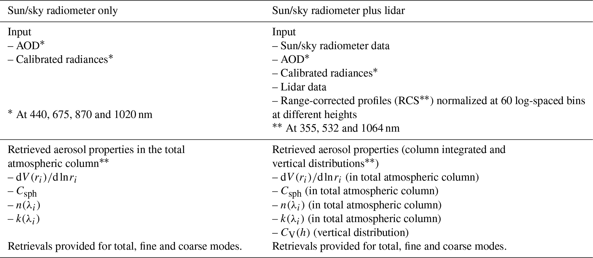
^* Azimuth angles, for sky radiances in the almucantar geometry, relative to the Sun (in ^∘): 3.0, 3.5, 4.0, 5.0, 6.0, 7.0, 8.0, 10.0, 12.0, 14.0, 16.0, 18.0, 20.0, 25.0, 30.0, 35.0, 40.0, 45.0, 50.0, 60.0, 70.0, 80.0, 90.0, 100.0, 110.0, 120.0, 140.0, 160.0 and 180.
${}^{**}$ Number of retrieved parameters is different for the different situations, and it is specifically described for each case in the text.

The detailed aerosol properties in the total atmospheric column provided by the AERONET inversion of sun/sky-scanning radiometers has been widely recognized as being rather unique, reliable data. For example, AERONET retrievals provided the first reliable data about aerosol spectral absorption and other detailed aerosol optical characteristics (e.g. see Dubovik et al., 2002b; Giles et al., 2012, and others). These detailed data are of vital importance for evaluating the impact of aerosol on such important aspects as a climate change and diverse pollution effects and can be reliable as they are estimated nearly uniquely from remote sensing observations (Kaufman et al., 2002). Therefore, this retrieved aerosol information has been proven to be very useful for the assessment of climate change dynamics in the Intergovernmental Panel on Climate Change (IPCC) reports (Boucher et al., 2013; IPCC, 2021) and other high-profile analyses.

As mentioned in earlier sections, the evaluations of the accuracy of retrieved aerosol parameters mainly relied on extensive sensitivity studies by Dubovik et al. (2000). The results were used for providing quality assurance criteria and expected accuracy estimation (see Dubovik et al., 2002b; Holben et al., 2006). Sinyuk et al. (2020) recently presented the approach to estimate retrieval uncertainties used in AERONET version 3 data. The approach estimates the error using the variability in retrieved parameters generated by 27 perturbations in both input measurements and auxiliary input parameters. In comparison with these previous efforts, this study evaluates the dynamic error estimates generated by the GRASP approach for each retrieval based on the measurement error propagation and bias estimations. This study estimates the complete covariance matrices of retrieval errors. In addition, the analysis of retrieval errors and their correlations conducted here also aims at demonstrating the value of the obtained estimates for understanding the retrieval error tendencies and optimizing the retrieval approaches.

3.1.2 Aerosol retrieval from a combination of sun/sky radiometers and lidar data

The inversion of co-located observations by sun/sky radiometers and lidar is another popular retrieval approach in the aerosol community. Indeed, radiometer direct sun and multiangular polarimetric observations of diffuse Sun radiation transmitted through the atmosphere have a significant sensitivity to the atmospheric aerosol amount, its particles size, shape and morphology; however, they have practically no sensitivity to the vertical variability in aerosols. The lidar observations, on the other hand, provide the information about the vertical distribution of aerosol, while their sensitivity to other aerosol properties is more limited compared to radiometer observations. Therefore, the information from co-located photometric measurements and lidar systems is complementary and always desirable for the enhanced characterization of aerosol properties. This complementarity is well recognized by the research community, and a large number of joint observational sites with both radiometer and lidar observations have been established in last decade. In these regards, the European ACTRIS (Aerosols, Clouds and Trace gases Research Infrastructure Network) infrastructure (https://www.actris.eu, last access: 12 August 2022) is one of the good examples of networks emphasizing the acquisition of diverse complementary observations at each site. All ACTRIS observational supersites possess both sun/sky radiometric and complex multiwavelength lidar systems.

GRASP retrieval has been successfully adapted by Lopatin et al. (2013) for processing such combined observations in an algorithm initially known as Generalized Aerosol Retrieval from Radiometer and Lidar Combined data (GARRLiC). This algorithm has been used in numerous studies (e.g. Granados-Muñoz et al., 2014; Granados-Muñoz et al., 2016; Tsekeri et al., 2017; Benavent-Oltra et al., 2017, 2019, 2021, and others) and was also adapted for the operational processing of lidar/radiometer observations in the frame of ACTRIS infrastructure. Later, the capabilities of GARRLiC/GRASP were significantly extended by Lopatin et al. (2021) for processing diverse, vertically resolved observations alone in a diverse combination with radiometric observations.

In these studies, we consider the aerosol retrieval from the base GARRLiC/GRASP input data set that includes AERONET sun/sky-scanning observations in the solar almucantar at four wavelengths and the lidar backscattering attenuation profile at three wavelengths at 355, 532 and 1064 nm (see Table 1). Thus, for the synergy of sun/sky radiometers and lidar measurements, we considered the same sun/sky radiometer input data combined with the correlative range-corrected signal (RCS) values at 355, 532 and 1064 nm. The lidar signal provided in GRASP as input data is normalized at 60 log-spaced bins at different heights, as in Lopatin et al. (2013, 2021), giving minimum and maximum heights. It is because all lidars provide observations within a certain distance range, which varies from instrument to instrument, and it is limited by emitter/receiver field of view overlap in the lower part and by the signal-to-noise ratio in the upper part. The GRASP inversion of these data derives, in addition to columnar aerosol properties provided from radiometer only inversion, the vertical profile of aerosol concentration. Moreover, the aerosol can be considered to be an external mixture of two aerosol components (fine and coarse). In such a case, all retrieved parameters are provided for both aerosol modes, as shown in the Table 1, where the number of the retrieved parameters in this case is 174 (120 values of the aerosol vertical concentration for fine and coarse modes, 25 size bins, seven values of RRI and IRI at each wavelength and for each mode, fine and coarse, and the sphericity fraction).

3.2 Analysis of the structure of different error parameters

As was already mentioned, GRASP has a capability to provide the full covariance matrix of the retrieval errors, and this study aimed to evaluate and illustrate the efficiency of these estimated covariance matrices. At the same time, retrieval error evaluations in most of the practical applications rely on the consideration of mainly diagonal elements of the covariance matrices, while non-diagonal elements of covariance matrices are much less common. Indeed, in spite of the fact that non-diagonal elements of covariance matrices provide valuable and interesting information about retrieval error correlations, these non-diagonal elements are not often available in practice, and the analysis of error correlations requires more sophisticated considerations compared to straightforward analysis diagonal elements only, and therefore, it is less popular. Considering these aspects, in the present study, as a first step, we make a more detailed and extensive analysis of the error variances, and then, as a second step, we illustrate the usefulness of obtained non-diagonal elements.

The performance of the GRASP error variances estimated, provided by Eqs. (25)–(27), is studied using a series of numerical tests. Figure 1 illustrates the general scheme of the organization of these tests.

Figure 1 General scheme for the validation of the error estimates.

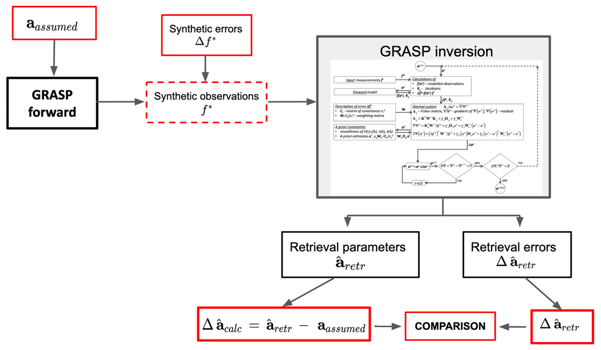
First, as showed in Fig. 1, the parameters a_assumed for the assumed detailed aerosol properties ($\mathrm{d}V\left(r_i\right)/\mathrm{d}\ln r_i$, n(λ_i), k(λ_i), C_sph and C_V(h) in the case of lidar) are used to obtain the synthetic observations using the GRASP forward model. These synthetic observations include the spectral AOD, sky radiances and range-corrected signals (RCSs) of lidar. These data are used then in the inversion tests where the aerosol parameters and their errors are estimated from these synthetic observations using the GRASP algorithm. In order to study the effects of the different uncertainties, both random and systematic errors are added to the synthetic measurements before the inversion, and then the retrieved parameters ${\widehat{\mathit{a}}}_{\mathrm{retr}}$ are compared with a_assumed (see Fig. 1). Therefore, from the retrieved parameters, the retrieval errors provided by the GRASP algorithm and actual retrieval errors can be compared. Thus, these actual errors are calculated comparing a_assumed and ${\widehat{\mathit{a}}}_{\mathrm{retr}}$ as follows:

$$\begin{array}{}\text{(34)}& \left\{\begin{array}{l}\mathrm{\Delta }{\widehat{\mathit{a}}}_{\mathrm{abs}}={\widehat{\mathit{a}}}_{\mathrm{retr}}-{\mathit{a}}_{\mathrm{assumed}}\\ \mathrm{\Delta }{\widehat{\mathit{a}}}_{\mathrm{rel}}={\displaystyle \frac{\mathrm{\Delta }{\widehat{\mathit{a}}}_{\mathrm{abs}}}{{\mathit{a}}_{\mathrm{assumed}}}}\cdot \mathrm{100}\mathit{\%},\end{array}\right.\end{array}$$

where ${\widehat{\mathit{a}}}_{\mathrm{retr}}$ is the retrieved parameter by the GRASP algorithm, and a_assumed is the parameter assumed in the input data for the generation of the synthetic observation. Equation (34) is used for each retrieved parameter, including the size distribution value at each size bin, the values of complex refractive index at each wavelength, the values of aerosol vertical profile at each altitude and the values of spherical particle fraction. We also implemented the evaluations of the errors for aerosol SSA and other parameters that are not part of the directly retrieved parameter while it is a function of the retrieved parameters, and it is estimated based on ${\widehat{\mathit{a}}}_{\mathrm{retr}}$. Thus, the retrieval error variances estimated by GRASP can be compared with the calculated actual retrieval errors. It should be noted here that we have always verified that the errors in the retrieval realized by GRASP from the error-free synthetic data (i.e. with no error specifically added) are negligibly small.

The GRASP-generated variances of the retrieval errors are evaluated in the presence of random errors and analysed using a series on the numerical tests conducted for a statistically representative set of random error realizations. These results are then summarized for the whole series of the tests by figures and tables. The tests with added systematic errors are discussed for most of the separate systematic error types, while some overall summaries are also provided.

As was mentioned before, in addition to the standard deviation, the non-diagonal elements of covariance matrices provide additional important insight about the retrieval quality. This additional information mainly relates to non-zero correlation coefficients. Therefore, in order to illustrate the correlation structure, in this work we also analysed the correlation matrix that contains the covariance matrix elements normalized by the respective variances, as shown by Eq. (33). Our studies are not attempting to evaluate correlation matrices provided by the GRASP algorithm, since this would require the efforts exceeding the scope of this paper. Instead, we try to provide several demonstrations of how the structure of the correlation matrix may help to understand several interesting observations in the existing retrieval experience.

3.3 Aerosols models and realizations used in the tests

The synthetic tests were performed for several preselected realizations of aerosol in the atmosphere. These realizations were selected based on extensive experience with aerosol retrieval from sun/sky radiometer data and their combination with co-located lidar data. It is expected that the selected aerosol realization scenarios are representative of the majority of distinct actual observations of atmospheric aerosols.

Two main observational scenarios are considered for different total aerosol optical depth at 440 nm.

• i.

  Single aerosol, such as biomass burning (BB), urban and dust for different aerosol loads τ(440)=0.3, 0.6 and 0.9.

• ii.

  The mixture of dust with BB and with urban (BB–Dust and Urban–Dust) is given. For each mixture, we have selected nine different scenarios that correspond to three different aerosol loads, τ(440)=0.2, 0.5 and 1.0, where the different cases of the partition between the fine and coarse mode were as follows: ${\mathit{\tau }}_{\mathrm{f}}/{\mathit{\tau }}_{\mathrm{c}}=\mathrm{4.0}$, ${\mathit{\tau }}_{\mathrm{f}}/{\mathit{\tau }}_{\mathrm{c}}=\mathrm{1}$, and ${\mathit{\tau }}_{\mathrm{f}}/{\mathit{\tau }}_{\mathrm{c}}=\mathrm{0.25}$.

The single-aerosol and aerosol mixture observational scenarios are used in the generation of synthetic tests with sun/sky-photometer-only observations. By considering both a single-aerosol and two aerosol types, in this work we evaluated how the accuracy of the retrieved data evolves once a larger number of parameters are derived from the same information content. In contrast, the retrieval based on the synergy between lidar and sun/sky photometers aimed for the retrieval of the properties of two fine- and coarse-mode aerosol components; therefore, the numerical tests for this type of the retrieval rely on the mixed aerosol observation scenario. At the same time, the error estimation is also checked in the case when the joint radiometer and lidar observations of single aerosol are analysed. The aerosol properties description used for the synthetic cases can be founded in Table 1 of Torres et al. (2017). They were modelled using the climatology of aerosol retrievals from AERONET observations described by Dubovik et al. (2002a). The dynamic climatological model from Mongu (Zambia) was used for BB aerosol, the model from the Goddard Space Flight Center (GSFC, Maryland, USA) for urban aerosol and the model from the Solar Village (Riyadh, Saudi Arabia) for dust aerosol. The real refractive index (RRI) and imaginary refractive index (IRI) for λ=355, 532 and 1064 nm (lidar measurements) were obtained by the extrapolation of the values from Dubovik et al. (2002a), as was suggested by Torres et al. (2017). All scenarios were simulated assuming a solar zenith angle (SZA) equal to 75^∘.

The retrieval settings were used similar to those that conventionally used in the retrieval of aerosol from AERONET sun/sky radiometer observations by Dubovik and King (2000) and from combined observations by sun/sky radiometer observations and lidar by Lopatin et al. (2013, 2021). Specifically, in the retrievals from sun/sky-radiometer-only observations, the size distribution (SD) was simulated using 22 logarithmically equidistant size bins between 0.05 and 15 µm. In the retrieval of the aerosol mixture from combined observations by sun/sky radiometers, the size distribution is modelled using 10 logarithmically equidistant bins between 0.05 and 0.58 µm for the fine mode and 15 logarithmically equidistant bins between 0.33 and 15 µm for the coarse mode. A similar approach was employed in the retrieval from sun/sky-radiometer-only observations when bicomponent aerosol model was retrieved.

As mentioned above, in the case of the joint processing of AERONET radiometer and lidar data, we considered the approach developed earlier by Lopatin et al. (2013). In frame of this approach, the aerosol is modelled as an external mixture of two components. These components are characterized by height-independent microphysical properties, including the size distribution (represented by several size bins) and spectrally dependent complex refractive index. Moreover, each component is described by the detailed vertical profile of the volume concentration. Therefore, the retrieval provides height-independent columnar properties of each component (size distribution and complex refractive index) and two profiles of fine- and coarse-mode volume concentrations. It is expected that this model is sufficient to adequately describe both radiometric and lidar observations.

4 Test results

Several tests were realized to evaluate the error estimates reliability and usefulness in the presence of both random and systematic uncertainties for aerosol retrievals from the observations of sun/sky radiometers alone and in combination with lidar. In this section, the results for the following two scenarios are presented: (i) a simpler case when only one type of aerosol is present and (ii) a more complex case in which two distinct types of aerosol are present at the same time. Moreover, we estimates the correlation matrices for both scenarios and illustrate their usefulness for understanding retrieval error tendencies, thus optimizing the retrieval approach.

4.1 Random error analysis

In a series of these tests of all inverted the synthetic measurements, we added random noise with a standard deviation of ε_Δτ(λ)=0.01 for AOD, ${\mathit{\epsilon }}_{\frac{\mathrm{\Delta }I}{I}}\left(\mathit{\lambda }\right)=\mathrm{5}$ % for radiances in order to model realistic uncertainties in AERONET observations (Holben et al., 1998; Eck et al., 1999; Dubovik et al., 2000; Sinyuk et al., 2020), ε₃₅₅=0.2, ε₅₃₂=0.15 and ε₁₀₆₄=0.1 for lidar attenuation measurements that vary with the altitude, as explained by Lopatin et al. (2013, 2021).

4.1.1 Retrieval of the single-aerosol component from radiometer measurements

This section describes the evaluation of the error estimates, assuming the presence of only one type of aerosol, i.e. BB, urban or dust. As mentioned before, the retrieval aerosol properties under the assumption of the presence of a single-aerosol type composed of homogeneous particles is a well-established approach for deriving detailed aerosol properties from ground-based observations by a sun/sky radiometer that is adapted by the operational AERONET retrievals by Dubovik and King (2000). The detailed error analysis of AERONET inversion aerosol product was provided by Dubovik et al. (2000), Torres et al. (2017) and by the recent study of Sinyuk et al. (2020) that described the uncertainty approach adapted in for AERONET version 3 retrieval products.

Figures 2–4 illustrate the error variances estimated by GRASP for all retrieved aerosol parameters in the selected synthetic tests for the observation of BB, urban and dust with different aerosol loads, i.e. τ(440)=0.3, 0.6 and 0.9. The displayed error bars for the standard deviation are calculated from the diagonal elements of the covariance matrix (Eq. 32). Some tendencies can be seen from these illustrations. For example, the errors in the SD in the extremes (for the largest and smallest particles) are the biggest. This is an expected tendency, since these particles typically have a lower contribution to the measured signal (radiances and aerosol optical depths) compared to the particles of intermediate radius.

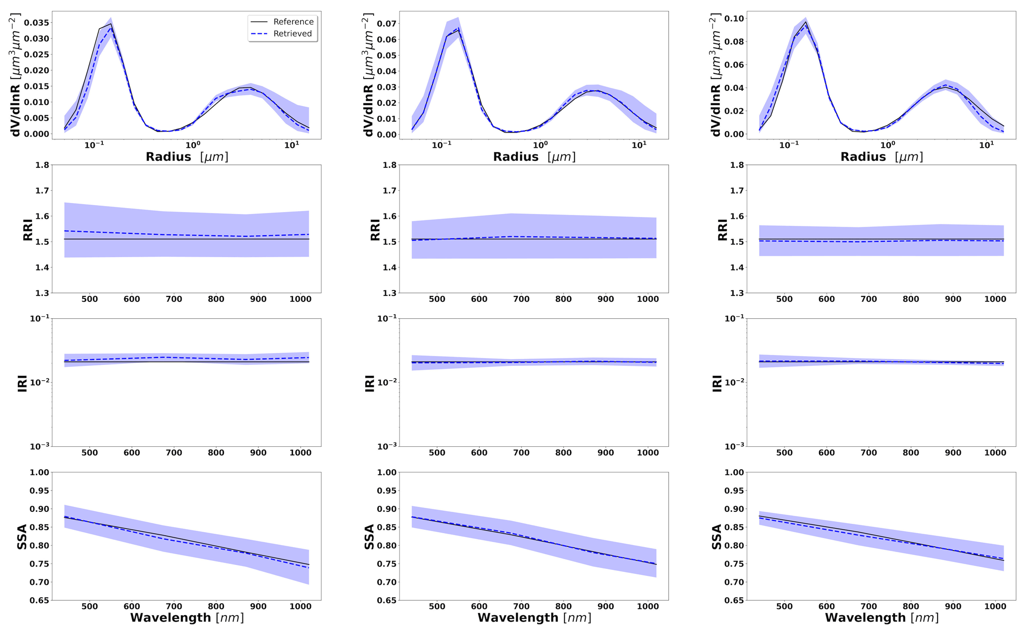
Figure 2 Aerosol properties retrieved from simulated sun photometer data, with random noise added for BB aerosols for τ(440)=0.3, 0.6 and 0.9 (left to right). The solid lines indicate the simulated properties (SD, RRI, IRI and SSA), and the dashed lines are the retrieved parameters. The shaded areas indicate error estimated by GRASP algorithm.

Figure 3 Aerosol properties retrieved from simulated sun photometer data, with random noise added for urban aerosol for τ(440)=0.3, 0.6 and 0.9 (left to right). The solid lines indicate the simulated properties (SD, RRI, IRI and SSA), and the dashed lines are the retrieved parameters. The shaded areas indicate error estimated by GRASP algorithm.

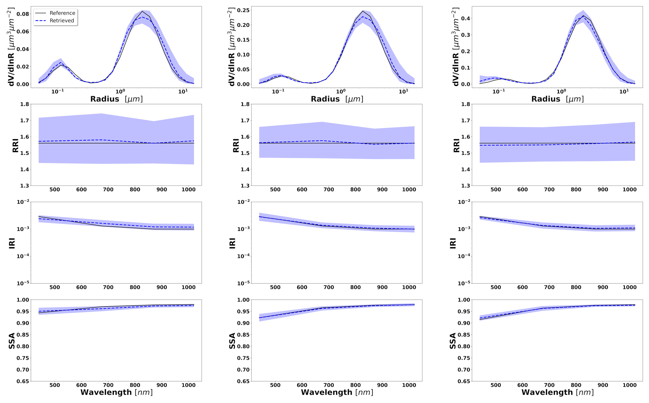
Figure 4 Aerosol properties retrieved from simulated sun photometer data, with random noise added for dust aerosol for τ(440)=0.3, 0.6 and 0.9 (left to right). The solid lines indicate the simulated properties (SD, RRI, IRI and SSA), and the dashed lines are the retrieved parameters. The shaded areas indicate error estimated by GRASP algorithm.

The retrievals improve and the errors decrease when the aerosol load increases, specially for IRI and SSA (absorption information). For BB and urban, the SSA error increases with the wavelength. On the other hand, SSA error decreases with the wavelength for dust. This is an expected behaviour, since the scattering efficiency is more pronounced at short wavelengths for small particles, while it is somewhat increasing with wavelength for large particles. Furthermore, as shown in Fig. 2a, the observed underestimation in the SD fine mode seems to be related to an overestimation in RRI.

To evaluate the error estimates in the presence of random noise, a set of the simulations for 300 different realizations of noise modelled using a random number generator has been analysed in this work. The results of such numerical tests conducted with a statistically representative set of random errors are summarized and illustrated, using box plots of the errors, as demonstrated in Fig. 5 for SSA(675) values. In the upper part of the figure, the box represents 50 % of the data, with the whiskers representing 5th and 95th percentiles of the data, the solid line in the box plot representing the median, and the points are the mean values.

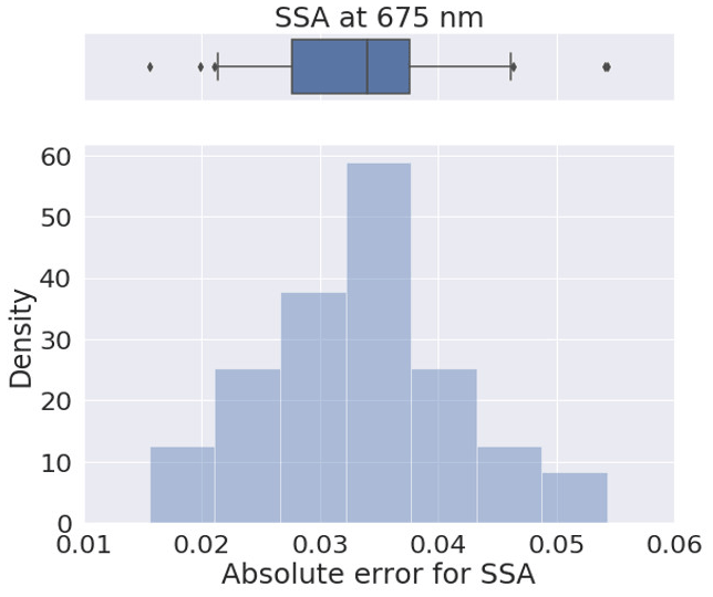
Figure 5 Comparison of the variance SSA(675) values estimated by the GRASP algorithm with actual errors obtained for extensive tests with randomly added modelled errors. In the upper panel, the box represents 50 % of the data, with the whiskers representing 5th and 95th percentiles of the data, and the solid line in the box plot representing the median value.

Figure 6 shows the distributions of the error estimates provided by GRASP (in red) and the calculated errors (in blue) for the cases when τ(440)=0.6 and the following convergence criteria are satisfied: Δτ≤0.01 % and $\mathrm{\Delta }I/I\le \mathrm{5}$ %. It can be seen that, overall, the error estimates provided by GRASP capture the actual error tendencies, with some overestimation of their values, quite well. Thus, the retrieved errors can be considered to be the upper estimates of actual errors. This observed general overestimation can be, at least partially, explained by the fact that the error estimates by Eqs. (23) and (24) rely on a linear approximation. In this respect, it is known from practice that the nonlinear effects often lead to some saturation, while that cannot be captured by linear estimates. Some interesting tendencies can be appreciated in the obtained illustrations. For example, errors in SSA increase with the wavelength for BB and urban and decrease for dust.

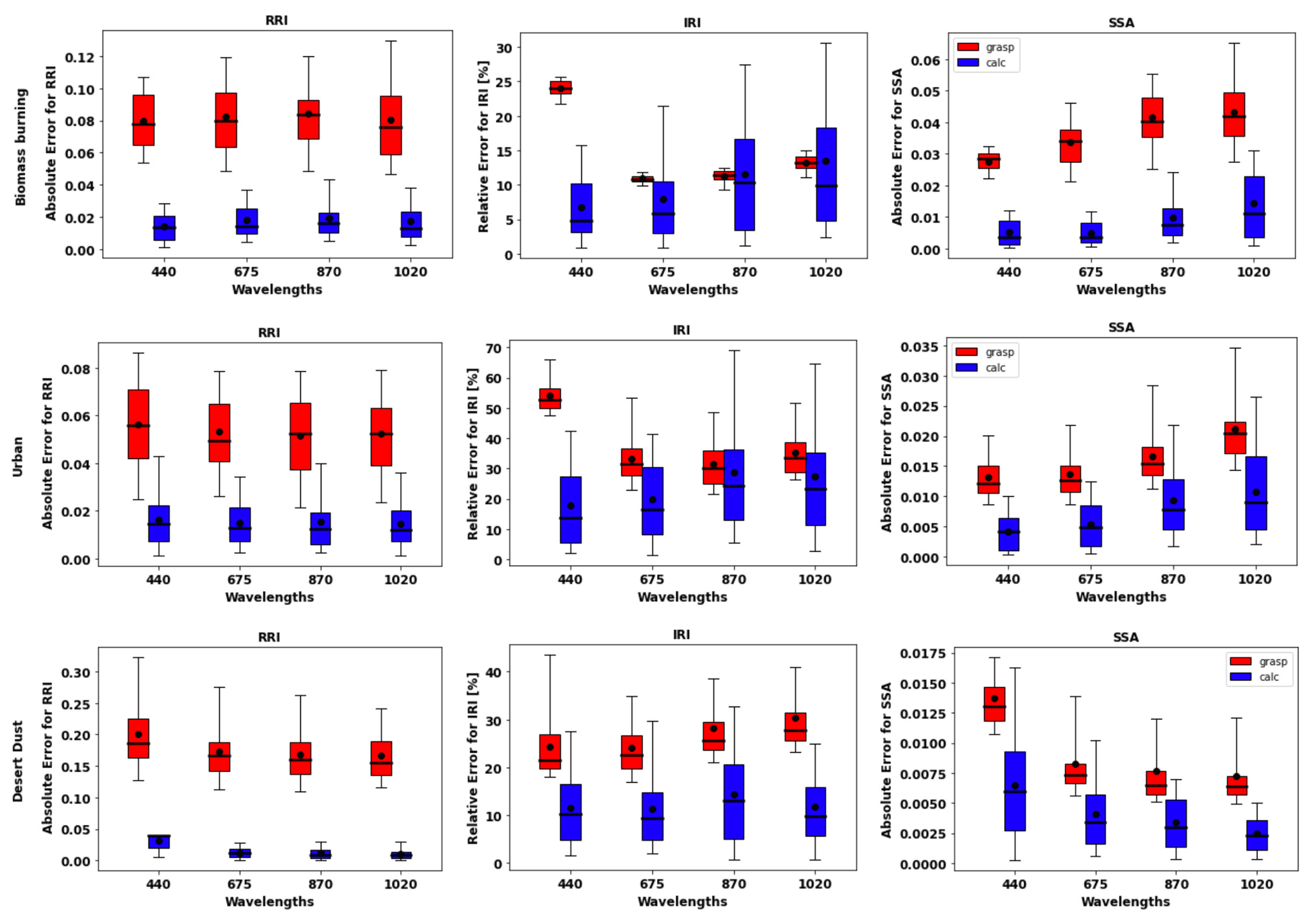
Figure 6 Comparison of estimated and actual error distributions for spectrally dependent aerosol parameters retrieved from sun/sky-photometer-simulated measurements (a case with τ(440)=0.6). The distributions were obtained using 300 realizations of added random errors. The median values of the errors are shown with a line in the box plot, along with the 25th–75th percentiles indicated by a box and the 5th–95th percentiles indicated using whiskers. The mean values are represented by the black dot. The red colour shows the error estimates provided by GRASP, and the blue shows the calculated actual errors (Eq. 34).

On the other hand, the RRI errors seem to be similar at the different wavelengths. This is likely related to the fact that, spectrally, RRI retrievals rely on rather strong smoothness constraints on spectral variability in RRI (e.g. Dubovik and King, 2000). In contrast to the RRI, a large variability in the calculated errors is observed in the distribution of the errors for the IRI. Indeed, in order to capture the possible real spectral variability in IRI as being that of dust (e.g. see Dubovik et al., 2002a), the IRI is retrieved under milder smoothness constraints on the spectral variability (see Dubovik and King, 2000). Some of the aforementioned and other tendencies in the retrieval errors will be further discussed and evaluated in Sect. 4.3.1, which deals with error correlation matrices.

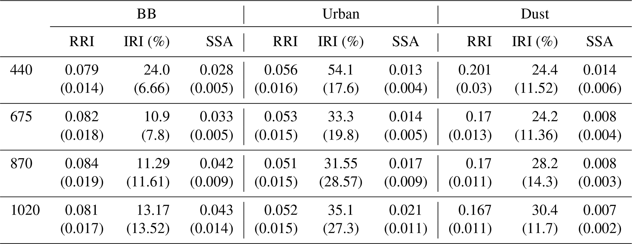
Table 2 summarizes the evaluation of the error estimates represented in the box plots. It provides the mean values for each parameter (RRI, IRI and SSA) at different wavelengths. These values correspond to the situation with a solar zenith angle equal to 75^∘. The obtained estimates compare reasonably with the corresponding values provided by in Table 4 in the paper by Dubovik et al. (2006). Specifically, the RRI error at 440 nm provided by GRASP for BB is 0.079 (0.04), where the values in parenthesis are from Dubovik et al. (2000), and for urban it is 0.056. The IRI error at 440 nm is 24 % (30 %) for BB, 54.1 % for urban and 24.4 % (50 %) for dust. The values of the SSA errors are 0.028 (0.03) for BB, 0.013 for urban and 0.014 (0.03) for dust. At the same time, the RRI error at 440 nm provided by GRASP for dust is 0.201 (0.04) and is quite different, although Dubovik et al. (2000) considered only spherical particles. Moreover, the error estimates for SSA are consistent with the U27 estimates provided by Sinyuk et al. (2020). For example, at 440 nm for AOD =0.6, the corresponding value for GSFC is 0.017, while GRASP provides values of 0.013; for Mongu, it is 0.023, while GRASP provides the error as 0.028.

Table 2 Errors provided by GRASP for the RRI, IRI and SSA are represented by the mean values of each box plot for their respective wavelength. Absolute errors are given for RRI and SSA and relative errors for IRI. Mean values of actual errors are provided in parenthesis.

4.1.2 Retrieval of mixed aerosol properties from measurements of a radiometer only

As already mentioned, most conventional aerosol retrievals from ground-based radiometer measurements (e.g. Dubovik and King, 2000; Nakajima et al., 2020) assume that aerosol is represented by homogeneous polydisperse particles with the size-independent refractive index. At the same time, this condition is not always correct in reality. Moreover, it is likely somewhat incorrect in the majority of the cases. Dubovik et al. (2000) showed that in some cases the retrieval assuming homogeneous particles would provide an effective index of refraction that allows the reproduction of the scattering properties of mixed aerosol rather adequately. Nonetheless, the assumption of homogeneous particles is often questioned and revisited (Xu et al., 2015); therefore, considerations of aerosol inhomogeneity are also included in the present study. In this regard, while the retrieval of the multicomponent aerosol is not a part of the standard AERONET inversion, the GRASP algorithm allows the retrieval of several aerosol components from diverse remote sensing observations, including the case of aerosol retrieval from radiometer measurements only.

At the same time, since the retrieval of multicomponent aerosol from radiometers only is not often used and not employed for operational retrievals, the tests in this section are limited to several illustrations only, and no statistical evaluation is performed. The illustrations are produced for the observations of a mixture of Urban–Dust and BB–Dust (see Sect. 3.3) for three cases of total τ(440)=0.2, 0.5 and 1.0. In particular, we illustrate the case for τ(440)=1.0, with τ_f=0.8 and τ_c=0.2, ${\mathit{\tau }}_{\mathrm{f}}={\mathit{\tau }}_{\mathrm{c}}=\mathrm{0.5}$ and τ_f=0.2, and τ_c=0.8, anticipating more potential for the adequate retrieval of multicomponent aerosol since the effect of AOD errors decreases for higher AOD. The analysis is focused on the possibilities of the differentiation between the properties of fine- and coarse-mode aerosol parameters such as complex refractive indices, size distributions, single scattering albedo.

Figures 7 and 8 illustrate the results of bicomponent retrievals and their error estimates from observations of the sun/sky radiometers of mixed aerosol. In the same figures, we also show a magnified plot for the effective RRI and IRI and the total SSA with their errors. Several retrieval tendencies are evident from the figures. For example, in the presence of one mode dominating in optical thickness, the retrievals and error estimates of the dominating component are more accurate. For example, in Fig. 7c for τ_f=0.2 and τ_c=0.8, the retrievals of the coarse-mode properties are more accurate. An opposite behaviour can be seen in Fig. 7a for τ_f=0.8 and τ_c=0.2, when the predominance is in the fine mode. The clear trend can be observed in spectral dynamic of the error values for SSA because the error increases with the wavelengths in the fine mode and decreases for the coarse mode.

Figure 7 Aerosol properties retrieved from simulated sun photometer data with random noise added for a mixture of Urban–Dust aerosols. The solid lines indicate the simulated properties (SD, RRI, IRI and SSA), and the dashed lines are the retrieved parameters. The shaded areas indicate the error estimated by the GRASP algorithm. The magnified plots represent the effective refractive index and total SSA.

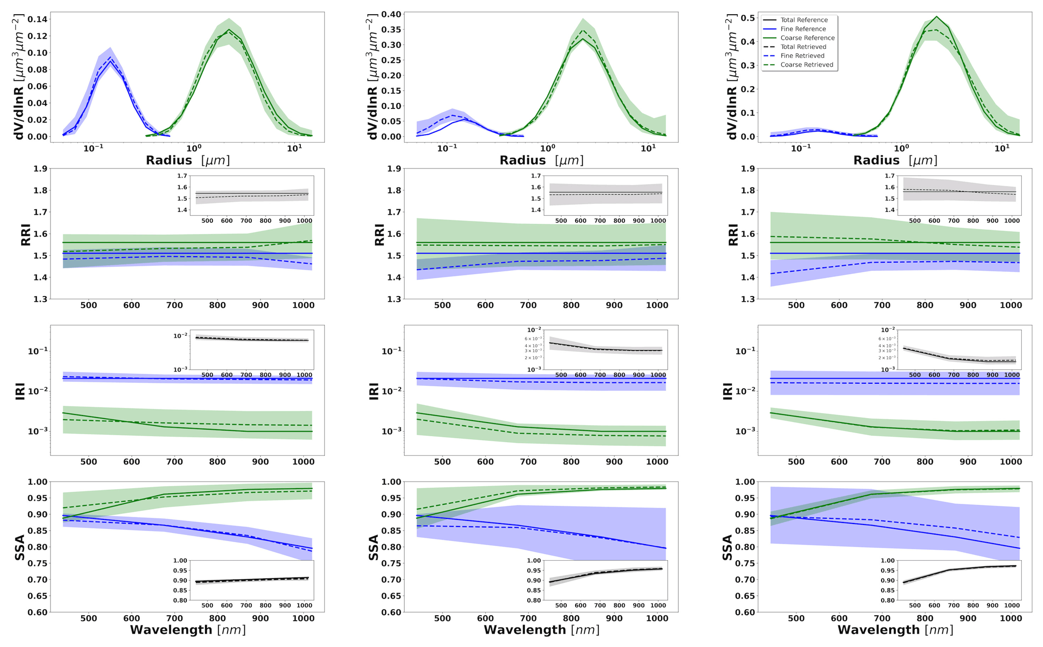
Figure 8 Aerosol properties retrieved from simulated sun photometer data with random noise added for a mixture of BB–Dust aerosols. The solid lines indicate the simulated properties (SD, RRI, IRI and SSA), and the dashed lines are the retrieved parameters. The shaded areas indicate the error estimated by the GRASP algorithm. The magnified plots represent the effective refractive index and total SSA.

The most obvious difficulties in the separation of modes are evident when the properties of each mode are not very different. For example, such a situation can be seen for IRI of the Urban–Dust mixture (Fig. 7) and for RRI of the BB–Dust mixture (Fig. 8). In such situations, the error variances of each parameter are large and likely correlated (more details are provided in the discussion of covariance matrices). However, it is very important to note that, while the discrimination of some parameters of each component separately is not evident, most of the total and effective properties (magnified plots) can be estimated rather accurately.

It should be noticed that the retrieval of the multicomponent aerosol from radiometric observations was added here to illustrate error transformation tendencies that are not evident. Indeed, the retrieval of multicomponent aerosol from the AERONET observation is very uncertain, as was shown, for example, by Dubovik et al. (2000). At the same time, some sensitivity to the presence of multicomponent aerosols exists, and the attempts of multicomponent retrievals distinguishing the two components are often encouraged by the aerosol community, especially for favourable situations when two aerosol components have comparable influence on AERONET measurements (the situation used in our tests). At the same time, such cases are very suitable for demonstrating that, if constraints are not sufficient, the errors can be unacceptably high and strongly correlated. At the same time, one can see that when some estimates are highly uncertain and strongly correlated, they still can be used for accurate estimation of their functions. For example, we showed that a property such as the total SSA of mixed aerosol can be rather accurately obtained from the retrieved SSA of fine and coarse modes. In the next section, we will also illustrate the improvements in multicomponent retrieval and error reduction when extra information is included, such as lidar measurements. In addition, the retrieval of the multicomponent aerosol used often becomes robust when co-located AERONET data are inverted together with data from co-located lidar (Lopatin et al., 2013, 2021).

4.1.3 Retrieval of mixed aerosol properties from the measurements of radiometers in combination with lidar

The GRASP aerosol retrieval from combined sun/sky radiometers and lidar observations were always designed for the retrieval of bicomponent aerosol (Lopatin et al., 2013), and the approach is employed for operational processing in the frame of ACTRIS activities. Therefore, the evaluation of the random error effect in the aerosol retrieval from radiometer and lidar observations of aerosol mixtures includes both the analysis of the selected illustrations and the statistically representative series of numerical tests with random errors. The considered synthetic data include synthetic observations produced for the same examples of aerosol mixtures (Urban–Dust and BB–Dust) as used in Sect. 4.1.2.

Figures 9 to 12 illustrate the retrievals and their error estimates obtained for aerosol properties of both fine- and coarse-mode aerosols. The good agreement of the actual retrieved parameters (solid lines) with the assumed values (dashed lines) can be seen for all cases. From a comparison of Figs. 7–8 with Figs. 9–10, it is easy to see that the retrieval error estimate is lower when lidar data are also used. The improvements (compared to the results from radiometer only retrievals) are especially evident in the separation of the retrieved aerosols properties, especially when the contribution of the aerosol load is lower (this will be shown in Sect. 4.2 when bias is also assumed). At the same time, the total properties are accurately estimated in both retrieval scenarios.

Figure 9 Aerosol properties retrieved from simulated sun photometer and lidar data with random noise added for a mixture of Urban–Dust aerosols. The solid lines indicate the simulated properties (SD, RRI, IRI and SSA), and the dashed lines are the retrieved parameters. The shaded areas indicate the error estimated by the GRASP algorithm. The magnified plots represent the effective refractive index and total SSA.

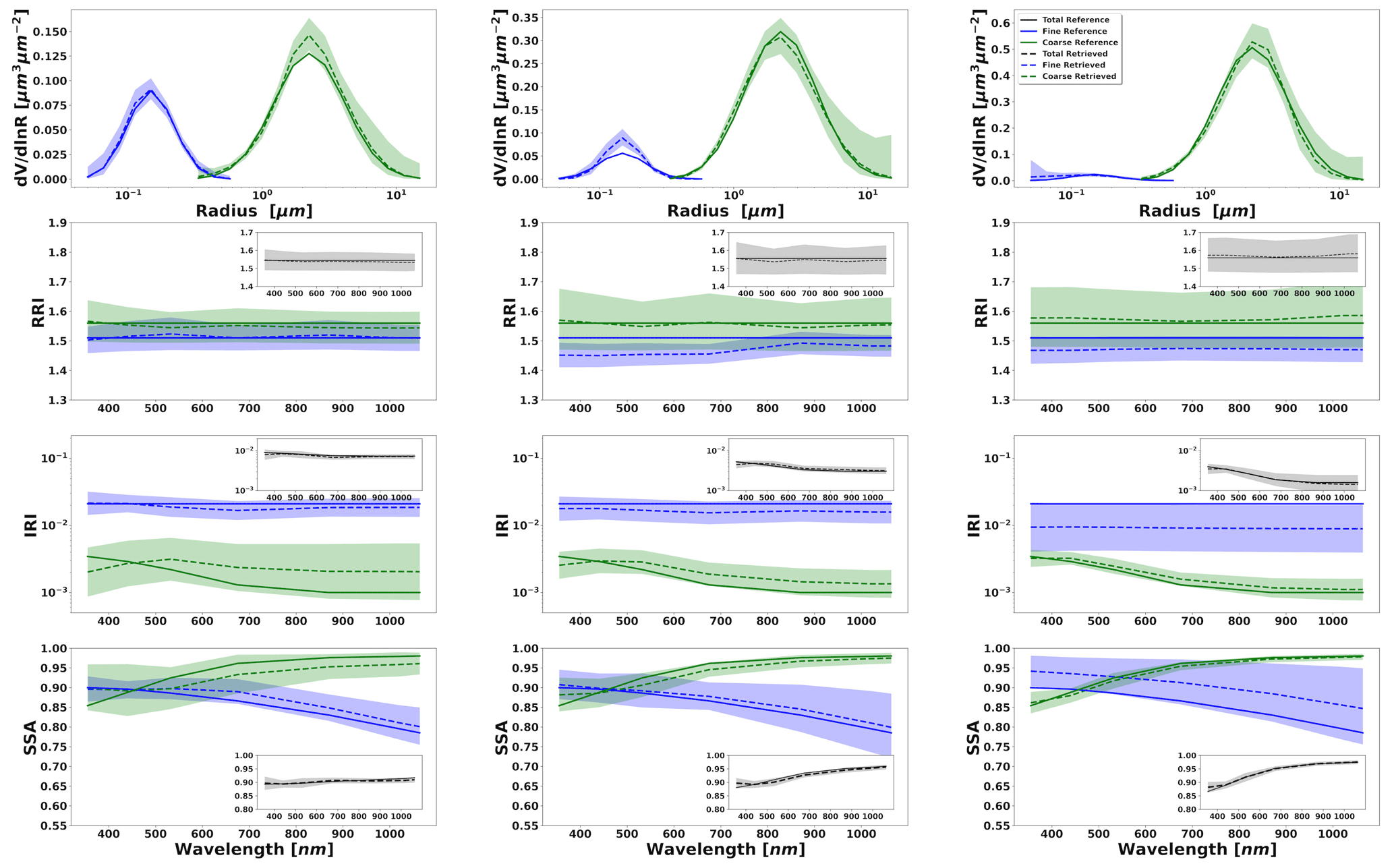
Figure 10 Aerosol properties retrieved from simulated sun photometer and lidar data with random noise added for a mixture of BB–Dust aerosols. The solid lines indicate the simulated properties (SD, RRI, IRI and SSA), and the dashed lines are the retrieved parameters. The shaded areas indicate the error estimated by the GRASP algorithm. The magnified plots represent the effective refractive index and total SSA.

Figure 11 shows the lidar ratio of the fine mode, coarse mode and total aerosol for the three aforementioned cases. In general, good agreements of retrieved and assumed values are obtained, especially for the total lidar ratio (LR). However, there are some discrepancies at short wavelengths for fine-mode lidar ratios.

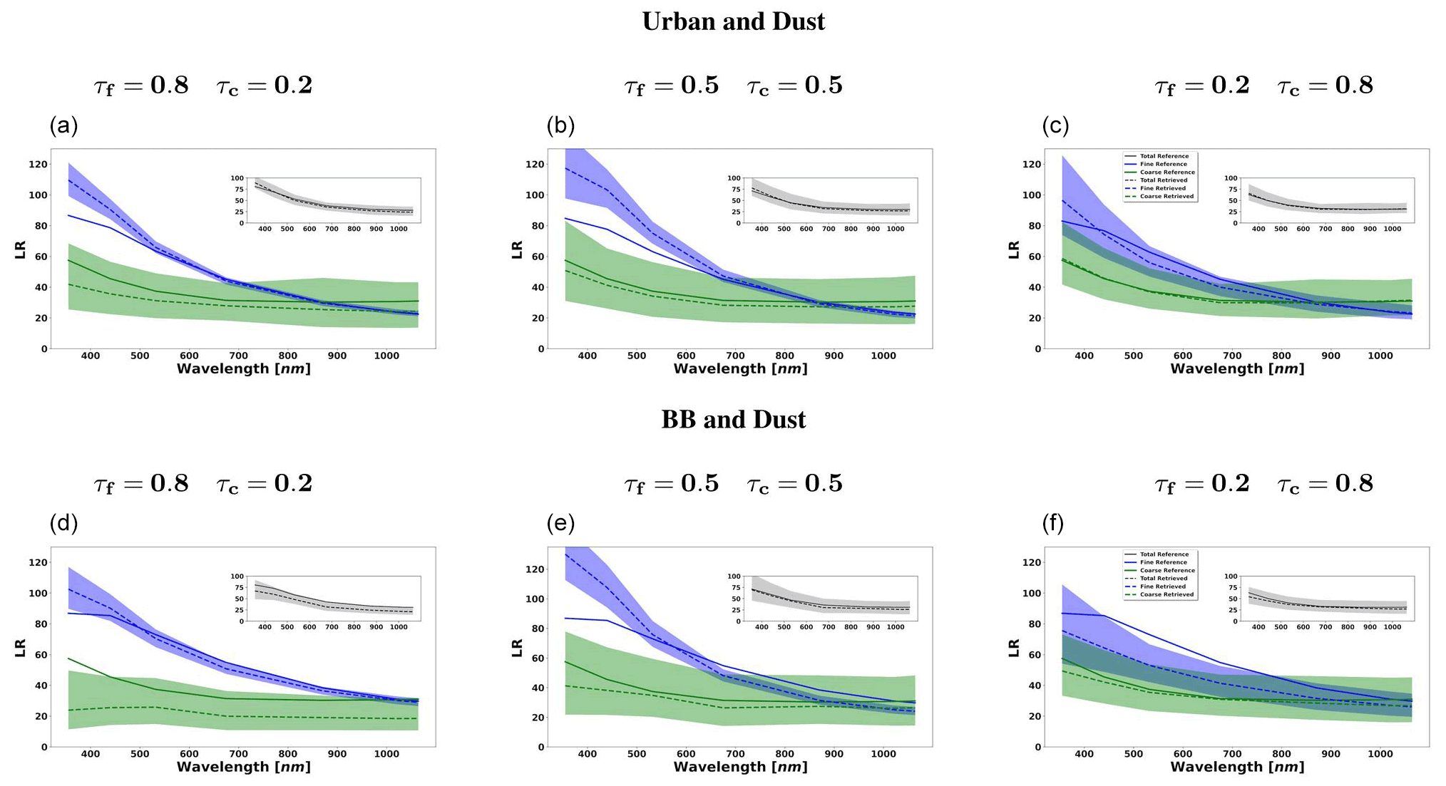
Figure 11 The aerosol lidar ratio (LR) retrieved from simulated sun photometer and lidar data with random noise added for a mixture Urban–Dust aerosols (above) and BB–Dust (below). The solid lines indicate the simulated properties (SD, RRI, IRI and SSA), and the dashed lines are the retrieved parameters. The shaded areas indicate the error estimated by the GRASP algorithm. The magnified plots represent the results for total LR retrievals.

Figure 12 illustrates the retrieval of aerosol vertical profile for each case. The agreement between the retrieved and assumed values of the vertical profiles is good, mainly for the coarse mode at the altitudes where it has maximum values and dominates. At the altitudes where there is a superposition of aerosol layers with a comparable presence of both aerosols, the retrieval struggles to discriminate the contribution of both modes, and a clear overestimation of the fine mode (and, consequently, an underestimation of the coarse mode) can be seen.

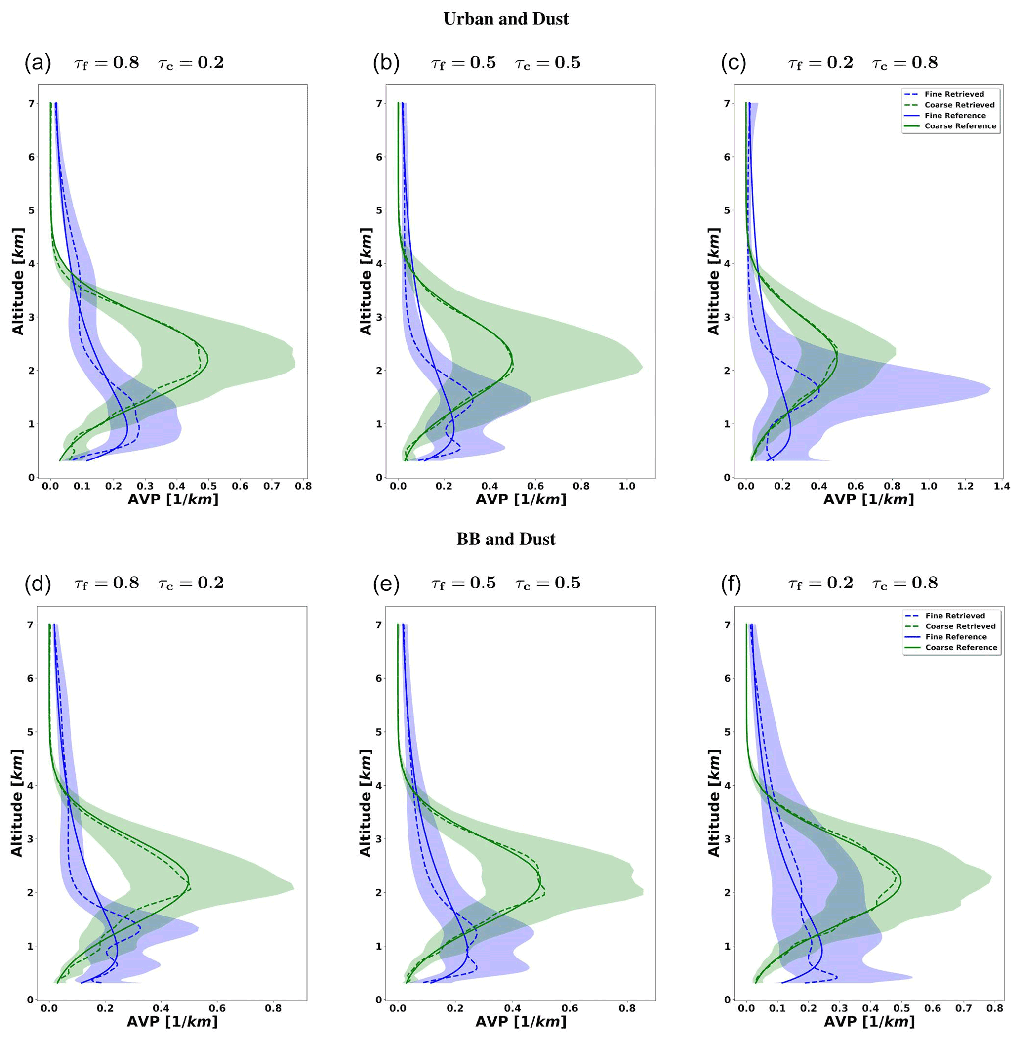
Figure 12 The aerosol vertical profiles (AVPs) retrieved from simulated sun photometer and lidar data with random noise added for a mixture of Urban–Dust aerosols (a, b, c) and BB–Dust (d, e, f). The solid lines indicate the simulated properties (AVP), and the dashed lines are the retrieved parameters. The shaded areas indicate the error estimated by the GRASP algorithm.

In order to evaluate the error estimates in the presence of random errors, a set of simulations, adding 300 realization of random noise values, is analysed. Figures 13 to 19 show the comparisons of all retrieved aerosol parameters separately for fine and coarse aerosol modes. In addition, the retrieval of total SSA and LR are shown. The case for total τ(440)=1.0 is shown more extensively, as in the previous section, due to the interest in the retrieval of the situation with higher aerosol loads. The main result that can be gained from illustrations is that the GRASP error estimates are typically higher than actual errors; this same result was obtained for the retrieval of only sun/sky radiometer data.

Figures 13 and 14 illustrate the comparisons of distributions of the GRASP error estimates and actual errors for RRI and IRI of fine and coarse aerosol modes for situations when mixtures of Urban–Dust and BB–Dust are observed. It can be seen that the accuracy of the refractive index retrievals for each mode depends strongly on the contribution of the mode to the signal, as was observed by Lopatin et al. (2013). For example, if we analyse the performance of the fine mode, the higher the contribution of the fine optical thickness, the better the accuracy in the retrievals of fine-mode aerosol parameters.

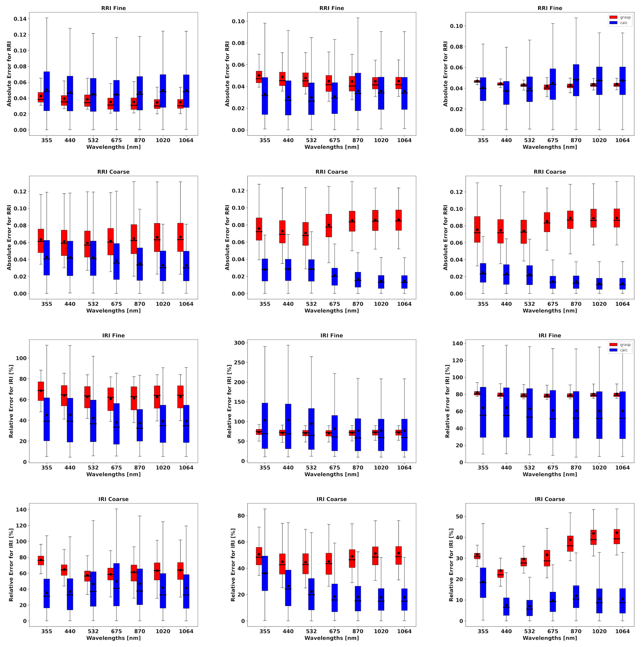
Figure 13 Comparison of estimated and actual error distributions for spectrally dependent aerosol parameters retrieved from measurements by simulated sun/sky photometer values and lidar for a mixture of Urban–Dust aerosol. The distributions were obtained using 300 realizations of added random errors. The median values of the errors are shown by a line in the box plot, along with the 25th–75th percentiles indicated by a box, and 5th–95th percentiles are indicated using whiskers. The mean values are represented by the black dot. The red colour shows the error estimates provided by GRASP, and the blue colour shows the calculated actual errors (Eq. 34).

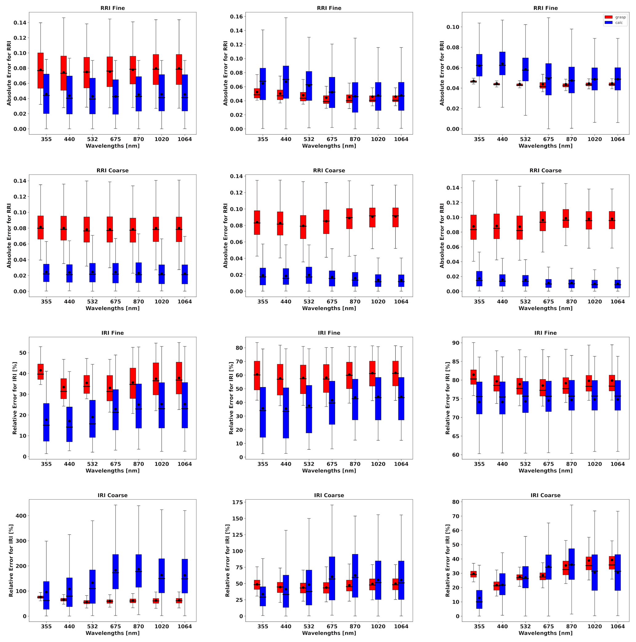
Figure 14 Comparison of estimated and actual error distributions for spectrally dependent aerosol parameters retrieved from measurements by simulated sun/sky photometer values and lidar for a mixture of BB–Dust aerosol. The distributions were obtained using 300 realizations of added random errors. The median values of the errors are shown by a line in the box plot, along with the 25th–75th percentiles indicated by a box, and 5th–95th percentiles are indicated using whiskers. The mean values are represented by the black dot. The red colour shows the error estimates provided by GRASP, and the blue colour shows the calculated actual errors (Eq. 34).

Figures 15 and 16 show the situation for the error distribution for SSA of fine mode, coarse mode and total. Similar to that observed in earlier tests for the retrieval of fine-mode parameters, the errors increase with the wavelength, while for the retrieval of the coarse-mode parameters, the errors decrease with the wavelengths. Also, the results show that the errors in the total SSA are rather small, even if the SSA of fine and coarse modes are quite high.

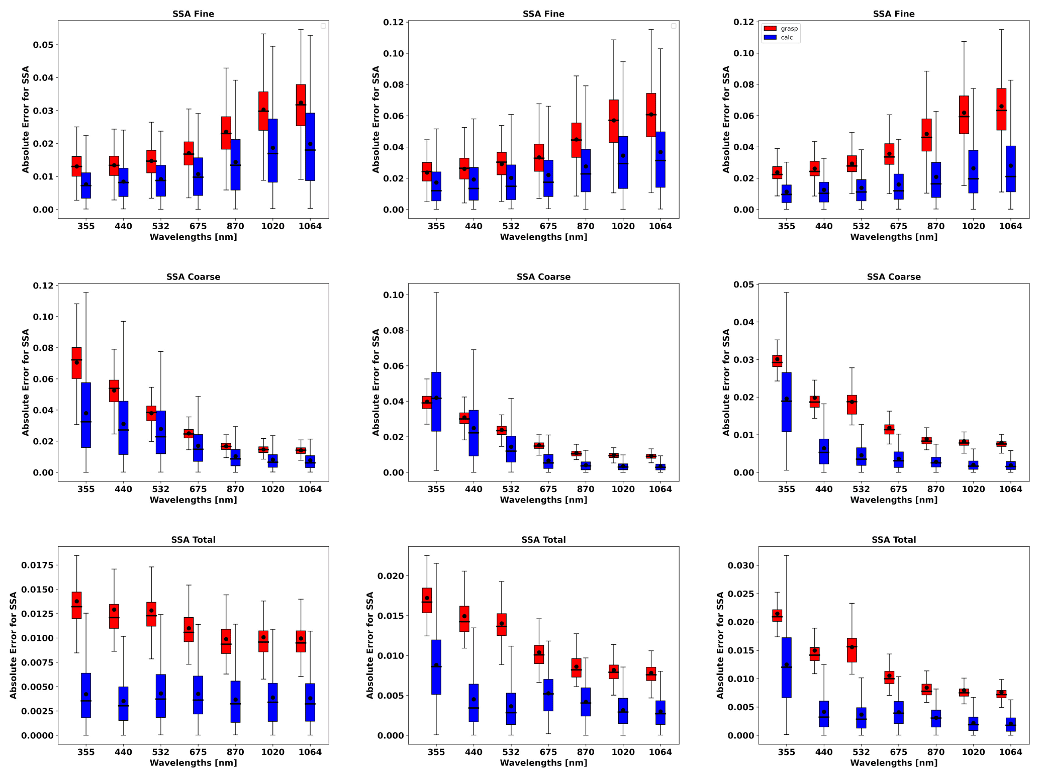
Figure 15 Comparison of estimated and actual error distributions for spectrally dependent aerosol parameters retrieved from measurements by simulated sun/sky photometer values and lidar for a mixture of Urban–Dust aerosol. The distributions were obtained using 300 realizations of added random errors. The median values of the errors are shown by a line in the box plot, along with the 25th–75th percentiles indicated by a box, and 5th–95th percentiles are indicated using whiskers. The mean values are represented by the black dot. The red colour shows the error estimates provided by GRASP, and the blue colour shows the calculated actual errors (Eq. 34).

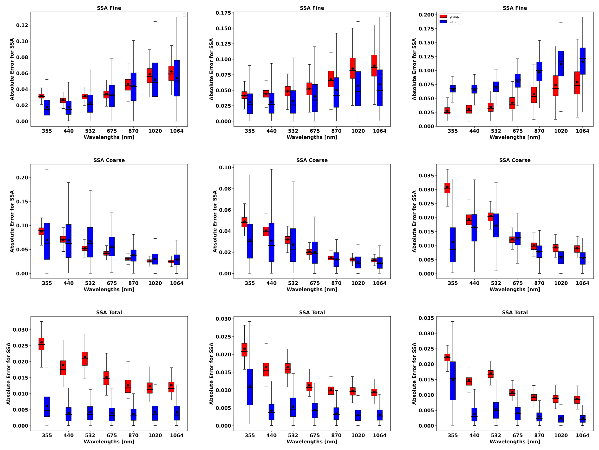
Figure 16 Comparison of estimated and actual error distributions for spectrally dependent aerosol parameters retrieved from measurements by simulated sun/sky photometer values and lidar for a mixture of BB–Dust aerosols. The distributions were obtained using 300 realizations of added random errors. The median values of the errors are shown by a line in the box plot, along with the 25th–75th percentiles indicated by a box, and 5th–95th percentiles are indicated using whiskers. The mean values are represented by the black dot. The red colour shows the error estimates provided by GRASP, and the blue colour shows the calculated actual errors (Eq. 34).

The error evaluation for LR is represented in Figs. 17 and 18. In most of the cases, we see good agreements between the error estimations and actual error. The only exception is the errors in the LR of the fine mode at short wavelengths, where the actual errors are higher than the errors provided by GRASP. This tendency seems to be anticorrelated with the results found for the coarse-mode LR error estimates, where the GRASP error estimates are notably higher than the actual values.

Figure 17 Comparison of estimated and actual error distributions for spectrally dependent aerosol parameters retrieved from measurements by simulated sun/sky photometer values and lidar for a mixture of Urban–Dust aerosols. The distributions were obtained using 300 realizations of added random errors. The median values of the errors are shown by a line in the box plot, along with the 25th–75th percentiles indicated by a box, and 5th–95th percentiles are indicated using whiskers. The mean values are represented by the black dot. The red colour shows the error estimates provided by GRASP, and the blue colour shows the calculated actual errors (Eq. 34).

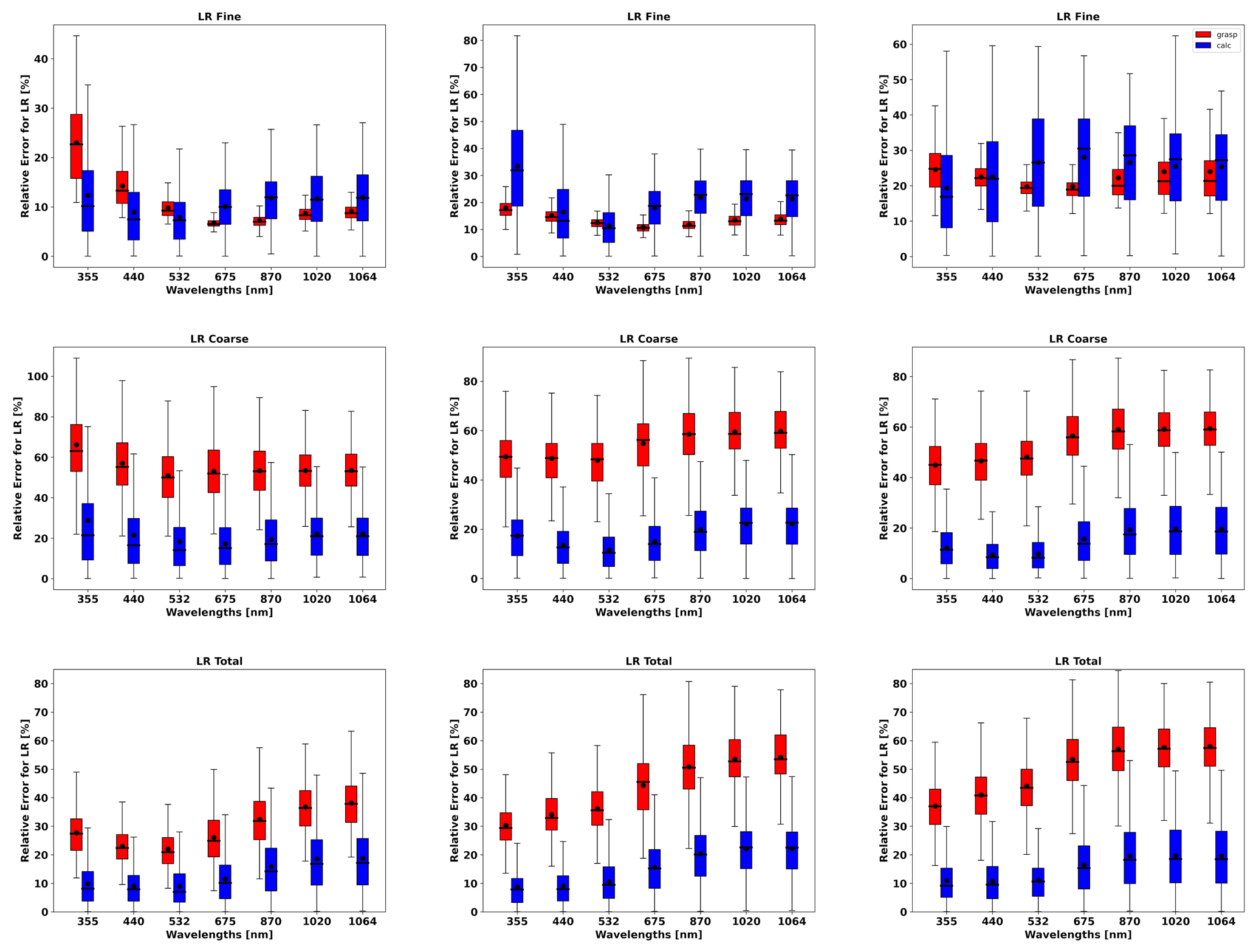
Figure 18 Comparison of estimated and actual error distributions for spectrally dependent aerosol parameters retrieved from measurements by simulated sun/sky photometer values and lidar for a mixture of BB–Dust aerosols. The distributions were obtained using 300 realizations of added random errors. The median values of the errors are shown by a line in the box plot, along with the 25th–75th percentiles indicated by a box, and 5th–95th percentiles are indicated using whiskers. The mean values are represented by the black dot. The red colour shows the error estimates provided by GRASP, and the blue colour shows the calculated actual errors (Eq. 34).

The results illustrated by the figures are summarized in Tables 3 to 5. These tables show the mean values of the GRASP error estimates for the cases when the total τ(440)=1.0 and ${\mathit{\tau }}_{\mathrm{f}}={\mathit{\tau }}_{\mathrm{c}}=\mathrm{0.5}$, i.e. when there is no predominance of either one of the modes. The values are provided for the aerosol parameter considered at different wavelengths, both for the simulation of Urban–Dust and BB–Dust observations calculated for a case of the SZA =75^∘.

Table 3 The mean values of RRI, IRI, SSA and LR retrieval errors estimated by GRASP for the synthetic test for a mixture of the Urban–Dust aerosol mixture. The mean values represent the distributions obtained using 300 realizations of the added random errors for the situation with total τ(440)=1.0, with ${\mathit{\tau }}_{\mathrm{f}}={\mathit{\tau }}_{\mathrm{c}}=\mathrm{0.5}$ and SZA =75^∘. The absolute errors are provided for RRI and SSA and relative errors for IRI and LR. Mean values for the actual errors are provided in parentheses.

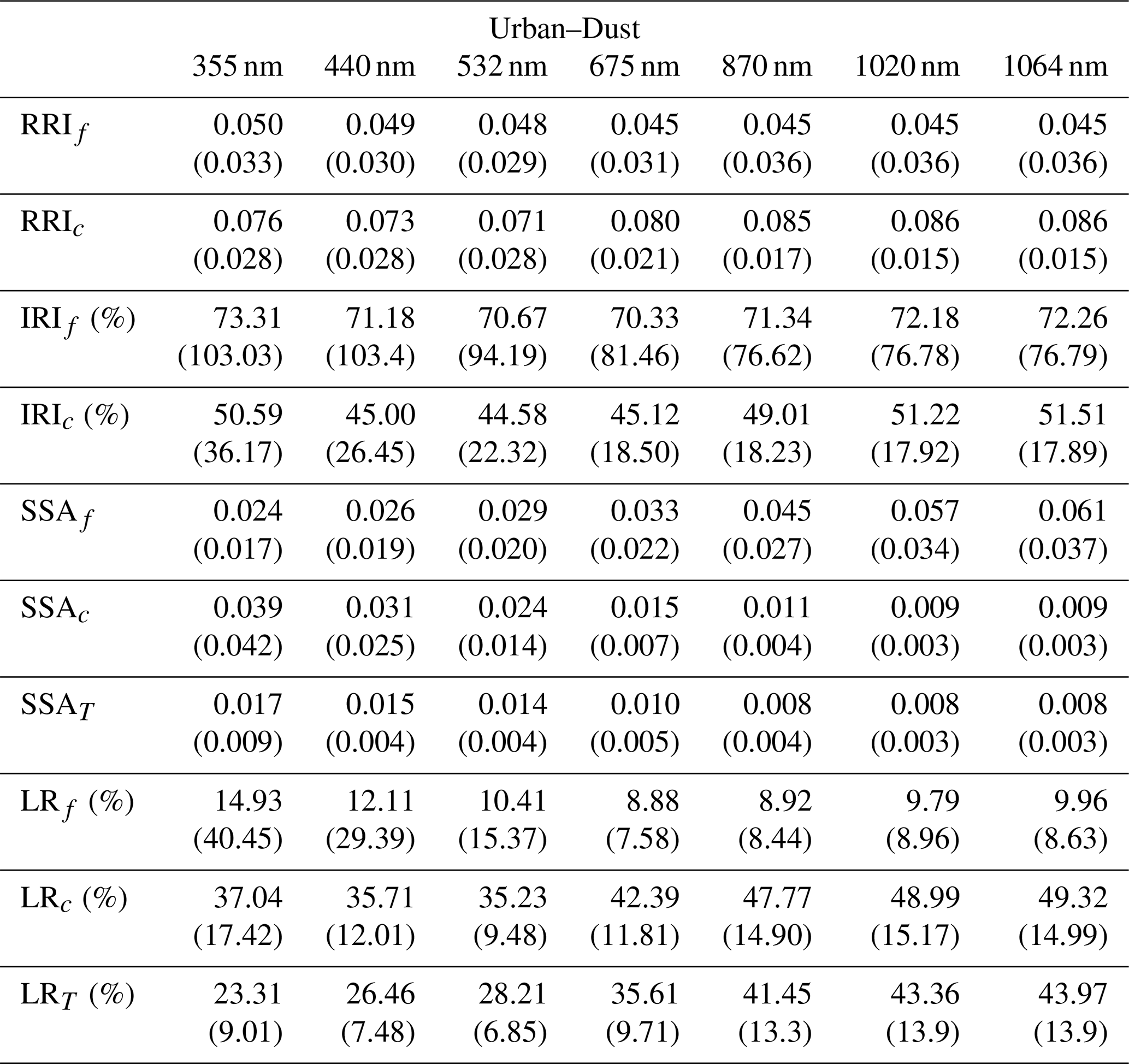
Table 4 The mean values of RRI, IRI, SSA and LR retrieval errors estimated by GRASP for the synthetic test for a mixture of the BB–Dust aerosol mixture. The mean values represent the distributions obtained using 300 realizations of the added random errors for the situation with total τ(440)=1.0, with ${\mathit{\tau }}_{\mathrm{f}}={\mathit{\tau }}_{\mathrm{c}}=\mathrm{0.5}$ and SZA =75^∘. The absolute errors are provided for RRI and SSA and relative errors for IRI and LR. Mean values for the actual errors are provided in parentheses.

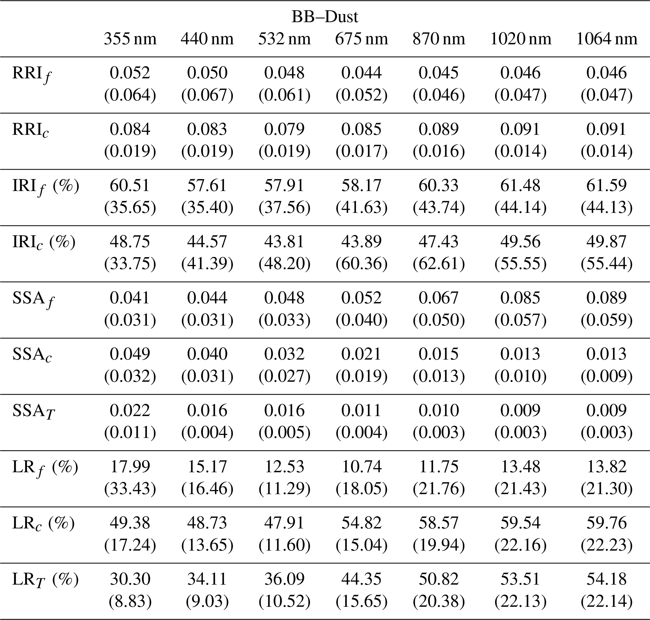
Table 5 The mean values of aerosol vertical profile (AVP) retrieval errors estimated by GRASP for the synthetic test for a mixture of the Urban–Dust aerosol mixture. The mean values represent the distributions obtained using 300 realizations of the added random errors for the situation with total τ(440)=1.0, with ${\mathit{\tau }}_{\mathrm{f}}={\mathit{\tau }}_{\mathrm{c}}=\mathrm{0.5}$ and SZA =75^∘. The shown relative errors for AVP (1 km) are represented by the mean values for three layers. Mean values for the actual errors are provided in parentheses.

For retrieval errors in fine mode in the case of urban aerosol parameters, the mean values for RRI are around 0.05, and the values do not present much variability with the wavelength. For the retrieval of IRI, the mean values of the GRASP retrieval errors are at the level of around 73 %, showing a pronounced underestimation with respect to the actual error at short wavelengths. With respect to SSA errors provided by GRASP, a clear tendency is observed because the error increases with the wavelengths from 0.024 to 0.061. Finally, the mean values of LR errors provided by GRASP decrease with the wavelength between 15 % and 10 %, with notable underestimations with respect to the actual errors at short wavelengths. In the case of the retrieval of fine-mode BB parameters, the mean values for RRI errors provided by GRASP are around 0.05. Some underestimations with respect to the actual errors are observed at short wavelengths. The mean values for IRI errors are around 60 %, and the errors for SSA show a clear tendency to increase with the wavelengths between 0.04 to 0.09. Mean values of LR errors provided by GRASP decrease with the wavelength between 18 % and 14 %.

The mean values of the error estimates provided by GRASP for dust present a good agreement in the case of both mixtures. In general, the mean values for RRI error estimates vary between 0.07 and 0.09, and they do not present much variability with the wavelength, while smaller values of errors are seen for the Urban–Dust mixture case. The mean values of IRI error estimates are around 50 %, while for the BB–Dust mixture, we observe some underestimations of the actual errors by GRASP calculations. The errors in SSA show a clear tendency that decreases with the wavelengths between 0.04 and 0.009. The mean values for the LR retrievals increase with the wavelength from 37 % to 60 %, with bigger errors observed for the BB–Dust mixture.

Once again, it is important to note that the errors in the parameters characterizing the total aerosol are generally accurately estimated. For both cases of Urban–Dust and BB–Dust mixtures, the mean values of the total SSA error estimates vary between 0.02 and 0.009, and the mean values of the total LR error estimates range from 23 % to 55 %.

Figure 19 shows the relative errors in AVP retrievals for fine and coarse aerosol modes for the Urban–Dust and BB–Dust aerosols mixture. The errors estimated by GRASP are a bit higher that the errors obtained by the simulations of random errors; correspondingly, the GRASP errors can be safely used as the upper estimates of actual retrieval uncertainties. Table 5 summarizes the evaluation of the errors estimates for all the scenarios discussed above. The GRASP estimates of the retrieval errors for both mixtures are between 50 %–70 % for the fine mode and 50 %–57 % for the coarse mode.

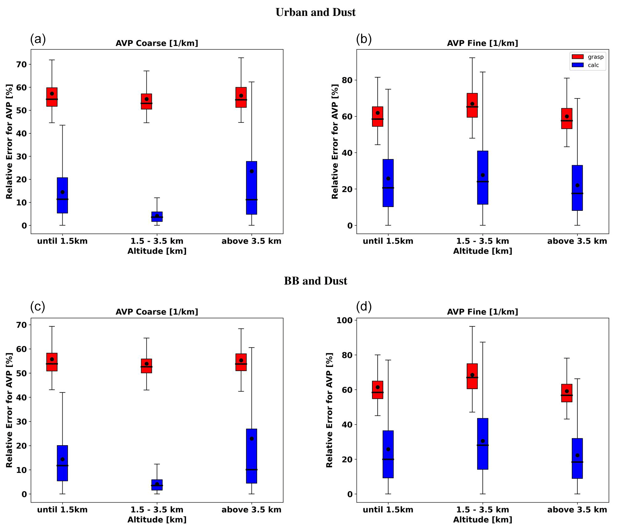
Figure 19 Comparison of estimated and actual error distributions for AVP retrieved from measurements by simulated sun/sky photometer values and lidar for a mixture of Urban–Dust aerosols (a, b) and BB–Dust (c, d). The distributions were obtained using 300 realizations of added random errors. The mean values are represented by the black dot, and the median values of the errors are shown by a line in the box plot, along with the 25th–75th percentiles indicate by a box, and 5th–95th percentiles are indicated using whiskers. The mean values are represented by the black dot. The red colour shows the error estimates provided by GRASP, and the blue colour shows the calculated actual errors (Eq. 34).

Finally, a lower sensitivity to the retrieval of fine-mode properties can be observed as a clear tendency in the evaluation of the retrieval errors for the cases when mixed aerosols are analysed. In particular, quite high errors were obtained for the complex refractive index. Then, these errors consequently propagate to the errors in other optical properties, such as the SSA of fine mode, as was found in the earlier study by Lopatin et al. (2013).

4.2 Analysis of the retrieval in presence of the systematic uncertainties

In Sect. 4.1, the evaluation and validation of the errors in the different aerosol properties, considering propagation of the random noise from measurements into retrieval, was presented. The analysis confirmed the rather satisfactory performance of the approach adapted in GRASP for the estimation of retrieval errors in the presence of random noise. This section discusses the approach for estimating the possible contributions of the systematic errors in the retrieval uncertainties. In principle, each retrieval methodology assumes that there are no systematic uncertainties in the measurements or in the forward model used. If any systematic bias is identified, it is corrected in the measurements or in their interpretation. However, in practice, the systematic uncertainties may remain unidentified and make a significant contribution to the retrieval uncertainties.

As mentioned above, in Eq. (24), the apparent misfit was used as an indicator of bias; however, in real situations, not all biases can be seen from the misfit. Thus, in this section, the results are presented considering a possible solution to this problem. Therefore, the contribution of potential bias is commonly included in the estimation of the retrieval errors (e.g.  see Dubovik et al., 2000; Sinyuk et al., 2020). Using similar logic, an extra term was added in the present methodology, Eq. (31), and then that accounts for the propagation of possible bias from the measurements. The propagation accounted for the linear approximation in similar manner to the systematic term in Eq. (28) that accounts for bias from misfit. Thus, this section analyses the potential effect of realistic biases and their overall importance for reliable estimations of the retrieval errors in practice.

The potential effect of the systematic errors is analysed in series of numerical tests with possible assumed systematic errors. Following previous studies by Dubovik et al. (2000); Torres et al. (2017); Sinyuk et al. (2020) in ground-based photometric and radiometric data, we consider two types of potential main biases in measured AOD and sky radiances. These biases could originate from the miscalibration of direct sun or diffuse sky sensors (Eck et al., 1999). The biases are assumed to be wavelength independent, and since spectral systematic deviations are easier to identify in a direct analysis of the observation, they are likely to be manifested in the misfit and may compensate for each other's influence on the retrievals. Specifically, two possible levels of biases, nominal and maximum, are considered to be as follows:

• i.

  In AOD, there is a nominal bias of ±0.01 and maximum bias of ±0.02.

• ii.

  In radiances, there is a nominal bias of ±3 % and maximum bias of ±5 %.

To evaluate the effects of biases, the above values were added to the synthetic direct measurements of AOD and sky radiance by an AERONET-like ground-based radiometer. These data were inverted by the GRASP code, and the retrieved values of aerosol parameters were compared to the values assumed in the synthetic simulation as a truth. In addition, the deviations in the retrieved values from the true ones are compared to the errors estimates generated by GRASP based on Eq. (31) using the known values of the added biases. In a similar manner, the influence of the potential systematic errors in aerosol retrieval from the combined observations of a ground-based radiometer and lidar was analysed. In these tests, the biases in the lidar attenuation measurements were assumed for each wavelength following the studies by Lopatin et al. (2013, 2021), with ${\mathit{\epsilon }}_{\mathrm{355}}=\pm \mathrm{0.2}$, ${\mathit{\epsilon }}_{\mathrm{532}}=\pm \mathrm{0.15}$ and ${\mathit{\epsilon }}_{\mathrm{1064}}=\pm \mathrm{0.1}$. It should be noted that the conducted synthetic tests not only allow the verification of the accuracy of the systematic error estimates by GRASP but also allow us to analyse the effects of biases on the retrievals for different retrieval scenarios in diverse situations.

4.2.1 Effects of measurement bias in the retrieval of single-aerosol components from radiometer measurements

In this section, the study is focused on the analysis of the effects of the biases and on estimating contribution of systematic errors in the retrievals of aerosol from ground-based observations by a radiometer. In a similar manner to the analysis of random errors, we first considered the observations dominated by two types of aerosols, i.e. BB and dust. The effect of measurement biases is expected to be manifested in the situations with low and moderate aerosol loading; therefore, the analysis is focused on the scenarios with AOD(440)=0.1, 0.3 and 0.6.

The following two situations were considered:

• i.

  when a single bias in AOD or radiances is present, and

• ii.

  when the biases can be present in both AOD and radiances simultaneously. In this case, the different combinations of positive and negative biases in AOD and radiances are considered.

The estimations of the errors introduced by the biases were calculated as follows:

$$\begin{array}{}\text{(35)}& {\mathit{\sigma }}_{\mathrm{bias}}^{\mathrm{2}}={\mathit{\sigma }}_{\mathrm{lm}}^{\mathrm{2}}+{\mathit{\sigma }}_{\mathrm{misfit}}^{\mathrm{2}}+{\displaystyle \frac{\mathrm{1}}{N}}\sum _{k=\mathrm{1}}^N{\mathit{\sigma }}_k^{\mathrm{2}},\end{array}$$

where ${\mathit{\sigma }}_{\mathrm{lm}}^{\mathrm{2}}$ corresponds to contributions from systematic errors introduced by the Levenberg–Marquardt procedure, and ${\mathit{\sigma }}_{\mathrm{misfit}}^{\mathrm{2}}$ are the errors manifested by the misfit estimated by Eq. (28), and each ${\mathit{\sigma }}_k^{\mathrm{2}}$ is the contribution adding + bias and − bias in the measurements.

Figures 20 to 23 illustrate the results of the analysis for the different retrieved properties for the situation with a bias of ±0.01 and ±0.02 in AOD only. These results show the specific effects from AOD bias. The figures have two blocks; on the left are the retrievals with added positive bias in AOD, and on the right, retrievals with negative bias are illustrated. In both cases, the error bars represent the systematic component adding the positive or negative bias, respectively. In all the figures, the solid lines show the assumed value of the parameters in the simulation, the dotted lines show the retrieved values, and the magnitudes of the estimated bias are shown by the shaded areas. It should be noted that, for the case of BB with AOD(440)=0.1, the results with negative bias are not shown. This is because the AOD for BB decreases very strongly with the wavelength, and for the case of AOD(440)=0.1, the AOD at 1020 nm is ∼0.01.

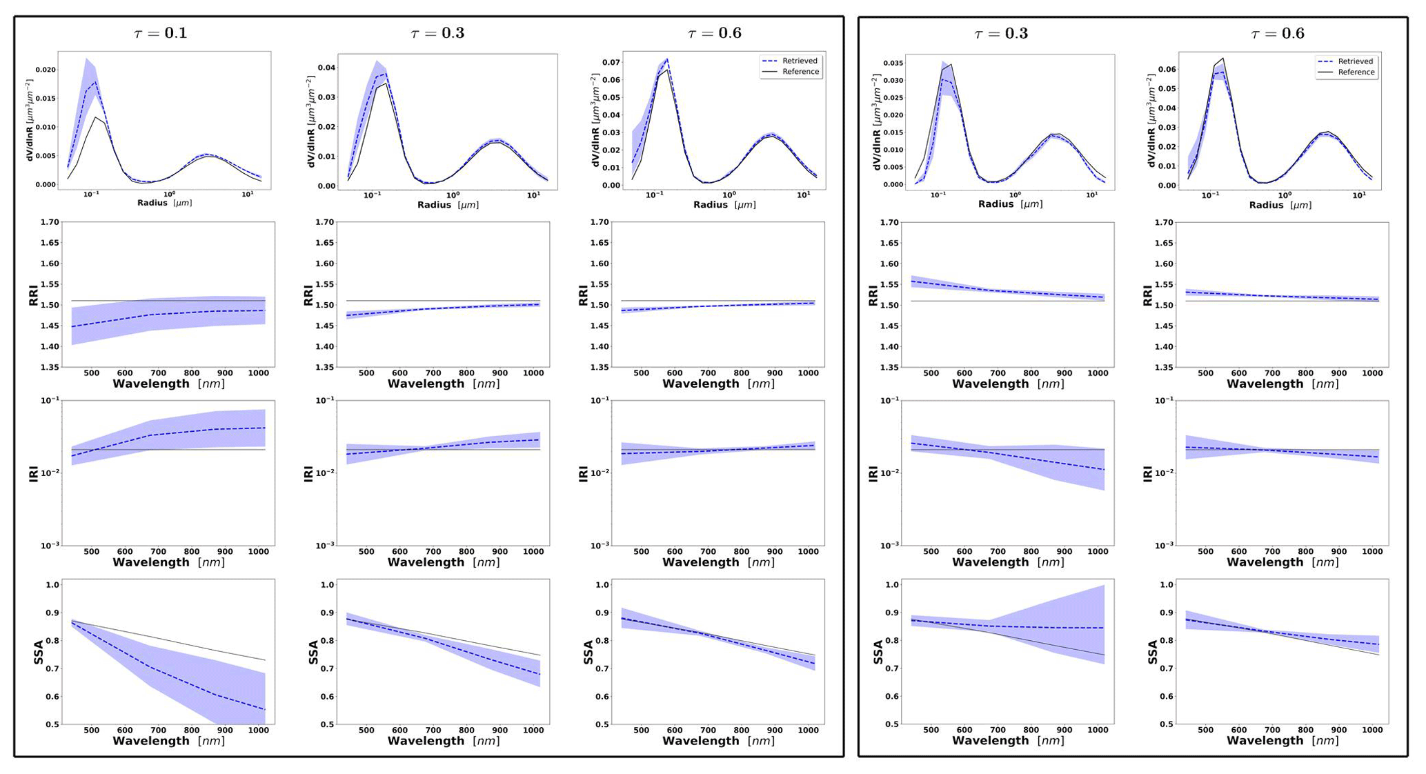
Figure 20 Aerosol properties retrieved from simulated sun/sky photometer data with assumed bias in AOD-simulated data for BB aerosol for τ(440)=0.1, 0.3 and 0.6 (left to right). Retrievals after adding the positive bias +0.01 are represented in the block on the left and negative bias −0.01 in the block on the right. The case for τ(440)=0.1 is not represented on the right side, since the AOD at 1020 nm is ∼0.01. The solid lines are the simulated properties (SD, RRI, IRI and SSA), and the dashed lines are the retrieved parameters. The shaded area indicates the systematic errors estimated by the GRASP algorithm.

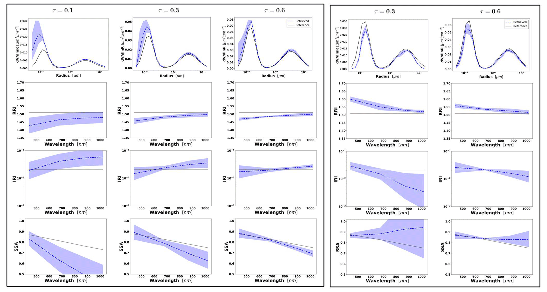
Figure 21 Aerosol properties retrieved from simulated sun/sky photometer data with assumed bias in AOD-simulated data for BB aerosol for τ(440)=0.1, 0.3 and 0.6 (left to right). Retrievals after adding the positive bias +0.02 are represented in the block on the left and negative bias −0.02 in the block on the right. The case for τ(440)=0.1 is not represented on the right side, since the AOD at 1020 nm is ∼0.01. The solid lines are the simulated properties (SD, RRI, IRI and SSA), and the dashed lines are the retrieved parameters. The shaded area indicates the systematic errors estimated by the GRASP algorithm.

The figures show different and clear tendencies, which are in agreement with general expectations, and with the tendencies already observed in previous studies by Dubovik et al. (2000) and Torres et al. (2014). For example, it can be seen that bias in AOD most strongly affects the estimate of the parameters characterizing the aerosol absorption, such as the imaginary part of the refractive index and single scattering absorption. This is an anticorrelation, where the positive bias results in the overestimation of absorption (higher RRI and lower SSA) and the negative in the underestimation of absorption (lower RRI and higher SSA), respectively. The result was expected, since radiance values in this first experience do not vary. Thus, if we keep the scattering component (which is derived from radiances) but we enlarge the extinction component (by enlarging the AOD) necessary, then the retrieval understands that the absorption should be larger (imaginary part of the refractive index). Conversely, if we reduce the value of extinction, then the retrieval would reduce the value of absorption. Also, the strongest effect is observed for optically thin situations when a small absolute error in the optical thickness becomes comparable with the magnitude of aerosol optical thickness. This is especially clear for BB observations, where AOD(1020) is always rather small as also discussed earlier by Dubovik et al. (2000). For the observations of dust aerosol, the effect of biases in AOD are significantly smaller than for BB. It can be explained since dust has a small value of the Ångström exponent and therefore larger values of AOD at longer wavelengths. For the retrieval of the size distribution, the bias in AOD has a rather minor effect, though we found a general overestimation for positive bias values and an underestimation for negative values.

Overall, the estimated systematic error agrees well with the actual manifestations of the bias in the retrieval. The quantitative estimations are also quite convincing and shown in Figs. 20 and 22 for biases of ±0.01. In some cases, some underestimations of the bias effects can be observed. For example, the largest differences are identified for the case of the higher value of bias (±0.02), as shown in Figs. 21 and 23, while a significant increase in the systematic component of the retrieved error is also well captured by the error estimates.

Figure 22 Aerosol properties retrieved from simulated sun/sky photometer data with assumed bias in AOD-simulated data for dust aerosol for τ(440)=0.1, 0.3 and 0.6 (left to right). Retrievals after adding the positive bias +0.01 are represented in the block on the left and negative bias −0.01 in the block on the right. The solid lines are the simulated properties (SD, RRI, IRI and SSA), and the dashed lines are the retrieved parameters. The shaded area indicates the systematic errors estimated by the GRASP algorithm.

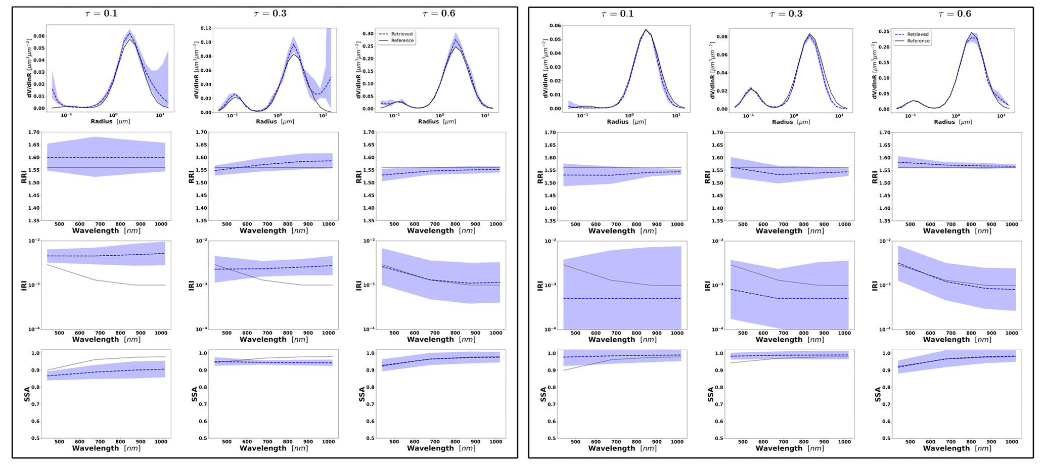
Figure 23 Aerosol properties retrieved from simulated sun/sky photometer data with assumed bias in AOD simulated data for dust aerosol for τ(440)=0.1, 0.3 and 0.6 (left to right). Retrievals after adding positive bias +0.02 are represented in the block on the left and negative bias −0.02 in the block on the right. The solid lines are the simulated properties (SD, RRI, IRI and SSA), and the dashed lines are the retrieved parameters. The shaded area indicates the systematic errors estimated by the GRASP algorithm.

It can be seen that, among all considered aerosol parameters, the main differences between the bias effects and the obtained error estimates are observed for the real part of the refractive index (RRI). In these cases, the bias is not fully covered by the systematic component of the retrieved error results. Similarly, an apparent underestimation of the RRI errors was also seen by Sinyuk et al. (2020), who attributed these underestimations to different factors such as, for example, the effect of not accounting for the pointing bias. In the present simulations, there is no pointing bias considered, and the discrepancy is likely coming from the fact that Eqs. (24) and (31) rely on the derivatives estimated in the vicinity of the solution and based on linear approximation. Indeed, the dependence of both AOD and radiances scattered by aerosol is very complex and nonlinear. Therefore, with both taking derivatives in the vicinity of obtained solution instead of the vicinity of the true values and the nonlinear character of AOD and radiances may explain the differences. At the same time, it is important to note that, as can be seen from the analysis of the random component of the RRI error (Sect. 4.1), the random error effect is likely to dominate over the effect of AOD bias, and therefore, the estimation of the total error (described below in this section) seems to allow us to make an objective and complete observation on this parameter.

Figures 24 to 27 show the effects of the biases in the radiances of the two magnitudes of ±3 % and ±5 % for the observations of BB and dust. In general, it can be seen from the results that, in both cases of BB and dust, the retrievals are less affected by bias in the radiances than by the biases in the AOD, even when the bias in the radiances is ±5 %. A similar tendency was also reported in the studies by Dubovik et al. (2000), Torres et al. (2014) and Sinyuk et al. (2020). At the same time, it should be noted that the present analysis is focused on the measurement configuration corresponding to solar almucantar when the SZA is 75^∘ (see Table 1) and when the measurements include are taken in a wide range of scattering angles. In this respect, Dubovik et al. (2000) showed that the effect of the sky radiance bias increases when the range of observed scattering angles is limited, i.e. in almucantar observation corresponding to a SZA of less than 60^∘. Moreover, according to recent tendencies in observational practices, the use of such measurements is limited, and most analyses are focused on observational scenarios with a sufficient range of observed scattering angles. For example, AERONET start to establish so-called hybrid observational scenario during high SZA times (Giles et al., 2019). With regard to the performance of the error estimation, the effect of the bias in the sky radiances seems to be well captured by the GRASP error estimates.

Figure 24 Aerosol properties retrieved from simulated sun/sky photometer data with assumed bias in AOD-simulated data for BB aerosol for τ(440)=0.1, 0.3 and 0.6 (left to right). Retrievals after adding the positive bias +0.03 are represented in the block on the left and negative bias −0.03 in the block on the right. The solid lines are the simulated properties (SD, RRI, IRI and SSA), and the dashed lines are the retrieved parameters. The shaded area indicates the systematic errors estimated by the GRASP algorithm.

Figure 25 Aerosol properties retrieved from simulated sun/sky photometer data with assumed bias in AOD-simulated data for BB aerosol for τ(440)=0.1, 0.3 and 0.6 (left to right). Retrievals after adding the positive bias +0.05 are represented in the block on the left and negative bias −0.05 in the block on the right. The solid lines are the simulated properties (SD, RRI, IRI and SSA), and the dashed lines are the retrieved parameters. The shaded area indicates the systematic errors estimated by the GRASP algorithm.

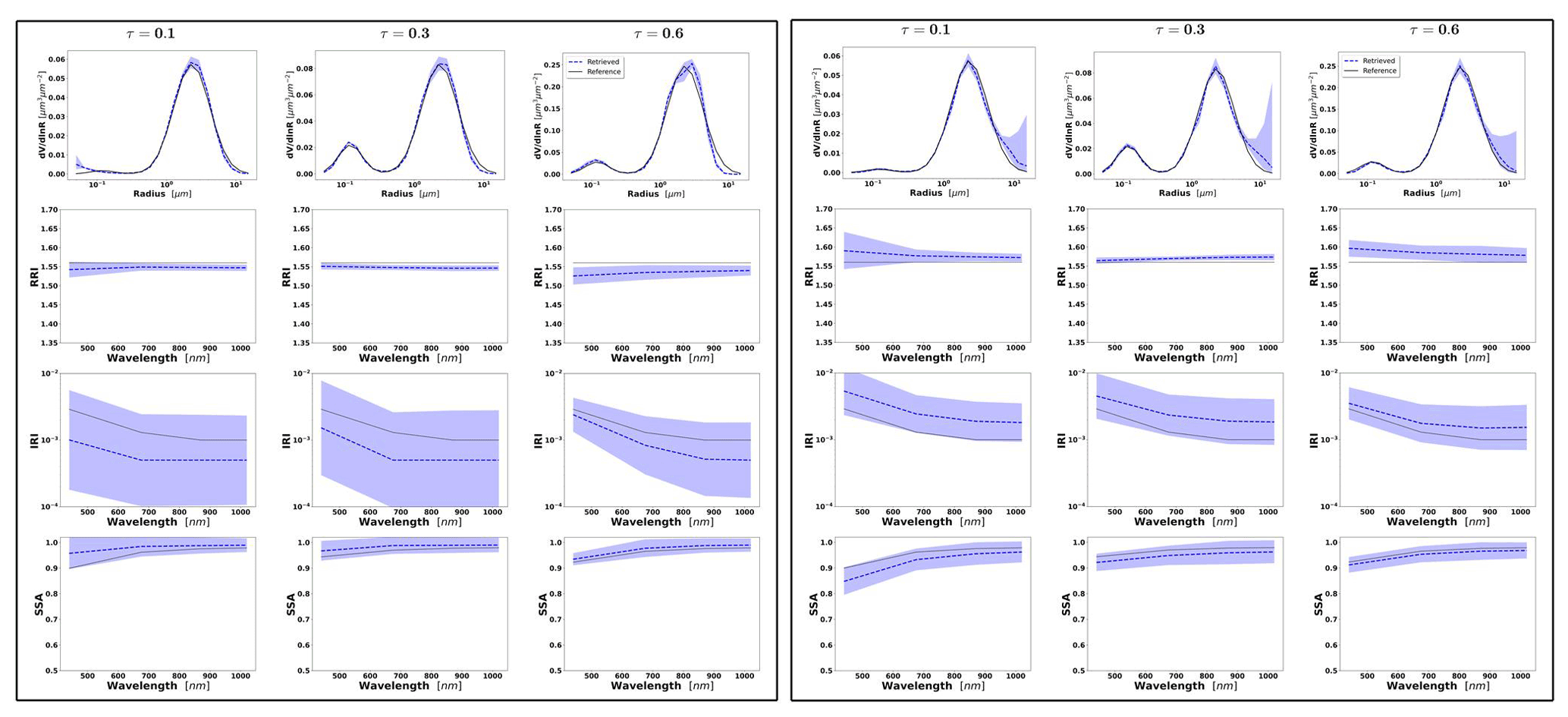
Figure 26 Aerosol properties retrieved from simulated sun/sky photometer data with assumed bias in AOD-simulated data for dust aerosol for τ(440)=0.1, 0.3 and 0.6 (left to right). Retrievals after adding the positive bias +0.03 are represented in the block on the left and negative bias −0.03 in the block on the right. The solid lines are the simulated properties (SD, RRI, IRI and SSA), and the dashed lines are the retrieved parameters. The shaded area indicates the systematic errors estimated by the GRASP algorithm.

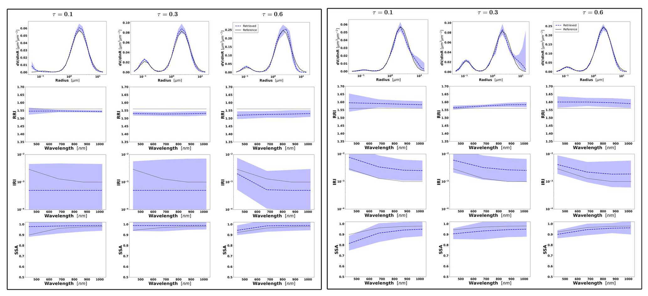
Figure 27 Aerosol properties retrieved from simulated sun/sky photometer data with assumed bias in AOD-simulated data for dust aerosol for τ(440)=0.1, 0.3 and 0.6 (left to right). Retrievals after adding the positive bias +0.05 are represented in the block on the left and negative bias −0.05 in the block on the right. The solid lines are the simulated properties (SD, RRI, IRI and SSA), and the dashed lines are the retrieved parameters. The shaded area indicates the systematic errors estimated by the GRASP algorithm.

It should be also noted that we observe an anticorrelation between the radiance bias and the retrieval of the imaginary part of the refractive index. This effect is opposite to the one observed in the case of AOD and with significantly smaller differences. Thus, when the biases are positive (+3 % and +5 %), there is a decrease in the imaginary part of the refractive index. The fact that the value of AOD remains the same and that there is an increase in the value of the scattering is interpreted by the code as a decrease in the aerosol absorption. Conversely, the negative bias in the radiances produces an increase in the imaginary part of the refractive index which can be explained by the same reason.

Figure 28 shows the results of the analysis of the situation when the systematic biases present in both AOD and radiances are simultaneously assumed. The results for BB are on the left and for dust on the right. The illustrations are shown for the specific situation with two positive biases, namely +0.01 in AOD and +5 % in radiances. It should be noted that the tests were produced for both situations with the biases of the same and opposite signs. This case with the biases of the same sign showed the most interesting results with the strongest manifestation of bias effects, and therefore, they are presented here. In the situation with biases of opposite signs, the effects on the retrievals are rather minor due to the internal compensations of the influences of the biases. Additionally, the misfit of the observations is more pronounced, which helps to identify the issues and account for the biases in the error estimates. Also, the analysis here is focused on the simultaneous biases of moderate values (±0.01 in AOD and ±5 % in radiances), since the appearance of simultaneous biases of the highest bias values (i.e. ±0.02 in the AOD and ±5 % in radiancies) lead to very strong effects in the retrievals. Those situations can be easily seen and screened out by quality filters (e.g. by the high value of the misfit). Also, it is quite unlikely to have such strong systematic errors in practical observations as those by AERONET.

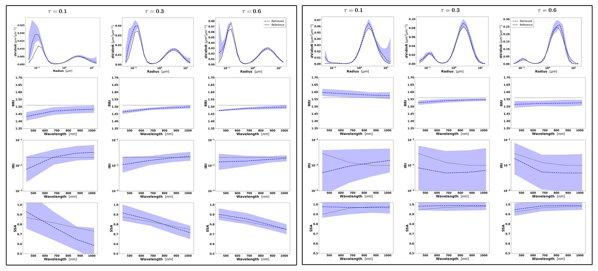
Figure 28 Aerosol properties retrieved from simulated sun/sky photometer data with assumed bias in AOD- and radiance-simulated data for BB (left) and dust (right) aerosol for τ(440)=0.1, 0.3 and 0.6 (left to right). Retrievals after adding positive bias +0.01 in AOD and +5 % in radiances are represented in both cases. The solid lines are the simulated properties (SD, RRI, IRI and SSA), and the dashed lines are the retrieved parameters. The shaded area indicates the systematic error estimated by the GRASP algorithm.

As can be seen from Fig. 28, the biggest differences and highest bias values in the retrieval are found for low AOD (0.1). As seen earlier for this situation, the errors for the RRI remain notably underestimated. As already mentioned, the situation is expected to be improved once the effects of both random and systematic errors are considered.

Figure 29 illustrates such a situation for the retrieval of BB and dust for the three different aerosol loads (0.1, 0.3 and 0.6) when the total error estimate includes both random and systematic components as follows:

$$\begin{array}{}\text{(36)}& {\mathit{\sigma }}_{\mathrm{tot}}=\sqrt{{\mathit{\sigma }}_{\mathrm{ran}}^{\mathrm{2}}+{\mathit{\sigma }}_{\mathrm{bias}}^{\mathrm{2}}},\end{array}$$

where ${\mathit{\sigma }}_{\mathrm{bias}}^{\mathrm{2}}$ is calculated as indicated in Eq. (35).

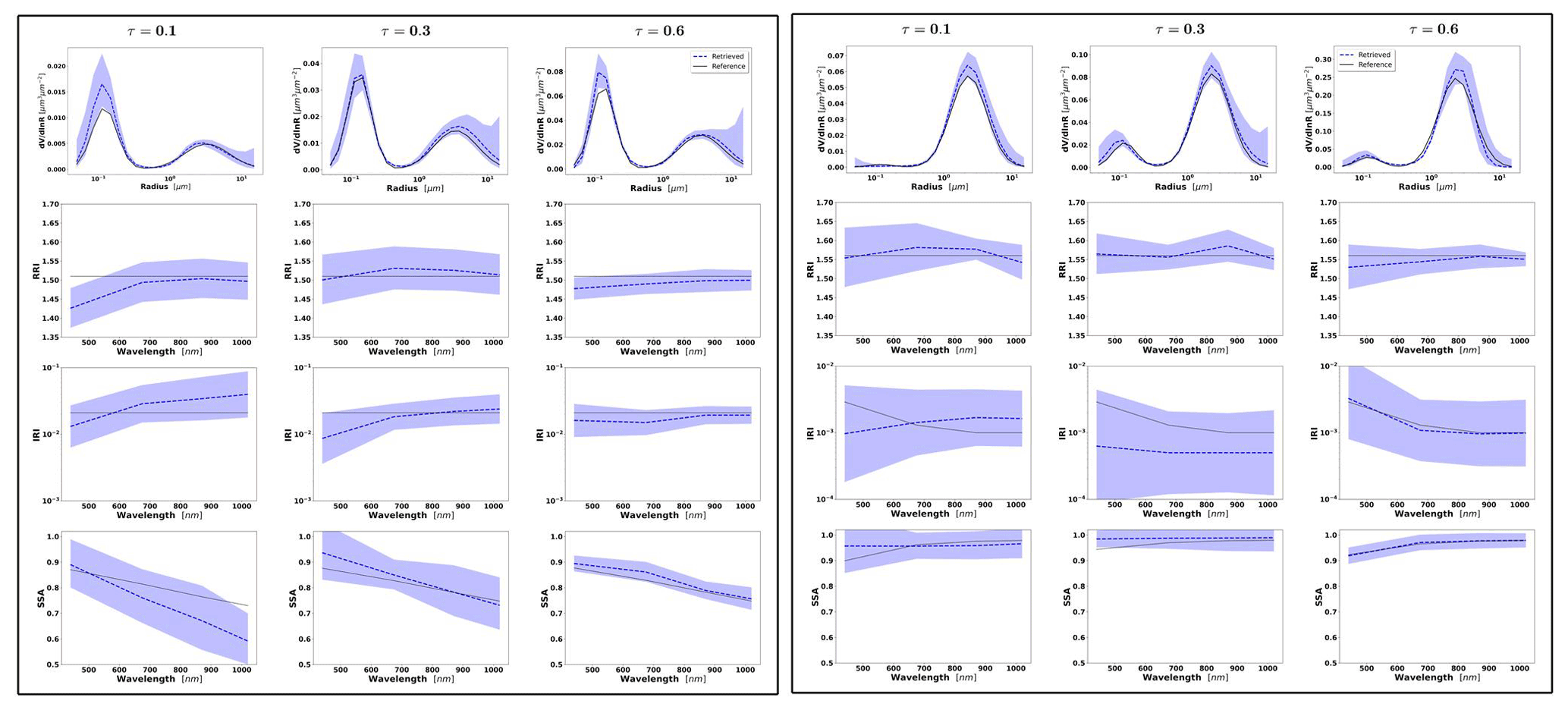
Figure 29 Aerosol properties retrieved from simulated sun/sky photometer data with assumed bias in AOD- and radiance-simulated data for BB (left) and dust (right) aerosol for τ(440)=0.1, 0.3 and 0.6 (left to right). Retrievals after adding positive bias +0.01 in AOD and +5 % in radiances are represented in both cases. The solid lines are the simulated properties (SD, RRI, IRI and SSA), and the dashed lines are the retrieved parameters. The shaded area indicates the systematic error estimated by the GRASP algorithm.

It can be seen that the total error estimates capture the deviations for all parameters in the presence of random and systematic noise. These results confirm that the estimations using Eq. (31), based on the additional assumptions of potential presence of bias in the measurements, improve the results of the error estimated compared to the approach discussed in Sect. 4.1, when the effects of biased were taken into account only based on the value of the observation misfit. The observed tendencies in the effects of biases on the retrieval are consistent with all the results previously described in earlier studies. The obtained results are expected to be representative of most practical situations, while some additional tests and analysis could certainly be useful. Therefore, in the examples presented below, and for the real cases analysed, the total error will be used as described in Eq. (36). This means that the representation of the error will take into account the contribution of the random and systematic component. This last component contains the contribution of Levenberg–Marquardt and the misfit and the measurements in which the contributions of ± bias added in the measurements are considered (Eq. 35). These values of the assumed biases in our applications are consistent with AERONET as mentioned previously, i.e. ±0.01 in AOD and ±5 % in radiances.

4.2.2 Effects of measurement bias in the retrieval of mixed aerosol properties from measurements of radiometers only

The present section tries to understand how the bias is affected when inhomogeneous aerosol are observed. The example is not commonly considered in practical application, e.g. in AERONET operational processing. At the same time, since GRASP can consider this type of bicomponent inversion that is fundamentally of high interest, we are analysing this situation in the presence of biases. In Sect. 4.2.1, we have shown different examples, considering the bias in each measurement separately, and we have also illustrated the complete example with presence of both random errors and bias in all the measurements. Here we directly illustrate the results, considering the presence of both random and bias in all the measurements, since this is complete situation that is closest to the most practical situation.

Different tests were performed for this study. In particular, we focus on the case of BB–Dust, since Sect. 4.2.1 has already demonstrated the bias affects when each type of aerosol is observed separately. The effects of each bias separately were analysed, while the corresponding illustrations are not shown since the results presented similar tendencies to those previously discussed and are observed for each type of aerosol separately in the last section. Figure 30 illustrates the examples of BB–Dust when τ(440)=1.0, for different aerosol loads (τ_f=0.8 and τ_c=0.2, ${\mathit{\tau }}_{\mathrm{f}}={\mathit{\tau }}_{\mathrm{c}}=\mathrm{0.5}$ and τ_f=0.2 and τ_c=0.8), assuming bias and random noise. The shaded areas represent the estimated total errors, as shown in Eq. (36). An important observation is that the error estimates for all retrieved and derived parameters characterize the actual errors well. As can be gained from the figure, the retrieval of the properties of the minor component appears to be the most challenging. As a matter of fact, the biggest errors in the retrieval are observed for the fine-mode properties, particularly in the case of τ_f=0.2 and τ_c=0.8. The largest discrepancies between estimated errors and the actual ones are observed in this situation. On the other hand, the properties of coarse mode are well represented in almost all cases, showing a good accuracy compared to the properties of the fine mode, even in the most challenging cases with the smallest presence of the coarse mode. This can probably be explained by the fact that desert dust AOD has rather moderate spectral changes.

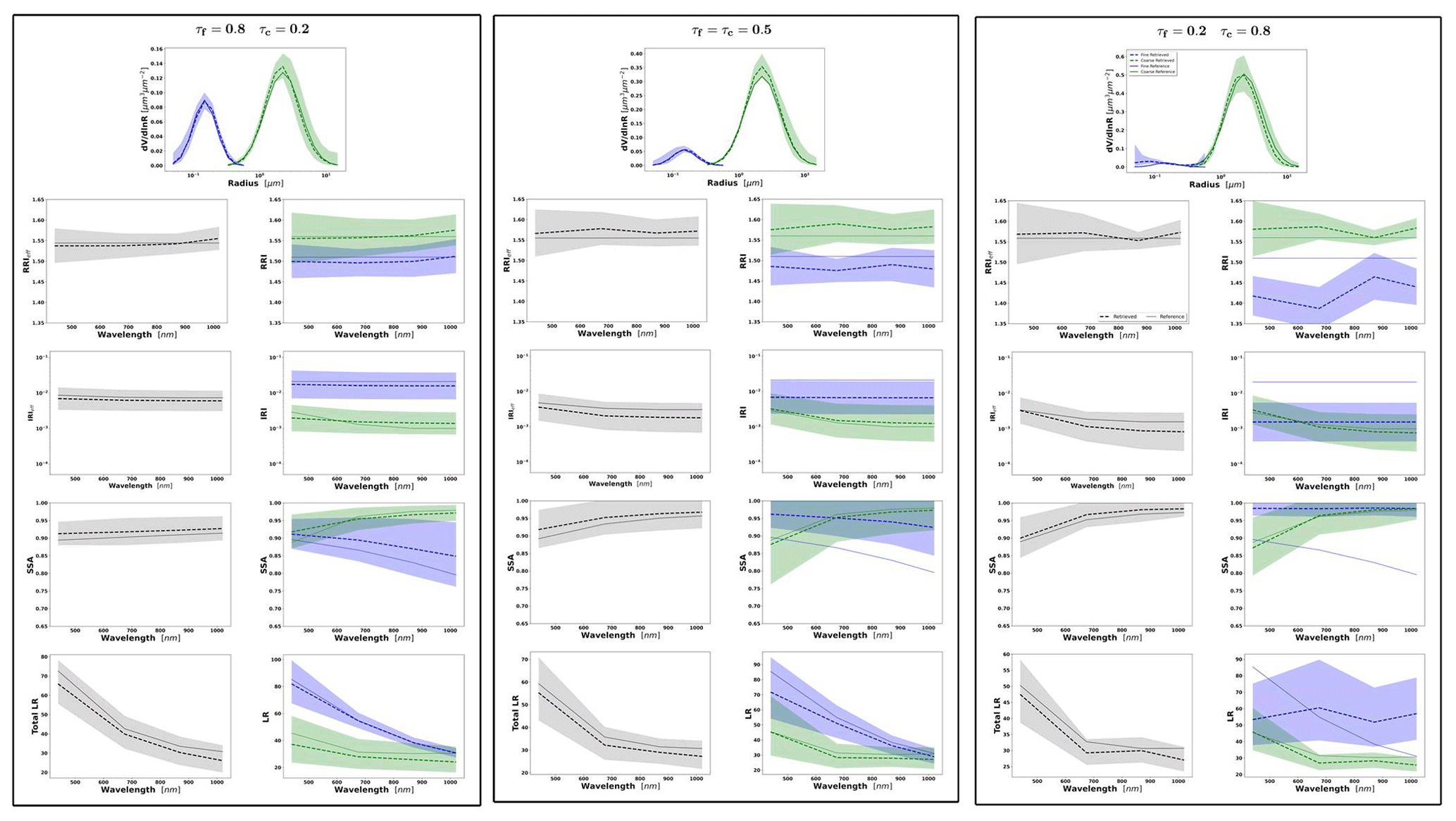
Figure 30 Aerosol properties retrieved from simulated sun/sky photometer data with assumed random noise and bias in AOD- and radiance-simulated data for BB–Dust for τ(440)=1.0. Retrievals after adding positive bias +0.01 in AOD and +5 % in radiances are represented in both cases. The solid lines are the simulated properties (SD, RRI, IRI and SSA), and the dashed lines are the retrieved parameters. The shaded area indicates the systematic error estimated by the GRASP algorithm.

On the other hand, in this section, some illustrations for the lidar ratio are also provided in order to demonstrate how the retrievals and the error estimates are affected by the bias in the measurements. Figure 30 illustrates the lidar ratios in this situation of mixed aerosol. The retrieval results and estimation of the LR errors are rather satisfactory, with exceptions of low AOD cases, mainly in the case where the fine mode has only a very minor presence (of τ_f=0.2 and τ_c=0.8). Also, it should be emphasized that the errors estimated for total SSA and refractive index (RI) are rather adequate, while in Sect. 4.1, where only random errors were considered, the results showed some apparent underestimations.

4.2.3 Effects of measurement bias in the retrieval of mixed aerosol properties from observations of radiometers in combination with lidar

This section considers the same example as in Sect. 4.2.2 and analyses the effects of measurement biases in the synergy retrieval using coincident measurements from the sun/sky photometer and lidar measurements. At the same time, the results are presented for the most practical situation when both random and biased values are present in the measurements and accounted in the error estimates.

Figure 31 shows the results for the example of BB–Dust described in the previous section for τ(440)=1.0 and assumes the presence of both bias and random noise in all the synthetic measurements for AOD, radiometers and lidar. As can be seen, the results of these different tests illustrate the positive influence of using radiometer and lidar synergy. The error estimates seem to be rather accurate too. For example, the most notable enhancement is in the lidar ratio accuracy, especially when the fine mode is the smallest, i.e. for the case with the following: τ_f=0.2 and τ_c=0.8. This behaviour was also seen by Lopatin et al. (2013), who explained that these were expected results, since the lidar ratio has a high sensitivity to the lidar signal. Nevertheless, we can see some improvements in the retrieval of complex refractive index using both lidar and photometer data.

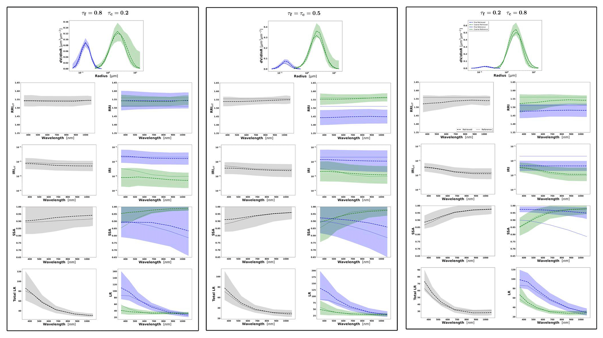
Figure 31 Aerosol properties retrieved from simulated sun/sky photometer and lidar data with assumed random noise and bias in AOD-, radiance- and lidar-simulated data for BB–Dust for τ(440)=1.0. Retrievals after adding positive bias +0.01 in AOD, +5 % in RAD and +0.2, +0.15 and +0.1 for each lidar wavelength at 355 nm, 532 nm and 1064 nm, respectively. The solid lines are the simulated properties (SD, RRI, IRI, SSA and LR), and the dashed lines are the retrieved parameters. The shaded area indicates the total errors estimated by the GRASP algorithm.

With regard to the accuracy of the error estimation, in Sect. 4.1, we have illustrated the retrieval of error estimates for LR and showed some apparent underestimation when only random errors were considered. Figure 31 illustrates an important improvement in the estimation of the errors, once both random noise and bias are considered and Eq. (31) is used for accounting the effect of the systematic component.

Thus, using the synergy of both instruments can provide more accurate retrievals of LR, and the error can be estimated rather accurately using the developed methodology for both aerosol components, even for an aerosol mode with a lower presence. Figure 32 illustrates the retrievals of the vertical aerosol profile in all three cases. The results show similar tendencies to Sect. 4.1.

Figure 32 Aerosol properties retrieved from simulated sun/sky photometer and lidar data with assumed random noise and bias in AOD-, radiance- and lidar-simulated data for BB–Dust for τ(440)=1.0. Retrievals after adding positive bias +0.01 in AOD, +5 % in RAD and +0.2, +0.15 and +0.1 for each lidar wavelength at 355 nm, 532 nm and 1064 nm, respectively. The solid lines are the simulated properties (SD, RRI, IRI, SSA and LR), and the dashed lines are the retrieved parameters. The shaded area indicates the total errors estimated by the GRASP algorithm.

4.3 Illustration and description of the correlation matrices

The values of non-diagonal elements of covariance provide important and interesting information about the retrieved parameters. For example, if the values ${\mathit{\rho }}_{i{i}^{\prime }}\ne \mathrm{0}$ are close to ±1, the similitude of the influences of the parameters a_i and ${\mathrm{a}}_{i^{\prime }}$ on the inverted measurements f^* may explain the large variances in the retrieval error for these parameters. Also, knowledge about ${\mathit{\rho }}_{i{i}^{\prime }}\ne \mathrm{0}$ is highly useful for the situation when several parameters from a set of simultaneously retrieved parameters a_i need be jointly used in the applications. This can be easily seen from Eq. (29). For example, let us consider the estimates of two parameters, a₁ and a₂, which have errors, Δa₁ and Δa₂, characterized by covariance matrix, as follows:

$$\begin{array}{}\text{(37)}& {\mathbf{C}}_{\mathrm{\Delta }}=\left(\begin{array}{cc}{\mathit{\sigma }}_{\mathrm{1}}^{\mathrm{2}}& {\mathit{\sigma }}_{\mathrm{1}}{\mathit{\sigma }}_{\mathrm{2}}{\mathit{\rho }}_{\mathrm{12}}\\ {\mathit{\sigma }}_{\mathrm{1}}{\mathit{\sigma }}_{\mathrm{2}}{\mathit{\rho }}_{\mathrm{12}}& {\mathit{\sigma }}_{\mathrm{2}}^{\mathrm{2}}\end{array}\right),\end{array}$$

where a is a vector defined as $\mathit{a}=({\mathrm{a}}_{\mathrm{1}},{\mathrm{a}}_{\mathrm{2}}{)}^T$. Correspondingly, if in the application one needs to use the characteristic m that is a liner function of $m=K_{\mathrm{1}}{\mathrm{a}}_{\mathrm{1}}+K_{\mathrm{2}}{\mathrm{a}}_{\mathrm{2}}$, then the variance ${\mathit{\sigma }}_m^{\mathrm{2}}$ can be obtained from Eq. (29) as follows:

$$\begin{array}{}\text{(38)}& \begin{array}{rl}{\mathit{\sigma }}_m^{\mathrm{2}}& ={\mathbf{KC}}_{\mathrm{\Delta }\mathrm{a}}{\mathbf{K}}^T\\ & =\left(\begin{array}{cc}{K}_{\mathrm{1}}& K_{\mathrm{2}}\end{array}\right)\left(\begin{array}{cc}{\mathit{\sigma }}_{\mathrm{1}}^{\mathrm{2}}& {\mathit{\sigma }}_{\mathrm{1}}{\mathit{\sigma }}_{\mathrm{2}}{\mathit{\rho }}_{\mathrm{12}}\\ {\mathit{\sigma }}_{\mathrm{1}}{\mathit{\sigma }}_{\mathrm{2}}{\mathit{\rho }}_{\mathrm{12}}& {\mathit{\sigma }}_{\mathrm{2}}^{\mathrm{2}}\end{array}\right)\left(\begin{array}{c}{K}_{\mathrm{1}}\\ K_{\mathrm{2}}\end{array}\right)\\ & =K_{\mathrm{1}}^{\mathrm{2}}{\mathit{\sigma }}_{\mathrm{1}}^{\mathrm{2}}+K_{\mathrm{2}}^{\mathrm{2}}{\mathit{\sigma }}_{\mathrm{2}}^{\mathrm{2}}+\mathrm{2}{K}_{\mathrm{1}}{K}_{\mathrm{2}}{\mathit{\sigma }}_{\mathrm{1}}{\mathit{\sigma }}_{\mathrm{2}}{\mathit{\rho }}_{\mathrm{12}}.\end{array}\end{array}$$

From this equation, the importance of the correlation coefficient ρ₁₂ is quite evident. Specifically, if ρ₁₂=0, then the variance ${\mathit{\sigma }}_m^{\mathrm{2}}$ is just a simple sum $K_{\mathrm{1}}^{\mathrm{2}}{\mathit{\sigma }}_{\mathrm{1}}^{\mathrm{2}}+K_{\mathrm{2}}^{\mathrm{2}}{\mathit{\sigma }}_{\mathrm{2}}^{\mathrm{2}}$. Therefore, the error propagation from Δa_i to Δm is straightforward, and only the values of the sensitivities $K_i^{\mathrm{2}}$ determine the contribution of Δa_i (decreasing or increasing) to Δm.

When ρ₁₂≠0, the situation is more complex. However, the estimation of the main tendencies can be simplified in some cases. For instance, in the following:

$$\begin{array}{}\text{(39)}& \begin{array}{rl}& \text{if}{\mathit{\sigma }}_{\mathrm{1}}^{\mathrm{2}}={\mathit{\sigma }}_{\mathrm{2}}^{\mathrm{2}}\text{and}{K}_{\mathrm{1}}=K_{\mathrm{2}},\\ & \text{then}{\mathit{\sigma }}_m^{\mathrm{2}}=\mathrm{2}{K}_{\mathrm{1}}^{\mathrm{2}}{\mathit{\sigma }}_{\mathrm{1}}^{\mathrm{2}}(\mathrm{1}+{\mathit{\rho }}_{\mathrm{12}}),\end{array}\end{array}$$

or

$$\begin{array}{}\text{(40)}& \begin{array}{rl}& \text{if}{\mathit{\sigma }}_{\mathrm{1}}^{\mathrm{2}}={\mathit{\sigma }}_{\mathrm{2}}^{\mathrm{2}}\text{and}{K}_{\mathrm{1}}=-K_{\mathrm{2}},\\ & \text{then}{\mathit{\sigma }}_m^{\mathrm{2}}=\mathrm{2}{K}_{\mathrm{1}}^{\mathrm{2}}{\mathit{\sigma }}_{\mathrm{1}}^{\mathrm{2}}(\mathrm{1}-{\mathit{\rho }}_{\mathrm{12}}).\end{array}\end{array}$$

From these equations, it can be seen that if the correlation coefficient ρ₁₂→1 or ${\mathit{\rho }}_{\mathrm{12}}\to (-\mathrm{1})$, then, depending on the case in Eqs. (39) and (40), ${\mathit{\sigma }}_m^{\mathrm{2}}$ can be close to zero or up to $\mathrm{4}{K}_{\mathrm{1}}^{\mathrm{2}}{\mathit{\sigma }}_{\mathrm{1}}^{\mathrm{2}}$. Therefore, knowledge about the non-zero correlation coefficients ${\mathit{\rho }}_{i{i}^{\prime }}\ne \mathrm{0}$ is very important for understanding how the error is propagated to derived parameters obtained from the primary set a.

In practical cases, when the derived parameter m is a function of a large number parameters a_i, the contributions to ${\mathit{\sigma }}_m^{\mathrm{2}}$ increasingly become very complex with the increase in the number of involved parameters a_i. Therefore, unfortunately, the general qualitative analysis, similar to the one demonstrated by Eqs. (38)–(40), becomes very difficult and often practically impossible. Nonetheless, as will be shown below, the visualization of the correlation matrices in Eq. (33) can be very useful for an analysis of the retrieval tendencies.

4.3.1 Retrieval of single-aerosol components from radiometer measurements

Figure 33 shows the correlation matrices of random retrieval errors for BB (spherical particles) and dust (nonspherical particles) for a conventional AERONET-like inversion. The first 22 parameters (22×22) represent the SD. This is followed by two blocks of 4×4. These two blocks are related to the RRI and IRI for four wavelengths (440 to 1020 nm). The last parameter is the sphericity fraction (1×1). The colours represent the values of the correlation coefficients, where the red colour denotes positive correlations, and the blue colour indicates negative correlations. The density of the colours indicates the values of the correlation coefficients changing from zero (the white colour) to dense red or blue colours corresponding to values of 1 and −1 accordingly.

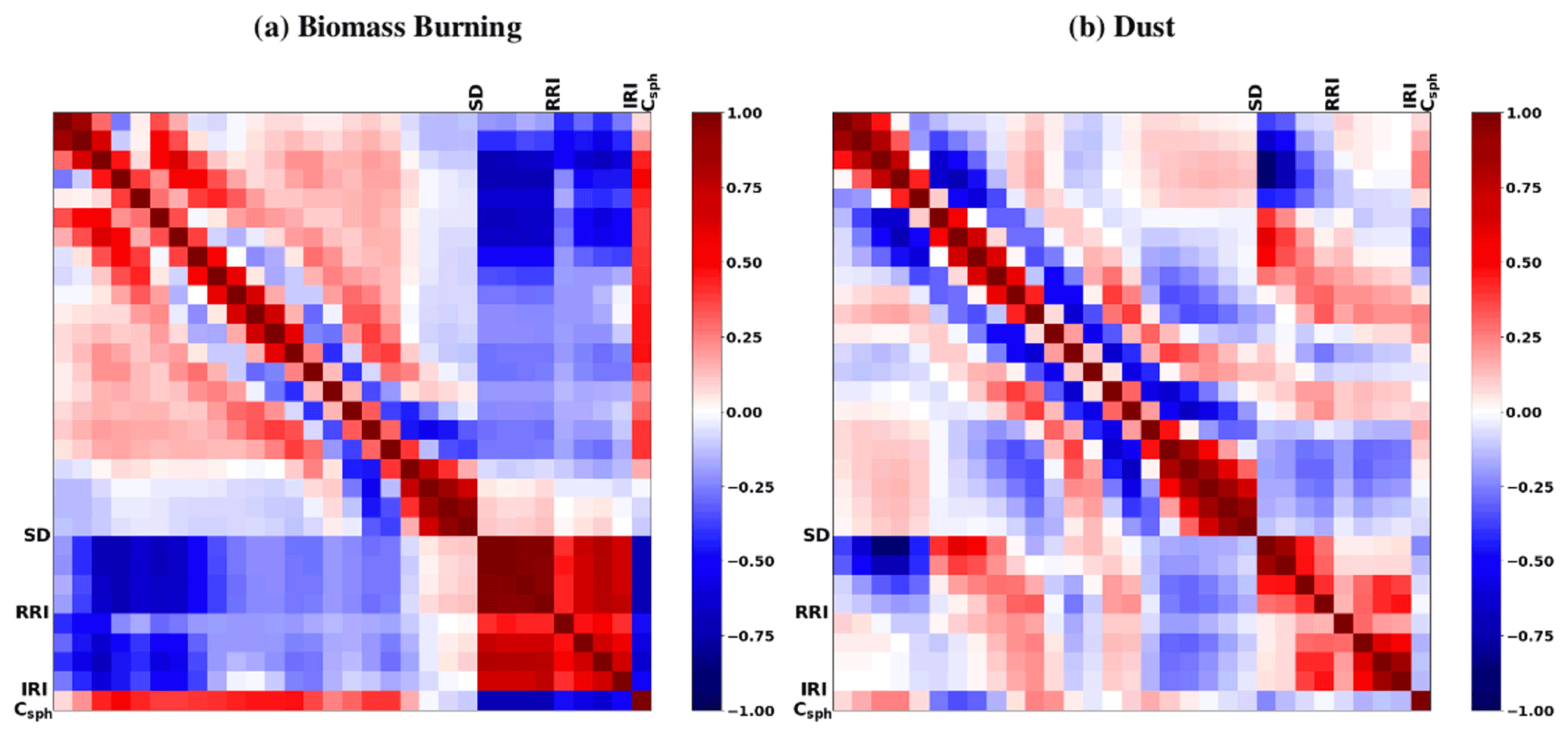
Figure 33 Correlation matrices of the estimated errors for aerosol retrieval from sun/sky radiometer observations (a) for biomass burning aerosols and (b) for desert dust using the GRASP algorithm. The values close to 1 or −1 mean stronger correlations between the properties, positive or negative, respectively.

The correlation for biomass burning case is shown in Fig. 33a. As can be seen, in general, size bin retrievals have a rather moderate correlation between them, though large positive correlations between the retrieval errors in neighbours can be observed. This is more evident for size bins at the smallest and largest particle sizes. This indicates that the size distribution values for those sizes have a tendency to be overestimated or underestimated together, which can mostly be explained by the use of the typical smoothness constraints imposed on the size distributions. The errors in RRI and IRI are negatively correlated with the SD parameters. The correlations seem especially pronounced between RRI and the values of the size distribution for the fine mode. Correspondingly, the overestimations of the size distribution values may tend to be accompanied by an underestimation of RRI, and vice versa. The errors in the fraction of spherical particle seem to show a positive correlation with the SD retrieval errors. This correlation is more evident when there is a fine-mode-dominated aerosol, since the scattering of fine-mode particles has a quite similar shape for spheres and spheroids. Therefore, when there is fine-mode domination it is more difficult to differentiate between spheres or spheroids. The positive sign of the correlation can be explained by the fact that extinction cross sections for the equivalent radii are a bit higher for spheroids. Thus, a higher percentage of spheres can be optically compensated by an increase in the volume concentration without a big impact in the total residual. The fraction of the spherical particle shows a negative strong correlation with the errors in the refractive index. Strong positive correlations can be seen between the spectral values of RRI. The positive correlations are present but lower between spectral values of IRI. As already noticed, this likely relates to the use of the rather strong smoothness constraint of the spectral variability in RRI and a weaker constraint of the spectral variability in IRI in the retrieval (Dubovik and King, 2000). The essential positive correlation can also be noticed between errors in RRI and IRI.

Figure 33b shows the correlation matrix for the retrieval of dust aerosol. The structure of the correlation for SD exhibits some differences compared to the BB case. Specifically, the positive correlations between the neighbouring size bins for the smallest and largest particle sizes are even more pronounced. Also, somewhat stronger negative correlations can be seen in the intermediate-sized ones. The strong negative correlation between RRI and SD retrieval errors remains only between concentrations of very small particles and the values of RRI at shortest wavelengths. The notable positive correlation is present only between the spectral values of RRI at the shortest wavelengths and between the spectral values of RRI at the longest wavelengths. At the same time, overall, the correlation of retrieval errors in both RRI and IRI, between themselves and with other parameters, decreases compared to the case of BB. The errors in the fraction of the spherical particle for the dust case correlates much less with the errors in the other parameter compared to BB case. This can be explained by the fact that the light scattering of large particles is significantly more sensitive to the deviation in aerosol particles from spheres compared to spheroids than the light scattering of fine fraction particles (Dubovik et al., 2006). Therefore, when coarse particles dominate, the discrimination between spheres and spheroids becomes more evident.

Thus, the analysis of the correlation matrices itself provide very useful insight that helps to understand and interpret retrieval results. For example, such artefacts as the appearance of tails (unrealistically high concentrations) at extremes of the size distribution have been noticed and widely discussed (Dubovik et al., 2002a; Dubovik et al., 2006; Torres et al., 2014). Such retrieval artefacts as the underestimation of RRI accompanied by an overestimation in the size distribution of very fine particles has been widely discussed in studies by Dubovik et al. (2000); Dubovik et al. (2002b, a). These artefacts were strongly reduced by accounting for the particle nonsphericity of desert dust particles (Dubovik et al., 2002b; Dubovik et al., 2006), but nonetheless the less-pronounced appearance of such artefacts remains in AERONET-like retrievals (Torres et al., 2014, 2017). These artefacts are clearly related to the above-observed presence of the strong negative correlation between the values of RRI and the size distribution of very fine particles. It should be noted that the presence of high correlations is an indication that adding information about one of the correlated parameters should improve the retrieval, not only for the constrained parameter itself but also for the parameters that strongly correlated with this parameter. For example, the addition of polarimetric observations to the traditional set of AERONET observations results in a clear improvement in the retrieval of RRI and the size distribution of very fine particles (Li et al., 2009; Fedarenka et al., 2016). Indeed, the degree of linear polarization is known to be very sensitive to the amount and especially the RRI of fine particles (Dubovik et al., 2006). This is why the addition of polarimetric observations helps to reduce the correlations between the errors in RRI and size distribution of fine particles and helps the overall improvement in the retrieval accuracy of these particles.

4.3.2 Retrieval of mixed aerosol components from radiometer measurements only

In this section, the correlation matrix for bicomponent aerosol retrieved from the synthetic observations of sun/sky radiometers of two aerosol mixtures is illustrated in Fig. 34 for BB–Dust and Urban–Dust. The structure of this matrix consists of 25 parameters related to the SD that are separated into two blocks, with 10 parameters for fine mode and 15 parameters for coarse mode. The following four blocks of 4×4 are related to the RRI and IRI of fine and coarse modes at four wavelengths. These blocks are followed by a single value of the sphericity fraction.

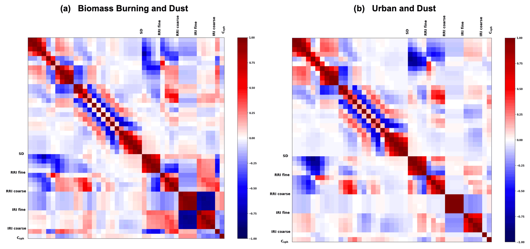
Figure 34 Correlation matrices of the estimated errors for mixed aerosol retrieval from sun/sky radiometer observations (a) for the mixture of biomass burning and dust aerosols and (b) for the mixture of urban and dust aerosols using the GRASP algorithm. The values close to 1 or −1 mean stronger correlations between the properties, positive or negative, respectively.

The area of the correlation matrix that contains SD, RRI, IRI and the sphericity fraction is quite similar to the correlation matrix obtained for aerosol AERONET-like retrieval. The main difference is the separation into two modes, since strong negative correlations can be observed between the corresponding parameters of the fine and coarse mode. For example, strong negative correlations can be observed between IRI fine and coarse mode. These correlations mean that overestimating the amount or absorption of one aerosol mode is likely compensated by underestimation of the amount or absorption of another aerosol mode. Another interesting anticorrelation can be observed for the last three bins of SD fine mode and the first three bins of SD coarse mode. Actually, both volume distributions have these three bins in common. This overlapping zone is never easy to properly separate for the code, but at the same time, it coincides with a local minimum value of most size distributions found in the real retrievals.

4.3.3 Retrieval of mixed aerosol properties from measurements of radiometers in combination with lidar

Figure 35 shows the correlation matrix for the case when the bicomponent aerosol retrieved from synthetic observations for the sun/sky photometer and lidar of aerosol mixtures is given. In the figure, the different blocks are identified. The first 25 parameters represent the SD that are separated into two blocks, with 10 parameters for fine mode and 15 parameters for coarse mode. The following four blocks of 7×7 are related to the RRI and IRI of fine and coarse modes at seven wavelengths. These blocks are followed by a single value of the sphericity fraction. The two last and largest blocks of 60×60 parameters each correspond to the AVP values of the two modes given at 60 different altitudes.

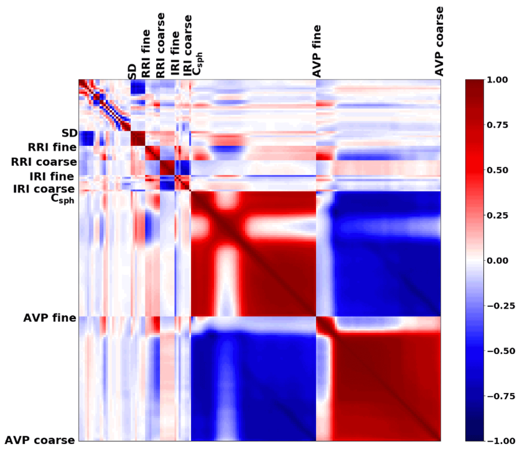
Figure 35 Correlation matrices of the estimated errors for aerosol retrieval from joint sun/sky radiometer and lidar observations for a mixture of urban and desert dust using the GRASP algorithm. The values close to 1 or −1 mean stronger correlations between the properties, positive or negative, respectively.

The area of the correlation matrix that contains SD, RRI, IRI and the sphericity fraction is quite similar to the correlation matrix described in the previous section, considering that the aerosol mixture retrievals are from AERONET-like observations only.

As expected, the block of the correlations of AVP retrieval shows strong negative correlations between the errors in the retrieved parameters of fine and coarse mode. Thus, an overestimation of one mode is highly correlated with an underestimation of another AVP mode. Furthermore, strong positive correlations can be observed between AVP values corresponding to the same fine or coarse mode, i.e. the AVP values of each mode have tendency to be simultaneously overestimated or underestimated. This is related to the limited sensitivity of the used lidar data for distinguishing the contributions of different modes and also to the use of smoothness constraints on vertical variations in AVP of each fraction. On the other hand, a near-zero correlation can be seen for AVP parameters at altitudes with a significant presence of one or both aerosol components. Correspondingly, there is a high sensitivity of both lidar and radiometer observations to the aerosol parameters at those altitudes. It should be noted that all the above-discussed retrievals suggested from the analysis of the correlation matrices were actually observed in the retrievals from real data, as discussed by Lopatin et al. (2013, 2021).

4.4 Illustration of the GRASP error estimates with real observations

This section illustrates the GRASP error estimates performance for the retrieval from real data. For that purpose, the lidar and sun/sky photometer measurements collected at the Aeroparque (34^∘33^′51^′′ S, 58^∘25^′02^′′ W) and Villa Martelli (34^∘33^′21^′′ S, 58^∘30^′23^′′ W) stations in Buenos Aires, Argentina, have been used. These instruments are part of the LALINET (Latin America Lidar Network; Guerrero-Rascado et al., 2016) and AERONET networks. Both sites are located in an industrialized city dominated by continental and urban/industrial aerosols and are affected during winter and spring by biomass burning from the north and centre of the country and neighbouring countries (mainly Brazil). The Aeroparque station is located at the Jorge Newbery International Airport within the city limits. This station does not have a co-located sun photometer, but its location is 7 km from the Villa Martelli station where the sun photometer is installed. On the other hand, the Villa Martelli station is found in the limits of Buenos Aires in a highly populated and industrialized area.

Observations from two different biomass burning events in Argentina were selected for the illustrations. Specifically, 3 d were chosen with different aerosol loads and SZA. The lidar range-corrected signals (RCSs) corresponding to each event are shown in Fig. 36. They have been calculated from the lidar signal, with background and dark current corrections and multiplied by the height squared. In addition, the back-trajectories calculated from the HYSPLIT (Hybrid Single-Particle Lagrangian Integrated Trajectory; Stein et al., 2015; Rolph et al., 2017) models are presented in order to confirm where the air masses come from (Fig. 37).

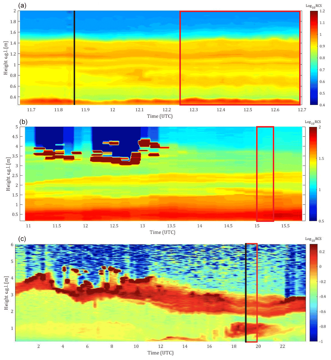
Figure 36 RCSs at 1064 nm in arbitrary units from Villa Martelli, Argentina, on 19 August 2014 (a) and 22 August 2014 (b) and from the Aeroparque station, Argentina, on 25 September 2017 (c). The two red lines indicate the analysed lidar data interval. The black solid line indicates the sun photometer measurements.

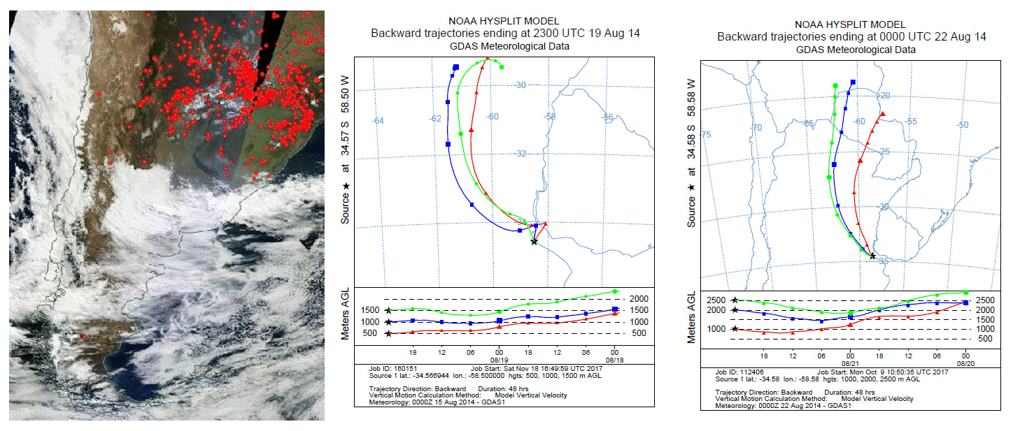
Figure 37 (a) Satellite image with hot spots corresponding to 22 August 2014 (NASA Worldview), (b) air mass back-trajectories for the Villa Martelli measurement site on 19 August 2014 and (c) air mass back trajectories for the Villa Martelli measurement site on 22 August 2014.

The two first cases selected correspond to an important event of biomass burning that occurred in the bordering countries to the north of Argentina in August 2014, particularly in the south of Brazil and Paraguay. It was detected in Buenos Aires between 19 and 23 August. For illustration purposes, the measurements corresponding to 19 August are used, which present a low aerosol load at 440 nm (∼0.11) and SZA >50^∘. Figure 36a indicated the presence of several layers of aerosols up to 1.5 km. The lidar measurements on 19 August were taken between 12:15 and 12:45 UTC, and the AERONET measurements correspond to 11:25 UTC. Figure 37 shows the HYSPLIT back trajectories that validate the source of the air masses. The measurements corresponding to 22 August are shown in Fig. 36b, where several layers of aerosol up to 3 km are observed. For this day, the aerosol load increases (AOD at 440 nm ∼0.31), and the SZA is <50^∘. The inversion was realized with the average lidar data between 15:00 and 15:20 UTC, and the AERONET measurements were considered at 16:59 UTC. The satellite image corresponding to 22 August (Fig. 37a) shows the presence of aerosols that extend from the north of Argentina towards the centre, passing through the province of Buenos Aires. Moreover, MODIS hot spots are detected in the satellite image. The source of the air masses can be validated from the HYSPLIT back trajectories (Fig. 37c). The last selected case corresponds to the biomass burning event on 25 September 2017, which occurred in the north of Argentina and in the bordering countries (Fig. 36c). In this work, lidar measurements from the Aeroparque station between 19:20 and 20:10 UTC and the AERONET measurements corresponding to 19:20 UTC, whose AOD value at 440 nm is 0.57 and SZA >50^∘, were used.

Figure 38 illustrates the retrieved columnar properties for each day obtained by GRASP from a combination of radiometer and lidar data and the comparison with the corresponding standard AERONET retrievals. The results provided by GRASP are represented in solid lines, with blue for the fine mode and green the coarse mode. Shaded areas represent the error provided by GRASP for each retrieved and derived property. Magnified plots represent the effective refractive index and total SSA for GRASP (black solid line) and AERONET (black dashed line). From the illustrations, one can see that almost all the GRASP-retrieved properties in the three cases present a good agreement with the AERONET retrievals.

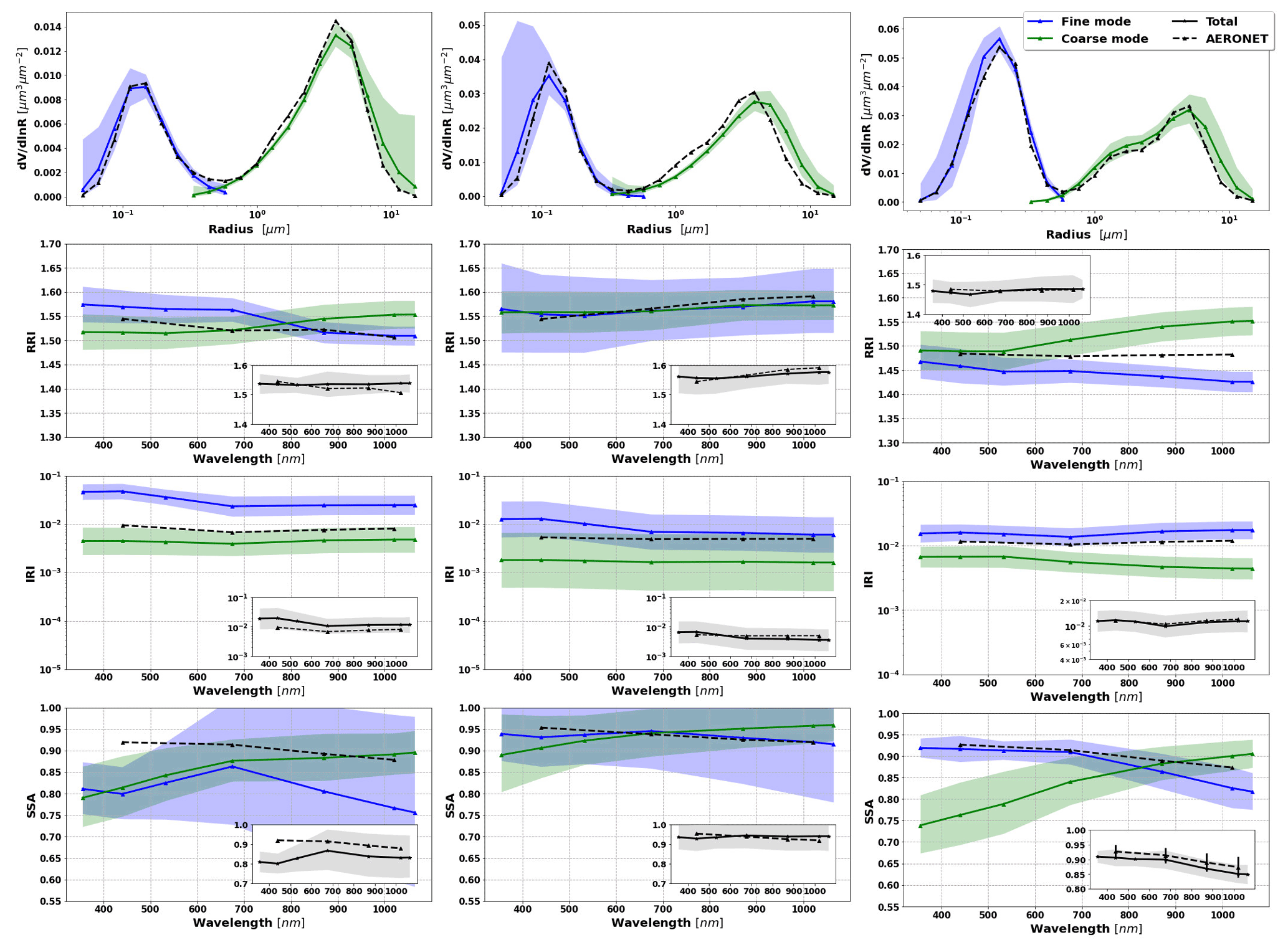
Figure 38 Comparison of columnar properties retrieved by GRASP from a combination of sun/sky photometer and lidar data and data retrieved conventionally by AERONET. SD, RRI, IRI and SSA retrieved by GRASP are shown in solid lines of blue (fine mode) and green (coarse mode). The shaded area in colours of blue and green represents the total error provided by GRASP, and black shaded areas are the uncertainties provided by AERONET. Magnified panels show the RI effective and total SSA provided by GRASP (black solid line) and AERONET (black dashed line). Their associated errors are represented in the grey shaded area for GRASP and with error bars for AERONET.

The error tendencies for SD that can be seen from Fig. 38 agree with those identified above in the present study and with results presented in previous sections and also with the results in some other works by Dubovik et al. (2000) and Lopatin et al. (2013). For example, the retrieval errors clearly increase at the extremes of SD. Moreover, one clear and known tendency can be mentioned. The size distribution shift towards higher radii in the three cases could be explained by the use of lidar data in the inversions that provide additional information at scattering angles of 180^∘ (Lopatin et al., 2013; Bovchaliuk et al., 2016; Benavent-Oltra et al., 2017). As seen in Fig. 38, these deviations, in almost all cases, are included in the error (shaded areas).

The errors in RRI, IRI and SSA were retrieved for each mode separately by GRASP, and they are significantly higher than the error for RRI, IRI and SSA of the total components. The effective RRI and IRI and the total SSA obtained by GRASP are in the middle of the retrieved values for fine and coarse mode separately. The total values shown in the magnified plots agree well with the RRI, IRI and SSA provided by AERONET.

On the other hand, the case corresponding to 25 September has an AOD >0.4 and SZA >50^∘, allowing us to have the uncertainty in the SSA provided by AERONET. Thus, in Fig. 38, for this particular case, we can observe the comparison of the uncertainty in SSA from AERONET and the SSA error provided by GRASP. Note that it is an advantage of GRASP that it provides the errors for each parameter in all the situations. Regarding the values of SSA and the tendencies of their variability, the results show that SSA is representative of biomass burning cases, namely that the values of SSA decreasing with the wavelength agree with AERONET climatology given by Dubovik et al. (2002a). As expected, based on the results of previous studies by Dubovik et al. (2000), Lopatin et al. (2013) and Tsekeri et al. (2017), the best agreements are obtained as the aerosol load increases. More specifically, we observe that the estimated errors in total SSA in the two first cases increase. This can be associated with unfavourable configurations of the observation. On 19 August the AOD at 440 nm is ∼0.11 (SZA is >50^∘) and on 22 August the AOD at 440 nm is ∼0.31 (SZA is <50^∘). Thus, the measurements in situations with a low amount of aerosol and with small SZA may not contain enough information to adequately retrieve the SSA (Dubovik et al., 2000; Lopatin et al., 2013; Torres et al., 2014). Therefore, the case of 25 September corresponds to the most favourable situation for realizing reliable aerosol retrieval, since the AOD at 440 nm value is >0.4, and SZA is >50^∘. Indeed, the GRASP and AERONET retrievals have the best agreement for this day.

Figure 39 shows the retrieved vertical distributions of fine and coarse modes. The vertical structure of the aerosols of different types is clearly discriminated and shows good agreements with the back-trajectory analysis for each day. Furthermore, the error estimates show good agreements with the previous results provided in the last sections for the simulated cases.

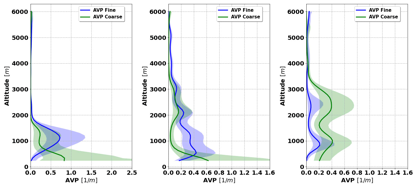
Figure 39 Retrieved aerosol vertical profiles (AVPs) by GRASP from a combination of sun/sky photometer and lidar data. The blue solid line represents the AVP fine mode and green the AVP coarse mode. The shaded areas correspond to the total error provided by GRASP.

Moreover, Fig. 40 shows the retrieved LR and their error estimates using the GRASP algorithm. The magnified plots show the total LR provided by GRASP (black solid line) and by AERONET (black dashed line). The associated errors are represented in shaded areas for GRASP. As can be seen, it is only possible to compare the values with AERONET retrieval for Fig. 40, which corresponds to higher aerosol load and SZA >50^∘ on 25 September 2017.

Figure 40 Retrieved LR by GRASP from a combination of sun/sky photometer and lidar data. The blue solid line represents the LR fine mode and green the LR coarse mode. Magnified plots show, with black solid lines, the LR provided by GRASP and, with dashed lines, the LR provided by AERONET. Their GRASP-associated errors are represented in shaded areas.

Thus, the retrieved parameters and error estimates from the GRASP application to the real data and their comparisons to the AERONET retrieval results showed an encouraging agreement between the columnar properties of aerosol. At the same time, GRASP provide the error estimates for the retrieved properties in both the fine and coarse mode and also for the total components. Moreover, GRASP has also the advantage of providing the dynamic error estimates in all configurations. As seen above, AERONET error estimates are only provided in some particular situations when the AOD at 440 nm is >0.4, and SZA >50^∘.

5 Conclusions

In this work, we reviewed the approach realized in the GRASP algorithm for estimating errors in the parameters retrieved from remote sensing observations. The employed approach relies on the rigorously realized concept of statistical estimations and tends to account for the propagation of both random and systematic errors. Then we evaluated the performance of the GRASP error estimates for aerosol parameters retrieved from ground-based observations. We considered AERONET-like retrievals from observations by sun/sky-scanning radiometers and GRASP synergy aerosol retrievals from joint observations by radiometers and lidar. GRASP generates the full covariance matrices that are expected to be used for generating error bars for retrieved parameters and provides an interesting insight for understanding retrieval tendencies. Therefore, we studied the quantitative reliability of the obtained covariance diagonal elements and analysed the structure of correlation coefficient of covariance matrices.

The performance of the GRASP estimates of error variances in the presence of random errors was evaluated in a series of numerical tests and illustrated the capabilities of the GRASP algorithm to provide rigorous estimates of dynamic retrieval errors. In the frame of these tests, the synthetic proxy observations perturbed by 300 random-noise-generated realizations were inverted using the GRASP algorithm. Then, the retrieved parameters were compared to those used for the generation of the synthetic data, and the obtained error estimates were compared with actual deviations in the retrieved parameters from assumed values. This analysis was realized for the synthetic observations for three different types of aerosols and for the mixture of them. Observations of dust were modelled using AERONET retrieval climatology at the Solar Village (Riyadh, Saudi Arabia) site. The AERONET retrieval climatologies from the African savanna (Zambia) and the GSFC (Maryland, USA) were used to simulate urban and BB aerosol observations, respectively. The Urban–Dust aerosols and BB–Dust mixture were considered for modelling the properties of mixed aerosols. For each observed aerosol type or mixture thereof, different aerosol loads were tested. First, we modelled observations of aerosols of only one type aerosol for τ(440)=0.3, 0.6 and 0.9. For aerosol mixtures, we also considered scenarios with different aerosol loads, while we present most of the illustrations of the situations with a large aerosol load (τ(440)=1.0, combining different aerosol loads for each mode τ_f=0.2 and τ_c=0.8, ${\mathit{\tau }}_{\mathrm{f}}={\mathit{\tau }}_{\mathrm{c}}=\mathrm{0.5}$ and τ_f=0.8, and τ_c=0.2). The data were perturbed by random noise before applying the retrieval algorithm. For all these simulations, the SZA at 75^∘ was used.

The tests evaluated the situations when only radiometer data were inverted, and then radiometer data were inverted jointly with coincident lidar data. Two GRASP retrieval set-ups were tested, where (i) the retrieval assumes that aerosol is composed of homogeneous particles, and parameters of only one aerosol component are retrieved, and (ii) then the aerosol is assumed to be an external mixture of two aerosol components, and the parameters of each component are retrieved separately. In the case when the lidar data were used, the vertical profiles of the concentration were also retrieved for each aerosol component. The illustrations for aerosol retrieval from all simulated data sets were provided, using both approaches. However, the full statistical analysis provided only the two conventional retrieval scenarios, i.e. AERONET-like, single-component retrieval from radiometric observations and GRASP bicomponent aerosol retrieval from combinations of radiometer and lidar data.

The results of the tests showed that the complete set of aerosol parameters for each aerosol component can be robustly derived with acceptable accuracy in almost all considered situations. The retrieval of bicomponent aerosol was evaluated using radiometer-only simulated measurements and then adding lidar observations. These tests allowed us to observe that, by using the synergy of two instruments, there are some improvements in the retrieval of the aerosol properties of each component of the observed aerosol mixture and in the estimations of the retrieval errors. The test for selected cases with different presences of different aerosol components (τ_f=0.2, τ_c=0.8 and τ_f=0.8, τ_c=0.2) showed that optical properties of the dominant mode can be retrieved in a significantly more accurate manner than expected. It is interesting to note that in all situations that use only radiometer data or add lidar-simulated measurements, properties such as total SSA and effective refractive index can be retrieved rather accurately, even in cases where the retrieval of the properties of each mode separately is questionable.

The results of the statistical tests with randomly generated noise showed that the GRASP error estimates, in most cases, are comparable to or exceed the actual errors by 20 % to 30 % and therefore can be safely used for assuring uncertainties in the actual retrieval products. In addition, the observation of typical error values was summarized for different situations and retrieval scenarios. Namely, the study confirmed that the detailed properties of aerosol mixtures can be rather reliably retrieved from a combination of radiometer and lidar data, provided that there is a sufficient amount of both aerosol components. For example, for the case when the total τ(440)=1.0 with a comparable presence of both components ${\mathit{\tau }}_{\mathrm{f}}\left(\mathrm{440}\right)={\mathit{\tau }}_{\mathrm{c}}\left(\mathrm{440}\right)=\mathrm{0.5}$, and SZA is 75^∘, the mean values for RRI errors are ∼0.05 for BB and urban and vary between 0.07 to 0.09 for dust, and IRI errors are around 60 % for BB, 75 % for urban and 50 % for dust. SSA errors vary between 0.024 and 0.061 for urban, 0.042 and 0.086 for BB and 0.04 and 0.009 for dust, showing a clear tendency to increase with the wavelengths for values of fine mode and decrease for coarse mode. However, even for this case, the separation of the LR values for both modes showed high uncertainties at short wavelengths, in particular for the fine mode, while the values of the total LR errors were found to be reasonable in the range of 20 % to 55 %. The relative error estimates for AVP for both aerosol mixture (Urban–Dust and BB–Dust) cases were ranging for fine mode between 50 % and 70 % and for coarse dust mode between 50 % and 55 %.

The effects of the systematic errors in the retrievals were also analysed in a series of limited dedicated numerical tests. The results of the tests were used for adjusting the GRASP retrieval estimates to the potential effects of the systematic errors. The results show enhancements of total error estimates from the assumption of bias in the equation of systematic components.

In addition to the evaluation of the error bar estimates and the effects of systematic errors, in this paper we illustrated and discussed the correlation structures of the error covariance matrices for all main considered retrieval scenarios. The results showed that analysis of the correlation structure can be very useful for understanding the observed retrieval tendencies and optimizing retrieval. For example, for conventional AERONET-like aerosol retrievals from radiometer data only, the strong negative correlation between errors is in the real part of the refractive index and size distribution values for small sizes. This agrees well with the tendency commonly observed in actual retrieval when the underestimations of the real part are coincident with the overestimation of the fine-mode size distribution. Also, the presence of a high positive correlation between the errors in the size distribution for extreme sizes and between the errors in the refractive index at different wavelengths agrees well with the known possibilities of possible overestimations of aerosol concentrations for very small or very large particles and joint overestimations/underestimations of the refractive value at different wavelengths. For bicomponent retrievals, strong negative correlations can be observed between nearly all corresponding parameters of the fine and coarse mode. This means, for example, that the overestimation of the amount or absorption of one aerosol mode is likely compensated by underestimation of the amount or absorption of another aerosol mode. The decrease in some of these correlations was observed when inverted radiometer data were inverted simultaneously with the lidar data. The high positive correlations were seen for the errors in the vertical profile of the fine and coarse concentrations, with the exception of the values for the altitudes where one or both of the aerosol modes had substantial loads. These and other less obvious, but quite interesting, correlation structures and tendencies can be identified using the analysis of the correlation matrix structure. Thus, the availability and analysis of not only the error variances but also the correlation patterns appear to be a useful and promising approach for optimizing observation schemes and retrieval set-ups.

Finally, the utilization of GRASP for deriving detailed aerosol properties and estimations of their errors was demonstrated for the coincident lidar and sun photometer observations from Buenos Aires, Argentina. The GRASP retrievals and the error estimates of the columnar aerosol properties were shown to be fully adequate in a comparative analysis with the aerosol products available from AERONET operational retrievals. The retrieval of the vertical profiles of fine and coarse aerosol modes showed results consistent with the expectation and the predictions of back-trajectory analysis.

Thus, the results presented in this work show promising potential for the utilization of GRASP-retrieved dynamic error estimates for the detailed retrieved aerosol parameters from measurements of ground-based radiometers and lidars, considering different geometries and the presence of diverse aerosol loads. These studies are expected to be completed in future by a more extensive analysis of the error estimates for such detailed parameters as vertical profiles of SSA and LR.