Biomass burning aerosol heating rates from the ORACLES (ObseRvations of Aerosols above CLouds and their intEractionS) 2016 and 2017 experiments

Aerosol heating due to shortwave absorption has implications for local atmospheric stability and regional dynamics. The derivation of heating rate profiles from space-based observations is challenging because it requires the vertical profile of relevant properties such as the aerosol extinction coefficient and single-scattering albedo (SSA). In the southeastern Atlantic, this challenge is amplified by the presence of stratocumulus clouds below the biomass burning plume advected from Africa, since the cloud properties affect the magnitude of the aerosol heating aloft, which may in turn lead to changes in the cloud properties and life cycle. The combination of spaceborne lidar data with passive imagers shows promise for future derivations of heating rate profiles and curtains, but new algorithms require careful testing with data from aircraft experiments where measurements of radiation, aerosol, and cloud parameters are better colocated and readily available.

In this study, we derive heating rate profiles and vertical cross sections (curtains) from aircraft measurements during the NASA ObseRvations of Aerosols above CLouds and their intEractionS (ORACLES) project in the southeastern Atlantic. Spectrally resolved irradiance measurements and the derived column absorption allow for the separation of total heating rates into aerosol and gas (primarily water vapor) absorption. The nine cases we analyzed capture some of the co-variability of heating rate profiles and their primary drivers, leading to the development of a new concept: the heating rate efficiency (HRE; the heating rate per unit aerosol extinction). HRE, which accounts for the overall aerosol loading as well as vertical distribution of the aerosol layer, varies little with altitude as opposed to the standard heating rate. The large case-to-case variability for ORACLES is significantly reduced after converting from heating rate to HRE, allowing us to quantify its dependence on SSA, cloud albedo, and solar zenith angle.

1 Introduction

Off the western coast of southern Africa, a semi-permanent, seasonal stratocumulus cloud deck occurs in a broad region of subsidence in the southeastern Atlantic Ocean (Zuidema et al., 2016; Gordon et al., 2018). A westward outflow from the African continent transports biomass burning (BB) aerosols out over the low clouds. The BB aerosols originate from fires in the continental interior, where they have been lofted through convective heating (Zuidema et al., 2016; Adebiyi and Zuidema, 2018).

Due to flaming burning conditions, the BB aerosols have a high black carbon content, contributing up to 10 % of the total aerosol mass (Redemann et al., 2021; Dobracki, 2021). With a single-scattering albedo (SSA) of approximately 0.83±0.03 at 550 nm (Cochrane et al., 2021), these aerosols absorb a significant portion of the incoming and reflected radiation. The direct interaction with radiation by scattering and absorption is known as the direct aerosol radiative effect (DARE).

Aerosol absorption induces diabatic heating of the layer, which has important consequences for atmospheric stability and dynamics. The free-tropospheric layer containing the aerosol is warmed, while the surface below is cooled, which stabilizes the low cloud deck. Observations indicate lower cloud top heights; higher liquid water paths; and optically thicker, brighter clouds when more shortwave-absorbing aerosols are present (e.g., Hansen et al., 1997; Dubovik and King, 2000; Kaufman et al., 2002; Johnson et al., 2004; Wilcox, 2010, 2012; Yamaguchi et al., 2015; Zuidema et al., 2016; Gordon et al., 2018). If the aerosols directly interact with the cloud below, the aerosol warming may facilitate cloud dissipation by reducing the relative humidity, along with altering the cloud microphysics (Hill et al., 2008; Diamond et al., 2018; Zhang and Zuidema, 2019; Mallet et al., 2020).

The aerosol layer in the southeastern Atlantic is also colocated with elevated levels of water vapor (Haywood et al., 2003; Adebiyi et al., 2015; Deaconu et al., 2019; Pistone et al., 2021), which have radiative impacts distinct from those of the aerosol layer. In addition, water vapor can also modulate the aerosol itself: Magi and Hobbs (2003) find that the aged smoke (older than 45 min) in the southeastern Atlantic is swollen (humidified) due to the water vapor.

The first step in understanding subsequent dynamic effects and cloud interactions is to determine heating rate profiles throughout the aerosol layer. In addition to the information required to determine DARE (i.e., aerosol and cloud properties), calculating heating rate profiles also requires accurate, detailed information on their vertical distribution.

Lidar instruments are specifically designed to penetrate through the atmosphere to obtain vertical profiles of atmospheric backscatter and extinction, including those specific to aerosols. When positioned on satellites, lidar instruments can provide aerosol extinction profiles for large spatial regions, which can be combined with additional observations that provide aerosol optical properties (e.g., Deaconu et al., 2019) or incorporated into climate models (Mallet et al., 2019; Tummon et al., 2010; Gordon et al., 2018; Adebiyi et al., 2015; Wilcox, 2010).

With current backscatter lidars, extinction profiles cannot be obtained directly due to the convolution of aerosol backscattering and extinction in the returned lidar signal. For example, the Cloud-Aerosol Lidar with Orthogonal Polarization (CALIOP) aboard the Cloud-Aerosol Lidar and Infrared Pathfinder Satellite Observation (CALIPSO) satellite measures the attenuated backscatter coefficients at 532 and 1064 nm, from which the extinction coefficient is typically retrieved based on modeled values of the extinction-to-backscatter ratio (also called the lidar ratio) inferred for each detected aerosol layer (Young and Vaughan, 2009). The depolarization ratio method (DRM) (Hu et al., 2007; Chand et al., 2009; Deaconu et al., 2017; Kacenelenbogen et al., 2019) also known as the opaque water cloud (OWC) method takes advantage of the CALIOP depolarization measurements and the transmission constraints provided by underlying low liquid water clouds to derive accurate measurements of the above-cloud aerosol optical depth (ACAOD) and the mean lidar ratio of the aerosol layer above the cloud (Liu et al., 2015).

High-spectral-resolution lidars (HSRLs) are likely to be included in future space architectures. Among other advantages, they will provide extinction profiles directly (Hu et al., 2007; Hair et al., 2008). This would be useful with the new concept of heating rate efficiency (HRE) first introduced in this paper (Sect. 5). It represents the heating rate at any altitude as obtained from aircraft observations per aerosol extinction coefficient, which, by contrast to the heating rate itself, varies little throughout the profile. It is possible that the HSRL-derived extinction profiles could be directly translated into aerosol heating rates for regions where HRE and downwelling irradiance are available.

To develop the HRE concept, we use a combination of in situ and remote sensing observations from 2 years of the ObseRvations of Aerosols above CLouds and their intEractionS (ORACLES) aircraft experiments (2016 and 2017). The aircraft is ideally suited for obtaining vertical information, which can be taken from varied instruments for different parameters. In situ measurements can provide profiles of water vapor, while aerosol extinction profiles can be provided by either overflights with the High Spectral Resolution Lidar 2 (HSRL-2) (Burton et al., 2018) or vertical profiles with the Spectrometer for Sky-Scanning, Sun-Tracking Atmospheric Research (4STAR; Dunagan et al., 2013; LeBlanc et al., 2020) instrument.

For nine cases (corresponding to those presented in Cochrane et al., 2021), we attribute the total heating of the layer to contributions from the aerosol, water vapor, and other atmospheric gases. We also examine the dependence of the aerosol heating rates and HRE on aerosol properties and cloud albedo – the same parameters that also modulate DARE (Cochrane et al., 2021). Section 2 of this paper describes the data and general methods of the heating rate calculations. Section 3 provides the results and discussion for heating rates segregated by absorber, while Sect. 4 describes heating rate results along an aircraft flight leg, known as a heating rate curtain. Section 5 introduces the new HRE concept, and Sect. 6 provides a summary.

2 Methods

2.1 Data

The NASA ORACLES project utilized the NASA P-3 aircraft for the 2016, 2017, and 2018 deployments, while the ER-2 aircraft was additionally deployed in 2016 to record high-altitude measurements (Redemann et al., 2021). Both aircraft were equipped with instrumentation to sample clouds and aerosols. The P-3 payload included both remote sensing and in situ instruments, while the ER-2 aircraft carried only remote sensing instrumentation.

To determine heating rates, we use a combination of measurements taken from the Solar Spectral Flux Radiometer (SSFR), 4STAR, and HSRL-2. SSFR is a system consisting of two pairs of spectrometers that measure the upwelling (nadir) and downwelling (zenith) irradiance between 350 and 2100 nm. The zenith light collector is mounted on an active leveling platform (ALP), which keeps the light collector level with the true horizon during flight. SSFR is radiometrically calibrated before and after the mission, with field calibrations performed throughout each deployment to keep track of instrument changes throughout the duration of the experiment (Cochrane et al., 2019). The 4STAR instrument measures aerosol optical depth (AOD) above the aircraft between 350 and 1650 nm, as well as provides column gas retrievals such as water vapor and ozone, aerosol intensive properties, and cloud properties (Segal-Rozenhaimer et al., 2014; Pistone et al., 2019; LeBlanc et al., 2020). The instrument is calibrated before and after the mission using the Langley method at the Mauna Loa Observatory (e.g., Schmid and Wehrli, 1995; LeBlanc et al., 2020). HSRL-2 provides vertical profiles of aerosol backscatter and depolarization at 355, 532, and 1064 nm wavelengths, along with aerosol extinction at 355 and 532 nm wavelengths, all of which are measured below the aircraft (Hair et al., 2008; Burton et al., 2018). In 2016, HSRL-2 was mounted on the ER-2 aircraft but transitioned onto the P-3 aircraft for 2017 and 2018.

A major benefit of aircraft campaigns is the flexibility to perform distinctive flight maneuvers in a way that optimizes measurements and retrievals for different instrumentation. In this work, we use two distinct flight patterns: stacked legs (so-called radiation walls) and vertical profiles (so-called square spirals) to derive (a) heating rate curtains and (b) heating rate profiles segregated by absorber, respectively. Figure 1 shows the locations of the radiation walls and spirals used in this study.

Figure 1 The location of spirals and radiation walls within the ORACLES study region. Spirals are shown as circles colored by the SSA retrieval (Cochrane et al., 2021) at 550 nm. Radiation walls are shown as black rectangles labeled by date. Please note that the date format in this figure is year month day.

Radiation walls, the traditional maneuver for radiation science flights, consist of vertically stacked legs flown in sequence along a fixed ground track. The stacked legs bracket the aerosol layer above and below, at the bottom of the layer (BOL) and at the top of the layer (TOL). For ORACLES, the BOL leg was located just below the aerosol layer and just above the cloud layer. The column AOD (spectral), ozone, and water vapor are measured by 4STAR, and spectral scene albedo is measured by SSFR. The TOL leg is above the aerosol layer and the cloud, from which HSRL-2 measures profiles of extinction at 532 nm. In addition to the BOL and TOL legs, several other legs were flown within the wall, for example below and within the cloud and within the aerosol layer. A full radiation wall often required over an hour to complete, and a square spiral was often included at one end of the radiation wall.

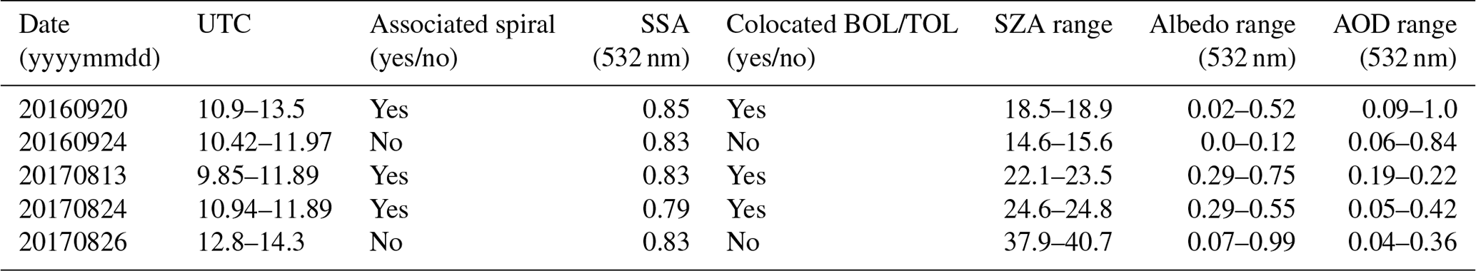
Since the radiation walls provide broad spatial coverage and allow us to sample varying cloud albedos and aerosol extinction profiles for the same aerosol plume, we use the radiation wall data to understand the impact of scene variability (i.e., aerosol loading and cloud albedo variability) on the aerosol heating rates. We do that by calculating heating rate curtains along the linear flight path, which require spiral measurements to be used in conjunction with AOD and scene albedo measurements from radiation walls (Table 1).

Table 1 Radiation wall case information. The last three columns refer to the BOL leg. SZA: solar zenith angle.

The downside of the radiation wall sampling is that it does not provide measurements throughout the aerosol layer. The new square spiral maneuver, described in detail in Cochrane et al. (2019), allows for multiple measurements to be taken throughout the vertical profile over a short time period (10–20 min depending on the vertical extent of the aerosol layer). From the measurements in the column (the layer that encompasses both the aerosol and the water vapor layer), absorption – and ultimately heating rates segregated by absorber (primarily water vapor and aerosols, detailed in Sect. 2.3) – can be derived.

Having the full column of measurements available from the spiral profiles led to the development of an aerosol optical property retrieval (SSA and the asymmetry parameter g, as detailed in Cochrane et al., 2021) that is directly tied to the irradiance measurements throughout the column. It is inherently difficult to retrieve these properties, since the aerosol radiative effects can be relatively small compared to the horizontal variability of cloud albedo. The spiral sampling strategy, however, reduces cloud and aerosol inhomogeneity effects while maintaining correlation of measured irradiances throughout the spiral to the ambient cloud field (Cochrane et al., 2019).

Table 2 RTM inputs for each spiral case (adapted from Cochrane et al., 2021). DU: Dobson unit.

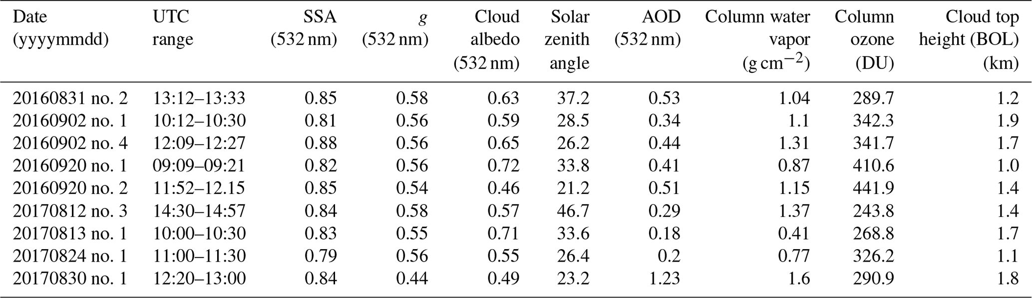
From all useable spiral maneuvers from ORACLES 2016 and 2017 (Cochrane et al., 2021), we combine the retrieved aerosol properties with the in situ measured water vapor content, 4STAR-derived spectral extinction (derived from the derivative of AOD along the vertical), and atmospheric-gas retrievals (Table 2). From these inputs, we calculate the vertical heating rate profiles for these cases. Since they are constrained by the total column absorption measured by SSFR, the heating rates are directly tied to the observations, ensuring consistency between aerosol properties, the water vapor profile, and the combined radiative effects of the atmospheric constituents (radiative closure). Since this is done spectrally, we can segregate by major absorbers to determine their relative contributions to the overall heating.

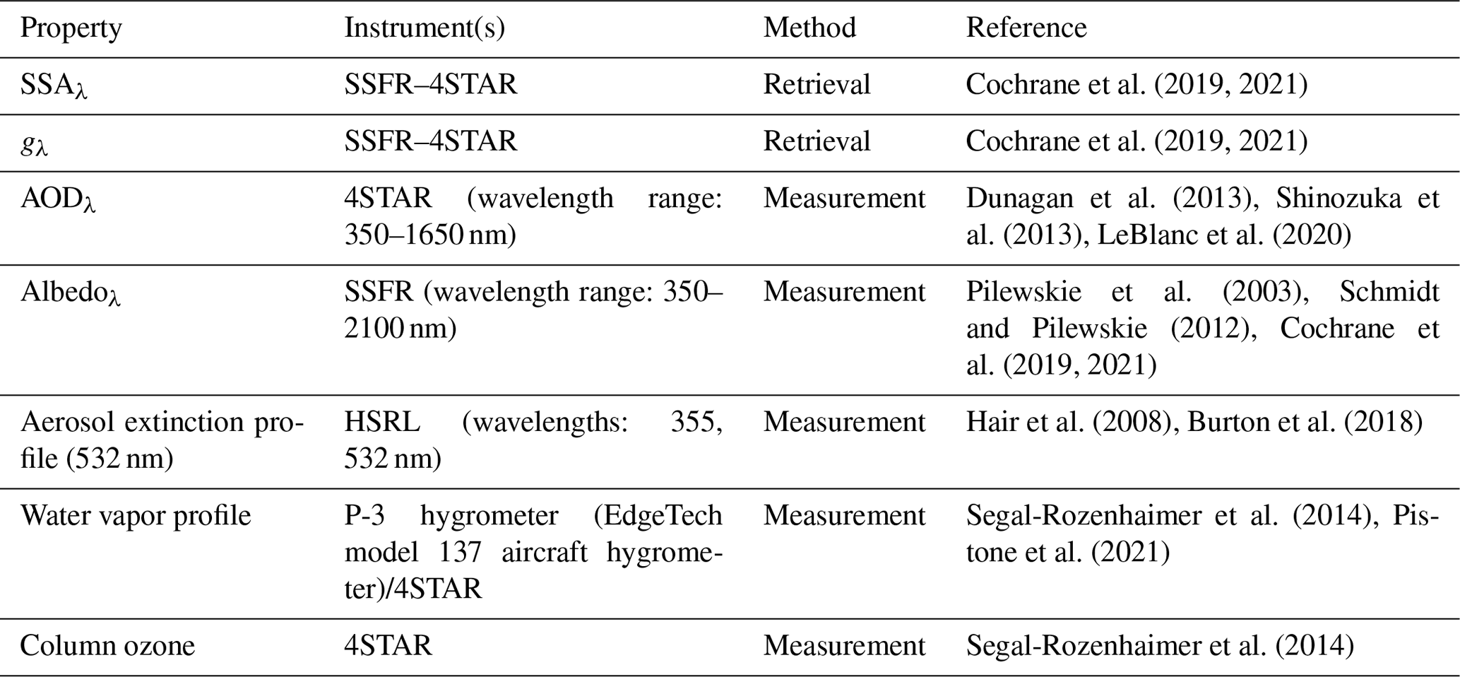
Table 3 Spiral profile and radiation wall heating rate calculation input parameters and their sources. The HSRL 532 nm extinction is used only for the radiation wall heating rates (curtains).

2.2 Heating rate calculations

To calculate heating rates for both the spiral profiles and radiation walls, we use the 1-dimensional (1D) radiative-transfer model (RTM) DISORT 2.0 (DIScrete Ordinate Radiative Transfer; Stamnes et al., 2000) with SBDART (Santa Barbara DISORT Atmospheric Radiative Transfer) for atmospheric molecular absorption (Ricchiazzi et al., 1998) within the libRadtran library (library for radiative transfer; Emde et al., 2016; http://libradtran.org, last access: 3 January 2022). Table 3 lists the input parameters and their sources required for the calculations. The general method is to segregate the absorption by strategically eliminating a single constituent for separate calculations (Kindel et al., 2011). First, we calculate the total heating rate from cloud top to well above the top of the aerosol layer, then remove a single atmospheric component from the profile (e.g., aerosols) and calculate the heating rate again. The difference between the two calculations provides the isolated heating rate for the individual component that was excluded in the second calculation.

The radiative-transfer calculations are performed in this manner rather than by calculating the heating rate of each component directly in order to maintain physical consistency. As incoming radiation travels through the atmosphere, less and less total radiation reaches lower altitudes. When there is a strong absorber present, such as an aerosol layer, the decrease of radiation with altitude is amplified, since the layer absorbs a significant portion of the incoming radiation. Calculating absorption (and heating) for a single component directly does not consider the attenuation by other constituents, potentially leading to an overestimation of the heating rates at altitudes below that of the absorbing layer.

We calculate the heating rate of a layer following the equation presented in Schmidt et al. (2021):

$$\begin{array}{}\text{(1)}& {\displaystyle \frac{\mathrm{\Delta }T}{\mathrm{\Delta }t}}={\displaystyle \frac{\mathrm{1}}{\mathit{\rho }{c}_p}}{\displaystyle \frac{\mathrm{\Delta }{F}_{\mathrm{net}}}{\mathrm{\Delta }z}}=\int {\displaystyle \frac{\mathrm{1}}{\mathit{\rho }{c}_p}}{\displaystyle \frac{\mathrm{\Delta }{F}_{\mathrm{net},\mathit{\lambda }}}{\mathrm{\Delta }z}}\mathrm{d}\mathit{\lambda },\end{array}$$

where ρ is the density; c_p is the constant-pressure specific-heat capacity of air; Δz is the layer thickness; and ΔF_net is the difference of the net irradiance at the layer top and bottom, i.e., the absorbed irradiance in that layer. Since the absorbed irradiance is a spectral quantity, the different wavelengths contribute varying amounts and must be integrated to find the total heating rate at each altitude. The heating rate is calculated at each layer altitude defined in the model (every 0.2 km for cloud top altitude of approximately 1 km < altitude <7 km and every 1 km for 7 km < altitude <12 km).

The RTM requires the spectral aerosol optical properties SSA and the asymmetry parameter g along with the vertical profile of aerosol extinction and the spectral albedo. SSA and g spectra are taken from the SSFR retrievals presented in Cochrane et al. (2021) and assumed to be vertically homogenous, since the retrieved values represent the entire layer. The spectral albedo measured by SSFR just above the cloud top defines the “surface” beneath the aerosol layer at the altitude of the cloud top. Aerosol extinction is either taken from HSRL-2 (for radiation walls) or derived from the 4STAR AOD profile (for spirals) and detailed in Sect. 2.3 and 2.4.

Atmospheric gases are defined by the standard tropical atmosphere included in the libRadtran package (Anderson et al., 1986). The water vapor and ozone profiles, however, are modified to reflect the specific conditions encountered during the time of the measurements. Specifically, due to the consistently high water vapor observed in the biomass burning plume (e.g., Pistone et al., 2021), the vertical distribution of the water vapor within the aerosol layer is first determined by in situ measurements taken by the P-3 hygrometer during the spiral profiles. Beyond the top of the aerosol layer (TOL), the values revert to those found in the standard atmosphere. The full column of water vapor (the water vapor path) is then scaled such that the total column (between BOL and the top of the atmosphere, TOA) is equal to the 4STAR retrieval at the lowest flight altitude. One example profile is shown in Fig. 2. Similarly, the ozone profile is scaled to the 4STAR ozone retrieval measured at BOL. For the spiral cases, the water vapor and ozone profiles are consistent with those used within the aerosol retrievals of Cochrane et al. (2021).

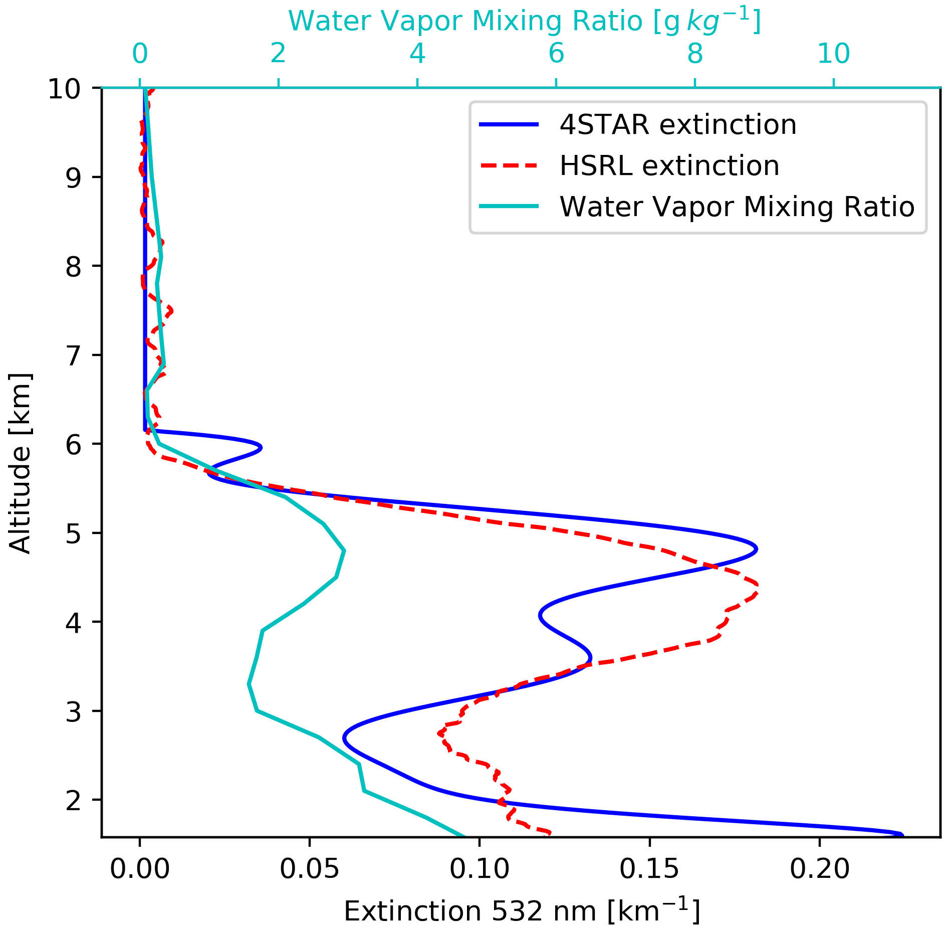
Figure 2 20160920 4STAR-derived 532 nm aerosol extinction profile (dark blue), averaged HSRL-2 532 nm aerosol extinction profile across the radiation wall (red dashed), and the water vapor content profile measured during the spiral profile (cyan). The 4STAR-derived extinction (532 nm) and the water vapor mixing ratio from the spiral profile is at a different location relative to the wall-averaged HSRL-2 extinction profile. Please note that the date format in this caption is year month day.

3 Heating rate segregation by absorber

The vertical profiles measured during the spiral flight patterns allow us to separate heating rates for different constituents beyond that of just the aerosol. This separation process relies on the principle that different atmospheric gases, aerosols, and water vapor absorb radiation in different wavelength ranges.

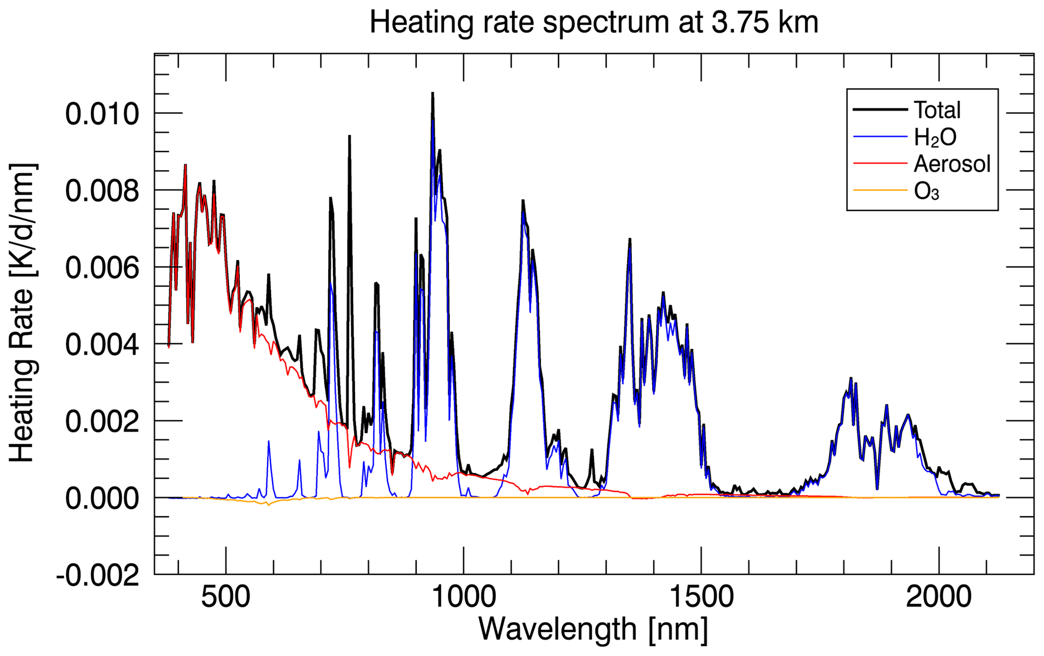
Figure 3 The total heating rate spectrum (black) shown along with individual heating rate spectra for aerosol, water vapor, and ozone at 3.75 km.

To separate the total heating into component-specific heating rates, we strategically remove components one by one and re-run the radiative-transfer calculations. For example, to determine the aerosol heating rate profile, we set the aerosol extinction profile to zero and calculate the heating rate profile. The difference between the total heating rate (where all constituents are included, i.e., the aerosol layer, water vapor, and ozone – all from measurements – as well as the libRadtran standard carbon dioxide and oxygen) and the total heating rate spectrum with the aerosol layer removed is the aerosol heating rate profile. The same technique is applied to each other constituent. Figure 3 illustrates the different heating rate spectra between the different components at one example altitude. This technique is appropriate where the removed component introduces a small perturbation to the downward flux, such as the cases presented here. However, very thick absorbing aerosol layers may induce shading effects on the downwelling flux, leading to a low bias in the calculated heating rates towards the bottom of the aerosol layer. This effect is minimal for our cases, but a modified technique should be considered for optically thick aerosol layers.

The aerosol extinction profile at each wavelength is obtained from the 4STAR measurements (derivative of AOD with respect to altitude), which provide the required spectral dependence throughout the profile. This is only possible when the profile of AOD measurements is available (i.e., from a spiral). This approach is consistent with the methodology used to retrieve the aerosol optical properties (SSA and g; Cochrane et al., 2019, 2021). Data conditioning is required such that the AOD profile decreases monotonically with altitude to eliminate any unphysical (negative) extinction values. These extinction profiles are consistent with those used in the aerosol property retrieval and have a 20 m vertical resolution; one example profile is shown in Fig. 2. The directly retrieved HSRL-2 aerosol extinction profile at 532 nm is close to the 4STAR-derived aerosol extinction profile. Any differences are due to the different location where these were acquired (wall vs. spiral) or due to the data conditioning applied to the 4STAR data.

Table 2 presents the input values for the required input parameters of the RTM heating rate calculations for each of the spiral cases.

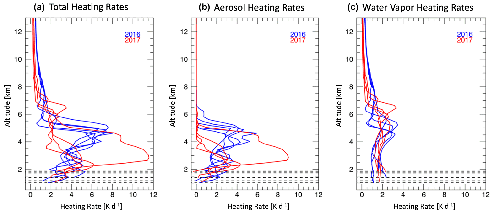
Figure 4 Vertical heating rate profiles for 2016 (blue) and 2017 (red) for (a) total, (b) aerosol, and (c) water vapor calculated from the spiral cases with valid aerosol SSA and g retrievals. Dashed lines indicate the bottom altitude for each profile.

Heating rates from spiral profiles

Total, aerosol, and water vapor heating rate profiles separated by year are presented in Fig. 4a–c. For the selected cases analyzed here, the aerosol plume was lower in altitude in 2017 than 2016, which can be seen in Fig. 4a (total heating rates) and 4b (aerosol heating rates). The peak aerosol heating rates were similar in both years, approximately 4–6 K d⁻¹, with the exception of one 2017 case for which the aerosol loading was significantly higher than other cases.

In 2016, the aerosol and water vapor layer were generally colocated in altitude (Fig. 4b and c), supporting the common assumption that aerosol and water vapor advect jointly from the continent. In 2017, by contrast, the primary aerosol loading resides below the free-tropospheric water vapor loading. The maximum water vapor heating (excluding the boundary layer) is between 2–4 K d⁻¹ at the specified solar zenith angles in both 2016 and 2017, though the 2017 water vapor heating rate peak is much broader than in 2016. These differences are possibly due to the differing locations and meteorological conditions, examined further in a campaign-wide analysis by Pistone et al. (2021).

Compared to Deaconu et al. (2019), who derived instantaneous heating rates from MODIS–POLDER–CALIOP (Moderate Resolution Imaging Spectroradiometer; Polarization and Directionality of the Earth's Reflectances) satellite instrumentation and the ECMWF ERA-Interim product from June–August 2008, we generally find lower peak aerosol heating rates: 4–6 K d⁻¹ vs. 9 K d⁻¹. This is likely due to differences in aerosol loading and vertical structure, since Deaconu et al. (2019) analyzed data much closer to the continent than any of our ORACLES cases. The instantaneous water vapor heating rate estimates, albeit at different solar zenith angles, are consistent: we calculate 2–4 K d⁻¹ compared to 3 K d⁻¹.

The water vapor contributions reported in this work as well as in Deaconu et al. (2019) are significantly larger than those in Adebiyi et al. (2015), who find that the maximum of the instantaneous water vapor shortwave heating rate is only ∼10 % of the maximum aerosol heating rate for clear skies near the island of St. Helena averaged over September–October: approximately 0.12 K d⁻¹ (water vapor) relative to 1.2 K d⁻¹ (aerosol). By contrast, our averaged maxima show the water vapor heating rate to be ∼60 % of the aerosol heating rate: 2.8 K d⁻¹ compared to 4.6 K d⁻¹. One reason is that the water vapor heating rates reported in Adebiyi et al. (2015) represent the difference between composite humidity profiles constructed from days with light and heavy aerosol loadings (AOD <0.1 and AOD >0.2, respectively) and rely on the positive correlation between aerosol and water vapor.

Comparing our results to other observations or model estimates previously reported in the literature (e.g., Marquardt Collow et al., 2020; Baró Pérez et al., 2021) is also challenging because heating rates depend on numerous parameters beyond spectral extinction profiles and single-scattering albedo: most importantly on the albedo of the underlying scene, layer depth, and vertical resolution, as well as variations in location (aerosol type) and solar zenith angle. Also, some studies report column-averaged rather than peak heating rates. This challenge is one of the motivations for the development of the heating rate efficiency (Sect. 5), which turns the heating rate (an extensive parameter proportional to the extinction) into an intensive quantity. If generally adopted, this new concept will allow for improved comparisons between studies.

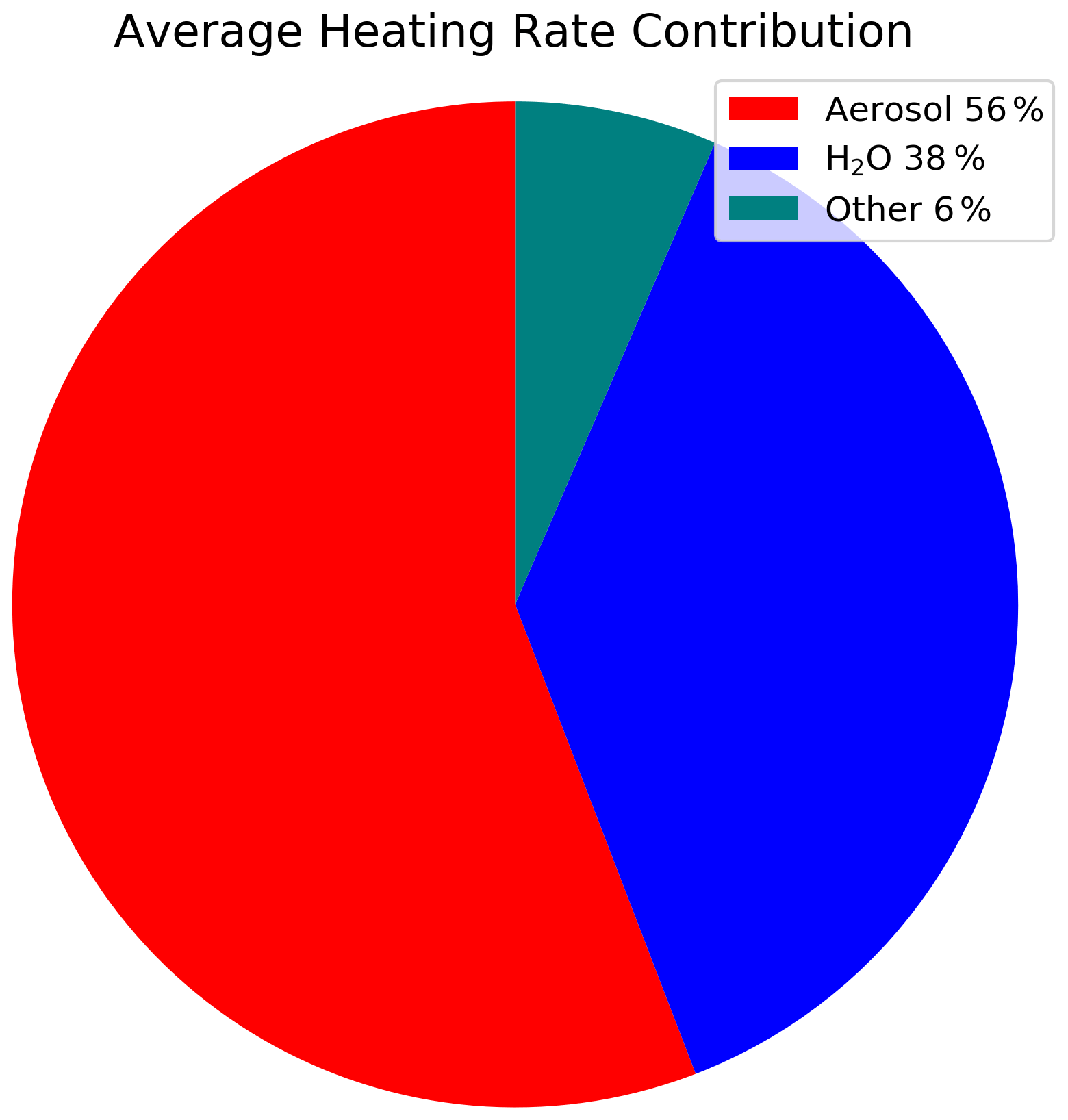
Figure 5 The case-averaged contributions to the total heating rate (column-averaged) from the nine spiral profiles mentioned in Table 3. The heating rate contribution of the category labeled “Other” is primarily gas (ozone, oxygen, and carbon dioxide) absorption.

Nevertheless, we first calculate the traditionally reported column-averaged heating rate (from cloud top to the top of the aerosol layer). Figure 5 shows the breakdown of the column-averaged total heating rate into its individual components, averaged for all cases. As expected, the largest contribution of heating stems from the aerosol (55.7 % of the total), followed by that from water vapor (37.5 %).

4 Heating rate dependence on scene parameters: heating rate curtains

For the radiation walls, we calculate heating rate curtains to examine the relative dependencies of the aerosol heating rates on AOD and the underlying albedo. This requires (a) aerosol optical properties and the water vapor profile (both obtained from a spiral retrieval and held constant); (b) the SSFR-measured albedo spectra, the AOD spectra, and column ozone retrievals from 4STAR, all of which are measured from the BOL leg of the radiation wall; and (c) aerosol extinction profiles at 532 nm of the full aerosol layer measured by HSRL-2 from the TOL leg (Table 2). Cases for which these criteria were not met were excluded from analysis. As mentioned above, radiation walls were typically accompanied by a spiral at one end. The spiral provides the aerosol optical properties along with the water vapor profile, while the colocated BOL and TOL legs provided the horizontal aerosol and cloud variability. Unfortunately, the spatial colocation is of little help, since the time lag between sequential sampling of the TOL and BOL legs is large enough that the cloud field is likely to change. In addition, some radiation walls included TOL and BOL layers that were not perfectly colocated and/or for which there was not an associated spiral that produced a valid aerosol retrieval.

Therefore, it was important to find a way to examine the heating rate dependence on the scene variability without knowing the albedo and AOD spectra underlying a specific aerosol extinction profile. We therefore assessed the dependence statistically by considering (1) the albedo variability and (2) AOD. For (1), we used the collection of measured spectra along the BOL leg, regardless of whether the BOL and TOL legs were colocated. From that, we created five representative albedo spectra for the heating rate calculations: the minimum, maximum, mean, and mean ± 1 standard deviation of the data collection. For part 2, we pursued a similar approach with the HSRL-2 extinction profiles from the TOL leg, which provide the vertical distribution of the aerosol. We paired this with the 4STAR-derived AOD from the bottom of the spiral (or from the leg-averaged BOL retrievals if a spiral was not available) as the basis for spectral extrapolation, which maintains spectral consistency across all heating rate calculations, as well as with the aerosol property retrievals. It should also be noted that for the two cases with no useable spiral, the aerosol optical properties were set to the ORACLES mean SSA and g spectra for the 2016 and 2017 deployments (Table 3 of Cochrane et al., 2021), and the water vapor profiles (and 4STAR column water vapor for scaling) are obtained from the closest spiral of the day regardless of whether there was a valid aerosol retrieval.

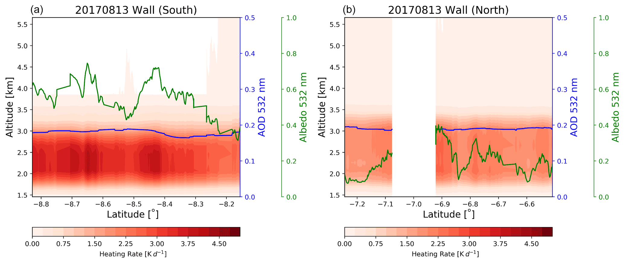
Figure 6 Heating rate curtains calculated using HSRL-2-measured extinction for the 20170813 radiation wall (shown here in separate plots: north in b and south in a). Peak heating of ∼4.8 K d⁻¹ occurs between 2 and 3 km. The underlying albedo, shown at 532 nm in green, is significantly higher on the left plot than the right (i.e., further south), contributing to higher aerosol heating rates. AOD, shown at 532 nm in blue, does not vary significantly across the wall. Missing results between −7.08 and −6.51 are due to in-cloud sampling that replaced above-cloud albedo measurements and serve as the break point between northern and southern ends of the wall. Please note that the date format in this figure and caption is year month day.

For each radiation wall, we calculate aerosol heating rates for extinction profiles from HSRL-2 along TOL, approximately one profile every 5 s (interpolated from the 10 s resolution reported in the HSRL-2 data product), which is approximately every 0.005^∘ of latitude or longitude. We extend the 532 nm extinction measured by HSRL-2 to the entire spectrum using the representative 4STAR AOD spectra in the following manner.

1. Integrate HSRL-2 extinction β_ext to get AOD at 532 nm:

   $$\begin{array}{}\text{(2)}& {\text{AOD}}_{\mathrm{532}}^{\mathrm{HSRL}}\left(x\right)=\underset{\mathrm{BOL}}{\overset{\mathrm{TOL}}{\int }}{\mathit{\beta }}_{\mathrm{ext}}\left(z,x\right)\mathrm{d}z,\end{array}$$

   where x is the location and z is the height.

2. Compare ${\text{AOD}}_{\mathrm{532}}^{\mathrm{HSRL}}\left(x\right)$ (from TOL) with ${{\mathrm{AOD}}^{\prime }}_{\mathrm{532}}^{\mathrm{4}\mathrm{STAR}}$ (where ${\text{AOD'}}_{\mathrm{532}}^{\mathrm{4}\mathrm{STAR}}$ is either the spectrum measured at the bottom of the spiral or the average spectrum of the BOL leg), and rescale the entire 4STAR AOD spectrum by the ratio between them:

   $$\begin{array}{}\text{(3)}& {\text{AOD}}_{\mathit{\lambda }}^{\prime }={\text{AOD}}_{\mathit{\lambda }}^{\prime \mathrm{4}\mathrm{STAR}}\cdot {\displaystyle \frac{{\text{AOD}}_{\mathrm{532}}^{\mathrm{HSRL}}\left(x\right)}{{\text{AOD}}_{\mathrm{532}}^{\prime \mathrm{4}\mathrm{STAR}}}}.\end{array}$$

3. Take the rescaled AOD spectrum, and divide by HSRL-2 AOD to get rescale factors at each wavelength (R_λ=1 at 532 nm):

   $$\begin{array}{}\text{(4)}& R_{\mathit{\lambda }}\left(x\right)={\displaystyle \frac{{\text{AOD}}_{\mathit{\lambda }}^{\prime }}{{\text{AOD}}_{\mathrm{532}}^{\mathrm{HSRL}}\left(x\right)}}.\end{array}$$

4. Get extinction profiles at all wavelengths using the rescale factors:

   $$\begin{array}{}\text{(5)}& {\mathit{\beta }}_{\mathrm{ext},\mathit{\lambda }}\left(x\right)={\mathit{\beta }}_{\mathrm{ext},\mathrm{532}}\left(x\right)\cdot R_{\mathit{\lambda }}\left(x\right).\end{array}$$

   In this approach, we are making two implicit assumptions: (1) that the 532 nm extinction can be used as a proxy of the full extinction spectrum and (2) that the spectral shape of extinction does not vary with location or altitude. This may not be fully representative of the aerosol layer: for example, there could be different amounts of coarse-mode aerosol in various layers of the plume, and SSA is not necessarily constant with altitude (LeBlanc et al., 2020; Redemann et al., 2021; Dobracki, 2021). One possible method to refine assumption (2) would be to introduce an altitude-specific spectral extinction adjustment based on the HSRL-2 Ångström exponent product, which could be investigated in further studies.

Figure 6 shows one example of the aerosol heating rate curtains calculated using the HSRL-2 extinction profiles. The high resolution of HSRL-2 allows us to resolve the minor variations within the aerosol plume while providing sufficient data to analyze the aerosol layer statistically. For each case, the albedo, AOD, and the aerosol extinction profile vary across the wall, while the intensive aerosol optical properties are assumed to remain constant. For the case shown in Fig. 6, the thickest part of the aerosol layer occurs between 2 and 3 km, with higher heating rates to the south. Although AOD along the wall ranges only from 0.19 to 0.22 at 532 nm, the high variability in the albedo causes large differences in the heating rate values.

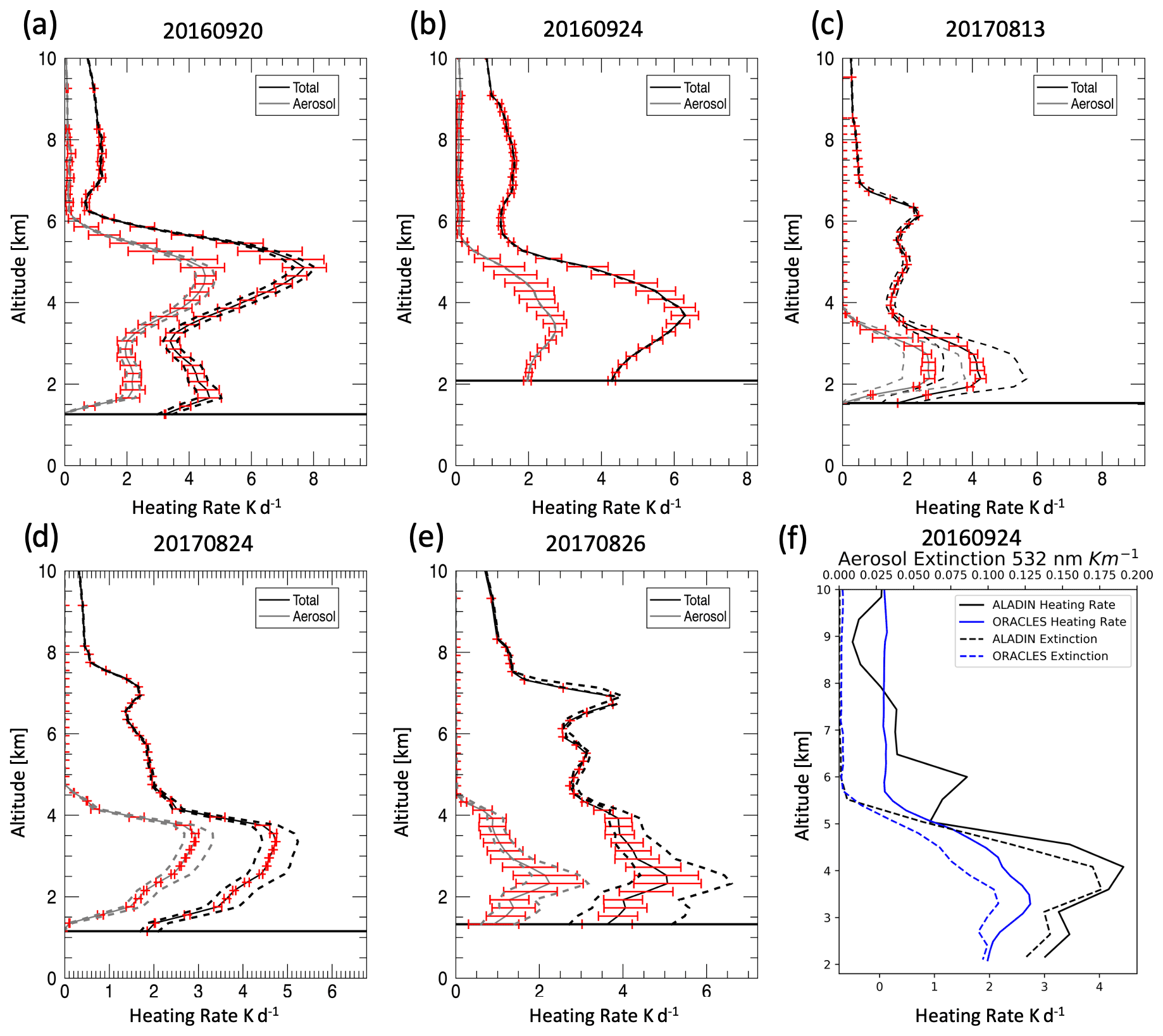
Figure 7 Mean vertical profiles for total (black) and aerosol (gray) heating rates across the radiation walls for five cases (a–e, calculated from HSRL-2 extinction profiles and SSFR–4STAR SSA and g values). The red error bars represent the variability due to changing extinction, while the dashed lines represent the variability due to changing albedo across the wall. The horizontal solid line indicates cloud top height. (f) Average aerosol heating rate profiles across the 20160924 radiation wall calculated from ORACLES vs. the ALADIN (Aire Limitée Adaptation dynamique Développement InterNational) climate model. Please note that the date format in this figure and caption is year month day.

The heating rate curtains provide enough data to examine the heating rate dependence on both AOD and the albedo along the wall for each of the cases. Each plot in Fig. 7 shows a thick solid profile (black) for the total heating rate and one for the aerosol heating rate (gray). These profiles represent the mean along the entire wall of HSRL-2 extinction profiles at the mean SSFR albedo value. The overlaid error bars represent the standard deviation (1σ) of the heating rate due to variable extinction for the mean albedo value. The dashed lines represent the mean for all extinction profiles for the lowest albedo and the highest albedo encountered during the wall.

In some cases, such as 20160920 (yyyymmdd; Fig. 7a) and 20160924 (Fig. 7b), the variation in AOD results in larger heating variation than caused by the changing albedo below the layer. In other cases, 20170813 (Fig. 7c) and 20170824 (Fig. 7d) the variation in heating due to changing albedo along the wall is greater than that introduced by AOD. In the 20170826 (Fig. 7e) case, the variation in albedo affects the total heating rate more than the AOD variation, while for the aerosol heating rate, AOD and albedo variation introduce approximately equal variations.

For every case, the mean total (aerosol) heating rate ranges between 4 and 8 K d⁻¹ (2–3 K d⁻¹). The aerosol heating values are similar to those found for the region by Keil and Haywood (2003; 2.3 K d⁻¹), Gordon et al. (2018; 1.9 K d⁻¹), and Wilcox (2010; 2.0 K d⁻¹). In contrast, we find slightly larger aerosol heating rate values than Tummon et al. (2010; 1 K d⁻¹) and Adebiyi et al. (2015; 1.2 K d⁻¹). Of course, we do not necessarily expect agreement with prior studies, since there are numerous differences between them such as different observational periods, locations, approach, and aerosol optical properties.

A direct comparison (in both observation location and time) for the 24 September 2016 radiation wall (Fig. 7f) between the ALADIN-Climate (Aire Limitée Adaptation dynamique Développement InterNational) regional model (Nabat et al., 2015) and our direct calculations shows a difference of approximately 1.5 K d⁻¹ in peak heating for the average aerosol shortwave heating rate profile, with the peak heating values from the ALADIN model slightly higher in altitude. The aerosol extinction profile from the ALADIN model is larger in magnitude than that of ORACLES. Likely the difference in extinction is the main driver in the differences between heating rates. The negative values between 7 and 10 km in the ALADIN profile may possibly come from differences in high-cloud properties between the two model simulations (Mallet et al., 2019).

5 Heating rate efficiency

Heating rate variability between cases, locations, and campaigns strongly depends on drivers such as extinction, cloud albedo, aerosol optical properties, and the vertical distribution. Unlike the related quantity DARE, which is usually studied at a single level such as the top of the atmosphere or the surface, heating rates extend throughout the entire column. In the past, it has been difficult to condense this into a single value to report and compare, leading to varying definitions and reported values in the literature (e.g., peak heating rate and column-averaged heating rate).

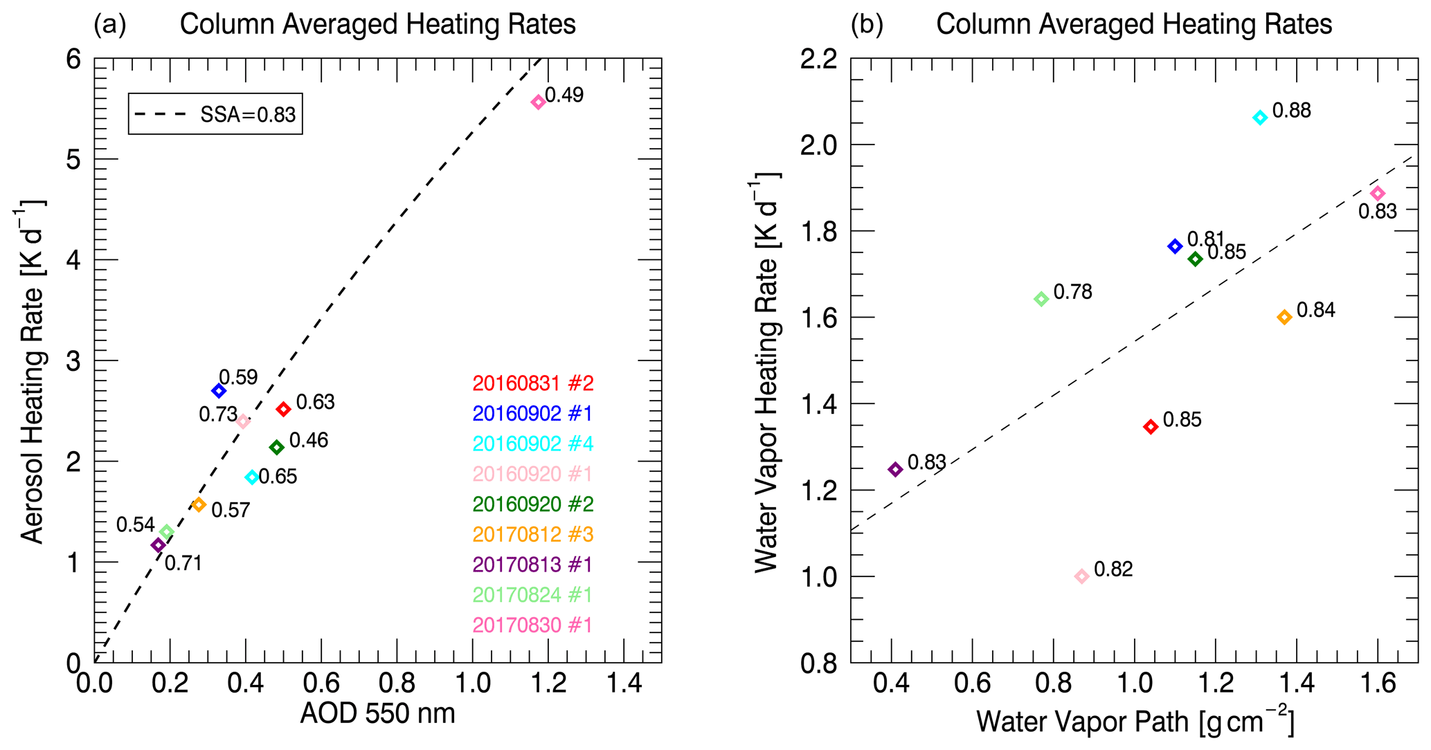
Figure 8 (a) Aerosol heating rate as a function of AOD at 550 nm. Column-averaged values from each spiral case are shown as colored points labeled by their 550 nm albedo value. The black dashed line indicates RTM calculations using mean SSA (0.83, 550 nm) and albedo (0.6, 550 nm) from all cases and a range of AOD spectra (ranging from 0 to 1.4 at 550 nm). (b) Water vapor heating rate as a function of the water vapor path. The gray dashed line is a simple linear fit to highlight the dependence. Cases are labeled by the 550 nm SSA value. The color coding in both (a) and (b) is denoted by the legend on (a). Please note that the date format in this figure is year month day.

The main drivers of the heating rates are key to understanding the origin of the variability and overcoming the factors that limit our ability to understand the heating rate variability. For aerosols, AOD is the most significant driver for the overall heating rate value. In Fig. 8a, the column-averaged aerosol heating rate for each spiral case is shown as a function of AOD at 550 nm, with some cases labeled by their 550 nm albedo value. As expected, aerosol loading, i.e., AOD, is the main driver of the heating rate, but a simple relationship is not expected because the vertical structure of the plume and its thickness vary from case to case. Still, the dependence can be confirmed with radiative-transfer calculations. We calculate aerosol heating rates as a function of AOD (black dashed line in Fig. 8a) for an SSA of 0.83, a g of 0.54, and an albedo of 0.60 (values listed for 550 nm; the full mean ORACLES spectra are used within the RTM). The vertical profile for these calculations was set to that of the 20160920 no. 2 spiral case.

For water vapor, the main controller of the heating rate is the water vapor path (the layer-integrated water vapor content), shown in Fig. 8b. Each case is labeled by the aerosol SSA value at 550 nm. The deviation of the individual cases from a linear relationship cannot be explained by the scene albedo at the water vapor absorption bands, since the dependence (not shown) is too weak. The most plausible explanation is therefore the vertical distribution of the water vapor. From Fig. 8a and b, we can see that layer heating by water vapor dominates over aerosol-induced heating up to a mid-visible aerosol optical thickness of about 0.25 (for a case with a water vapor path of ∼1.2 g cm⁻², SSA = 0.83).

From Fig. 8a, we can see that the variability in AOD between cases overwhelmed any signal from the smaller heating rate drivers such as SSA and albedo. The problem is that the variability of AOD and its vertical distribution are intertwined. To isolate the vertical distribution of the aerosol extinction coefficient from its column integral, we divided the heating rate at any given altitude z by the aerosol extinction coefficient, rather than working with the column-averaged heating rate as in Fig. 8 and in previous studies. We named this “intensive” parameter the relative heating rate efficiency, borrowing from relative aerosol forcing efficiency (Redemann et al., 2006), which is also independent of the aerosol loading. HRE is defined as the following:

$$\begin{array}{}\text{(6)}& \text{HRE}\left(z\right)={\displaystyle \frac{{\text{HR}}_{\mathrm{aerosol}}\left(z\right)}{{\mathit{\beta }}_{\mathrm{ext}}\left(z\right)}}\cdot \left({\displaystyle \frac{\mathrm{1}}{F^{\downarrow }\left(z\right)}}\right),\end{array}$$

where HR_aerosol is the aerosol heating rate profile; β_ext is the aerosol extinction profile at 532 nm; and F^↓ is broadband downwelling, spectrally integrated from 350–2100 nm. The units of HRE are (K d⁻¹) $/$ (1 km²) $/$ (W m⁻²).

The normalization by the incident broadband irradiance at any given altitude was included in the definition to account for the changing SZA and self-dimming (related to AOD) of the layer as we step further down into it. Using HRE instead of HR provides an alternate way to examine the dependence of aerosol heating on SSA, albedo, and SZA. Figure 9 shows an example of the vertical profile of the aerosol heating rate, extinction, and HRE, which clearly shows that HRE for the aerosol two sub-layers (at 2 and 4.5 km) is rather stable and comparable between the two layers, despite the variable extinction and heating rate profiles.

Figure 9 Vertical profiles of HRE, aerosol heating rate, and aerosol extinction at 532 nm. The vertical resolution defined in the model for which these calculations are performed is set to every 0.05 km for altitude <7 km and every 1 km for 7 km < altitude < 12 km.

To examine the dependencies of the heating rate efficiency on its drivers, we used the extinction profile, SSA retrieval, and measured cloud albedo for one spiral case (20160920 no. 2) as a reference and determined the HRE variation for changes in SSA, cloud albedo, and SZA. The SSA spectrum changes relative to the reference case are determined through the co-albedo, where the reference case is scaled to range from 0.01 to 0.24 at 532 nm. The scaled co-albedo (1-SSA) spectra are then translated back into SSA for input into the RTM. The cloud albedo spectrum changes relative to the reference case are obtained via cloud retrievals based on the reference albedo spectrum and then varying the retrieved cloud optical thickness to modulate the spectral albedo (for more details, please see Appendix A.3.2 in Cochrane et al., 2021). While SSA and cloud albedo were varied in the same way for the nine cases, the extinction profiles, water vapor profile remained case-specific.

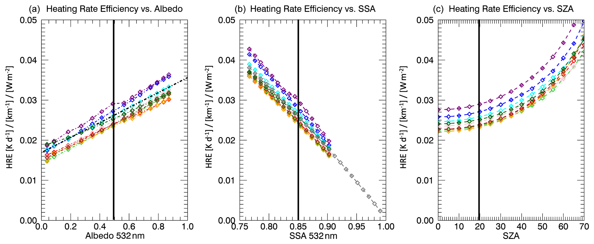
Figure 10 The profile-median HREs for varying aerosol vertical profiles as a function of (a) albedo, (b) SSA, and (c) SZA. The individual colored sets of calculations represent the different aerosol loading and vertical distribution measured during the nine different cases. The albedo spectra, aerosol optical properties, and SZA are consistent for each set of calculations (indicated by the black line), where SZA for both (a) and (b) is set to 20^∘, the albedo is set to 0.5 for (b) and (c), and SSA is set to 0.85 for (a) and (c).

Figure 10 shows the dependence of HRE on its main drivers. We can see that HRE (in contrast to layer-averaged heating rate) varies little from case to case and that its variability is tightly constrained by the albedo and SSA. It increases with increasing cloud albedo, consistent with the finding of Adebiyi et al. (2015). The same finding would be true for any bright surface (not just a cloud), although more complicated spectral dependencies would have to be considered. The black dashed line indicates the mean fit line, which extends from albedo values 0 to 1. From the fit line, it is apparent that HRE increases by approximately a factor of 2 across the full albedo range from 0 to 1. This can be understood intuitively, considering that the layer at an albedo of 1 is essentially illuminated “twice” – from the top and from the bottom. Of course, the heating of the layer is not exactly doubled, since the illumination from the bottom (the upwelling) is less than from the top (the downwelling) due to the partial attenuation of radiation.

Figure 10b shows that HRE decreases with increasing SSA. This is expected, since an increasing SSA indicates less absorption (relative to scattering), leading to lower heating rates. The gray symbols (calculated for the widened SSA range for one case only) show that HRE goes to 0 as SSA goes to 1 (purely scattering, no absorption). Decreasing SSA from 0.9 to 0.8 almost doubles HRE, which is also expected. It should be emphasized that the clear and easy-to-interpret dependence of HRE on the albedo and SSA could not have been achieved with the previous concepts of the layer mean or maximum heating rate. However, the benefits of the HRE concept also have a limit in that the extinction, SSA and albedo all have a spectral dependence, which is important to consider when deriving an inherently broadband quantity such as layer heating. In addition, one needs to consider the dependence of the heating rate on the solar geometry. Figure 10c shows that HRE increases as a function of SZA, with a sharp increase at the higher SZAs (lower sun elevations). This is due to the increase in path length through the aerosol layer as the sun moves towards to the horizon.

Figure 10 demonstrates the utility of HRE and highlights the effectiveness of the parameter for reducing the complexity of heating rates. At the albedo value of 0.5, an SSA of 0.85, and a 20^∘ SZA (location of the black lines in Fig. 10), HRE is 0.025 (K d⁻¹)/(km⁻¹)/(W m⁻²) with a standard deviation of only 0.002, approximately 8 % in relative terms. This small variability shows that HRE could be used to translate extinction profiles in the region directly into aerosol heating rates if mid-visible cloud albedo and SSA are also known. In other words, the variability in extensive parameters (e.g., extinction) is higher than intensive parameters (e.g., SSA and g), and therefore, regionally and seasonally defined HRE are useful. If available for a specific region, the HRE concept would allow for a direct translation from mid-visible extinction to heating rate, provided that the downward irradiances are available through either observations or radiative-transfer calculations. Of course, if SSA varies appreciably within the layer, that dependence may have to be made explicit. Alternatively, if in the future the absorption coefficient were available at sufficient accuracy in addition to the extinction coefficient, HRE could be redefined to normalize by the absorption coefficient, thereby accounting for the SSA vertical dependence.

6 Summary and discussion

Observations from the ORACLES 2016 and 2017 experiments allow us to introduce a method of determining heating rate profiles as directly as possible by linking the heating rates to SSFR-measured irradiance profiles. The spectrally resolved irradiance measurements and the derived column absorption allowed for the separation of heating rates by absorber, most importantly the separation of water vapor heating from aerosol heating. We found that for many cases, the water vapor heating rate is nearly as large as the aerosol heating rate, on average 38 % compared to 56 % of the total heating (respectively), highlighting the large influence of the distribution of atmospheric water vapor on the total heating rate distribution – even for optically thick aerosol layers. We also found that layer heating by water vapor coincident with aerosol dominates over aerosol-induced heating up to a mid-visible aerosol optical thickness of about 0.25 (for one case with a water vapor path of ∼1.2 g cm⁻², SSA = 0.83).

Analyzing the dependence of the heating rate on the driving parameters (AOD, albedo, and SSA) showed that the primary parameter affecting the aerosol heating rate is AOD and to a lesser extent the cloud albedo and aerosol SSA. For the mean SSA spectrum encountered during ORACLES (i.e., SSA of 0.83 at 550 nm), the heating rate increases by ∼0.5 K d⁻¹ per 0.1 increase in aerosol optical depth (for an albedo of 0.6 at 550 nm). The heating rate variability, however, is highly case dependent because of the co-variability of the driving parameters.

The vertical distribution of the aerosol layer in relation to the underlying cloud also introduce variability from case to case that cannot easily be evaluated. The impact of the vertical distribution makes heating rates more difficult to generalize than other radiative effects, such as the direct aerosol radiative effect (DARE, Cochrane et al., 2021). The new HRE parameter, however, does show potential for such a generalization because it defines the heating rate per extinction coefficient. HRE, in contrast to the heating rate, has a clear dependence on albedo and SSA that could not have been determined through either maximum or layer-averaged heating rate concepts. By reducing the complexity of the convoluted relationship between heating rates and their drivers, the HRE parameter makes it possible to investigate the relationship between heating rates and other parameters besides the aerosol loading and extinction profile. In the future, the HRE relationships established in this work could be formalized into a general parameterization applicable for the ORACLES study region. However, it will be important to consider that this type of broadband generalization will require spectral dependencies of extinction, SSA, and albedo.

For one preliminary comparison between our calculations and the ALADIN regional climate model output, we found consistent peak aerosol heating rates. The heating rate curtains, calculated along radiation walls using HSRL-2 extinction profiles, can currently only be derived from aircraft observations. To arrive at a similar product from satellite retrievals, one would have to ensure that the heating rates are consistent with a radiative flux constraint (at the very least at TOA), in addition to filtering out cloud inhomogeneity effects. This will be relevant for planned space-borne missions.