the Creative Commons Attribution 4.0 License.
the Creative Commons Attribution 4.0 License.
 | 14 Nov 2022
ICE-CAMERA: a flatbed scanner to study inland Antarctic polar precipitation
Massimo Del Guasta
Studying precipitation at very high latitudes is difficult because of the harsh environmental conditions that limit the external activity of humans and instruments, especially in the polar winter. The direct monitoring of ice crystal habits and size distribution in Antarctic precipitation is important for the validation of the algorithms used for retrieving precipitation from ground-based and satellite-borne radar instruments and for the improvement of the climatological modelling of polar areas. This paper describes an automated device (ICE-CAMERA) specifically developed for the imaging, measurement, and classification of ice precipitation on the Antarctic high plateau. The instrument gives detailed information on precipitation on an hourly basis. The article provides a description of the device and its image processing software. Starting in 2014, the instrument has operated almost unattended all year round at Concordia station, Antarctica (75∘ S, 123∘ E, 3220 m altitude).
- Article
(8764 KB) - Full-text XML
- BibTeX
- EndNote


In Antarctica, the characteristics of ice precipitation depend greatly on the region. In coastal areas, precipitation is influenced by synoptic-scale features, such as cyclones and fronts (Bromwich, 1988). In the interior (>2500 m), a significant part of the precipitation falls in the form of small ice crystals (“diamond dust”, DD) under clear-sky conditions (Fujita and Abe, 2006). Snow particles over Antarctica are generally smaller compared to other regions of the world. The largest particles are found close to the coast, where more water vapour is available and where diameters up to 10 mm are recorded (Konishi et al., 1992), with particle shapes similar to mid-latitude ones (Satow, 1983). Most of the bigger particles are aggregates (some can be found in the dataset of Grazioli et al., 2022). More inland stations record snowflakes of much smaller sizes, ranging from particles smaller than 100 µm at the South Pole (Walden et al., 2003; Lawson et al., 2006) to hundreds of µm at other inland stations (Lachlan-Cope et al., 2001).
In situ measurements of precipitation are rare in Antarctica and are affected by large uncertainties. This is particularly true in the high plateau, where less than 20 cm of snow accumulates every year (Palerme et al., 2014). As a result, the global precipitation products that rely on these observations (i.e. the Global Precipitation Climatology Centre, GPCC; Schneider et al., 2017) have no coverage over this region. Other observational products – such as the Global Precipitation Climatology Project (GPCP; Huffman et al., 2001), which uses GPCC for bias correction over land – have relied on satellite-only precipitation estimates. Satellite products also face large uncertainties over cold regions such as Antarctica due to the insufficient sensitivity of sensors to detect and estimate precipitation signals, the complex surface emissivities, and a poor understanding of precipitation microphysics. Ground-based K-band radars (∼1 cm wavelength) are robust instruments successfully employed for studying precipitation in coastal Antarctic sites (Souverijns et al., 2017), but they are quite blind to the sub-millimetre ice particles encountered on the plateau due to the relationship D6 between the radar scattering cross-section and the particle diameter (D).
The satellite-borne radar CloudSat (Liu, 2008) did provide a quantum leap in observing ice in the Antarctic atmosphere (up to 82∘ S), but being a single-frequency radar (like K-band radars), the retrieval of precipitation quantities relies on many assumptions about the properties of particles, resulting in ±50 % uncertainties for IWC (Heymsfield et al., 2008). The microphysical assumptions (shapes and size distribution of particles) are the biggest causes of IWC, IWP, and snowfall rate retrieval uncertainty (Hiley et al., 2011; Wood et al., 2015). Moreover, CloudSat bins close to the ground cannot be used for precipitation retrieval, resulting in a severe underestimation of the contributions of diamond dust and blowing snow to the Antarctic snow balance (Palm et al., 2018). Despite these uncertainties, in the absence of ground validation, CloudSat data are now used as an independent dataset for the validation of precipitation models in Antarctica (Palerme et al., 2014, 2017). The direct observation and the continuous monitoring of the habits and size distribution of precipitation are therefore required in order to validate both precipitation models, CloudSat and radar algorithms, on the Antarctic plateau.
Disdrometers are robust in situ devices, increasingly used in Antarctic coastal areas (Souverijns et al., 2017; Bracci et al., 2022). They provide the size distribution and falling speed of hydrometers, but they give no direct information about the shape. The evolution of disdrometers into 2D disdrometers gave access to some shape indications about hydrometeors (Grazioli et al., 2014). A further evolution of disdrometers into imaging disdrometers, such as the Snowflake Video Imager (SVI) (Newman et al., 2009), provided realistic images of the crystals. Grazioli et al. (2017a), as part of a multidisciplinary field campaigns, deployed a multi-angle snowflake camera (MASC) to take photographs of individual snow particles. This instrument, representing a further advance in the field of imaging disdrometers, collects high-resolution stereoscopic photographs of snowflakes in free fall while they cross the sampling area (Garrett et al., 2012), thus providing information about snowfall microphysics (Praz et al., 2017). The optical structure of the imaging disdrometer and the MASC makes these instruments reliable in the presence of millimetre-sized hydrometeor precipitation. In Antarctica, their practical application is mostly limited to coastal zones where particles are coarse (e.g. MASC resolution is 33 µm).
The direct observation of inner Antarctic particles requires imaging techniques with a resolution of a few microns. Photographic studies of precipitation in the interior of Antarctica are quite rare, carried out primarily at the South Pole station (SPS) through Formvar replicas. In early works with Formvar, Hogan (1975) identified at SPS millimetre-sized columnar crystals and column and bullet rosettes in cloud precipitation and smaller (≅100 µm diameter) plate-like particles in clear-sky precipitation. Satow (1983), working with Formvar replicas on Mizuho Plateau, found prevalently single bullets and a combination of bullets. Long, solid column crystals were also found (with an air temperature range from −42 to −56 ∘C), with a mean length of 290 µm and a maximum length of 1.2 mm and with a mean aspect ratio of 18. Small (50–400 µm) hexagonal, triangular, scalene, and square plates were also observed. Kikuchi and Hogan (1979) collected Formvar replicas of DD in the summer at SPS, finding columnar crystals of 90 µm average lengths and plates as small as 50 µm in diameter. Ohtake and Yogi (1979) classified winter ice crystal precipitation in Antarctica under six categories. These included large rosettes, bullets and columns (millimetre-sized), thin hexagonal plates and columns (200 µm or less), and smaller crystals of various shapes, including triangular and polyhedral. Shimizu (1963) observed “long column” crystals in the winter at Byrd Station (80∘ S, 120∘ W). Size distributions of Antarctic DD in winter and spring were reported by Smiley et al. (1980) for particles larger than 50 µm: they observed the same ice crystal forms that were reported earlier. Walden et al. (2003) studied DD, blowing snow, and cloud precipitation at SPS in winter by collecting crystals on slides and analysing them using microphotography. In their study, columns with an average length of 60 µm and plates with an average diameter of 30 µm were found in DD. The direct observation of ice precipitation on the plateau was typically carried out by means of Formvar replicas and/or microphotography, but these techniques take time, are difficult to implement throughout the year, and are necessarily limited to short field campaigns and samples of very limited size. Designing automatic instruments for the continuous, photographic study of precipitation in such a harsh environment necessarily requires several compromises between the high resolution of microphotography and the robustness of outdoor optical instruments such as disdrometers. Lawson et al. (2006) worked at SPS in summer, using innovative Cloud Particle Imagers (CPIs), which replaced Formvar replicas. This technique allowed the automatic analysis of around 700 000 DD crystal images in terms of caliper size, aspect ratio, and other shape parameters. An automatic classification software based on shape parameters was used to categorise the images into nine simplified classes: small plates and spheroids, columns, thick plates, plates, budding rosettes, rosettes, complex with side planes, and irregulars.
Concordia International Station, located on the Dome-C (DC, 75∘ S, 123∘ E, 3220 m above sea level) is a special location to test new instruments for precipitation studies. Surface temperatures seldom exceed −25 ∘C in summer, whereas winter temperatures can reach −85 ∘C. The 3 m average wind speed is 3 m s−1 for Aristidi (2005) and 4.5 m s−1 (hourly averaged) for Argentini et al. (2014). The strongest winds (up to 15 m s−1, hourly averaged) blow from the continental regions. These winds are due to gravity flows from the inner plateau regions south of Dome C and are more often observed during the winter, especially in coincidence with warming events. The circulation at the surface during the summer is affected, especially in the daytime, by the synoptic circulation. In summer, the wind speed oscillates during the day, with values increasing (by a few m s−1) in the afternoon when a convective layer develops, leading to the increase of the wind speed (Argentini et al., 2014). Relative humidity relative to ice is typically around 55 %–85 % (Genthon et al., 2022). In these conditions, precipitation of ice crystals can be studied by simply collecting them on horizontal surfaces. Since 2008, this has been done at DC by hand, collecting precipitation on flat surfaces (“benches”) and visually inspecting it. This analysis is restricted to one observation per day, a rate that is difficult to increase, especially in winter. The analysis of these samples is also time consuming and often subject to biases due to ice re-processing and sublimation, hoar formation, and subjective judgement of the shape and relative abundance of ice particles. Schlosser et al. (2017) relied on this manual observation and classification of ice particles in their analysis of precipitation isotope data at DC. They classified the ice grains into diamond dust, drifting snow, snow, and frost (hoar). The prevalence of hoar in the observed daily precipitation record (with temperatures below −50 ∘C) indicates the limitations of this manual technique if detailed information on DC precipitation particles is desired.
Detailed work was carried out in DC on a few individual DD and cloud precipitation crystal replicas by means of SEM electron microscopy by Santachiara et al. (2016). They also analysed very small particles (10–50 µm) in a size range inaccessible to ordinary optical methods. The purpose of developing ICE-CAMERA was to fill a gap in precipitation monitoring at Concordia with a robust instrument capable of monitoring with continuity, all-year round, the habits and sizes of ice particles in precipitation while avoiding some of the problems associated with the visual inspection of precipitation. This was achieved through the combined development of robust camera equipment and machine learning techniques for sizing and classifying ice crystals.
2.1 Overview of ICE-CAMERA
ICE-CAMERA is a flatbed scanner (Zheleznyak et al., 2015) whose operating principle is the same as that of ordinary flatbed scanners in offices. In the case of ICE-CAMERA, it is specially designed for observing polar precipitation in the harsh environmental conditions of Concordia station (Fig. 1). Within this work, the term “precipitation” will include both “diamond dust” and cloud precipitation. The “deposition surface” (DS) is defined as the horizontal, glass surface of the instrument facing the sky and collecting precipitation.

The principle is simple: at the low temperatures and low wind speeds typically encountered at DC, precipitation falling on a horizontal glass surface accumulates with time until it sublimates, leaving enough time for scanning the DS in order to count and measure individual ice particles. The DS is the external surface of a special glass with electric heating (Sect. 2.7). A second sheet of glass together with the DS glass creates a double-glass window that isolates the DS from the heated parts of the instrument (Figs. 2, 3). The scanning, as in ordinary flatbed scanners, is performed by means of a line-scan camera (Sect. 2.2) that is moved by a motorised scan sledge and that looks up at the DS through a 45∘ mirror (Fig. 2). The focus of the camera is adjusted by a small motorised focusing sledge that moves the 45∘ mirror (Sect. 2.3). During the scan, the image is sent to the PC, located inside the shelter.
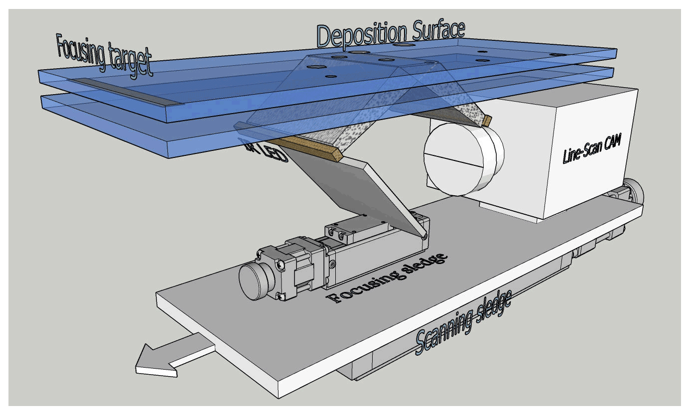
Figure 2ICE-CAMERA basics: the scan sledge moves the image-acquisition line along the deposition surface. The focusing sledge adjusts the focus.
After a complete scan of the DS, the glass is heated and the precipitation sublimated (Sect. 2.7). Once cooled down, the clean SD begins to accumulate new particles. This cycle takes place every hour. After each image acquisition, the MATLAB image processing code is called to process the DS image, and a summary image containing only segmented particles (if present) is stored for post-processing (Sect. 4.1.3). Every particle is also automatically measured through image processing (Sect. 4.1) and classified through machine learning (Sect. 4.2). Individual particle data, along with weather and housekeeping data, are stored in rows in a text file for post-processing and statistical analysis.
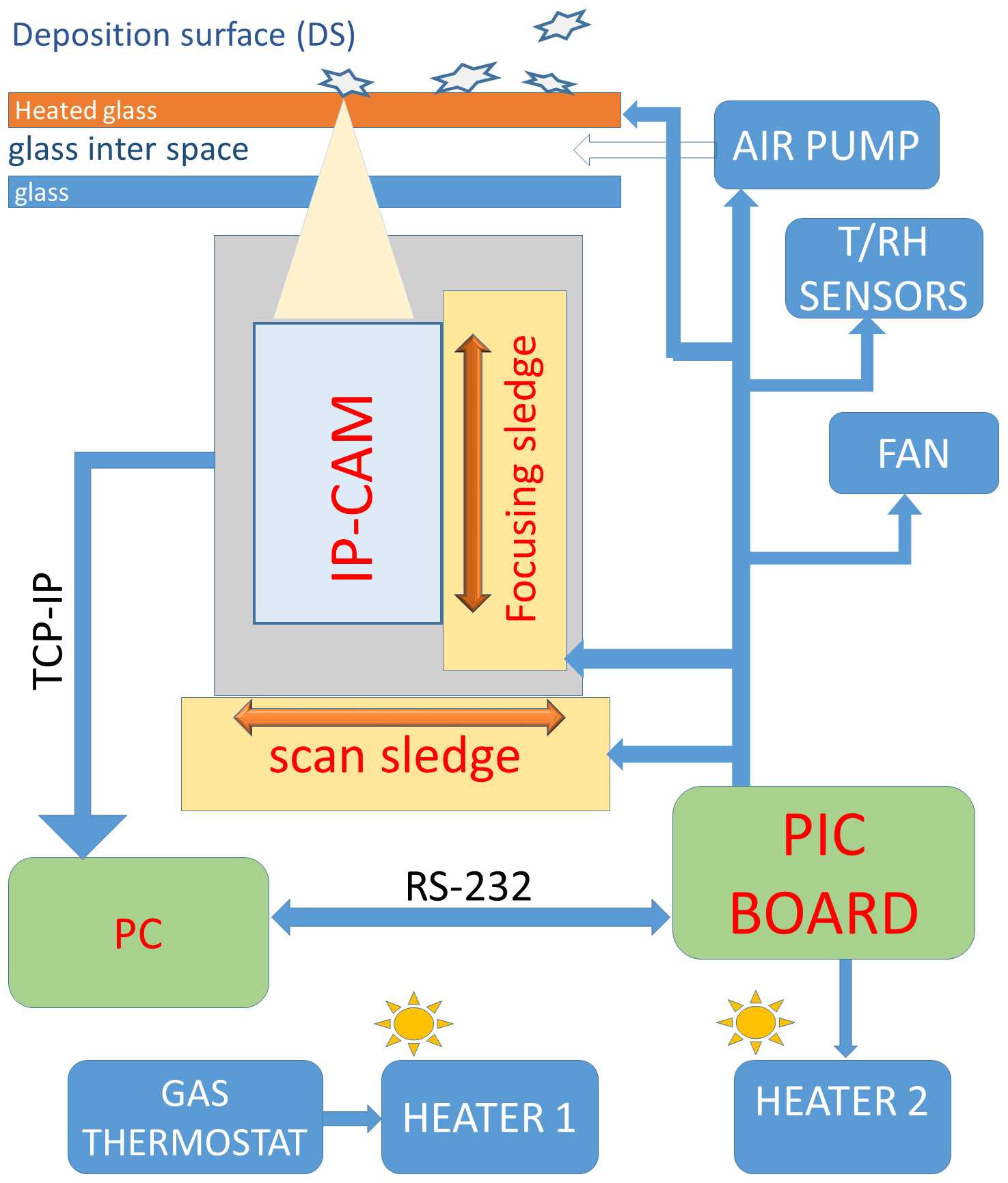
All basic operations of ICE-CAMERA, (with the exception of CAM acquisition) are driven by a custom microprocessor (Microchip PIC) logic board (Fig. 3). The same PIC board reads the housekeeping temperature sensors (attached to the DS and placed inside and outside the instrument), drives the stepper motors of the sledges, and pumps and fans. The PIC board communicates with the main computer (located inside the shelter) through RS232. NI LabVIEW software controls image acquisition, reads maintenance data, and monitors PIC operations along the RS232 line. The line-scan camera communicates with the PC via Gigabit Ethernet.
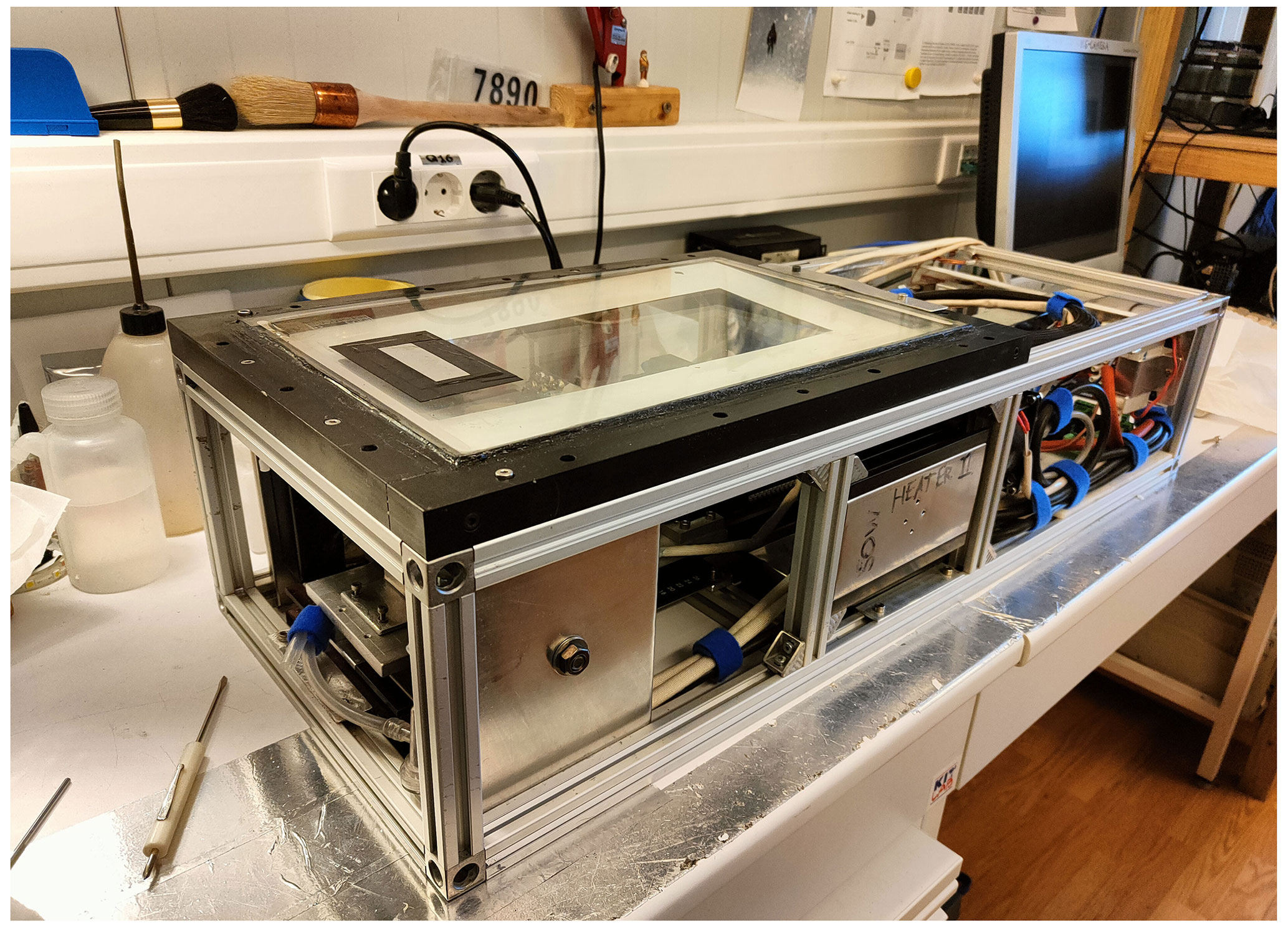
The instrument is placed outdoors, on the roof of the “Physique” shelter, approximately 6 m above the ground. ICE-CAMERA was first installed in Concordia in 2012 but was replaced in 2014 with its improved version, described here. From then on, the instrument works year-round to produce precipitation data every hour. Standard meteorological data are automatically obtained from the local weather station, AWS MILOS 520.
2.2 The line-scan camera
A linear-scanning GigE Vision monochrome camera (Schäfter+Kirchhoff SK7500VTF-XB; 52.5 mm sensor, 7500 pixels, 7×7 µm pixels, 8.2 kHz line frequency), equipped with a 1:1 macro lens (APO-Rodagon D1X, f5.6), is used for the acquisition. The optics were designed by Schäfter+Kirchhoff in order to have a resolution equivalent to the 7 µm pixel size. The 45∘ mirror is used to look upward. The illumination is ensured by 850 nm LEDs. A colour filter (Schott RG715, 800–1000 nm band pass) was used on the CAM lens in order to have a fully solar-blind instrument. The line-scan camera assembly is moved, hourly, by a motorised sledge at a speed of 8 mm s−1 in order to scan the rectangular DS (55×200 mm), located at the centre of the window. The final image is 7500×30 000 pixels, 12 bits, monochrome. A fine calibration of the actual pixel size of the DS image was achieved by scanning a calibrated grid (0.1 mm spacing) placed on the DS. This is necessary, because the effective resolution of the image produced by the moving linear camera along the sledge direction depends on how fast the sledge moves. After the correction of this effect, the image pixel size resulted in 6.97×6.9 µm, which was extremely close to the simulated size of 7×7 µm. From the Nyquist sampling theorem, details less than 14 µm cannot be detected in the image (under optimal focusing conditions). This resolution is enough, for example, for the observation of the hexagonal edges of the smallest plates detected by the instrument.
2.3 The focusing
In working conditions, the focal depth is ±0.5 mm. A preliminary and accurate alignment of the motorised sledge plane to the DS ensures uniformity of focus across the DS at air temperature. A motorised focusing sledge, which moves the bending mirror, allows one to adjust the focus in operating conditions (Fig. 2). As ICE-CAMERA works outdoors at DC, it can experience a broad internal temperature range, from +5 ∘C in summer to −45 ∘C in winter, with quite large temperature gradients across the structure. Thermal expansion and changes in optical refractive indexes result in unpredictable changes in the focal plane. The correction of the focus is thus automatically performed every 6 h by bringing the measuring sledge outside the DS, where a focusing spot (a sandpaper strip) is glued to the window (Fig. 4).
The porous structure of the sandpaper has a length scale on the order of 0.1 mm, comparable with the size of the measured ice particles. While calibrating, the focusing sledge is moved by ±2 mm around the actual position in 0.25 mm steps. Successive images of the sandpaper are taken, and their contrast (defined as the standard deviation of the intensity of the pixels) is measured. After a Gaussian fit of the contrast as a function of defocusing (Fig. 5), the position corresponding to the maximum contrast is obtained, and the mirror sledge is moved into that position. The typical focal spot adjustment between two consecutive calibrations is 0–0.25 mm. The calibration takes approximately 5 min. For this reason, it is not done after each measurement so as to save PC resources for data processing.

Figure 5Typical focus calibration; contrast is calculated in three sectors of the image: centre, left, and right. The contrast throughout the image is also displayed (red). The slight difference in focus (0.2 mm) between the centre of the image and the side wings is a normal lens effect.
2.4 Illumination
Lighting is supplied by two 850 nm LED (TSHG6200) strips. Both arrays illuminate the scan line symmetrically and approximately 45∘ from the optic axis in order to minimise multiple reflections in the double glass and within the camera lens. Infrared illumination was chosen in order to work in solar-blind conditions. This is particularly important, as the linear-scanning camera always looks upward to the sky. The uniformity of lighting along the linear CCD image was tested by taking an image of the same sandpaper used in the focus. The intensity profile along the CCD image was measured, and the intensity of the LEDs was eventually changed to have a final intensity uniformity of less than 15 % across the entire frame.
2.5 The deposition surface (DS)
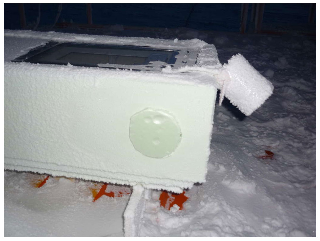
The DS is the external surface of a 10 mm thick, electrically heated glass (E-GLAS, Saint-Gobain). The glass is a sandwich, with an electrically conductive layer pressed between two usual glass sheets. This glass is transparent at 850 nm and can be electrically heated with 45 V ac, 95 W. A second 2 mm thick, optically graded glass sheet (an ordinary flatbed scanner optical glass), placed 13 mm under the DS, makes up with the DS a double glass. This arrangement is necessary in order to keep the DS thermally insulated from the heated interior of the instrument. A thermocouple is attached to the DS, while other thermocouples monitor the double-glass interspace temperatures. A temperature of (at least) 3 ∘C above air temperature is enough to prevent the formation of frost on surfaces in DC in any season, as suggested by the work of Tremblin et al. (2011). In ICE-CAMERA, the temperature of the DS is usually 4 to 5 ∘C above room temperature, which keeps the DS free of frost in all seasons (Fig. 6).
During the sublimation period (Sect. 2.7), ambient air is pumped for 5 min by means of a 3.5 L m−1 miniature pump through the double-glass interspace in order to keep the internal surfaces of the double glass always free of frost. Using inert gases such as argon in the double-glass space for the same purpose proved unsuccessful in Concordia at the extremely low winter temperatures. In order to avoid the eventual accumulation of wind-drifted snow, the DS has no walls or obstacles all around. Furthermore, the instrument is located on the roof of a shelter, almost 6 m above the ground, an altitude where blowing snow is not normally important at Concordia. Libois et al. (2014) identify drifting snow events at Dome C when the 10 m wind speed exceeds 7 m s−1. Assuming a logarithmic wind speed profile between the surface and 10 m and an aerodynamic roughness length value of 1 mm (Vignon et al., 2017), this corresponds to a wind speed threshold value of 5 m s−1 at 6 m above the ground. Winds below this threshold (near the annual average wind speed in DC) are not expected to carry blowing snow to the DS. In addition, blowing snow impacts the flat horizontal and smooth DS at very small angles, with a very limited chance of sticking to it. As a consequence, ice particles collected on the DS can be considered representative of precipitation. In the case of strong winds, not only is the attachment of blowing snow to the DS very low, but the collection of eventual precipitation is also reduced. Since the DS is warmer than air, there is no secondary growth in deposited ice. Instead, the partial sublimation of ice particles before scanning could not be excluded, especially in summer. This topic needs additional field work and will be modelled in Sect. 3.2.
2.6 The thermal control
The temperatures measured by the ICE-CAMERA sensors are continuously transferred to the computer. The NI LabVIEW software controls the internal temperature of ICE-CAMERA, keeping it above −40 ∘C (by driving the 200 W, ventilated air heater “Heater 2” of Fig. 3), and the DS temperature, always keeping it under −5 ∘C (by eventually disabling the “heated glass” of Fig. 3). These conditions are maintained throughout the year during every phase of the measuring cycle. An independent 200 W thermostat (“Heater 1” in Fig. 3) provides emergency temperature control in case of computer or PIC board failure. After a blackout, when the power is restored, a timer is used to heat the inside of the instrument before turning on the electronics. This is important at Concordia to prevent damage to standard electronics with typical operating temperatures of −40 ∘C. In winter, a 40 mm thick Styrofoam coat is added around the instrument for increasing thermal insulation, whereas in summer, a Mylar sunscreen prevents overheating of the instrument and allows the DS to be kept below −5 ∘C on the warmest days (Fig. 1). Additionally, in warm weather, outdoor air is carried inside the box with a tangential fan for better cooling of the instrument.
2.7 Sublimation–deposition cycle
After an entire scan of the DS, electricity is applied to the DS glass to sublimate the particles. The heating rate of the DS depends primarily on the electrical power applied to the glass and its thermal constant (approximately 0.8 W m−1 K−1) and secondarily on the wind speed. An indoor test (Fig. 7) showed a heating of rate of 2.5 ∘C min−1 and a cooling rate of 1 ∘C min−1.

Figure 7Indoor test of DS heating and cooling within a 60 min cycle. For reasons of simplicity, the periods of sublimation and deposition are well separated.
The cooling rate is, at most, only about 50 % of the heating rate. Cooling is passive through heat transfer to ambient air, with a heat transfer coefficient of approximately k=0.024 W m−1 K−1 in still air; k increases with radiation cooling, convection, and wind. During glass heating, heat is quickly transferred to the DS from the electrically heated inner layer, while during cooling, the heat transfer from the DS to the air occurs slowly, with a thermal constant k. This explains the asymmetrical curve of Fig. 7.
Outdoor tests carried out in summer at DC (−30 ∘C air temperature) showed a heating rate of 3 ∘C min−1 in still air, 2.5 ∘C min−1 with 2.5 m s−1 wind speed, and 1.8 ∘C min−1 with 5 m s−1 wind speed. In all cases, the cooling rate was approximately 1.5 ∘C min−1.
An outdoor sublimation test (−30 ∘C air temperature, RH =60 %, wind speed <3 m s−1) performed with snow manually spread on the DS showed that, after applying heating for 10 min (up to a DS temperature of −8 ∘C), the sublimation of the majority of particles (diameter <1000 µm) was complete within 20 min after turning off the heating, with just a few big grains (initial diameter >1000 µm) still present after 30 min.
After these tests, the glass heating period was set at 10 min (the heating is stopped anyway if the DS temperature exceeds −5 ∘C to avoid melting of the ice in summer). At the peak of the sublimation period, the DS was warmer than the air by about dT=20 ∘C (defining dT as the difference between DS and air temperatures). Once the heater is turned off and after a cooling time of approximately 20 min, the DS temperature comes back to being warmer than the air by only 4–5 ∘C. At this point, the “sublimation period” (of approximately 30 min) is considered complete, and ice particles start accumulating again on the DS with no relevant sublimation – i.e. the “deposition period” begins (as sketched in Fig. 7 for the indoor test). At the end of the deposition period, a scan of the DS is carried out for a duration of 1 min. If no ice particles were detected on the previous scan, the DS heater is not applied, and sublimation is not needed. The effective deposition period depends on the temperature, wind, and exposure to the sun in summer. This uncertainty, combined with occasional wind removal and particulate sublimation (Sect. 3.2) during the deposition period, prevents the use of ICE-CAMERA for rigorous quantitative precipitation studies.
DS surface temperature is actually measured by using a small thermocouple. This measurement implies great uncertainties due to the radiant warming of the sensor in summer and the difficult thermal coupling with the glass surface. A non-contact measurement of DS temperature by means of IR sensors would also be ineffective in winter conditions.
3.1 Adhesion of ice particles on the DS
The adhesion of ice crystals to the smooth DS can be attributed to two principal causes: van der Waals and electrostatic forces. Eidevåg et al. (2020) studied the adhesion of dry snow particles after a 90∘ impact to different wall materials (gravity is a minor force in this application, and therefore, their work applies to any wall orientation). They considered models for normal direction, tangential sliding, and tangential rolling that account for the adhesive interaction of spherical ice particles (25–275 µm diameter) and their aggregates. The Johnson–Kendall–Roberts (JKR) model for adhesion was used. Their findings showed that the maximum normal velocity at which spherical ice particles adhere to a glass surface (critical stick velocity) decreases with decreasing particle diameter. Spherical particles of 100 µm would adhere for speeds less than 0.02 m s−1. The numerical method of Eidevåg et al. (2020) has been applied in the present work to compute the critical sticking velocity of spherical ice particles up to 1000 µm diameter. The sedimentation velocity of ice crystals up to 1000 µm was also calculated using the formulation of Böhm (1989) for DC conditions (Tair ∘C, air density =1.03 kg m−3, dynamic viscosity Pa s). Particles impacting on the DS with a sedimentation velocity lower than the critical sticking velocity are immediately captured with 100 % efficiency by van der Waals forces. The simulation shows that only spherical particles smaller than 50 µm in diameter fall on the DS with a speed smaller than the critical stick velocity and thus stick immediately. This result does not change with the different forms of particles, as for these sizes, the speed of sedimentation is close to that of Stokes. Particles above 50 µm in diameter have an excess of kinetic energy to bind immediately and effectively on the DS. However, the impact surface (DS) is horizontal, so the excess kinetic energy is rapidly dissipated in one or more vertical rebounds until the critical sticking velocity is achieved (Chokshi et al., 1993). So, the adherence of ice crystals to the DS could also be explained by the forces of van der Waals alone. Ryzhkin and Petrenko (1997) showed that static charges, naturally transported by ice crystals, increase adhesion. The electrostatic interaction between the ice and the surface is significantly stronger than the van der Waals forces at distances greater than the intermolecular forces. Electrostatic forces are therefore expected to significantly improve the adhesion of large ice particles to the DS.
Once attached to the DS, the weak winds generally observed at DC cannot detach the particles from the DS. Particulates are protected by the boundary layer (BL) that forms on the DS. The 99 % thickness of the laminar BL (Blasius solution) at the centre of the DS (0.15 m distance from the glass edge) is expected to be 7 mm at −50 ∘C, with a wind speed of 1 m s−1, decreasing to 2 mm at 10 m s−1. As a result, the particles deposited on the DS are protected against the wind.
3.2 Sublimation of ice particles
The DS is always warmer than the surrounding air. This is necessary to eliminate hoar, enabling the device to be used in all DC conditions. The undesirable effect is the accelerated natural sublimation of deposited particles. A wide range of experimental and theoretical research efforts has characterised the effects of temperature and super-saturation on ice crystal growth rates and morphology under conditions relevant to atmospheric processes (for example: Lamb and Hobbs, 1971; Libbrecht, 2005, 2017). The wide variety of ice crystals found in nature has sparked an interest. Sublimation was sometimes regarded either as the opposite process or as a less intriguing process and was thus less visited in laboratory studies. Nelson (1988) sublimated numerous 100 µm diameter plate crystals (0.1 ∘C ∘C, 0.05 % to 5 % sub-saturation), showing that the crystals first lost sharp edges and finally evolved into spheroidal particles and that the aspect ratio remained almost constant. The sublimation rates were accurately predicted by the diffusion equation with the surface vapour density at the equilibrium value for a uniform surface temperature. The sublimating crystal reaches a self-preserving shape that is one of the shape-preserving solutions of the diffusion equation. Ham (1959) showed that ellipsoids and thus spheroids preserve shape during growth and sublimation if the grain surface has a uniform temperature. Jambon-Puillet et al. (2018) also showed experimentally and theoretically that sublimation first smooths out regions of sharp curvature, leading to an ellipsoid. The second stage is the sublimation of the self-preserved ellipsoid shape. The entire process may be modelled as a vapour diffusion problem, mathematically equivalent to the resolution of the electrical potential around a charged conductor. Using this analogy, they provided a mathematical method for simulating the sublimation of the ice particle. The sublimation of the ellipsoid turned out to be mathematically simple, and their method was adopted in this work to simulate numerically the second stage of sublimation of ICE-CAMERA particles.
Monodispersed oblate spheroids with an aspect ratio (AR) of 5, in thermal equilibrium with the DS, were assumed in the simulations as a surrogate for ice plates. The two major spheroid axes coincide with the “diameter” of the oblate spheroid, D. In the model, D, DS temperature, air temperature, and relative humidity with respect to ice (RHair) can be changed. The sublimation time required for full sublimation of a spheroidal ice particle was computed. As sublimation accelerates when the particle is going to vanish, the time necessary for the complete sublimation is only slightly larger than the time necessary to reduce the particle to the minimum particle size (D=60 µm) accepted by ICE-CAMERA image processing. The simulations assume that the preliminary sublimation of the high-curvature parts of the particle (sharp edges, corners, surface irregularities) was already completed so that the calculated time of sublimation must be considered as a lower limit for real-world crystals and probably almost one half of the overall duration of sublimation (Jambon-Puillet et al., 2018). Simulations also assume the thermal equilibrium between the particle and DS, a condition which is not necessarily satisfied on the thermally insulating glass surface of the DS. Figure 8a shows the total sublimation time with the ∘C. The humidity resulted to be irrelevant in this case, and only results for 70 % RHair are shown. Results show that at −30 ∘C air temperature (summer conditions in DC), complete sublimation can occur within a few minutes after attaining the DS sublimation temperature for all particle sizes up to 1 mm. At lower air temperatures, the sublimation time increases: at −70 ∘C (winter temperature in DC), particles smaller than 100 µm in diameter still disappear within 10 min, while larger particles can survive along the sublimation period. Simulations showed that, at −70 ∘C, dT should be increased to dT=60 ∘C in order to ensure the complete sublimation of ice particles up to 1 mm diameter during the sublimation period. This is actually not possible with the electrically heated glass adopted but could probably be achieved by microwave heating.
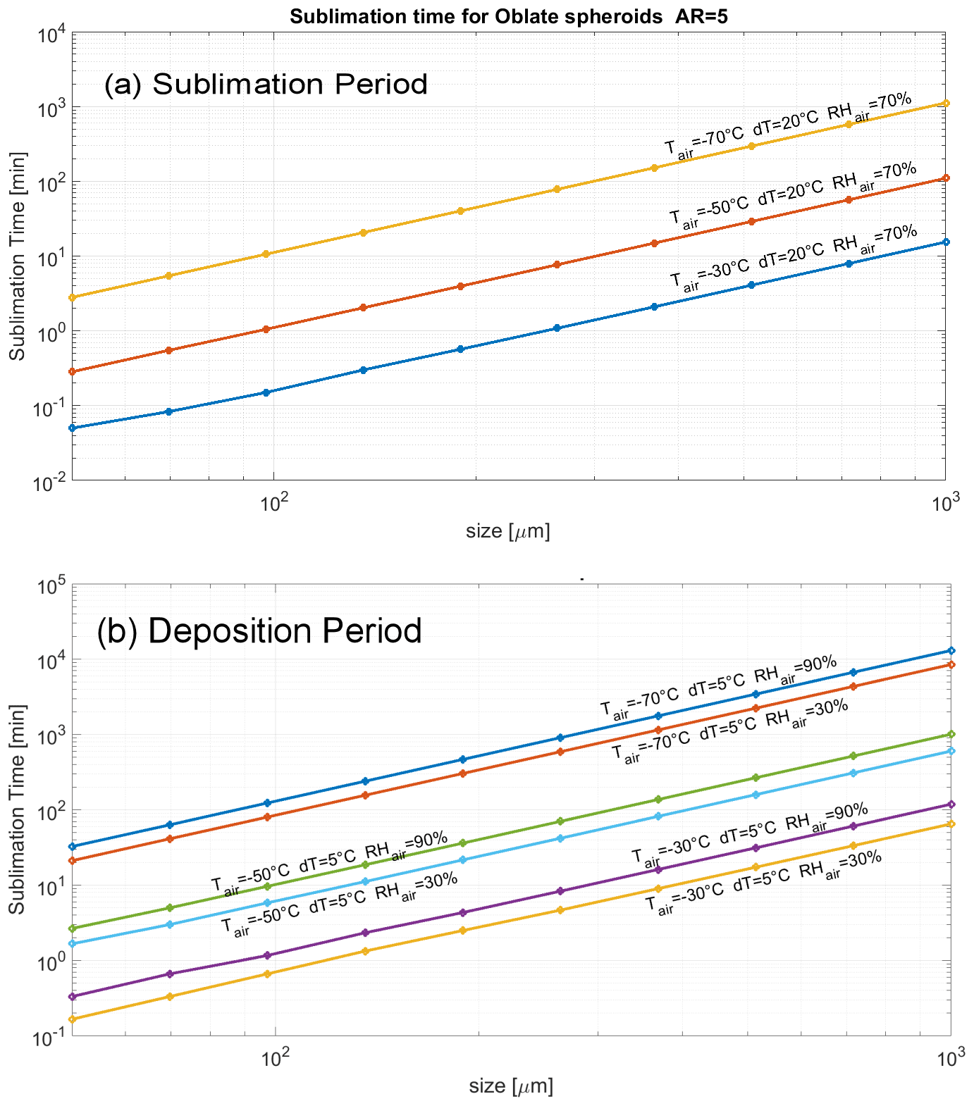
Figure 8Sublimation time of monodisperse oblate spheroids at varying air temperatures, with (a) dT=20 ∘C (sublimation period) and (b) dT=5 ∘C (deposition period).
After the sublimation period, most of the particles previously collected on the DS are sublimated, and a new deposition period begins. Even during this period, sublimation still acts on ice particles, albeit slowly. Figure 8b shows the sublimation time expected for monodisperse spheroids during the deposition period. The DS was considered 5 ∘C hotter than air. As shown, during the deposition period, the relative humidity of air also plays a role, even if secondarily. In summer ( ∘C), sublimation can take less than a minute for particles smaller than 100 µm and 10 min for 300 µm particles. During winter ( ∘C), all particles are expected to survive through the deposition period. As a rule of thumb, simulation showed that working with ∘C resulted in an increase of the rate of sublimation by a factor 2–3 compared with a DS in thermal equilibrium with ambient air (dT=0) for the whole range of air temperatures and RHair shown in Fig. 8b.
Results of Fig. 8b show that the effective lower limit of ICE-CAMERA particle detection is not limited solely to the resolution of the optical system and/or image processing software. In summer, particles smaller than 100 µm may be decimated during deposition, unless they fall just before scanning. Such small particles dominate diamond dust events. As a result, ICE-CAMERA, during the summer period, is best suited to the study of cloud precipitation. Nevertheless, visual screening of ICE-CAMERA images showed only a limited number of small particles revealing signs of partial sublimation, such as rounded corners, smooth edges, or a spheroidal appearance. Some small plates (observed mainly in winter, when sublimation during the deposition period is very slow) showed smoothed corners, but it is not clear if this was induced by sublimation or if it is a natural feature of these ice grains. Also, even in summer, small DD particles such as plates (with no signs of edge smoothing) were normally observed (Sect. 5.2). It is probable that most particles (other than, probably, pristine plates) never achieve thermal equilibrium with the DS glass and that the results of Fig. 8 should be considered as the worst case. Also, the sublimation of the high-curvature parts of the particle prior to assuming the spheroidal form (Jambon-Puillet et al., 2018) could take much more time than the sublimation time calculated here for the spheroid. A series of consecutive DS scans at fixed air temperatures is needed to measure the effective sublimation rate of small particles in deposition conditions ( ∘C).
When a polydisperse particle population is deposited on the DS instead of monodisperse particles, a more complicated sublimation picture arises, because small spheroidal particles, shrinking, are continuously replaced in the size distribution by sublimating, initially bigger ones. An initial uniform particle size distribution (PSD) of the oblate spheroids (AR =5) was assumed, with diameters between D=1 and 2000 µm for the simulations. The evolution over time (1 s resolution) of the PSD was calculated (Fig. 9) in terms of particle survival (the ratio between the actual number of particles in a certain size bin and the initial number in the same bin). No vapour competition between ice particles was taken into consideration in the simulations. Results are similar to those of monodisperse particles (Fig. 8), with a slightly longer time of sublimation for polydisperse particles compared to monodisperse particles of the same size. Results for an air temperature of −70 ∘C confirm that most particles larger than 500 µm survive for more than 30 min throughout the DS sublimation period (dT=20 ∘C). This means that sublimating by heating the glass is quite inefficient for large particles in winter. During the deposition period, at −70 ∘C, losses for sublimation are scarce and limited to particles smaller than 200 µm. Consequently, double counting of the same particle (D>500 µm) is possible in two consecutive ICE-CAMERA scans in the cold DC winter. At −30 ∘C air temperature (summer), the heating of the DS with dT=20 ∘C leads to the sublimation of most particles up to 2 mm diameter within 5 min. On the other side, during the deposition period, particles smaller than 500 µm can undergo sublimation over a period of just 10 min in summer, thus limiting the effective period of deposition before a scan. As with monodisperse particles, this introduces bias in the summer, because many small particles (typical of DD) can be removed before they are measured.

Figure 9Evolution of an originally uniform PSD of ice spheroids (D= 0–2000 µm, AR =5) under different atmospheric conditions (RHair is a secondary factor affecting the results, shown here for RH =70 %). (a, c) Sublimation period; (b, d) deposition period. (a, b) Winter, (c, d) summer.
Even if these results could be disappointing for interpreting ICE-CAMERA data, the same problems affect the actual method of observing precipitation in DC: collecting and observing (every 24 h) the ice particles deposited on flat surfaces (“benches”) is affected by the same problem as collecting particles on the ICE-CAMERA DS with dT=0. Fluctuations in relative humidity over 24 h result in sublimation and regrowth of particles on the “benches” in an almost unpredictable manner. Figure 10 shows the expected sublimation time for particles (with the same PSD of Fig. 9) placed on “benches” (or ICE-CAMERA DS) in equilibrium with air (dT=0) for extreme, sub-saturated conditions: winter ∘C (RHair=30 % and 99 %), and summer ∘C (RHair=30 % and 99 %). The PSD evolution is computed with a resolution of 1 s for a total period of 6 h. The results show that sublimation also works in winter and with almost saturated air (99 % RHair), leading to a complete loss of small particles (D<200 µm) in a few hours. In summer conditions and 30 % RHair, sublimation happens much more quickly, with the disappearance of all particles up to 2000 µm in 30 min. With RHair=99 %, sublimation removes all particles in just a few hours in summer. In the presence of wind and dry air, the sublimation rate could even increase, as observed by Grazioli et al. (2017b) in coastal areas. These simulations all refer to sub-saturated conditions: in the case of a “bench” in thermal equilibrium with super-saturated air, hoar form on the surface, with a possible confusion with precipitation.
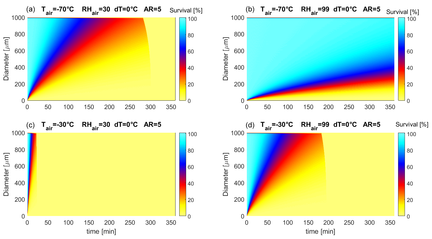
Figure 10Evolution of an originally uniform PSD of ice spheroids (D= 0–2000 µm, AR =5) under different atmospheric conditions. The DS (or “bench”) is in thermal equilibrium with air (dT=0). (a, b) Winter, (c, d) summer.
4.1 Image processing
ICE-CAMERA is not just designed to take photographs of ice particles but also to provide automatic morphometry and classifications of polar precipitation. This was accomplished through the use of image processing and machine learning techniques. The process is divided into two parts: segmentation and measuring, and classification of ice crystals.
4.1.1 Image segmentation and measurement of ice particles
After acquisition, using MATLAB software, the raw ICE-CAMERA scans are segmented in order to isolate all detected particles. The process follows the workflow of Fig. 11. Refer to Pratt (2007) for image-processing nomenclature, to Walton (1948) for Feret measurement, and to Russ and Brent Neal (2017) for the nomenclature of standard shape parameters such as eccentricity, Euler number, circularity, roundness, solidity, compactness, form factor, and number of skeletal branches. The normalised central moments f1…f7 were also computed, as described by Hu (1962). The aspect ratio (AR) is defined as Feret's length/Feret's width. The Feret-box surface-equivalent diameter (Df) is defined as the diameter of the circle having the same area as the Feret bounding box, while the surface-equivalent diameter (Ds) is defined as the diameter of the circle having the same area as the segmented ice grain. The main steps of Fig. 11 are visually summarised in Fig. 12 for a rimed, columnar particle.
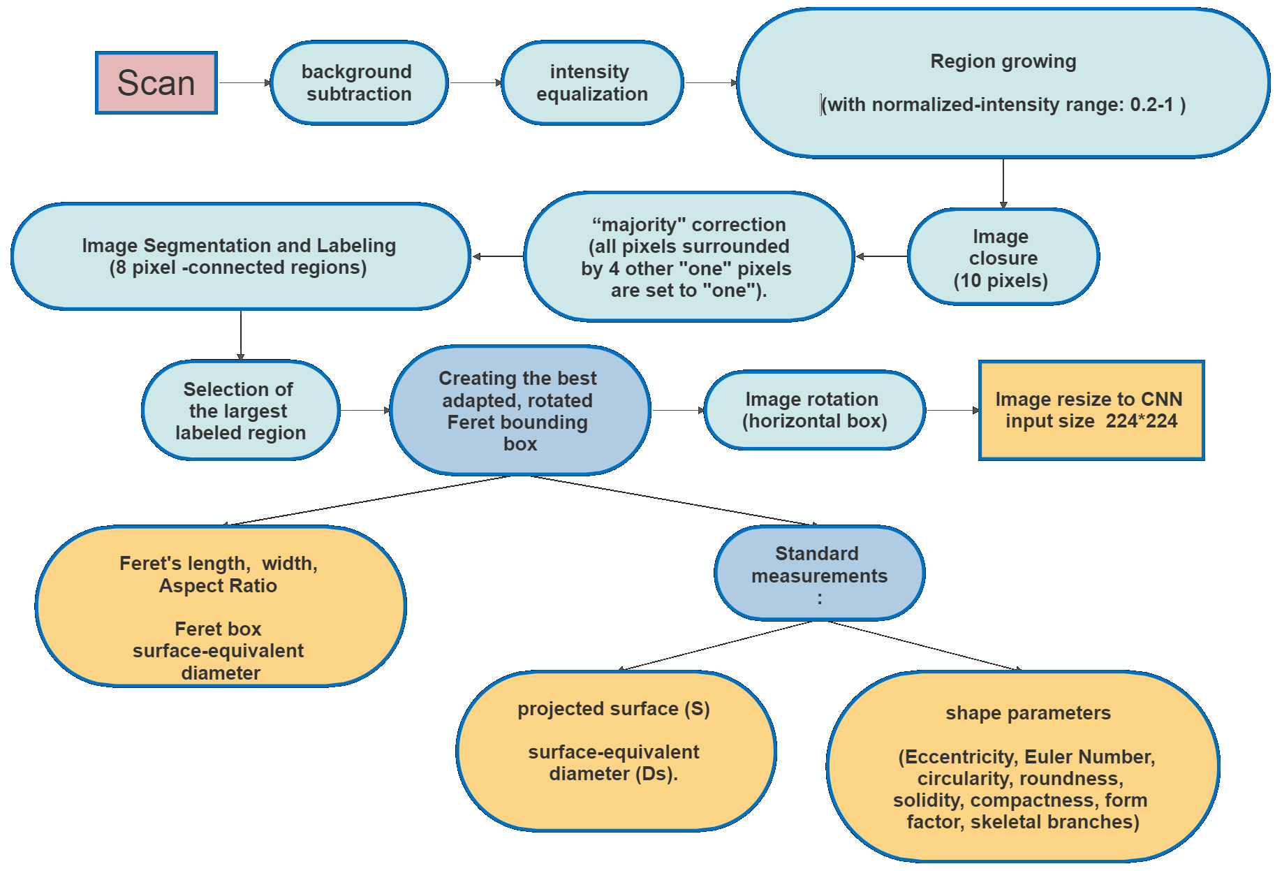
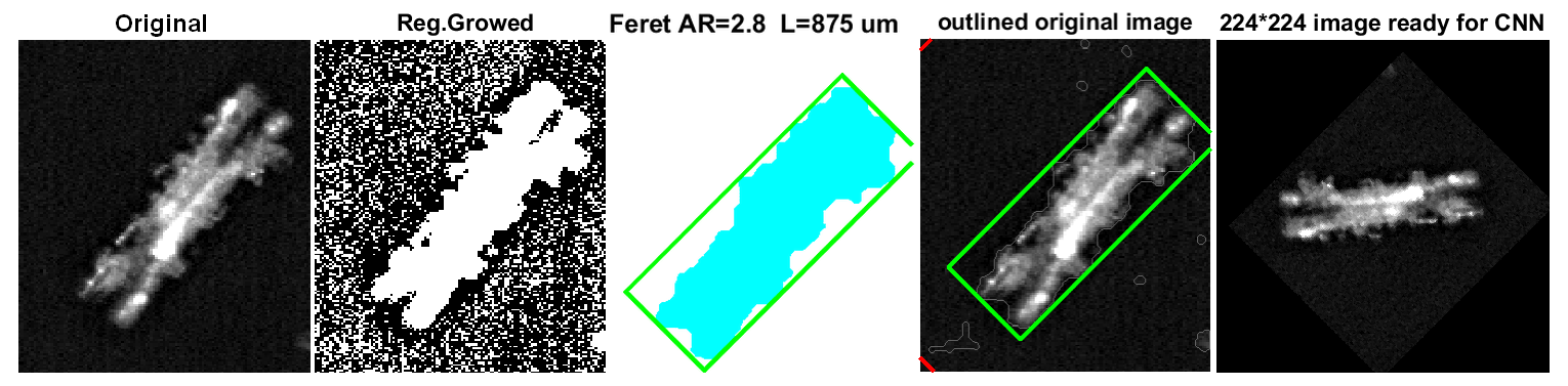
Figure 12The original image (in this case, a rimed column) is segmented using “region growing”. The projected particle area (clear blue) is calculated. The bounding box is determined (green) and the Feret length and width measured. The image is finally rotated to have the mayor axis horizontal, re-scaled, and resized to the CNN input size.
4.1.2 Summary image of detected particles
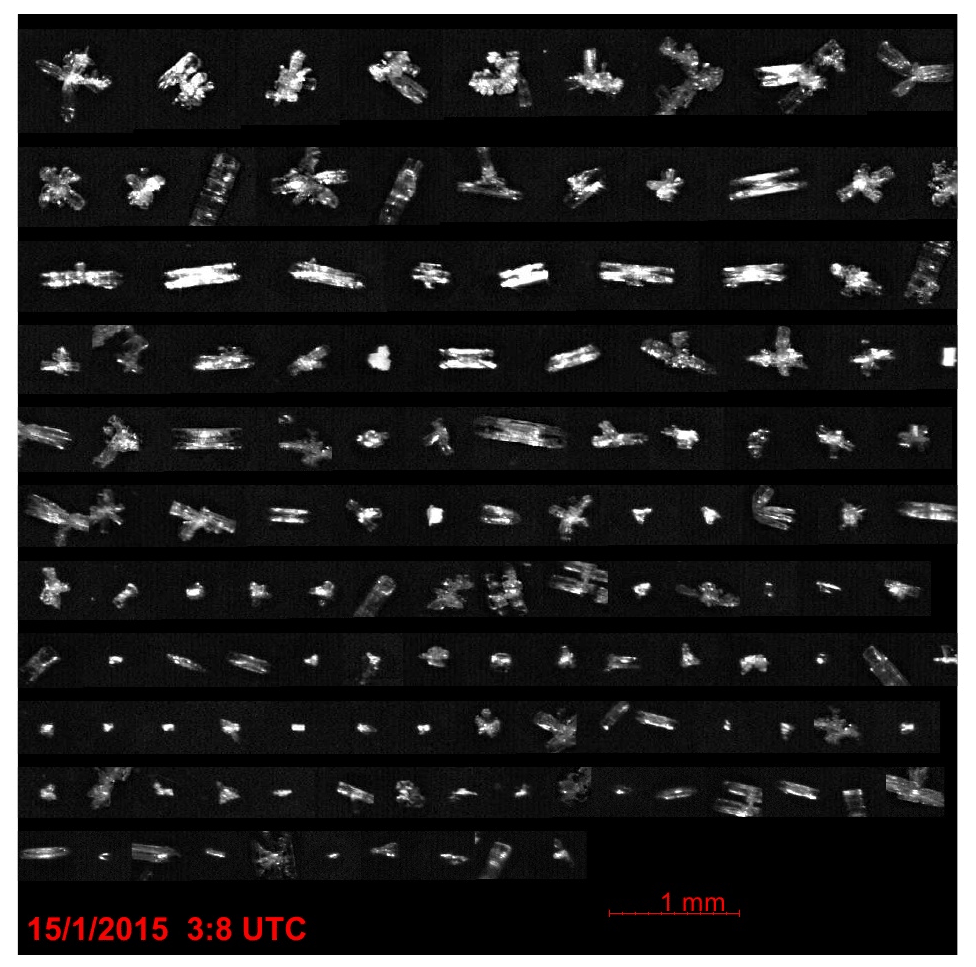
The bounding boxes of all individual ice particles detected in a scan are sorted by Feret length and are reassembled in a summary image that collects all segmented particles (Fig. 13). Each particle is also associated with a numerical record containing the coordinates of its bounding rectangle on the summary image, shape parameters, time of acquisition, and local weather data. In this way, the re-analysis of the summary image is possible instead of re-processing the original, large image. The original image is ultimately removed.
4.1.3 Limitations and uncertainties in detecting and sizing ice particles
-
The total number of particles measured is actually limited to 2000 per scan, as a result of MATLAB memory limitations. Extra particles are not treated.
-
Particles below 3600 µm2 in bounding-box surface (equivalent to approximately 60 µm in diameter for a spherical particle) are not preprocessed (smaller particles could be detected, but most have a seemingly circular shape due to low pixelation or poor focus).
-
The segmentation becomes difficult when overlapping particles or aggregates of particles are present. In such situations, double counting of the same particle may occur in up to 12 % of a scan in the presence of an intense precipitation event. The same particles can, in fact, fall inside different segmented areas of the image because of the lack of defined boundaries between particles on the original image. The process of “region growing”, which leads to segmented particles, can actually start independently from several bright (“seed”) regions located in different parts of the image of the overlapping particles. The “region-growing” processes can then propagate through the overlapping particles, leading to several “copies” of the same, segmented image. This unwanted effect could be prevented by looking for similar copies of the same segmented image, but this method was not implemented at DC due to limited PC resources. Overlapping particles are normally classed by the CNN algorithm as “clusters”. A few occasional arrangements of three or more overlapping columns are sometimes mistaken for single plates. The Feret measurement of these particles is meaningless. At DC, this situation occurs only after heavy cloud precipitation, which is a relatively rare event.
-
Multiple counts of the same particle also occur for non-overlapping particles when multiple bright spots exist within the same particle. As in (3), the region-growing process can start independently from several “hotspots”, leading to false copies of the same segmented particle. This effect could potentially be avoided by comparing segmented images and deleting copies, but this method was not implemented at DC.
-
Particles close each other in the original image could be segmented into a single particle by region growing and could thus be misclassified.
-
In the case of defocused images, the particle shapes are all close to a fuzzy, round, or elliptical shape, which can cause a misclassification into irregular particles, spheroidal particles, or plates. ICE-CAMERA images dominated by these types of particles are normally eliminated during a preliminary manual screening. Also, a few big particles in summer resulted in being rounded by partial sublimation. A few images containing only rounded or “spheroidal” particles that were 500 µm or more in diameter were collected during the warmest part of summer and were manually discarded before the statistical data analysis.
-
Needles and hexagonal plates (typically small, see Fig. 23) may be very bright in ICE-CAMERA images due to enhanced light diffusion at preferred angles. For the same reason, hollow columns sometimes have a shiny spot in the middle. In the case of needles, this effect can reduce the apparent aspect ratio, as the width is apparently increased by the scattered light saturating the camera. For plates, the bright specular reflection sometimes blurs the polygonal contour, especially in the case of small plates.
4.2 Automated classification of ice particles
An initial attempt at automatic classification of ICE-CAMERA segmented images was made in 2014 using shape factors. This kind of technique has also been used by others (e.g. Lindqvist et al., 2012) for attempting the classification of ice particles. In the case of ICE-CAMERA, this approach resulted in being extremely unreliable. A much more promising approach was offered after 2015 by the rapid development of transfer learning and convolutional neural networks (CNN) (LeCun et al., 2015; Schmidhuber, 2014). Xiao et al. (2019) successfully applied deep transfer learning to ice particle images obtained with airborne Cloud Particle Imagers (CPI). The CNN approach has added much value to ICE-CAMERA, because a reliable classification of ice particles into simplified classes became possible. The CNN used for the ICE-CAMERA particle classification is “GoogleNet” (Szegedy et al., 2015), a variant of the Inception network, a deep convolutional neuronal network developed by Google scientists. GoogleNet is a type of convolutional neural network based on the Inception architecture. It utilises Inception modules, which allow the network to choose between multiple convolutional filter sizes in each block. The GoogleNet architecture consists of 22 layers (27 layers including pooling layers), and part of these layers are a total of 9 inception modules. In this work, GoogleNet was used in the MATLAB R2020b environment. The GoogleNet CNN, pretrained on the ImageNet dataset (Deng et al., 2009), was used, with its final, fully connected layer changed to size 14. The input layer of the GoogleNet architecture requires images of size 224×224.
4.2.1 The CNN classification classes
Low temperatures and humidity on the high Antarctic plateau reduce the diversity of ice particle shapes. This is observed on the field at DC, at the South Pole station (Lawson et al., 2006), and is suggested by review works such as Bailey and Hallett (2009).
Following an initial survey of the ICE-CAMERA image database, a set of 14 types of particles was selected, as shown in Fig. 14. When choosing the 14 classes, I assumed that shapes easily recognisable by a human operator could also be easily recognisable by a CNN.
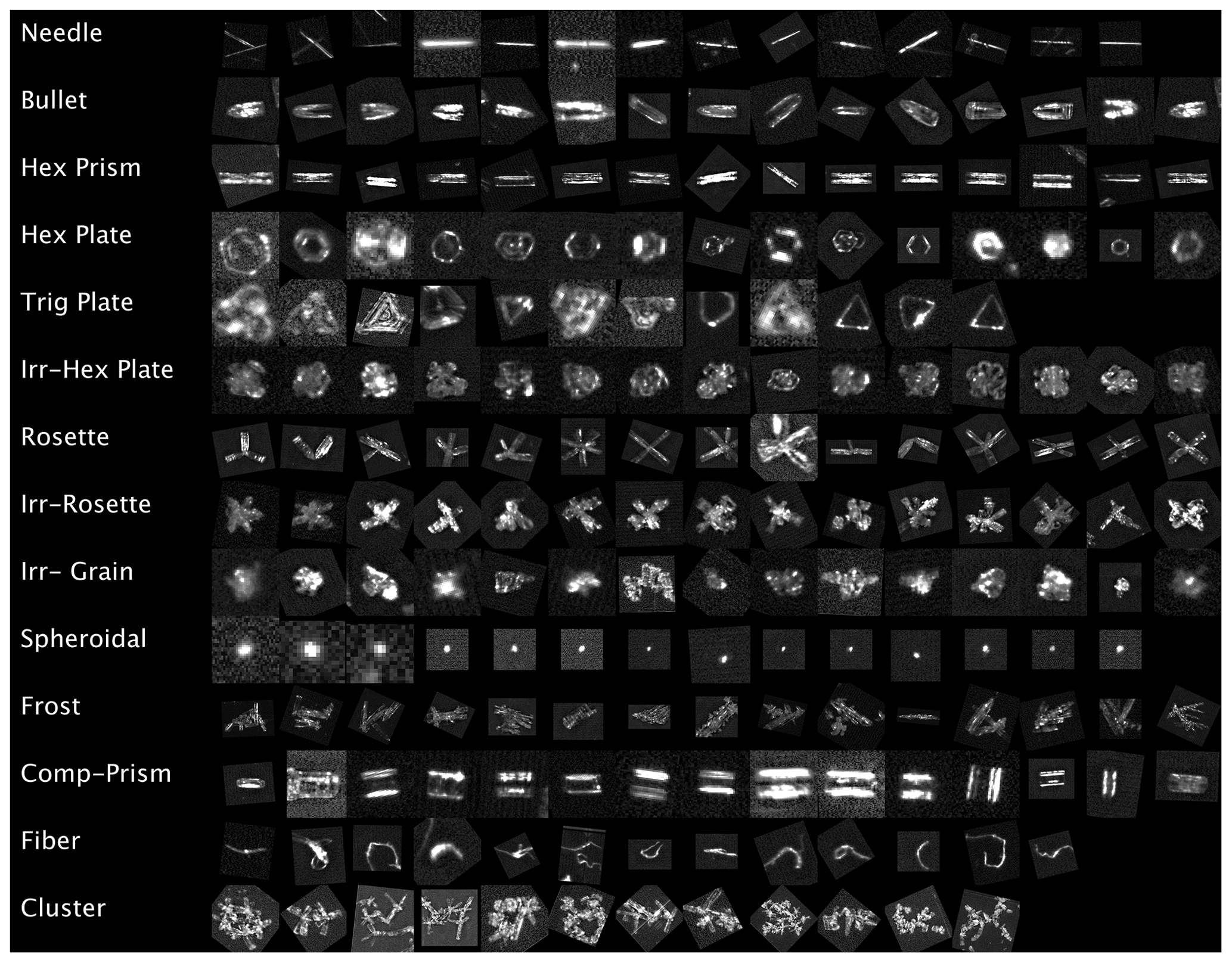
Figure 14A sample of ICE-CAMERA images of the 14 classes of ice particles used to train the CNN.
In the following scheme, I tried to fit the classes chosen for ICE-CAMERA with the classification scheme of the ice particles of Kikuchi et al. (2013), an updated version of the original classification of Magono and Lee (1966):
-
needles: covering the classes C1a, C1b, and C3d (Kikuchi et al., 2013);
-
bullets: covering the C4b–C4c classes;
-
columns: columns covering classes C2a, R2b, C3a, and C3b;
-
hexagonal plates: covering classes P1a, P1b, P1c, P4f, G2a, G3a, CP3f, and CP3d;
-
trigonal plates: covering the class G2b;
-
irregular plates: plate-like particles with irregularities, riming, overgrowing plates, etc. but keeping a basic hexagonal shape, covering P6a, P6b, P7a, CP6d, R1b, R2b, R2c, R3a, and G4b;
-
rosettes: bullet rosettes or column rosettes, with a minimum of two branches, covering C2c, C3e, C4d;
-
irregular rosettes: rosettes with irregularities and riming but preserving the typical stellar outline of rosettes, covering classes P7a, P7b, CP2d, CP4c, CP5a, CP6e, CP6f, CP6g, and R1d;
-
irregular grains: covering CP3e, CP5a, CP6d, G4c, G4a, I3a, I2a, I1a, H1a, and H1b.
-
spheroidal: particles with spheroidal or spherical appearance, covering H1a and H1c; large particles with D>600 µm, detected as “spheroidal” in DC, are usually artefacts caused by defocused images and are not considered in the statistical analysis;
-
compact columns: short columns covering classes G1a and C3a;
-
clusters of particles: covering A1a, A3a, H2a, H1b, P8b, CP3e, CP5a, and CP6h;
-
frost: frost formed on the DS CP7, CP8, and CP9;
-
fibres: non-volatile fibrous material (from local human activities, Styrofoam particles, textile particles, dust, etc.).
The last two classes are not considered in the statistical analysis of ICE-CAMERA data: they are just used to detect occasional frost formed on the DS in case of super-saturation and man-made, non-evaporable (thus persisting on the DS) materials. Uncommon ice particle typologies present at Concordia were not considered in the present work. Trigonal plates have been included, although they are rare, simply because they are seemingly easy to detect with CNN.
4.2.2 The training dataset
For the training of a first CNN, a set of 5500 ICE-CAMERA segmented images of single particles, sampled randomly from the 2014–2017 ICE-CAMERA database, have been manually sorted into 14 image data stores corresponding to the 14 classes. Fourteen of the computer keyboard keys were marked with the symbols of the 14 classes in order to expedite the manual classification of the initial training dataset. These images were used for a first CNN training; 10 % of the images were dedicated to validation, 10 % to testing, and the remaining 80 % to training. The first CNN was used for the classification of the ICE-CAMERA dataset for the years 2014–2017. In addition to the classification, the individual crystal images were also sorted into and stored in 14 folders according to the CNN classification. Selected images from these folders were manually reclassified into all 14 classes (when misclassified by CNN) and added to a second CNN training dataset. Additionally, misclassified images were re-labelled and used in the training dataset for the new CNN. In this way, a potential positive bias of the confusion matrices due to the exclusion of misclassified images in the new training dataset was avoided. In the selection of the new training images, care was taken to ensure a balanced number of training images in the 14 classes. The updated image dataset was finally divided into validation (10 %), test (10 %), and training (80 %) datasets for training a second CNN. This process was repeated three times to expand the training database and thus to improve the overall precision of the CNN classifier.
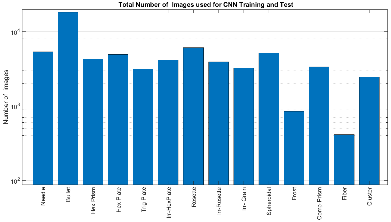
Figure 15 shows the final number of training and test images selected for each class. The total number of images used for the training was 81 800. Trigonal plates were rare, and their number in the training dataset was thus artificially augmented by duplicating the training images in order to avoid their absence in the small (64-images) training mini-batches.
4.2.3 CNN training details
To meet Google's input requirements, all images of single particles were resized to 224×224 pixels. In the training process, “data augmentation” was applied to the original dataset. Artificially “augmenting” the image dataset has been shown to be effective in CNN training (Shorten and Khoshgoftaar, 2019). Images inside each mini-batch are automatically and randomly “augmented” in order to reduce CNN overfitting. The following transformations were used in augmentation:
-
X, Y reflection
-
random X, Y translations ±30 pixels
-
random scaling 80 %–120 %
-
Other changes, such as rotation, have not been introduced, since the ICE-CAMERA images to be classified are typically oriented horizontally by the image processing procedure (e.g. Fig. 13)
The following learning options were utilised in GoogleNet training:
-
solver: stochastic gradient descent with momentum (SGDM)
-
activation: softmax
-
number of epochs =5
-
learn rate =0.001
-
batch size =64
-
L2 weight regularisation factor =0.005
-
validation frequency = every 30 iterations
-
shuffle of the dataset at every epoch
The evolution of the CNN training in terms of accuracy and losses is presented in Fig. 16. The validation line closely tracks the training line, showing the absence of overfitting.

4.2.4 Testing the CNN classifier
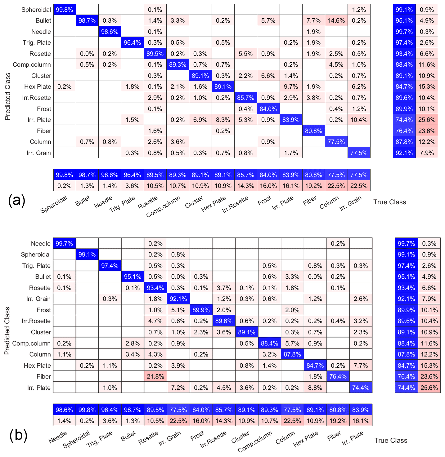
CNN's performance test results are summarised in confusing matrix graphs like Fig. 17a. Each row corresponds to a predicted class (output class), and each column corresponds to a true class (target class). Diagonal cells refer to correctly classified observations. Off-diagonal cells are improperly classified observations (red colour markings increasing misclassification). The column on the far right of the plot shows the percentages of all the examples predicted to belong to each class that are correctly and incorrectly classified (positive predictive value and false discovery rates, respectively). The row at the bottom of the plot shows the percentages of all the examples belonging to each class that are correctly and incorrectly classified (true positive rate and false negative rate, respectively).
4.2.5 Accuracy of the classifier
In the column-normalised summary (Fig. 17a), the percentages along the ith column show the probability (P) of a “true” particle in class ith being classified in each of the 14 output classes.
Reading the columns of Fig. 17a from left to right, the accuracy of the CNN in properly classifying a particle belonging to the ith true class (bottom row) can be assessed. The results are summarised below:
-
There is good accuracy (P>90 %) in identifying needles, spheroidal, bullets, trigonal plates.
-
Compact columns are misclassified into columns (3 % of the time) and bullets (3 % of the time).
-
Hexagonal and irregular plates are confused approximately 10 % of the time; this is expected, since the edges of the plates (usually small) are sometimes blurred in the image.
-
Irregular rosettes are misclassified in 5 % of cases as pristine rosettes and in 5 % of cases as irregular plates.
-
Irregular plates are confused with hexagonal plates 10 % of the time.
-
Irregular grains are sometimes mistaken for irregular plates (10 %) and hex plates (6 %).
-
Columns are misclassified as bullets 15 % of the time.
The three-dimensional structure of the ice particles is lost in the ICE-CAMERA images so that some thick ice forms such as C4a, P1b, G3b, CP1a(Kikuchi et al., 2013), if any, are likely to be misclassified by this CNN.
A different view to read the CNN test is the row-normalised summary of the confusion matrix (Fig. 17b). Percentages along the ith row now show the probability for a particle classified into the ith class to effectively belong to each of the 14 true classes. Reading the rows of Fig. 17b from top to bottom, the results are as follows:
-
Particles classified as needles, spheroidal, trigonal plates, bullets, pristine rosettes, and irregular grains effectively (P>90 %) belong to their class.
-
Particles classified as irregular rosettes have a 5 % chance of being regular rosettes.
-
Particles classified as compact columns have a 6 % chance of being columns.
-
Particles classified as columns have a 4 % chance of being a two-branch rosette and 3 % of being bullets or compact columns.
-
Particles classified as pristine plates have a 4 % chance of being irregular grains.
-
Particles classified as irregular plates have a 7 % chance of being irregular grains, a 9 % chance of being hex. plates, and 5 % chance of being irregular rosettes
5.1 Overview of ICE-CAMERA dataset
From January 2014 to December 2021, ICE-CAMERA had segmented a total of 11 007 543 particles. This gross count includes particulates successively rejected for the statistical analysis. Some whole scans were eventually ignored because of poor focus, sledge motor failures, or the presence of layers of snow or frost. Individual particles were omitted from the analysis due to their small size or defocus. The distribution of the number of particles observed during the months is shown on Fig. 18a. The number of scans per month is shown in Fig. 18b. Under optimal conditions, one scan per hour is planned, with a typical total of 740 scans per month. Some months, problems with ICE-CAMERA focusing or processing software resulted in the small number of scans or particles observed. In most other cases, scans were not recorded when fewer than 10 particles were detected on the DS.
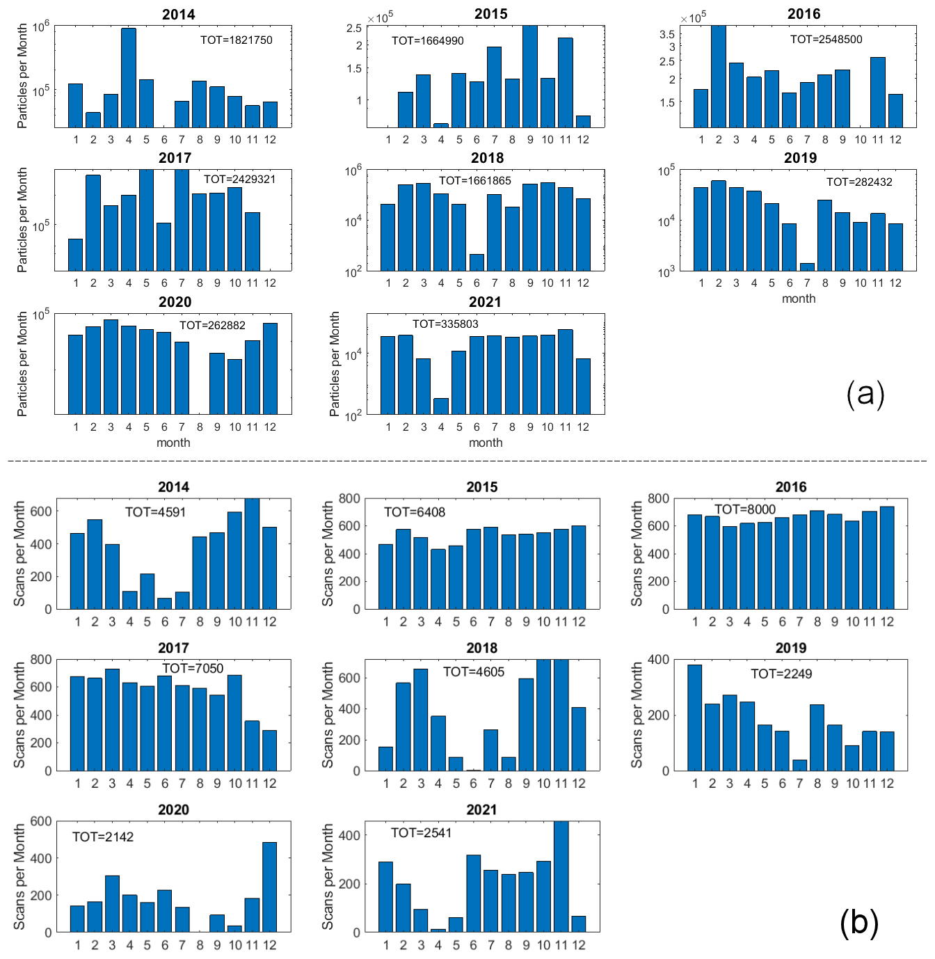
Figure 18Statistics per month for the years 2014 to 2021. (a) Ice particle counts per month (total counts per year are also reported). (b) Number of scans per month (total number per year is also reported).
The number of particles per scan (NpS) is a rough indicator of the intensity of the collected precipitation, but it could be affected by sublimation, because in conditions of “warm” air, the smallest particles could disappear from the DS before being detected (Sect. 3.2). Figure 19a shows the NpS in relation to the air temperature for the whole period 2014–2021 in box and whisker format. On each box, the middle mark indicates the median, and the lower and upper edges indicate the 25th and 75th percentiles, respectively. The lower and upper whiskers indicate an interquartile below the 25th percentile and an interquartile above the 75th percentile.
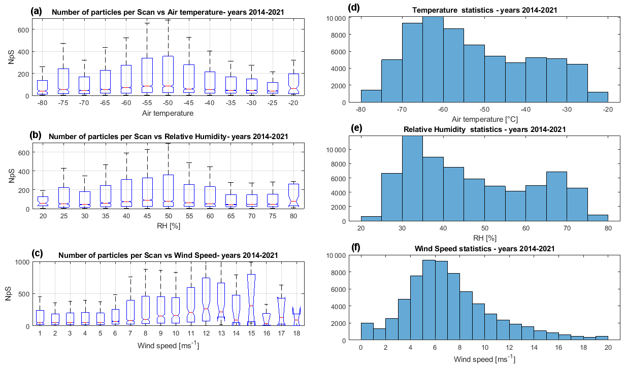
Figure 19NpS statistics in relation to (a) Tair, (b) RH, (c) wind speed. For comparison, the statistics for (d) Tair, (e) RHy, and (f) wind speed are shown for the same period (2014–2021).
Most ice particles were detected at temperatures between −60 and −45 ∘C, which are characteristic temperatures in spring and autumn. The NpS at −70 ∘C is not statistically different from the NpS at −30 ∘C. This observation shows that a statistically important number of particles is also measured at the highest DC temperatures when sublimation is expected (Sect. 3.2) to rapidly deplete the number of collected ice particles. According to the DC air temperature statistics (Fig. 19d), most particles were detected at temperatures above the median DC temperature.
Looking at NpS statistics with relative humidity (Fig. 19b), most particles were detected with relative humidity ranging from 40 % to 50 %.
Figure 19c shows NpS in relation to wind velocity: ice particles were collected by ICE-CAMERA under all wind conditions encountered in DC. Ice particles were numerically more abundant when the wind was between 7 and 15 m s−1. As the average surface wind speed at DC resulted in around ≈6 m s−1 for the measurement period (Fig. 19f), particles were collected on the DS preferentially with winds stronger than the average, a condition typically encountered in winter in coincidence with warming events (Argentini et al., 2014). These winds exceed the threshold value of 5 m s−1 for blowing snow at ICE-CAMERA altitude and may ultimately contain some drifting snow. The drop of NpS for wind speeds above 15 m s−1 (very rare in DC) is probably due to the limited attachment of snow to the DS with strong winds.
5.2 Image processing and CNN used on ICE-CAMERA data
MATLAB post-processing software, including the CNN classifier (Sect. 4.2) and measurement tools (Sect. 4.1), has been applied to the 2014–2017 ICE-CAMERA dataset. Even if the detailed analysis of these data is the task of a separate paper, a sample of the capacity of the instrument is presented in this section for the first two years of measurement (2014–2015). The total particles analysed resulted in N=553.358. The number of particles classified in the 14 classes is reported in Fig. 20. The relative rarity of trigonal plates and spheroid particles is evident.
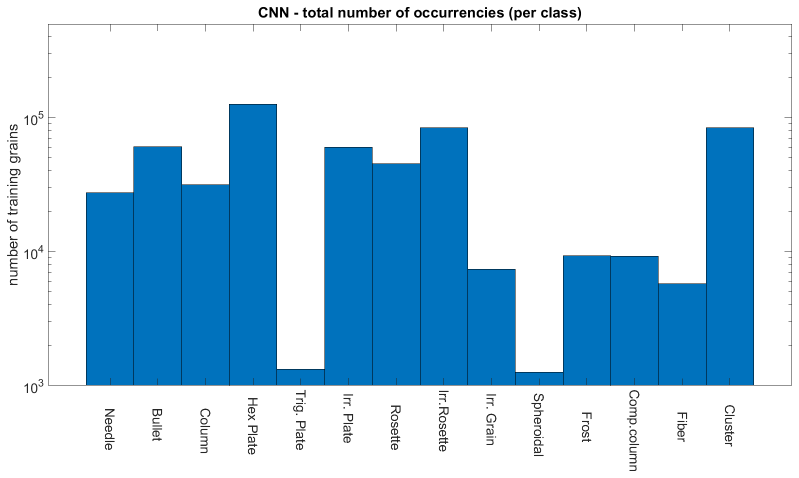
Figure 21 shows the Feret length statistics in box and whisker format. Particles classified as plates, needles, compact columns, and spheroidal and irregular grains gave an average length lower than 300 µm.The bullet and column mean lengths resulted in the 400–500 µm range, while for rosettes and irregular rosettes, it was in the 350–550 µm range.

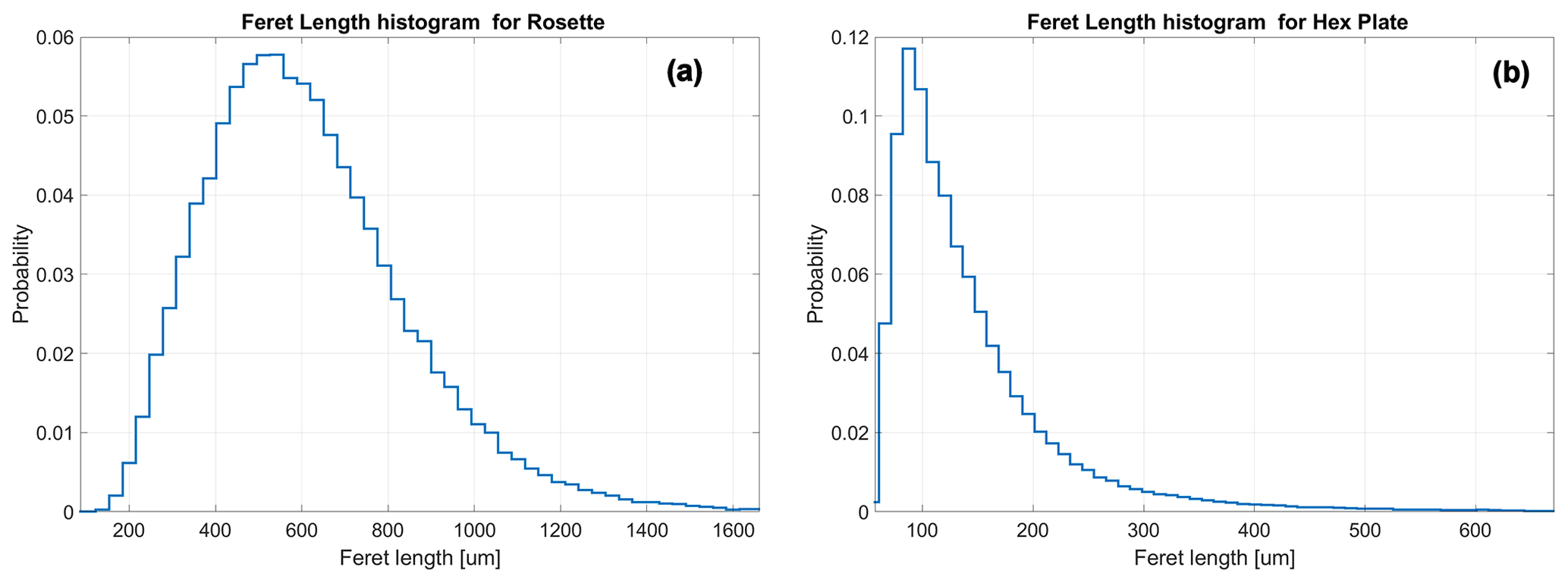
Figure 22Feret length probability distribution for (a) rosettes and (b) hex. plates. The relevant presence of small plates (D<200 µm) suggests that sublimation on the DS is not relevant, years 2014–2015.
Figure 22 shows, in detail, the probability distribution of the Feret length for plates and rosettes. For plates (Fig. 22b), the peak of the distribution is Lferet=100 µm, similar to the peak of the diamond dust (maximum) size distribution measured by Lawson et al. (2006) at SPS in summer (it must be pointed out that Lawson et al., 2006 also measured particles as small as 30 µm, while particles below 60 µm are not processed by the ICE-CAMERA software and are therefore missing from the probability distribution of Fig. 22b). This finding suggests that the sublimation of particles less than 100–200 µm in diameter during the deposition period (Sect. 3.2) is not relevant for shaping the final particle size statistics. The loss of particles in the lowest size range for sublimation cannot be quantitatively assessed from these data. Nevertheless, the first effects of sublimation are expected to be evident in the ICE-CAMERA images of small particles in the form of the loss of sharp edges, eventually leading to spheroidal shapes (Sect. 3.2). An overview of the images collected in the 2014–2015 summers (where sublimation is most likely to occur) indicates that this effect is rarely observed. Either sublimation is slower than expected from the simulations of Sect. 3.2, or what is observed in the summer images of ICE-CAMERA is just the result of the crystals felt just before the scan, with the majority of previously fallen small particles having been definitely sublimated and thus not detected by image segmentation. This ambiguity will be resolved in DC by taking a continuous series of acquisitions of DD in summer conditions. The results obtained from ICE-CAMERA for pristine rosettes (Fig. 22a) differ considerably from those of Lawson et al. (2006), because the peak of the probability distribution resulted in L=480 µm, to be compared with L=120 µm of Lawson et al. (2006). This difference is not explicable with the eventual sublimation of the smallest rosettes on the DS. Instead, this result is a realistic feature, sustained by the direct visual observation of rosettes in DC precipitation. A much greater amount of rosettes is actually observed in DC during precipitation from clouds than during diamond dust events. Even if rosettes in diamond dust are much smaller than rosettes from clouds, the numerical dominance of cloud rosettes explains the large median value of their Feret length.
Figure 23a shows the Feret's aspect ratio per class. Not surprisingly, many “rounded” classes (plates, rosettes, etc.) have an AR <2. Compact columns show a median AR close to 2.4, while columns and bullets are close to 3. The average AR for the needles was 3.2, which is lower than expected, for the reasons outlined in Sect. 4.1.3.
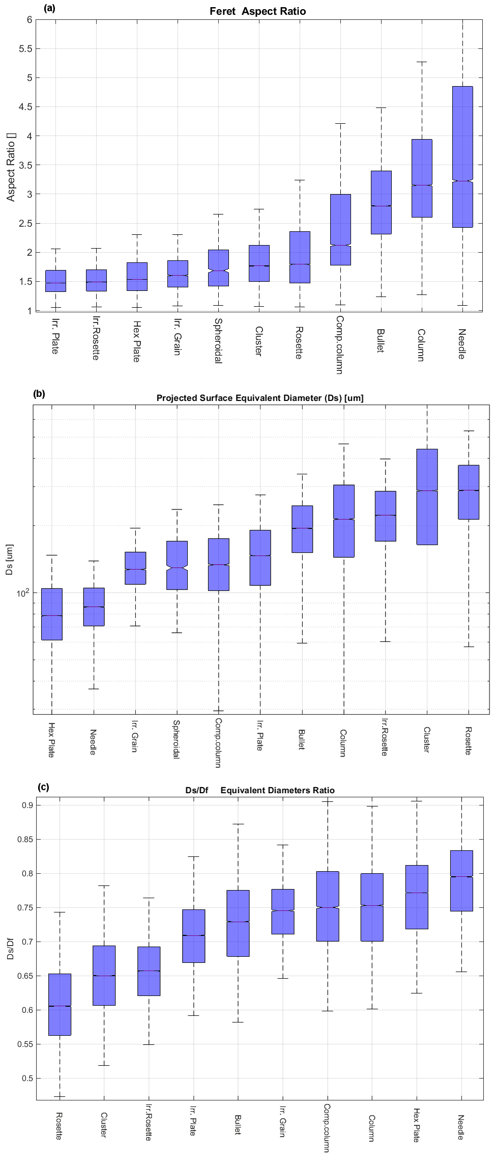
Figure 23Statistics of (a) aspect ratio, (b) projected surface-equivalent diameter (Ds), (c) ratio between surface-equivalent (Ds) and Feret-box-equivalent (Df) diameters for the years 2014–2015.
Figure 23b shows the surface-equivalent diameter Ds of the particles. Figure 23c shows the ratio between the surface-equivalent diameter (Ds) and the Feret-box-equivalent diameter (Df). The difference between the two diameters is relevant for “fluffy” particles like rosettes and clusters. For those particles, gave values of 0.6–0.65. For comparison, a round particle is expected to have a ratio of .
Using ICE-CAMERA, as well as other automated instruments, at DC was difficult. The instrument had several failures along the years, and each one was difficult to fix, at least in winter, when the instrument had to be dismounted from the roof of the shelter at −70 ∘C and eventually fixed in the local laboratory by the winter-over crew, with remote assistance from Europe. Until a few years ago, communicating with DC was limited to emails with small attachments, making remote assistance a lengthy task. Even today, connecting the rest of the world remotely with the ICE-CAMERA PC to operate the instrument software is virtually impossible. Most hardware failures in DC were due to software bugs or computer failures. Rather than having trouble with low temperatures, operating in DC meant dealing with the limited heat-dissipation of PC parts, such as power supply and hard disks; electrostatic discharge issues in low-humidity, heated environments; a lack of spare parts for most of the year; and the varied skill level of winter-over personnel. Failures in the thermal control of ICE-CAMERA caused some mechanical stress and failures in the focusing sledge, while water condensation eventually rusted the bearings of the stepper motors (all bearings were de-greased for a better low-temperature operation). The CNN used to classify ICE-CAMERA images is continually changing and improving, and the CNN training dataset increases with time as new images collected by ICE-CAMERA are used as new training ones.
ICE-CAMERA, although very similar to a simple flatbed scanner in its basic design, has represented a technical challenge for its implementation at DC. Hardware and software have been continuously and extensively modified at DC over the past five summer campaigns. The result is now a reliable instrument, running throughout the year on an hourly basis, for the statistical study of precipitation in internal polar areas. Particle size and morphology are automatically obtained, and some semi-quantitative precipitation estimates can be derived. The collected data are automatically pre-analysed, but they can be post-processed at any time, in order to follow the continuous improvements of the image processing and machine learning algorithms. The GoogleNet CNN, trained specifically for this instrument, has succeeded in classifying ICE-CAMERA images into 14 form classes, with an accuracy of more than 80 % for most of them. The instrument is particularly useful for automatically measuring the size of individual ice particles in precipitation, a process virtually impossible manually and certainly impossible on the field in DC and elsewhere on the Antarctic plateau in winter. ICE-CAMERA scans are carried out every hour. Keeping the surface of the instrument free of frost all the time and cleaning it by heating the deposition surface after each scan is paid with the possible loss of small ice particles. Particles less than 100–200 µm can disappear by sublimation before being recorded, especially in summer. This problem is complementary to the problem encountered when observing precipitation manually: when observing precipitation manually every 24 h, (as is the case of DC), the reprocessing of particles or the formation of ice and hoar artefacts cannot be prevented. In ICE-CAMERA, frost and ice regrowth are suppressed, but small particles may disappear as a result of sublimation. The effect of sublimation on particles observed with ICE-CAMERA cannot be easily quantified, given the broad range of atmospheric conditions encountered by the DS throughout the year. Images of small particles (100–200 µm) (such as plates) collected during the 2014–2015 summers rarely show evidence of early sublimation, such as edge smoothing or rounding. While encouraging specific experiments with ICE-CAMERA, this observation suggests that sublimation could be slower than predicted by simulations. ICE-CAMERA data collected since 2014 have already been statistically processed, and the results will be described in a specialised paper. Results from a subset of data (years 2014–2015) was presented in this work. As preliminary results, in DC, the rosettes were found to be significantly larger (480 µm) than those observed at SPS by Lawson et al. (2006), while the plates were of a similar size (120 µm). These results demonstrated the capability of the instrument to classify and size individual ice particles in DC precipitation. Unfortunately, only non-polluted, very cold, low-humidity, low-precipitation environments (like high mountain tops or dry polar environments) could house a similar instrument. In the presence of pollution, marine aerosols, or dust, manual cleaning of the DS would be required to remove solid particles and salts escaping sublimation. For coastal zones, the temperature is generally close to zero, making the thermal cleaning of the DS by sublimation problematic. In these environments, if an instrument like ICE-CAMERA were installed, a mechanical wiper would replace the heated glass of the current instrument. Furthermore, the CNN presented in this paper should be re-trained with different classes of ice crystals.
The CNN developed as part of this work (under Mathworks MATLAB R2020B), along with the image dataset (224×224 images for the 14 classes of particles) used for training, validation, and testing the CNN are available in the Zenodo repository at https://doi.org/10.5281/zenodo.6822140 (Del Guasta, 2022).
The author has declared that there are no competing interests.
Publisher’s note: Copernicus Publications remains neutral with regard to jurisdictional claims in published maps and institutional affiliations.
I am grateful to the Italian Antarctic Project PNRA for supporting this work with the projects ICE-CAMERA (PNRA 2009/A4.1) and PRE-REC (PNRA 2013/AC3.05). I am also grateful to the “Osservatorio Meteo-Climatologico Antartico” (PNRA 14_00100) for the Meteo data and to all the logistics staff and winter-over crews of Concordia station, all working hard to permit our scientific activity. I am also grateful to Francesco Castagnoli (INO CNR) for the initial design of the instrument.
This paper was edited by Alexis Berne and reviewed by Thomas Kuhn and one anonymous referee.
Argentini, S., Pietroni, I., Mastrantonio, G., Viola, A. P., Dargaud, G., and Petenko, I.: Observations of near surface wind speed, temperature and radiative budget at Dome C, Antarctic Plateau during 2005, Antarct. Sci., 26, 104–112, https://doi.org/10.1017/S0954102013000382, 2014.
Aristidi, E.: An analysis of temperatures and wind speeds above Dome C, Antarctica, Astron. Astrophys., 430, 739–746, https://doi.org/10.1051/0004-6361:20041876, 2005.
Bailey, M. P. and Hallett, J.: A Comprehensive Habit Diagram for Atmospheric Ice Crystals: Confirmation from the Laboratory, AIRS II, and Other Field Studies, J. Atmos. Sci., 61, 2888–2899, https://doi.org/10.1175/2009JAS2883.1, 2009.
Böhm, H. P.: A General Equation for the Terminal Fall Speed of Solid Hydrometeors, J. Atmos. Sci., 46, 2419–2427, https://doi.org/10.1175/1520-0469(1989)046<2419:AGEFTT>2.0.CO;2, 1989.
Bracci, A., Baldini, L., Roberto, N., Adirosi, E., Montopoli, M., Scarchilli, C., Grigioni, P., Ciardini, V., Levizzani, V., and Porcù, F.: Quantitative Precipitation Estimation over Antarctica Using Different Ze–SR Relationships Based on Snowfall Classification Combining Ground Observations, Remote Sens., 14, 82, https://doi.org/10.3390/rs14010082, 2022.
Bromwich, D. H.: Snowfall in high southern latitudes, Rev. Geophys., 26, 149–168, https://doi.org/10.1029/RG026i001p00149, 1988.
Chokshi, A., Tielens, A. G. G. M., and Hollenbach, D.: Dust Coagulation, Astrophys. J., 407, p. 806, https://doi.org/10.1086/172562, 1993.
Del Guasta, M.: CNN for the classification of ICE-CAMERA images of Antarctic ice particles, Zenodo [data set], https://doi.org/10.5281/zenodo.6822140, 2022.
Deng, J., Dong, W., Socher, R., Li, L.-J., Li, K., and Li, F.-F.: ImageNet: A large-scale hierarchical image database, in: 2009 IEEE Conference on Computer Vision and Pattern Recognition, Miami, FL, USA, 20–25 June 2009, IEEE, 248–255, https://doi.org/10.1109/CVPR.2009.5206848, 2009.
Eidevåg, T., Abrahamsson, P., Eng, M., and Rasmuson, A.: Modeling of dry snow adhesion during normal impact with surfaces, Powder Technol., 361, 1081–1092, https://doi.org/10.1016/j.powtec.2019.10.085, 2020
Fujita, K. and Abe, O.: Stable isotopes in daily precipitation at Dome Fuji, East Antarctica, Geophys. Res. Lett., 33, L18503, https://doi.org/10.1029/2006GL026936, 2006.
Garrett, T. J., Fallgatter, C., Shkurko, K., and Howlett, D.: Fall speed measurement and high-resolution multi-angle photography of hydrometeors in free fall, Atmos. Meas. Tech., 5, 2625–2633, https://doi.org/10.5194/amt-5-2625-2012, 2012.
Genthon, C., Veron, D. E., Vignon, E., Madeleine, J.-B., and Piard, L.: Water vapor in cold and clean atmosphere: a 3-year data set in the boundary layer of Dome C, East Antarctic Plateau, Earth Syst. Sci. Data, 14, 1571–1580, https://doi.org/10.5194/essd-14-1571-2022, 2022.
Grazioli, J., Tuia, D., Monhart, S., Schneebeli, M., Raupach, T., and Berne, A.: Hydrometeor classification from two-dimensional video disdrometer data, Atmos. Meas. Tech., 7, 2869–2882, https://doi.org/10.5194/amt-7-2869-2014, 2014.
Grazioli, J., Genthon, C., Boudevillain, B., Duran-Alarcon, C., Del Guasta, M., Madeleine, J.-B., and Berne, A.: Measurements of precipitation in Dumont d'Urville, Adélie Land, East Antarctica, The Cryosphere, 11, 1797–1811, https://doi.org/10.5194/tc-11-1797-2017, 2017a.
Grazioli, J., Madeleine, J.-B., Gallée, H., Forbes, R. M., Genthon, C., Krinner, G., and Berne, A.: Katabatic Winds Diminish Precipitation Contribution to the Antarctic Ice Mass Balance, P. Natl. Acad. SCI. USA, 114, 10858–10863, https://doi.org/10.1073/pnas.1707633114, 2017b.
Grazioli, J., Ghiggi, G., Billault-Roux, A. C., and Berne, A.: MASCDB, a database of images, descriptors and microphysical properties of individual snowflakes in free fall, Scientific Data, 9, 186, https://doi.org/10.1038/s41597-022-01269-7, 2022.
Ham, F. S.: Shape-preserving solutions of the time-dependent diffusion equation, Q. Appl. Math., 17, 137–145, https://doi.org/10.1090/qam/108196, 1959.
Heymsfield, A. J., Protat, A., Bouniol, D., Austin, R. T., Hogan, R. J., Delanoë, J., Okamoto, H., Sato, K., van Zadelhoff, G., Donovan, D. P., and Wang, Z.: Testing IWC Retrieval Methods Using Radar and Ancillary Measurements with In Situ Data, J. Appl. Meteorol. Clim., 47, 135–163, https://doi.org/10.1175/2007JAMC1606.1, 2008.
Hiley, M. J., Kulie, M. S., and Bennartz, R.: Uncertainty Analysis for CloudSat Snowfall Retrievals, J. Appl. Meteorol. Clim., 50, 399–418, 2011.
Hogan, A. W.: Summer Ice Crystal Precipitation at the South Pole, J. Appl. Meteorol., 14, 246–248, https://doi.org/10.1175/1520-0450(1975)014<0246:SICPAT>2.0.CO;2, 1975.
Hu, M. K.: Visual pattern recognition by moment invariants, IRE T. Inform. Theor., 8, 179–187, https://doi.org/10.1109/TIT.1962.1057692, 1962.
Huffman, G. J., Adler, R. F., Morrissey, M. M., Bolvin, D. T., Curtis, S., Joyce, R., McGavock, B., and Susskind, J.: Global Precipitation at One-Degree Daily Resolution from Multisatellite Observations, J. Hydrometeorol., 2, 36–50, https://doi.org/10.1175/1525-7541(2001)002<0036:GPAODD>2.0.CO;2, 2001.
Jambon-Puillet, E., Shahidzadeh, N., and Bonn, D.: Singular sublimation of ice and snow crystals, Nat. Commun., 9, 4191, https://doi.org/10.1038/s41467-018-06689-x, 2018.
Kikuchi, K. and Hogan, A. W.: Properties of Diamond Dust Type Ice Crystals Observed in Summer Season at Amundsen-Scott South Pole Station, Antarctica, J. Meteorol. Soc. Jpn. Ser. II, 57, 180–190, https://doi.org/10.2151/jmsj1965.57.2_180, 1979.
Kikuchi, K., Kameda, T., Higuchi, K., and Yamashita, A.: A global classification of snow crystals, ice crystals, and solid precipitation based on observations from middle latitudes to polar regions, Atmos. Res., 132, 460–472, https://doi.org/10.1016/j.atmosres.2013.06.006, 2013.
Konishi, H., Muramoto, K., Shiina, T., Endoh, T., and Kitano, K.: Z–R relation for graupels and aggregates observed at Syowa station, Antarctica, Proc. NIPR Symp. Polar Meteorol. Glaciol., 5, 97–103, 1992.
Lachlan-Cope, T., Ladkin, R., Turner, J., and Davison, P.: Observations of cloud and precipitation particles on the Avery Plateau, Antarctic Peninsula, Antarct. Sci., 13, 339–348, https://doi.org/10.1017/S0954102001000475, 2001.
Lamb, D. and Hobbs, P. V.: Growth Rates and Habits of Ice Crystals Grown from the Vapor Phase, J. Atmos. Sci., 28, 1506–1509, https://doi.org/10.1175/1520-0469(1971)028<1507:GRAHOI>2.0.CO;2, 1971.
Lawson, R. P., Baker, B. A., Zmarzly, P., O'Connor, D., Mo, Q., Gayet, J., and Shcherbakov, V.: Microphysical and Optical Properties of Atmospheric Ice Crystals at South Pole Station, J. Appl. Meteorol. Clim., 45, 1505–1524, https://doi.org/10.1175/JAM2421.1, 2006.
LeCun, Y., Bengio, Y., and Hinton, G.: Deep learning, Nature, 521, 436–444, https://doi.org/10.1038/nature14539, 2015.
Libbrecht, K. G.: The physics of snow crystals, Rep. Prog. Phys., 68, 855–895, https://doi.org/10.1088/0034-4885/68/4/R03, 2005.
Libbrecht, K. G.: Physical Dynamics of Ice Crystal Growth, Annu. Rev. Mater. Res., 47, 271–295, https://doi.org/10.1146/annurev-matsci-070616-124135, 2017.
Libois, Q., Picard, G., Arnaud, L., Morin, S., and Brun, E.: Modeling the impact of snow drift on the decameter-scale variability of snow properties on the Antarctic Plateau, J. Geophys. Res.-Atmos., 119, 662–681, https://doi.org/10.1002/2014JD022361, 2014.
Lindqvist, H., Muinonen, K., Nousiainen, T., Um, J., McFarquhar, G. M., Haapanala, P., Makkonen, R., and Hakkarainen, H.: Ice-cloud particle habit classification using principal components, J. Geophys. Res., 117, D16206, https://doi.org/10.1029/2012JD017573, 2012.
Liu, G.: Deriving snow cloud characteristics from cloudsat observations, J. Geophys. Res.-Atmos., 113, D00A09, https://doi.org/10.1029/2007JD009766, 2008.
Magono, C. and Lee, C. W.: Meteorological classification of natural snow crystals, Journal of the Faculty of Science, Hokkaido University, Series 7, Geophysics, 2, 321–335, 1966.
Nelson, J.: Sublimation of Ice Crystals, J. Atmos. Sci., 55, 910–919, https://doi.org/10.1175/1520-0469(1998)055<0910:SOIC>2.0.CO;2, 1988.
Newman, A. J., Kucera, P. A., and Bliven, L. F.: Presenting the Snowflake Video Imager (SVI), J. Atmos. Ocean. Tech., 26, 167–179, https://doi.org/10.1175/2008JTECHA1148.1, 2009.
Ohtake, T. and Yogi, T.: Winter ice crystals at the South Pole, Antarct. J. US, 14, 201–203, 1979.
Palerme, C., Kay, J. E., Genthon, C., L'Ecuyer, T., Wood, N. B., and Claud, C.: How much snow falls on the Antarctic ice sheet?, The Cryosphere, 8, 1577–1587, https://doi.org/10.5194/tc-8-1577-2014, 2014.
Palerme, C., Claud, C., Dufour, A., Genthon, C., Wood, N. B., and L'Ecuyer, T.: Evaluation of Antarctic snowfall in global meteorological reanalyses, Atmos. Res., 190, 104–112, https://doi.org/10.1016/j.atmosres.2017.02.015, 2017.
Palm, S. P., Yang, Y., and Vinay, K.: New Perspectives on Blowing Snow in Antarctica and Implications for Ice Sheet Mass Balance, in: Antarctica – A Key To Global Change, edited by: Kanao, M., Toyokuni, G., and Yamamoto, M., IntechOpen, https://doi.org/10.5772/intechopen.81319, 2018
Pratt, W. K.: Digital Image Processing: PIKS Scientific Inside, 4th edn., John Wiley & Sons, Inc., Los Altos, California, https://doi.org/10.1002/0470097434, 2007.
Praz, C., Roulet, Y.-A., and Berne, A.: Solid hydrometeor classification and riming degree estimation from pictures collected with a Multi-Angle Snowflake Camera, Atmos. Meas. Tech., 10, 1335–1357, https://doi.org/10.5194/amt-10-1335-2017, 2017.
Russ, J. C. and Brent Neal, F.: The Image Processing Handbook, 7th edn., CRC Press, 1053 pp., https://doi.org/10.1201/b18983, 2017.
Ryzhkin, I. A. and Petrenko, V. F.: Physical Mechanisms Responsible for Ice Adhesion, J. Phys. Chem. B, 101, 6267–6270, https://doi.org/10.1021/jp9632145, 1977.
Santachiara, G., Belosi, F., and Prodi, F.: Ice crystal precipitation at Dome C site (East Antarctica), Atmos. Res., 167, 108–117, https://doi.org/10.1016/j.atmosres.2015.08.006, 2016.
Satow, K.: Observations on the Shapes of Snow Crystals in the Summer Season in Mizuho Plateau, Antarctica, Memoirs of National Institute of Polar Research, Special issue, 29, 103–109, 1983.
Schlosser, E., Dittmann, A., Stenni, B., Powers, J. G., Manning, K. W., Masson-Delmotte, V., Valt, M., Cagnati, A., Grigioni, P., and Scarchilli, C.: The influence of the synoptic regime on stable water isotopes in precipitation at Dome C, East Antarctica, The Cryosphere, 11, 2345–2361, https://doi.org/10.5194/tc-11-2345-2017, 2017.
Schmidhuber, J.: Deep Learning in Neural Networks: An Overview, Neural Networks, 61, 85–117, https://doi.org/10.1016/j.neunet.2014.09.003, 2014.
Schneider, U., Finger, P., Meyer-Christoffer, A., Rustemeier, E., Ziese, M., and Becker, A.: Evaluating the Hydrological Cycle over Land Using the Newly-Corrected Precipitation Climatology from the Global Precipitation Climatology Centre (GPCC), Atmosphere, 8, 52, https://doi.org/10.3390/atmos8030052, 2017.
Shimizu, H.: Long prism “Crystals observed in the precipitation in Antarctica”, J. Meteorol. Soc. Jpn., 41, 305–307, https://doi.org/10.2151/jmsj1923.41.5_305, 1963.
Shorten, C. and Khoshgoftaar, T. M.: A survey on Image Data Augmentation for Deep Learning, Journal of Big Data, 6, 60, https://doi.org/10.1186/s40537-019-0197-0, 2019.
Smiley, V. N., Whitcomb, B. M., Morley, B. M., and Warburton, J. A.: Lidar Determinations of Atmospheric Ice Crystal Layers at South Pole during Clear-Sky Precipitation, J. Appl. Meteorol., 19, 1074–1090, 1980.
Souverijns, N., Gossart, A., Lhermitte, S., Gorodetskaya, I. V., Kneifel, S., Maahn, M., Bliven, F. L., and van Lipzig, P. M.: Estimating radar reflectivity - Snowfall rate relationships and their uncertainties over Antarctica by combining disdrometer and radar observations, Atmos. Res., 196, 211–223, https://doi.org/10.1016/j.atmosres.2017.06.001, 2017.
Szegedy, C., Liu, W., Jia, Y., Sermanet, P., Reed, S., Anguelov, D., Erhan, D., Vanhoucke, V., and Rabinovich, A.: Going deeper with convolutions, in: 2015 IEEE Conference on Computer Vision and Pattern Recognition (CVPR), Boston, MA, 7–12 June 2015, IEEE, 1–9, https://doi.org/10.1109/CVPR.2015.7298594, 2015.
Tremblin, P., Minier, V., Schneider, N., Durand, G. Al., Ashley, M. C. B., Lawrence, J. S., Luong-Van, D. M., Storey, J. W. V., Durand, G. An., Reinert, Y., Veyssiere, C., Walter, C., Ade, P., Calisse, P. G., Challita, Z., Fossat, E., Sabbatini, L., Pellegrini, A., Ricaud, P., and Urban, J.: Site testing for submillimetre astronomy at Dome C, Antarctica, Astron. Astrophys., 535, A112, https://doi.org/10.1051/0004-6361/201117345, 2011.
Vignon, E., Genthon, C., Barral, H., Amory, C., Picard, G., Gallée, H., Casasanta, G., and Argentini, S.: Momentum- and Heat-Flux Parametrization at Dome C, Antarctica: A Sensitivity Study, Bound.-Lay. Meteorol., 162, 341–367, https://doi.org/10.1007/s10546-016-0192-3, 2017.
Walden, V. P., Warren, S. G., and Tuttle, E.: Atmospheric Ice Crystals over the Antarctic Plateau in Winter, J. Appl. Meteorol., 42, 1391–1405, https://doi.org/10.1175/1520-0450(2003)042<1391:AICOTA>2.0.CO;2, 2003.
Walton, W. H.: Feret's Statistical Diameter as a Measure of Particle Size, Nature, 162, 329–330, https://doi.org/10.1038/162329b0, 1948.
Wood, N., L'Ecuyer, T., Heymsfield, A., and Stephens, G.: Microphysical Constraints on Millimeter-Wavelength Scattering Properties of Snow Particles, J. Appl. Meteorol. Clim., 54, 909–931, https://doi.org/10.1175/JAMC-D-14-0137.1, 2015.
Xiao, H., Zhang, F., He, Q., Liu, P., Yan, F., Miao, L., and Yang, Z.: Classification of ice crystal habits observed from airborne Cloud ParticleImager by deep transfer learning, Earth and Space Science, 6, 1877–1886, https://doi.org/10.1029/2019EA000636, 2019.
Zheleznyak, A. G. and Sidorov, V. G.: Flatbed scanner as an instrument for physical studies, St. Petersburg Polytechnical University Journal: Physics and Mathematics, 1, 134–141, https://doi.org/10.1016/j.spjpm.2015.04.001, 2015.