the Creative Commons Attribution 4.0 License.
the Creative Commons Attribution 4.0 License.
 | 08 Dec 2022
Validation of the Aeolus L2B wind product with airborne wind lidar measurements in the polar North Atlantic region and in the tropics
Benjamin Witschas
Christian Lemmerz
Alexander Geiß
Oliver Lux
Uwe Marksteiner
Stephan Rahm
Oliver Reitebuch
Andreas Schäfler
Fabian Weiler
During the first 3 years of the European Space Agency's Aeolus mission, the German Aerospace Center (Deutsches Zentrum für Luft- und Raumfahrt, DLR) performed four airborne campaigns deploying two different Doppler wind lidars (DWL) on board the DLR Falcon aircraft, aiming to validate the quality of the recent Aeolus Level 2B (L2B) wind data product (processor baseline 11 and 12). The first two campaigns, WindVal III (November–December 2018) and AVATAR-E (Aeolus Validation Through Airborne Lidars in Europe, May and June 2019), were conducted in Europe and provided first insights into the data quality at the beginning of the mission phase. The two later campaigns, AVATAR-I (Aeolus Validation Through Airborne Lidars in Iceland) and AVATAR-T (Aeolus Validation Through Airborne Lidars in the Tropics), were performed in regions of particular interest for the Aeolus validation: AVATAR-I was conducted from Keflavik, Iceland, between 9 September and 1 October 2019 to sample the high wind speeds in the vicinity of the polar jet stream; AVATAR-T was carried out from Sal, Cape Verde, between 6 and 28 September 2021 to measure winds in the Saharan dust-laden African easterly jet. Altogether, 10 Aeolus underflights were performed during AVATAR-I and 11 underflights during AVATAR-T, covering about 8000 and 11 000 km along the Aeolus measurement track, respectively. Based on these collocated measurements, statistical comparisons of Aeolus data with the reference lidar (2 µm DWL) as well as with in situ measurements by the Falcon were performed to determine the systematic and random errors of Rayleigh-clear and Mie-cloudy winds that are contained in the Aeolus L2B product. It is demonstrated that the systematic error almost fulfills the mission requirement of being below 0.7 m s−1 for both Rayleigh-clear and Mie-cloudy winds. The random error is shown to vary between 5.5 and 7.1 m s−1 for Rayleigh-clear winds and is thus larger than specified (2.5 m s−1), whereas it is close to the specifications for Mie-cloudy winds (2.7 to 2.9 m s−1). In addition, the dependency of the systematic and random errors on the actual wind speed, the geolocation, the scattering ratio, and the time difference between 2 µm DWL observation and satellite overflight is investigated and discussed. Thus, this work contributes to the characterization of the Aeolus data quality in different meteorological situations and allows one to investigate wind retrieval algorithm improvements for reprocessed Aeolus data sets.
- Article
(7827 KB) - Full-text XML
- BibTeX
- EndNote


On 22 August 2018, the first ever spaceborne Doppler wind lidar Aeolus, developed by the European Space Agency (ESA), was launched into space to circle the Earth on a sun-synchronous orbit at about 320 km altitude, with a repeat cycle of 7 d (e.g., ESA, 1999, 2008; Stoffelen et al., 2005; Reitebuch, 2012; Horányi et al., 2015). Since then, Aeolus has been providing profiles of the wind vector component along the instrument's line-of-sight (LOS) direction from the ground up to about 30 km in the stratosphere (e.g., Kanitz et al., 2019; Reitebuch et al., 2020; Straume et al., 2020), primarily aiming to improve numerical weather prediction (NWP) (e.g., Weissmann and Cardinali, 2007; Tan et al., 2007; Marseille et al., 2008; Horányi et al., 2015; Rennie et al., 2021). In particular, wind profiles acquired over the Southern Hemisphere, the tropics, and the oceans contribute to closing large gaps in the availability of wind data in the global observing system (Baker et al., 2014). For the use of Aeolus observations in NWP models, a detailed characterization of the data quality as well as the minimization of systematic errors are crucial. Thus, several scientific and technical studies have been performed and published in the meantime, addressing the performance of ALADIN (Atmospheric LAser Doppler INstrument) on board Aeolus and the quality of the wind data products (e.g., Bedka et al., 2021; Martin et al., 2021; Baars et al., 2020; Guo et al., 2021; Zuo et al., 2022; Wu et al., 2022; Chou et al., 2022; Belova et al., 2021).
The German Aerospace Center (Deutsches Zentrum für Luft- und Raumfahrt, DLR) has performed four airborne calibration and validation (CalVal) campaigns since the launch of Aeolus, deploying two different Doppler wind lidars (DWLs) on board the DLR Falcon aircraft, aiming to validate the quality of the Level 2B (L2B) wind data product. During the first two campaigns, WindVal III (5 November until 5 December 2018) and AVATAR-E (6 May until 6 June 2019), which were conducted from the DLR site in Oberpfaffenhofen, Germany, 10 satellite underflights covered more than 7500 km along the Aeolus track. The performed measurements gave first insights into the quality of the early-phase Aeolus wind product. Based on collocated measurements with the ALADIN airborne demonstrator (A2D) (Reitebuch et al., 2009) during the WindVal III campaign, a statistical comparison against Aeolus data revealed a positive systematic error of 2.6 m s−1 for the Aeolus Rayleigh-clear winds and a corresponding random error of 3.6 m s−1 (Lux et al., 2020). These results were confirmed (Witschas et al., 2020) by a comparison with precise wind speed and wind direction measurements performed with DLR's 2 µm DWL (Witschas et al., 2017). The mean systematic errors of the Aeolus winds with respect to 2 µm DWL observations were determined to be 2.1 m s−1 (Rayleigh-clear) and 2.3 m s−1 (Mie-cloudy). The corresponding random errors were found to be 3.9 and 2.0 m s−1. Additionally, Witschas et al. (2020) discussed results from the subsequent AVATAR-E campaign, yielding systematic errors of −4.6 m s−1 (Rayleigh-clear) and −0.2 m s−1 (Mie-cloudy). The corresponding random errors were 4.3 and 2.0 m s−1. The larger systematic errors observed for both campaign data sets were related to small temperature fluctuations across the 1.5 m diameter primary mirror of the Aeolus telescope, which caused varying wind biases along the orbit of up to 8 m s−1 (Rennie and Isaksen, 2020; Rennie et al., 2021; Weiler et al., 2021b). In the meantime (since 20 April 2020), the impact of these thermal fluctuations is successfully corrected in the Aeolus processor by means of ECMWF (European Centre for Medium-Range Weather Forecasts) model-equivalent winds. Furthermore, the Aeolus detector showed anomalies in the dark current on single pixels, which led to wind speed errors of up to 30 m s−1, depending on the strength of the atmospheric signal (Weiler et al., 2021a). A corresponding correction scheme that was implemented in the Aeolus data processor on 14 June 2019 significantly reduced the impact of these hot pixels on the wind data quality.
The enhanced systematic error of Aeolus wind data in the early mission phase was further demonstrated by other data sets. For instance, in April 2019, NASA conducted five research flights over the eastern Pacific Ocean with their DC-8 aircraft, equipped with a heterodyne-detection Doppler wind lidar and a water vapor lidar (Bedka et al., 2021), which revealed a systematic error of 1.2 m s−1 (Rayleigh-clear) and 2.0 m s−1 (Mie-cloudy). The corresponding random errors were determined to be 5.1 and 4.7 m s−1. Baars et al. (2020) used radiosonde data launched during the Polarstern research vessel cruise from Bremerhaven to Cape Town in November–December 2018 and determined the systematic and random error of the Rayleigh-clear winds to be 1.5 and 3.3 m s−1, respectively. Martin et al. (2021) performed a statistical validation of Aeolus observations using collocated radiosonde measurements and NWP forecast equivalents from two different global models, the ICOsahedral Nonhydrostatic model (ICON) of Deutscher Wetterdienst (DWD) and the ECMWF Integrated Forecast System (IFS) model, as reference data. The analysis, which covered the Northern Hemisphere in the time period August 2018 to December 2019, showed strong spatial variations of the Aeolus wind bias and differences between ascending and descending orbits, in agreement with the aforementioned thermal fluctuations on the Aeolus telescope mirror, which are different for the respective orbit direction and were not corrected in that timeframe. The mean absolute bias for the selected validation area is found to be in the range of 1.8–2.3 m s−1 (Rayleigh-clear) and 1.3–1.9 m s−1 (Mie-cloudy). In addition, radar wind profiler (RWP) measurements over China, Australia, and Japan were used for Aeolus validation. In combination with ground-based lidar and radiosonde measurements, a comparison of RWP measurements over Japan against Aeolus data demonstrates that the systematic error is significantly reduced with improved algorithms in the Aeolus L2B data processor (from version L2B02 to L2B10), which is due to the implemented telescope mirror temperature correction and other improvements, such as the correction of hot pixels on the detector (Iwai et al., 2021). In particular, for the L2B02 and L2B10 period, the systematic errors were determined to be 0.5 to 1.7 and −0.8 to 0.5 m s−1 (Rayleigh-clear) as well as 1.6 to 2.4 and −0.7 to 0.2 m s−1 (Mie-cloudy), respectively. The corresponding random errors were 6.7 and 6.4 m s−1 (Rayleigh-clear) as well as 5.1 and 4.8 m s−1 (Mie-cloudy). The successful implementation of error corrections in the Aeolus L2B processor was also demonstrated by Guo et al. (2021) and Zuo et al. (2022), who used RWP measurements over China from April to July 2020 and over Australia from October 2020 until March 2021, respectively, to reveal a smaller mean systematic error of −0.6 m s−1 (Rayleigh-clear) and −0.3 m s−1 (Mie-cloudy) or 0.7 m s−1 for both Rayleigh-clear and Mie-cloudy winds. Besides that, Wu et al. (2022) used ground-based DWL measurements in the timeframe of January–December 2020 and determined systematic errors of −1.2 m s−1 (Rayleigh-clear) and −0.3 m s−1 (Mie-cloudy) and random errors of 5.8 m s−1 (Rayleigh-clear) and 2.6 m s−1 (Mie-cloudy), respectively. A summary of the validation results from different CalVal campaigns is given in Table 1, containing the time period of the respective campaigns, the L2B processor version that was operational within this time period, the systematic error μ and random error σ of Rayleigh-clear and Mie-cloudy winds, and the reference instrument that was used.
Witschas et al. (2020)Lux et al. (2020)Baars et al. (2020)Iwai et al. (2021)Bedka et al. (2021)Witschas et al. (2020)Martin et al. (2021)Wu et al. (2022)Iwai et al. (2021)Guo et al. (2021)Zuo et al. (2022)Table 1Overview of Aeolus L2B validation results from different campaign data sets.
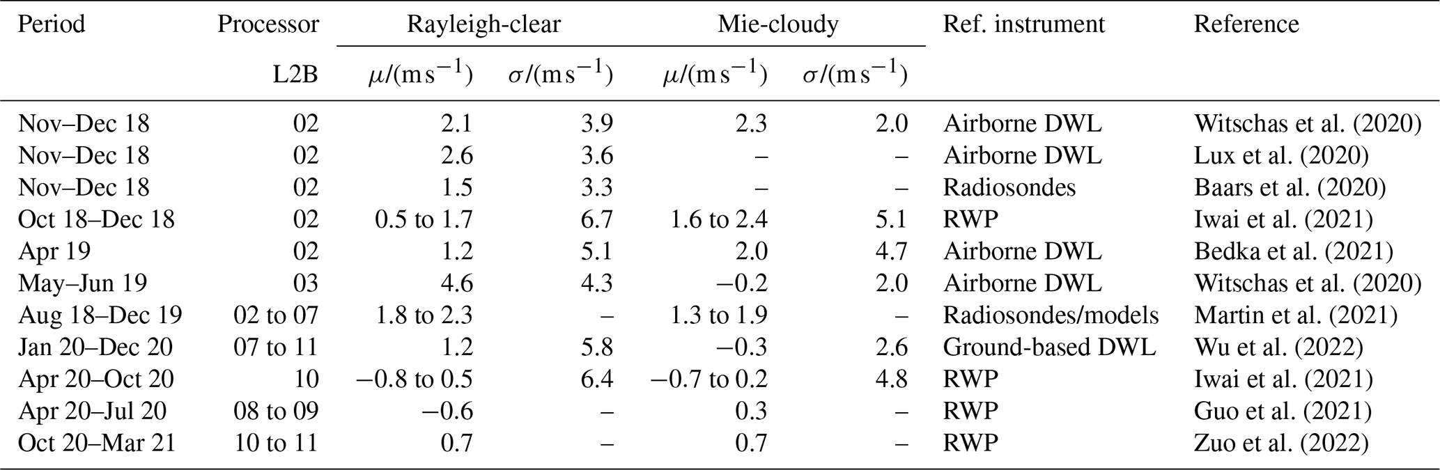
μ – systematic error; σ – random error; DWL – Doppler wind lidar; RWP – radio wind profiler.
In this paper, the aforementioned work of other CalVal teams is extended by the analysis of the L2B wind quality in two dedicated regions over the North Atlantic, namely the extratropical polar jet stream and the region of tropical winds affected by dust transport; both regions are of particular importance to NWP (Tan and Andersson, 2005; Schäfler et al., 2020). In particular, two airborne campaigns with the Falcon aircraft being equipped with the A2D and the 2 µm DWL were conducted, namely the AVATAR-I campaign (Keflavik, Iceland, 9 September until 1 October 2019) and the AVATAR-T campaign (Sal, Cape Verde, 6 until 28 September 2021). The 2 µm DWL data set acquired during these two campaigns is used to derive the systematic and random error of Rayleigh-clear and Mie-cloudy winds and to investigate their dependency on different quantities such as the actual wind speed, the geolocation, the scattering ratio, and the time difference between 2 µm DWL observation and satellite overflight for a more detailed error characterization. In addition to the 2 µm DWL measurements, in situ observations with the Falcon nose boom are used for comparison. A dedicated study of the Aeolus measurement principle, its calibration procedures, and its retrieval algorithms is performed based on A2D observations, as separately discussed in Lux et al. (2020, 2022a).
The paper is structured as follows. In Sect. 2, an overview is given about the AVATAR-I and AVATAR-T campaigns, followed by an introduction of the instruments used in this study (Sect. 3), namely ALADIN on board Aeolus (Sect. 3.1), DLR's 2 µm DWL (Sect. 3.2), and the flow angle sensor in Falcon's nose boom (Sect. 3.3). Afterwards, the data processing steps are discussed in Sect. 4, containing the explanation of the averaging procedures (Sect. 4.1), the introduction of the quantities used for the statistical comparison (Sect. 4.2), and an explanation of the quality control that is applied to the Aeolus data (Sect. 4.3). In Sect. 5, the results of the statistical comparison are discussed for the systematic errors (Sect. 5.1) as well as for the random errors (Sect. 5.2). The results retrieved from the comparison against Falcon in situ measurements are separately treated in Sect. 5.3. In Sect. 6, the Aeolus error dependency on various quantities is revealed for Rayleigh-clear (Sect. 6.1) and Mie-cloudy winds (Sect. 6.2), followed by a summary of the results of this study given in Sect. 7.
In this study, results from the AVATAR-I (Aeolus Validation Through Airborne Lidars in Iceland) campaign, conducted from 9 September to 1 October 2019 from Keflavik in Iceland, and from the AVATAR-T (Aeolus Validation Through Airborne Lidars in the Tropics) campaign, performed from 6 to 28 September 2021 in Sal, Cape Verde, are presented. AVATAR-T was DLR's contribution to the international Joint Aeolus Tropical Atlantic campaign (JATAC) initiated by ESA, which combined several airborne participants such as the French SAFIRE Falcon 20 and the NASA DC-8 (based on the US Virgin Islands) with a number of ground-based measurements and the deployment of a light aircraft with aerosol in situ equipment from the University of Nova Gorica (Slovenia), both performed from Mindelo on the island of São Vincente, Cape Verde (Fehr et al., 2021). During both campaigns, the DLR Falcon was equipped with two well-established wind lidar systems that have already been deployed in several Aeolus pre-launch campaigns (Marksteiner et al., 2018; Schäfler et al., 2018; Lux et al., 2018). In particular, the Falcon hosted the A2D, which is a prototype of the ALADIN instrument, with a representative design and measurement principle (Reitebuch et al., 2009). Hence, the A2D is the optimal instrument to validate the Aeolus measurement principle, calibration procedures, and retrieval algorithms. In addition to the A2D, a heterodyne-detection wind lidar (2 µm DWL) with a high sensitivity to particulate returns was flown and acted as a reference system (Witschas et al., 2017) to validate the quality of the Aeolus wind product.
During AVATAR-I, a total of 10 Aeolus underflights were performed, including 4 flights along descending orbits which were not possible during previous campaigns (see also Fig. 1, left, and Table 2). The first underflight along an ascending orbit could already be performed on the transfer from Oberpfaffenhofen to Keflavik after a refueling stop-over in Prestwick, UK. During the 10 underpasses, about 8000 km of the Aeolus measurement track was sampled by the two lidars. In contrast to the previous CalVal campaigns, Aeolus operated with a dedicated range bin setting (RBS) that was exclusively applied in the area around Iceland during the AVATAR-I timeframe, as shown in Fig. 2, left. The setting was optimized to a higher resolution of 500 m throughout the troposphere for both the Rayleigh and the Mie channel and thus provided a better overlap with more data points between the observations of Aeolus and the airborne wind lidars at the expense of an increased noise level. Furthermore, the high wind speeds in the vicinity of the jet stream were better resolved. Above 10 km, the three Rayleigh range bins were set to a 1 km size to extend the maximum sampled altitude to about 13 km and, with that, to ensure that winds in the lower stratosphere were also measured.

Figure 1Flight tracks of the Falcon aircraft during the AVATAR-I campaign (left) and the AVATAR-T campaign (right). Each color represents a single flight.
During AVATAR-T, 11 Aeolus underflights could be performed, covering about 11 000 km of the Aeolus measurement track (see also Fig. 1, right, and Table 2). Six of these flights were performed along ascending orbits and five along descending orbits in the morning hours. During AVATAR-T, situations with Saharan dust transport together with moderate wind cases could be targeted, making the AVATAR-T data set valuable for investigating the impact of aerosols, especially on the Rayleigh-clear wind product. Due to the decreasing performance of Aeolus and the resulting lower signal levels, it was not possible to apply a high-resolution RBS, as this would have led to noise levels that were too large. Hence, the range bin size was kept at 500 m in the lower boundary layer and was increased to 750 m in the lower troposphere, being a compromise between signal level and resolution of the usually aerosol-loaded Saharan air layer (SAL) prominent at these altitudes. In the upper troposphere and lower stratosphere, the range gates were set to 1 km (see also Fig. 2, right).

Figure 2Aeolus range bin settings (RBSs) for the Rayleigh and Mie channel applied during the AVATAR-I and AVATAR-T campaigns. The actual range bin size is color coded, and the gray area indicates the altitudes that are usually sampled by the airborne lidars on board the Falcon aircraft.
An overview of the tracks of all flights performed during AVATAR-I and AVATAR-T is given in Fig. 1 and Table 2. The latter one also provides information about the overall duration of the research flights as well as on the start and stop times and geolocations of the Aeolus underflight, which allows for an easier access to the relevant satellite wind data for comparison. Additionally, the number of Aeolus observations that could be validated by the 2 µm DWL is given for both Rayleigh-clear and Mie-cloudy winds. It can be seen that the 2 µm DWL was degrading during the AVATAR-T campaign, leading to very low data coverage for the last six research flights (see also Sect. 5). The uncertainties of the 2 µm DWL observations are, however, not affected thanks to the heterodyne-detection measurement principle of the system.
Table 2Overview of Aeolus underflights performed during the AVATAR-I and the AVATAR-T campaigns.
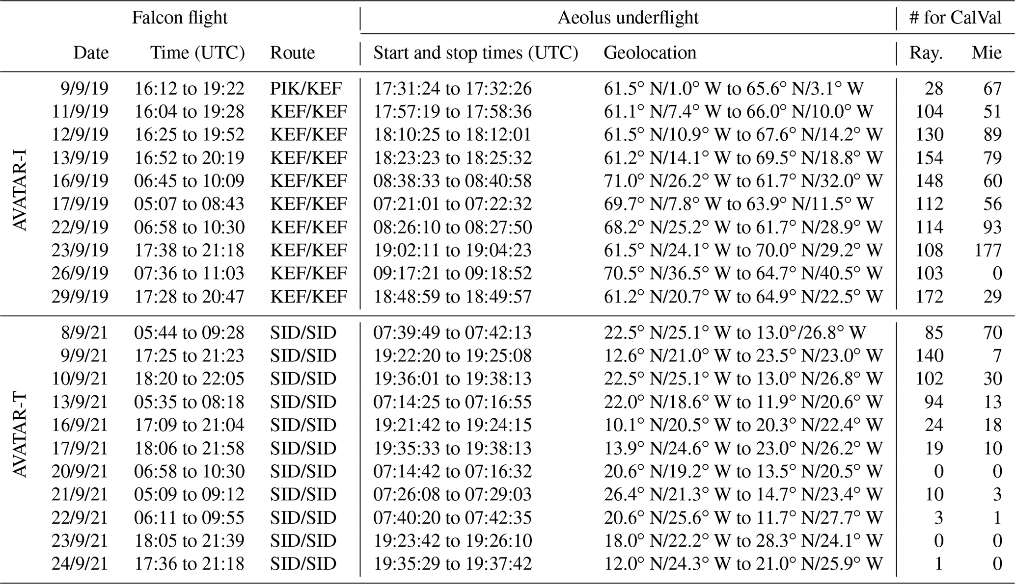
The time gives the duration between takeoff and landing. The flight route is indicated by the IATA (International Air Transport Association) airport code. PIK: Prestwick airport; KEF: Keflavik airport; SID: Amilcar Cabral airport.
3.1 Aeolus and ALADIN
The Aeolus satellite has a weight of 1360 kg, a launch configuration dimension of , and a deployable solar array that provides a power of 2.4 kW. Aeolus carries a single payload, ALADIN, which is a direct detection wind lidar operating at an ultraviolet wavelength of 354.8 nm. ALADIN emits short laser pulses (≈40 to 70 mJ, 50.5 Hz) down to the atmosphere, where a few of the photons are backscattered on air molecules, aerosols, and hydrometeors. The backscattered light is collected with a 1.5 m diameter Cassegrain telescope and directed to the optical receiver that is used to detect the Doppler frequency shift of the backscattered light from which the wind velocity can be calculated in LOS direction at different altitudes. To do so, ALADIN is equipped with two different frequency discriminators, namely a Fizeau interferometer that analyzes the frequency shift of the narrowband particulate backscatter signal by means of the so-called fringe imaging technique (McKay, 2002) and two sequentially coupled Fabry–Pérot interferometers that analyze the frequency shift of the broadband molecular return signal by means of the so-called double-edge technique (Chanin et al., 1989; Flesia and Korb, 1999; Gentry et al., 2000).
Both the Rayleigh and Mie channels sample the backscatter signal in a time-resolved manner, leading to 24 bins with a vertical resolution that can vary between 0.25 and 2.0 km (see also Fig. 2). Depending on the number of averaged measurements, which have a horizontal resolution of about 3 km, the horizontal resolution of the wind observations is usually 90 km for the Rayleigh channel (Rayleigh-clear winds) and 10 km for the Mie channel (Mie-cloudy winds). Furthermore, due to the high-spectral-resolution receiver configuration, information on the vertical distribution of aerosol and cloud optical properties such as backscatter and extinction coefficients can be retrieved (Ansmann et al., 2007; Flamant et al., 2008; Flament et al., 2021; Feofilov et al., 2022). Further information about the Aeolus satellite, the ALADIN instrument, and the retrieval algorithms can be found in other sources (e.g., ESA, 1999; Reitebuch, 2012; Reitebuch et al., 2020; Kanitz et al., 2019; Straume et al., 2018, 2020).
The data of Aeolus are provided in different product levels containing different types of information (e.g., Tan et al., 2008a, 2017; ESA, 2016; Rennie, 2018). The Level 0 data contain the raw data of ALADIN as well as the instrument housekeeping data and the housekeeping data of the satellite platform. The Level 1B (L1B) data provide processed ground echo data and preliminary horizontal LOS (HLOS) wind observations that have not been corrected for atmospheric temperature and pressure (Reitebuch et al., 2018). The L2B data contain the time series of fully processed profiles of HLOS winds along the satellite orbit. L2B Rayleigh wind data are corrected for atmospheric temperature T and pressure p, which is needed to avoid systematic errors (Dabas et al., 2008). As the Rayleigh–Brillouin spectrum of the molecular scattered light depends on T and p (Witschas et al., 2010, 2014; Witschas, 2011a, b), any differences in either of the two quantities between the geographical location of the instrument response calibration and the one of the actual wind observation have to be taken into account. L2B data are used by the ECMWF for NWP (Tan et al., 2017; Rennie, 2018) and for the validation by means of 2 µm DWL and Falcon in situ wind observations, as presented in Sect. 5. It is worth mentioning that the sign of the HLOS winds is defined such that it is positive for winds blowing away from the satellite LOS. For instance, for an ascending orbit, when the satellite moves from south to north and when the laser is pointing eastwards, westerly winds lead to positive HLOS winds. Furthermore, the L2B winds are classified by means of the optical properties of the atmosphere into Rayleigh-clear winds, indicating wind observations in aerosol-poor atmosphere, and Mie-cloudy winds, indicating winds acquired from particulate backscatter, predominately from clouds or ground returns. There are also Rayleigh-cloudy and Mie-clear winds available in the data product, which are not further discussed within this study.
Both the L1B and L2B processors are continuously updated, modified, and improved. Thus, data processed with different processor versions may result in different HLOS winds. In this study, the second reprocessed data set (processor baseline 11 – L2B processor version L2bP 3.40) is used for the AVATAR-I timeframe. For AVATAR-T, the near-real-time (NRT) data which are used in this study were processed with processor baseline 12 (L2bP 3.50). As only minor modifications have been applied between baseline 11 and 12, the different processor versions are not expected to have a significant impact on the results from the two different campaign data sets.
3.2 The airborne 2 µm DWL
The 2 µm DWL has been operated by DLR for more than 20 years and has been deployed in several ground and airborne field campaigns for measuring, for instance, aircraft wake vortices (Köpp et al., 2004), aerosol optical properties (Chouza et al., 2015, 2017), horizontal wind speeds over the Atlantic Ocean as input data for assimilation experiments (Weissmann et al., 2005; Schäfler et al., 2018), and horizontal as well as vertical wind speeds to study the life cycle of gravity waves (Witschas et al., 2017, 2022). In addition, the system was applied in several Aeolus pre-launch campaigns conducted within the last 10 years (e.g., Marksteiner et al., 2018; Lux et al., 2018).
The 2 µm DWL is a heterodyne-detection wind lidar system based on a Tm:LuAG laser operating at a wavelength of 2022.54 nm (vacuum), a laser pulse energy of 1 to 2 mJ, and a pulse repetition rate of 500 Hz, ensuring eye-safe operation. The system is composed of three main units, namely (1) a transceiver head containing the laser, an 11 cm afocal telescope, receiver optics, detectors, and a double-wedge scanner, enabling the steering of the laser beam to any position within a 30∘ cone angle; (2) a power supply and the cooling unit of the laser, mounted in a separate rack; and (3) a rack containing the data acquisition unit and the control electronics. For a more detailed description of the 2 µm DWL, including a listing of the system specifications, refer to Witschas et al. (2017).
To measure the three-dimensional wind speed and direction, the velocity–azimuth display (VAD) scan technique is applied (Browning and Wexler, 1968). That is, a conical step-and-stare scan around the vertical axes with an off-nadir angle of 20∘ is performed for 21 LOS positions, separated by 18∘ in azimuth direction. Considering a 1 s averaging time for each LOS measurement and an additional second in order to change the laser beam pointing direction, one scanner revolution takes about 42 s. By further taking into account the aircraft cruise speed of about 200 m s−1, the horizontal resolution of 2 µm DWL wind observations is about 8.4 km, depending on the actual ground speed of the aircraft. The vertical resolution of the wind observations is determined by the laser pulse length and the averaging interval, which is set to be 100 m.
To retrieve wind speed and wind direction profiles from the single LOS measurements performed during one scanner revolution, an algorithm based on a maximum function of accumulated spectra (MFAS) is used as baseline for the 2 µm DWL (Witschas et al., 2017). When using the MFAS algorithm, wind speed and wind direction are retrieved without estimating single LOS wind velocities and thus yields valid wind estimates, even in regions with a low signal-to-noise ratio (SNR). In particular, the spectra of all 21 LOS measurements are shifted to be proportional to their azimuth angle and an assumed wind vector and are accumulated afterwards. For a correctly assumed wind vector, the accumulated spectra have a maximum and thus indicate the prevailing wind vector. By applying the MFAS algorithm to one scanner revolution, the horizontal and vertical resolution of the retrieved wind vectors is about 8.4 km and 100 m, respectively. To additionally increase the coverage of 2 µm DWL measurements, the number of accumulated LOS measurements can be further increased at the expense of lower horizontal and/or vertical resolutions.
The suitability of the 2 µm DWL as a reference instrument for the Aeolus validation was demonstrated by means of dropsonde comparisons during several campaigns in the past. Based on these measurements, it was shown that single 2 µm DWL LOS measurements have a systematic error below 0.1 m s−1 and a random error of about 0.2 m s−1. The systematic error of horizontal wind speed is determined to be below 0.1 m s−1, and the corresponding random error varies between 0.9 and 1.5 m s−1, whereas these errors are composed of the contribution of the 2 µm DWL and the dropsondes as well as the corresponding representativeness errors (Witschas et al., 2020, 2017; Weissmann et al., 2005; Chouza et al., 2016; Reitebuch et al., 2017; Schäfler et al., 2018). Thus, the random error of the 2 µm DWL can be considered to be of the order of 1 m s−1.
3.3 Falcon nose boom
In addition to the 2 µm DWL observations, horizontal and vertical wind speed were measured in situ at flight level by the Falcon nose boom, which hosts a Rosemount model 858 flow angle sensor that is used together with a Honeywell Lasernav YG 1779 inertial reference system (Bögel and Baumann, 1991; Krautstrunk and Giez, 2012). Falcon nose boom observations provide a temporal resolution of 1 Hz, which corresponds to a horizontal resolution of about 200 m, considering the usual cruise speed of the Falcon aircraft of about 200 m s−1. The random error of the horizontal wind speed is specified to be 0.9 m s−1 and thus provides reference data at flight level that are suitable for Aeolus validation. Further details about the calibration method and retrieval algorithms of Falcon in situ winds are given by Mallaun et al. (2015) and Giez et al. (2017).
4.1 Adaption of the measurement grid
Due to the different horizontal and vertical sampling and resolution of 2 µm DWL measurements (≈8.4 km, 100 m for one scanner revolution) and Aeolus measurements (≈90 km (Rayleigh) and ≈10 km (Mie), 0.25 to 2 km), special averaging procedures, as described in Witschas et al. (2020), are needed to compare respective wind observations. Furthermore, as Aeolus only provides HLOS winds, the 2 µm DWL measurements have to be projected onto the Aeolus HLOS direction. To this end, the wind speed and wind direction measured by the 2 µm DWL are averaged to the Aeolus grid by using the top and bottom altitudes as well as the start and stop latitudes given in the Aeolus L2B data product. As the 2 µm DWL does not provide full data coverage, a threshold for the number of available 2 µm DWL observations within an Aeolus grid cell has to be set. In this study, valid 2 µm DWL measurements need to be available to cover at least 50 % of the Aeolus bin to consider the averaged wind speed and wind direction for further comparison. Other more restrictive thresholds, for instance 75 % or 90 %, yield comparable systematic and random errors but with a significantly reduced number of data points that can be compared. For the Falcon in situ measurements, no such threshold is necessary because they have full horizontal coverage.
Afterwards, all valid averaged wind speeds (ws2 µm) and directions (wd2 µm) are projected onto the horizontal LOS of Aeolus () by means of the range-dependent azimuth angle φAeolus that is provided in the Aeolus L2B data product according to
In a next step, the Aeolus HLOS winds (Rayleigh-clear and Mie-cloudy) are extracted for areas of valid 2 µm DWL measurements. Beforehand, the data are filtered by means of an estimated error (EE) for the wind speeds given in the L2B data product, which is estimated based on the measured signal levels as well as the temperature and pressure sensitivity of the Rayleigh channel response (Tan et al., 2008b, 2017). In this study, EE thresholds of 7.0 m s−1 (Rayleigh-clear) and 5.5 m s−1 (Mie-cloudy) are used for the AVATAR-I data set, and 8.5 m s−1 (Rayleigh-clear) and 5.0 m s−1 (Mie-cloudy) are used for the AVATAR-T data set. A discussion about the selection of EE thresholds is given in Sect. 4.3 as well as in a dedicated publication by Lux et al. (2022b). The Falcon wind measurements are treated in a similar way.
The explained averaging procedure is illustrated in Fig. 3 by means of the Aeolus underflight performed on 16 September 2019 during the AVATAR-I campaign, covering a flight distance of about 1000 km. The top panels show the measured 2 µm DWL wind speed (a) and direction (b). The corresponding projection onto the Aeolus HLOS direction using Eq. (1) is plotted in panel (c), and the actual Aeolus L2B Rayleigh-clear winds are indicated in panel (d). From the valid 6422 data points acquired by the 2 µm DWL along the underflight leg with its original resolution, only 163 data points remain for Rayleigh-clear wind comparison and 53 for Mie-cloudy (not shown) after being projected to the Aeolus grid. Thus, multiple underflights are needed to get enough data points for a statistically significant comparison.

Figure 32 µm DWL wind speed (a) and wind direction (b) for the AVATAR-I underflight on 16 September 2019. The corresponding 2 µm DWL data projection onto the Aeolus HLOS direction is shown in panel (c), and the Aeolus HLOS Rayleigh winds are shown in panel (d). White fields indicate missing data.
4.2 Statistical comparison of Aeolus and reference data
To validate the quality of Aeolus HLOS observations (𝒪), the HLOS wind velocity difference vdiff with respect to the corresponding reference or background data (ℬ) from the 2 µm DWL or the Falcon nose boom, projected onto the Aeolus viewing direction, is calculated according to
The bias μ and standard deviation (SD) σ of vdiff are calculated by use of
and
where n is the number of available data points. In addition to the standard deviation, the scaled median absolute deviation (scaled MAD) k is calculated according to
The scaled MAD has the advantage that it is less sensitive to single outliers, which may result in larger SD values. It is thus used as a measure of the random error of Aeolus HLOS winds. The scaled MAD is identical to the standard deviation (Eq. 4) in the case that the analyzed data are normally distributed.
Furthermore, the uncertainty of the bias σμ is calculated according to
4.3 Quality control of Aeolus data
Before performing a statistical comparison, an adequate quality control (QC) of Aeolus data is mandatory. The first parameter that is used for that purpose is the validity flag in the L2B wind product. Only winds with a validity flag that equals 1 are considered for further comparison. An additional parameter for QC is the estimated error (EE) which is reported in the L2B product. According to the Aeolus L2B Algorithm Theoretical Basis Document (Rennie et al., 2020), the EE for the Rayleigh HLOS winds is computed from the uncertainty in the Rayleigh spectrometer response and is currently only dependent on the signal level (Poisson noise) and the solar background. Other quantities such as the dependency on atmospheric temperature and pressure, the contamination by Mie scattering, or the detector read-out noise are currently not considered for the EE calculation. On the other hand, the EE for Mie-cloudy winds is derived from the precision of the Mie response, which itself is dependent on the accuracy of the applied fit algorithm (Rennie et al., 2020).
As the applied EE threshold impacts the determined statistical parameters such as the systematic and random error, a proper choice of the EE threshold is crucial; and as the EE varies over time and geographical location due to the different solar background and signal levels, the determination of a proper EE threshold gets even more difficult. Ideally, the EE thresholds are chosen such that the Aeolus wind errors with respect to the validation instrument (i.e., the 2 µm DWL or the Falcon in situ winds) are normally distributed, since the random error is defined as the standard deviation of a Gaussian distribution in the Aeolus mission requirements (ESA, 2016). While the comprehensive approach to determining the EE threshold is described separately by Lux et al. (2022b), only a rough outline of the procedure is presented here.
One fundamental aspect when defining an EE threshold is to discard observations that suspiciously deviate from the expectations (outliers). To screen a data set for outliers, it is common to use the so-called Z score, which describes the distance from the bias μ in units of the standard deviation σ according to
However, as shown, for instance, by Iglewicz and Hoaglin (1993), Z scores are not satisfactory, especially for small data sets, as they are available from airborne campaigns. The problem when using the Z score is that the mean and standard deviation used for Z-score calculation can be greatly affected by single outliers. To solve this problem, it is useful to apply the modified Z score instead, which is defined as
Hence, compared to the Z score, the mean is replaced by the median, and the standard deviation is replaced by the scaled MAD, making the modified Z score more robust with respect to outliers and to the sample size. In this study, a modified Z-score threshold of Zm>3 is used to define outliers.
For the definition of a suitable EE threshold, it turned out that it is useful to perform a statistical analysis of systematic and random errors and the data coverage depending on the EE threshold. Fig. 4 illustrates the results from the statistical comparison of Aeolus L2B Mie-cloudy (a, c) and Rayleigh-clear winds (b, d) against 2 µm DWL data (one scan accumulation) from the 10 underflights of the AVATAR-I campaign (top) and the 11 underflights of the AVATAR-T campaign (bottom), depending on the EE threshold without and with outlier removal based on the modified Z score. The bar plots depict the percentage of filtered winds after QC (Zm<3, green and blue bars) and outliers (Zm>3, red bars) from all wind results that are flagged as valid in the L2B product (left y axes). The percentage of outliers is indicated above the bars. The lines and symbols refer to the statistical results (mean bias μ, Eq. 3; standard deviation σ, Eq. 4; and scaled MAD k, Eq. 5) without removing the gross errors from the data sets (gray, light blue, magenta), while the black, blue, and red lines represent the statistical parameters after QC based on the modified Z score (right y axes). The EE thresholds that are deemed reasonable to provide robust statistical results are highlighted by orange frames.
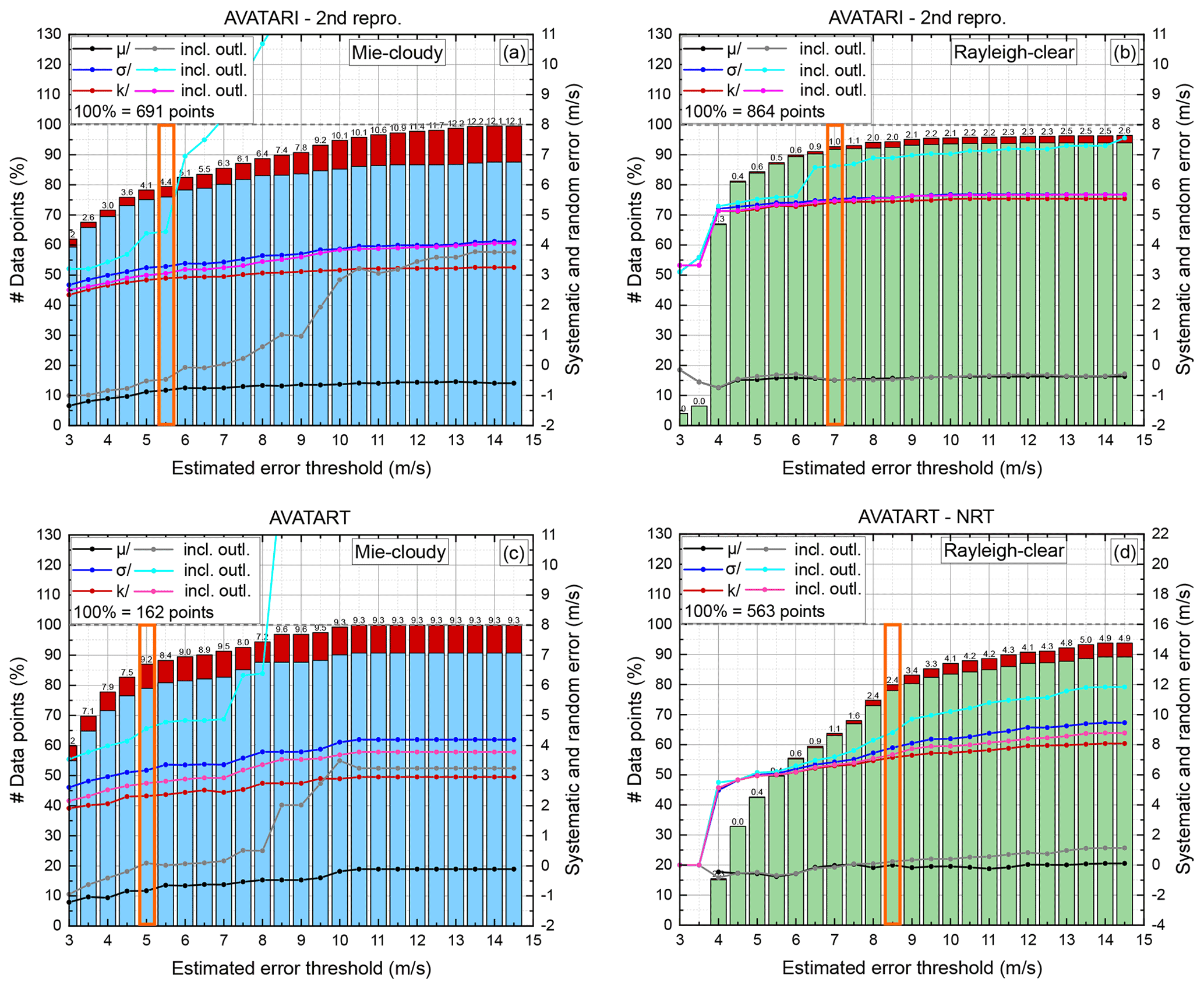
Figure 4Results from the statistical comparison of Aeolus L2B Mie-cloudy (a, c) and Rayleigh-clear winds (b, d) against 2 µm DWL data (one scan accumulation) are shown from the 10 underflights of the AVATAR-I campaign (a, b) and the 11 underflights of the AVATAR-T campaign (c, d), depending on the EE threshold without and with outlier removal based on the modified Z score. The bar plots depict the portion of filtered winds after QC (Zm<3, green and blue bars) and gross errors (Zm>3, red bars) from all wind results that are flagged as valid in the L2B product (left y axes). The percentage of gross errors is indicated above the bars. The lines and symbols refer to the statistical results (mean bias μ, standard deviation σ, and scaled MAD k) without removing the gross errors from the data sets (gray, light blue, magenta), while the black, blue, and red lines represent the statistical parameters after QC based on the modified Z score (right y axes). The EE thresholds that are deemed reasonable to provide robust statistical results are highlighted by orange frames.
As expected, the number of available valid data points increases when increasing the EE threshold. This is true for both Rayleigh-clear (green bars) and Mie-cloudy winds (blue bars) and for both campaign data sets. At the same time, the number of outliers in the data set also increases. Additionally, it can be seen that the mean bias (black without and gray with outliers), the standard deviation (dark blue without and light blue with outliers), and the scaled MAD (red without and magenta with outliers) are dependent on the EE threshold. This further demonstrates that the EE threshold can significantly impact the results of the statistical comparison.
In the following, several subjectively selected quality criteria are used to define a suitable EE threshold. For instance, it is checked for which EE threshold the SD starts to deviate from the scaled MAD, as this marks the point where the data set starts to deviate from a normal distribution. Furthermore, the number of available data points and determined outliers is analyzed. If too many outliers are determined, the QC can be considered too strict. Additionally, it is checked if the respective statistical quantities differ significantly when being calculated from the data set with and without outliers.
For the Rayleigh-clear winds of the AVATAR-I data set (Fig. 4b), for instance, the number of available data points increases quickly with increasing EE threshold. For an EE threshold of 4.5 m s−1, 80 % of all data points are already included, and only 0.4 % outliers are detected. Furthermore, for this threshold, the SD and the scaled MAD are almost similar for both cases calculated with and without outliers. Between an EE threshold of 6.0 and 6.5 m s−1, the SD calculated including outliers makes a jump of about 1 m s−1, whereas the other quantities remain rather constant. For an EE threshold larger than 7.0 m s−1, mainly outliers are added to the data set. Thus, 7.0 m s−1 is considered the optimum EE threshold for Rayleigh-clear winds of the AVATAR-I data set.
For the Rayleigh-clear winds of the AVATAR-T data set, which was acquired almost 2 years later in a different geographical region and at decreased ALADIN signal performance, the distribution looks different (Fig. 4d). The number of valid data points increases much slower compared to the AVATAR-I case. For an EE threshold of 7.0 m s−1, the SD is still rather close to the scaled MAD; however, only 65 % of the data points are included. By further increasing the EE threshold to 8.5 m s−1, the number of data points used increases to 78 %. For even larger EE thresholds, the difference of the scaled MAD calculated without (red) and with (magenta) outliers starts to increase, indicating that the outliers start to have an impact on the calculated statistical parameters. Thus, an EE threshold of 8.5 m s−1 seems to be a good compromise for the Rayleigh-clear winds of the AVATAR-T data set.
For the Mie-cloudy data set, the distribution of statistical parameters is even more sensitive to the EE threshold. It can be seen that Mie-cloudy winds in general contain more outliers. This also confirms that the QC by means of the validity flag and the EE threshold is not sufficient and that an additional QC by means of the modified Z score is needed, especially for the Mie-cloudy winds (Lux et al., 2022b). Following the same logic as for the Rayleigh-clear winds, an optimal EE threshold of 5.5 m s−1 is determined for the Mie-cloudy winds of the AVATAR-I data set and 5.0 m s−1 for the Mie-cloudy winds of the AVATAR-T data set. It is worth mentioning that the statistical comparison of AVATAR-T Mie-cloudy winds is not very sensitive to the actual EE threshold. For instance, an EE threshold of up to 7.0 m s−1 would yield similar results.
A scatter plot of Aeolus HLOS wind speeds versus 2 µm DWL data is shown in Fig. 5 for the AVATAR-I data set (left) as well as for the AVATAR-T data set (right). Rayleigh-clear winds and Mie-cloudy winds are indicated by blue dots and orange dots, respectively, and corresponding line fits are depicted by the light blue and yellow lines. The x=y line is represented by the gray dashed line.
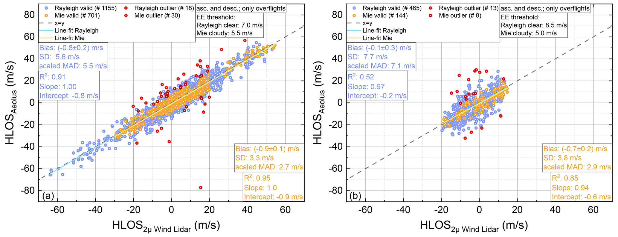
Figure 5Aeolus HLOS wind speed plotted against the 2 µm DWL wind speed, projected onto the horizontal viewing direction of Aeolus for the 10 underflights performed during the AVATAR-I campaign (left) and for the 11 underflights performed during the AVATAR-T campaign (right). The wind measurements are separated into Rayleigh-clear winds (blue) and Mie-cloudy winds (orange). Outliers that exceeded a modified Z-score threshold of 3 are indicated by light red and dark red points, respectively. Corresponding least-square line fits are indicated by the light-blue and yellow line, respectively. The fit results are shown in the insets. The x=y-line is represented by the gray dashed line.
Altogether, the 10 underflights during the AVATAR-I campaign provide 1155 valid data points for Rayleigh-clear wind validation and 701 valid data points for Mie-cloudy wind validation. The QC identified 18 (1.6 %) data points of the Rayleigh-clear data set and 30 (4.3 %) data points of the Mie-cloudy data set as outliers, as they exceeded the modified Z-score threshold of 3 according to Eq. (8). The 11 underflights during AVATAR-T resulted in 465 and 144 data points for Rayleigh-clear and Mie-cloudy wind validation, respectively, where the modified Z-score threshold led to the identification of 13 (2.8 %) and 8 (5.6 %) outliers. The decreased number of data points observed during the last six AVATAR-T underflights (for detailed itemization see Table 2) was due to the fact that the 2 µm DWL was degrading during the campaign period. The degradation itself was caused by the large temperature and humidity gradients causing the transceiver unit to get misaligned. It is worth mentioning here that, due to the heterodyne-detection measurement principle of the 2 µm DWL, the progressive misalignment only led to a reduction in the data coverage but not to an increase in the systematic or random error of the wind observations over the course of the mission. Furthermore, the Aeolus RBS (see also Fig. 2), with thicker but fewer range gates in the troposphere for the sake of increased SNR, was less favorable for a good grid overlap with airborne data which are only acquired from flight altitudes of about 10 km a.m.s.l. down to the ground. Additionally, the overall signal levels during the AVATAR-T period were only about half of the one acquired during AVATAR-I, caused by a degrading Aeolus instrument performance.
5.1 Systematic error
The mean systematic error of the Aeolus wind data and its corresponding uncertainty are calculated according to Eqs. (3) and (6), respectively. It yields values of m s−1 (Rayleigh-clear) and m s−1 (Mie-cloudy) for the AVATAR-I data set and m s−1 (Rayleigh-clear) and m s−1 (Mie-cloudy) for the AVATAR-T data set, respectively. Hence, the systematic errors for both wind products and both campaign periods are close to the specified mission requirement of 0.7 m s−1 for Aeolus HLOS winds (ESA, 2016). Compared to the previous campaign results where the systematic error was determined to be (2.1±0.3) m s−1 (Rayleigh-clear) and (2.3±0.2) m s−1 (Mie-cloudy) for the WindVal III data set and m s−1 (Rayleigh-clear) and m s−1 (Mie-cloudy) for AVATAR-E, a significant decrease in the systematic error can be observed (see also Table 3), which is due to the implementation of correction schemes for the hot pixels and the thermal fluctuations on the telescope mirror in the Aeolus processor that were not available in the early phase of the mission. It is worth mentioning that, for the analysis of the AVATAR-I campaign, which was performed in fall 2019, the second reprocessed Aeolus data set is used (B11) and hence also contains the correction scheme for the telescope temperature fluctuations. The Aeolus processor versions used for the analysis of the respective campaign data sets are also given in Table 3. Furthermore it has to be pointed out the results from the different campaign data sets are not necessarily comparable, as they are dependent on the applied QC procedure, as discussed in Sect. 4.3.
5.2 Random error
The random error of the Aeolus wind is represented by the scaled MAD according to Eq. (5). It is determined to be 5.5 m s−1 (Rayleigh-clear) and 2.7 m s−1 (Mie-cloudy) for the AVATAR-I data set and 7.1 m s−1 (Rayleigh-clear) and 2.9 m s−1 (Mie-cloudy) for the AVATAR-T. The impact of the 2 µm DWL uncertainty of about 1 m s−1 (see also Witschas et al., 2020) on the determined random error is only marginal. It can be recognized that the mean random error of Rayleigh-clear winds is significantly larger than the 2.5 m s−1 originally specified for Aeolus HLOS winds at altitudes between 2 and 16 km (ESA, 2016; Kanitz et al., 2019; Reitebuch et al., 2020). The main reason for this is the lower signal levels of the backscattered light from the atmosphere, which are indicated to be caused by a combination of instrumental misalignment, the wavefront error of the 1.5 m telescope, and laser-induced contamination (LIC) within the system.
Furthermore, it can be seen that the Rayleigh-clear random error increased by about 30 % between the AVATAR-I and the AVATAR-T campaigns, although the actual laser UV energy was 20 % larger during the AVATAR-T campaign. However, the atmospheric signal level itself was about 50 % smaller due to the aforementioned degradation. This signal decrease was partly compensated for by enlarging the Aeolus range bins during the AVATAR-T campaign, which were 750 m instead of 500 m, as applied during AVATAR-I. Additionally, the solar background signal was smaller by about a factor of 3 during AVATAR-T, which also partly compensates for the overall signal decrease. The mean useful signal – which denotes the average signal level per observation in LSB (least significant bit) after being corrected for the detection chain offset (DCO), the solar background, and the dark current – is determined to be (247±1) LSB for Rayleigh signals during AVATAR-I and (175±3) LSB for AVATAR-T. Considering just Poisson noise in the measured data set, the random error can be considered to be proportional to , where N is the signal level. Hence, by using the random error determined from AVATAR-I and considering the mean useful signal levels of both campaign data sets, the random error for AVATAR-T would be expected to be m s−1, which is close to the measured value of 7.1 m s−1. It should also be mentioned that the error calculation based on signal levels is only a rough approximation, as valid Rayleigh-clear winds are also available in aerosol-loaded areas with a scattering ratio larger than 2 or 3. Hence, the signal does not necessarily originate from backscattering on molecules, which would distort the random error calculation of the Rayleigh-clear winds.
Table 3Aeolus systematic and random error determined from different campaign data sets.

* Values taken from (Witschas et al., 2020).
5.3 Falcon in situ measurements
In addition to 2 µm DWL observations, in situ measurements performed on board the Falcon aircraft were statistically analyzed, as demonstrated by the scatter plot shown in Fig. 6. Here, the Aeolus HLOS Rayleigh-clear wind speeds are plotted versus Falcon in situ data for the AVATAR-I data set (blue dots) as well as for the AVATAR-T data set (green dots). Line fits to the data are depicted by the dark blue and green lines, and the x=y line is represented by the gray dashed line. The Falcon measurements are mainly taken at altitudes between 10 and 11 km and have a random error of 0.9 m s−1, with a temporal resolution of 1 s, hence providing very good reference data. It is only the representativeness error that is difficult to assess, as it is dependent on the vertical homogeneity of the atmosphere in the vicinity of the performed observations. Furthermore, as no Mie-cloudy winds were present at flight level, only Rayleigh-clear winds could be analyzed.
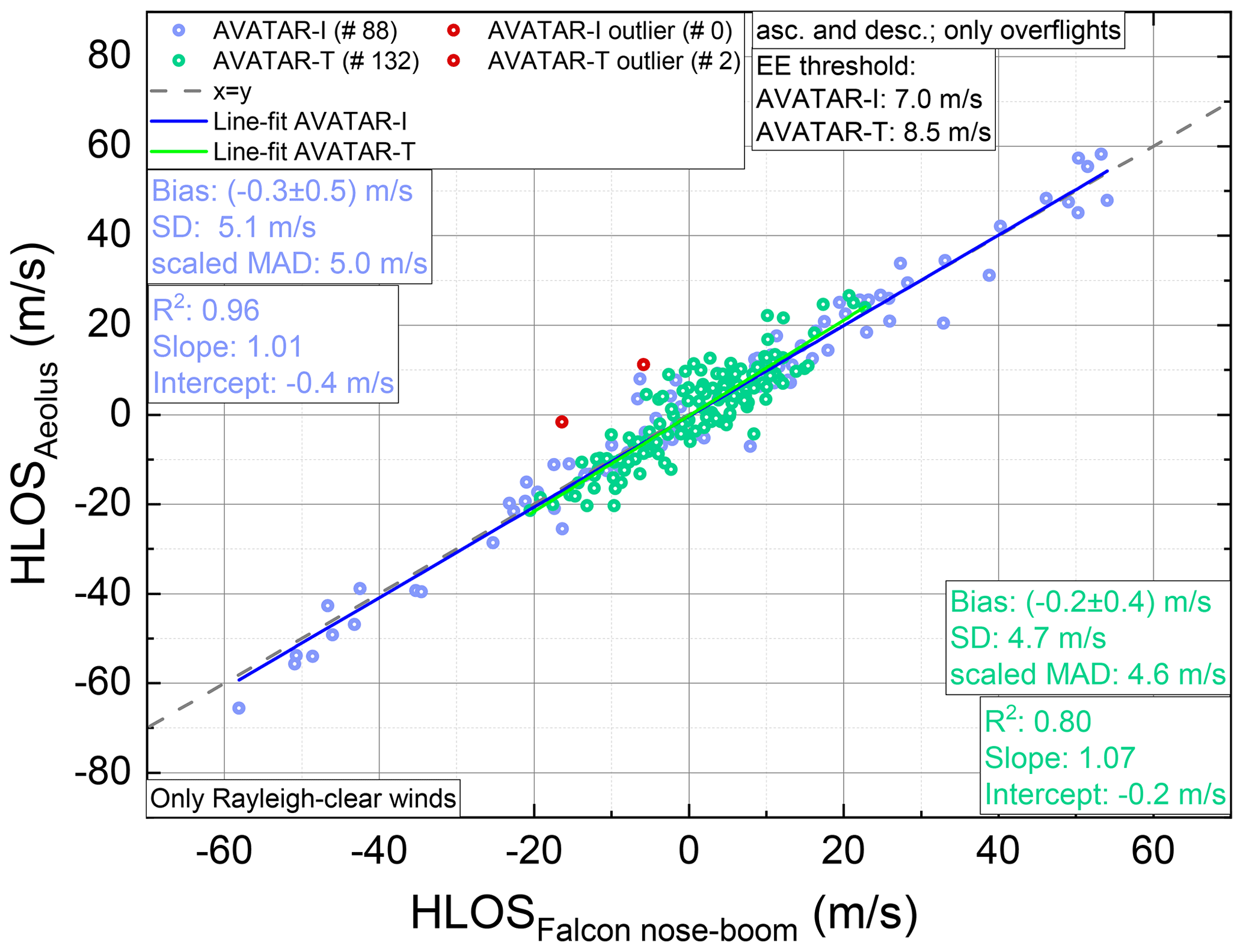
Figure 6Aeolus Rayleigh-clear HLOS winds plotted against the Falcon nose boom wind speed projected onto the horizontal viewing direction of Aeolus for the 10 underflights performed during the AVATAR-I campaign (blue) and for the 11 underflights performed during the AVATAR-T campaign (green). Outliers that exceeded a modified Z-score threshold of 3 are indicated by light red and dark red points, respectively. Corresponding least-square line fits are indicated by the dark blue and light green line, respectively. The fit results are shown in the insets. The x=y-line is represented by the gray dashed line.
The mean systematic error is determined to be m s−1 (AVATAR-I) and m s−1 (AVATAR-T) and hence confirms the results obtained from the 2 µm DWL analysis and that the Aeolus Rayleigh-clear winds meet the mission requirement of a systematic error smaller than 0.7 m s−1.
The corresponding random errors yield values of 5.0 m s−1 (AVATAR-I) and 4.6 m s−1 (AVATAR-T). Thus, for the AVATAR-I data set, the random error is comparable to the one determined from the 2 µm DWL (5.5 m s−1) but differs significantly for the AVATAR-T data set, where the 2 µm DWL analysis yields a random error of 7.1 m s−1. This is explained by the fact that the Rayleigh-clear random error depends on the signal level, which is lower at lower altitudes (see also Sect. 6). For the AVATAR-T campaign, lower signal levels in the SAL due to the extinction induced by aerosols cause the random error of Rayleigh-clear winds to increase in this region. Hence, the mean random error is larger in lower altitudes compared to the one at flight level.
In Sects. 5.1 and 5.2, the mean systematic and random error was determined for the entire data sets of the AVATAR-I and the AVATAR-T campaigns and for both Rayleigh-clear and Mie-cloudy winds. In this section, the dependency of these errors on the actual wind speed, represented by the 2 µm DWL observations, is investigated to verify if the Aeolus calibration routine works for the entire wind speed range. Moreover, the error dependency on the geographical location is investigated. To study the representativity of the comparison between the 2 µm DWL observations, which may have a temporal distance to the Aeolus overflight of up to 1 h, the error dependency on the time difference between 2 µm DWL observations and the Aeolus overflight is analyzed. Further, it is verified whether the error has any dependency on the scattering ratio, which might be induced by a cross-talk between the signals from the Rayleigh and the Mie channels, respectively. It has to be mentioned that the Aeolus scattering ratio data are still preliminary and subject to processor improvements. For instance, for the AVATAR-I data set, the scattering ratio values were taken from the L2B data. For the AVATAR-T data set, however, scattering ratio values were partly set to 1 to avoid problems with the assimilation of Aeolus data in the ECMWF model. Hence, the scattering ratio values were calculated from L1B after adaptation to the L2B grid and averaging, as it was done for the wind processing. Furthermore, it has to be pointed out that the scattering ratio values retrieved for Rayleigh-clear winds in broken-cloud conditions could be faulty due to grouping issues that appear when going from L1B to L2B data. Thus, especially for Rayleigh-clear winds, no solid conclusions can be drawn from scattering ratio data. Nevertheless, the data are shown to represent the current status of the Aeolus data processor. In addition to that, the mean useful signal, the EE, the scattering ratio, and the actual wind speed are analyzed depending on altitude. These analyses are separated into Rayleigh-clear winds (Sect. 6.1) and Mie-cloudy winds (Sect. 6.2) and provide further insights into the Aeolus error characteristics.
6.1 Rayleigh-clear winds
In Fig. 7, the dependency of the Aeolus Rayleigh-clear HLOS wind speed error with respect to the 2 µm DWL (Eq. 2) on the 2 µm DWL-measured wind speed (a), on the latitude (b), on the time difference between Aeolus and 2 µm DWL observation (c), and on scattering ratio (d) is shown. The data from AVATAR-I are indicated in blue and from AVATAR-T in orange. The solid lines denote the median value for certain intervals, and the shaded area represents the median plus–minus the scaled MAD. To have enough data points and hence a reliable value for the mean and the scaled MAD, the averaging intervals Δ for the AVATAR-I and AVATAR-T data sets are chosen to be Δ=(5.8 and 1.7) m s−1 (2 µm DWL wind speed), (latitude), Δ=(296 and 342) s (time difference), and Δ=0.95 and 0.98 (scattering ratio), respectively.
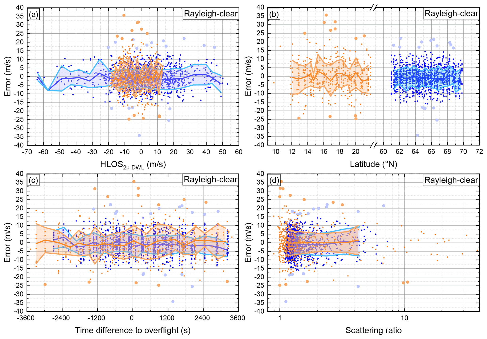
Figure 7Aeolus Rayleigh-clear HLOS wind speed error with respect to 2 µm DWL measurements depending on 2 µm DWL-measured wind speed (a), on latitude (b), on time difference between Aeolus and 2 µm DWL observation (c), and on scattering ratio (d). The data set of the AVATAR-I campaign is indicated in blue and the one of AVATAR-T in orange. The solid lines denote the median value for certain intervals, and the shaded area represents the median plus–minus the scaled MAD. Large dots represent outliers which were identified by modified Z score with a threshold of 3 that is calculated for the respective averaging interval.
From Fig. 7a, it is obvious that the Aeolus wind speed error has no significant dependency on the actual wind speed which is represented by the 2 µm DWL. Both the median (systematic error) and the scaled MAD (random error) are nearly constant for all wind speeds and both campaign data sets. Please note that the median is used instead of the mean to be insensitive to single outliers of the small number of data for each averaging interval. Still, single outliers for very high wind speeds during the AVATAR-I campaign are an artifact caused by a lack of sufficient data points. Furthermore, especially for the AVATAR-I data set, it is evident that there are more outliers with a positive error than with a negative one. A potential explanation for this behavior is not available so far.
In Fig. 7b, the error is plotted against the latitude. As both campaign sites were at different latitudes, the x axis has a break between 22 and 59∘ N, but both sides cover the same range of 13∘. As for the wind speed, no significant dependency of the systematic and random error on the latitude can be recognized. It is probable that the usual range covered during Falcon campaigns (≈10∘) is not enough to resolve any geolocation dependency of the Aeolus errors.
In addition, it is investigated whether the time difference between the Aeolus overpass and the actual 2 µm DWL observation on the track has an impact on the determined wind speed error (Fig. 7c). It can be seen that the maximum temporal discrepancy between the Aeolus overpass and the 2 µm DWL observation is always smaller than 1 h and that neither the systematic nor the random error is significantly dependent on this time difference.
The dependency of the Aeolus errors on the scattering ratio is shown in Fig. 7d. It is obvious that Rayleigh-clear winds are even available for scattering ratios of 10 and larger. However, as mentioned before, it cannot be guaranteed that the scattering ratio data represent the actual atmospheric composition of the volume from which the Rayleigh-clear wind was retrieved. Still, for the given data, no dependency of the systematic error on the scattering ratio can be observed. In addition, it can be seen that outliers, determined by the modified Z-score threshold of 3, appear for low as well as for high backscatter ratios.
Hence, the Aeolus mean systematic and random errors are neither significantly dependent on the wind speed nor on the latitude, the time difference, and the scattering ratio, confirming that the Aeolus calibration is working properly. It has to be mentioned that these results are restricted to certain geographical regions, certain time periods, and a limited number of data points. Thus, it is probable that not all error contributions can be detected in this analysis, especially if those are related to strong non-periodic sources like strong deviations from the atmospheric temperature profile or orbital variations. For an even more conclusive error characterization, data from other CalVal teams as well as model data are needed.
In Fig. 8, the altitude dependency of the mean useful signal (a), the estimated error (b), the Aeolus error with respect to the 2 µm DWL observations (c), the scattering ratio (d), and the HLOS wind velocity derived from 2 µm DWL measurements (e) for Rayleigh-clear wind observations available for the AVATAR-I data set (blue) and the AVATAR-T data set (orange) is shown. The mean useful signal denotes the mean signal level per observation and the range bin in LSB after being corrected for the detection DCO, the solar background, and the dark current. The actual valid data points are indicated by the small dots, and corresponding outliers, defined by a modified Z-score threshold of 3, are plotted by larger dots. The median value per each range gate is indicated by the solid line, and the shaded area indicates the median plus–minus the scaled MAD for each range bin.
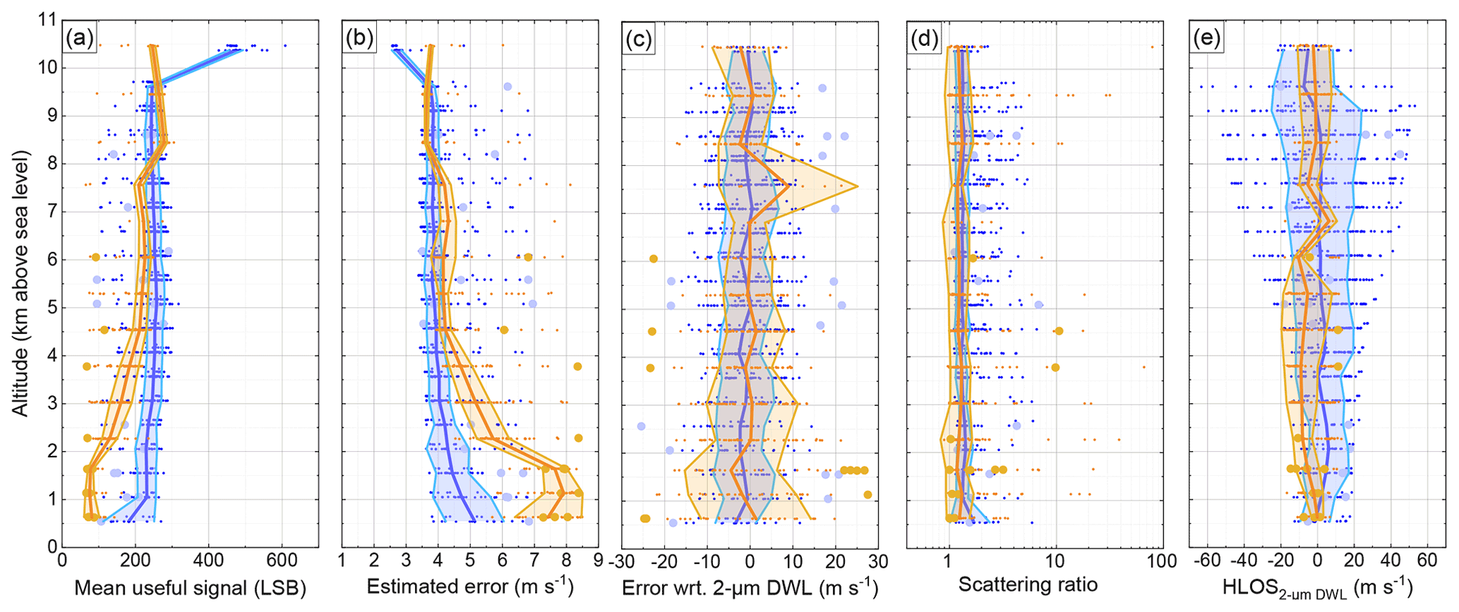
Figure 8Altitude dependency of the mean useful signal (a), the estimated error (b), the Aeolus error with respect to the 2 µm DWL observations (c), the scattering ratio (d), and the HLOS wind velocity derived from 2 µm DWL measurements (e) for Rayleigh-clear wind observations available for the AVATAR-I data set (blue) and the AVATAR-T data set (orange). The actual valid data set is indicated by the small points; the outliers defined by the modified Z-score threshold of 3 are plotted by larger dots. The median value per each range gate is indicated by the solid line, and the shaded area indicates the median plus–minus the scaled MAD for each range gate.
By analyzing the altitude dependency of the mean useful signal (Fig. 8a), it can be seen that the two data sets differ. For AVATAR-I (blue), the signal levels are rather constant at about 240 LSB. Only at altitudes of about 10.5 km is the signal level twice as high due to the larger range bin size at this altitude (see also Fig. 2). On the contrary, the mean signal level for the AVATAR-T data shows a remarkable decrease between about 4.5 km and the ground, which is due to the signal extinction caused by the aerosols that are prominent in the SAL. Even at altitudes above 4.5 km, the signal levels for AVATAR-T data were lower than for AVATAR-I, although the range bins were already increased to 750 m. This additionally confirms that the decreasing Aeolus performance leads to lower (Rayleigh-clear) signal levels at all altitudes. Furthermore, it can be observed that outliers appear in all altitudes and were successfully determined by the applied Z-score threshold.
The altitude dependency of the EE is plotted in Fig. 8b. It can be seen that it is indirectly proportional to the signal levels shown in panel (a). All regions of smaller signal levels correspond to a larger EE (as expected). For AVATAR-I, the EE is about 4 m s−1 at all altitudes, except for the highest range bin at about 10.5 km, where it goes down to 2.5 m s−1 due to the larger range bin size. At lower altitudes, it goes up to 5 m s−1 due to the lower signal levels in this region. For the AVATAR-T data set, the EE is about 4 to 4.5 m s−1 between 4.5 and 10.5 km altitude and increases up to 7.5 m s−1 below due the low signal levels in this region. This also explains why the random error retrieved from the Falcon observations at about 10.5 km altitude (5.0 m s−1) is significantly lower than the mean random error derived from all 2 µm DWL observations (7.1 m s−1).
In Fig. 8c, the Aeolus error with respect to the 2 µm DWL is shown. It can be observed that the mean bias does not show any height dependency for both data sets. The outlier at 7.5 km of the AVATAR-T data set is a result of an insufficient number of data points. Furthermore, it can be seen that the random error follows the EE (Fig. 8b) rather well. In particular, the random error increase for AVATAR-T in the SAL is predicted well by the EE.
The height dependency of the scattering ratio is depicted in Fig. 8d. It can be realized that Rayleigh-clear winds are available even for scattering ratios up to 10 and larger and that these scattering ratios occur at all altitudes. However, as mentioned above, these data have to be treated with caution. The mean scattering ratio is below 1.5 for both data sets and all altitudes.
In Fig. 8e, the 2 µm DWL winds are shown to be range resolved, demonstrating that much higher wind speeds between −60 and 55 m s−1 were measured during AVATAR-I (blue) and mainly at altitudes between 6 and 10 km in the vicinity of the North Atlantic jet stream. During AVATAR-T, the measured wind speeds were much lower, varying between −20 and 18 m s−1, and had their maximum between 3 and 6 km, which is most probably related to the African easterly jet.
6.2 Mie-cloudy winds
A similar analysis as shown for Rayleigh-clear winds in Fig. 7 is done for Mie-cloudy winds, as presented in Fig. 9. Since fewer data points are available for Mie-cloudy winds, the averaging intervals Δ for the AVATAR-I and AVATAR-T data sets had to be enlarged to Δ=(10.5 and 4.3) m s−1 (2 µm DWL wind speed), Δ=(1.2 and 1.6)∘ (latitude), Δ=(604 and 677) s (time difference), and Δ=6.9 and 7.4 (scattering ratio), respectively.
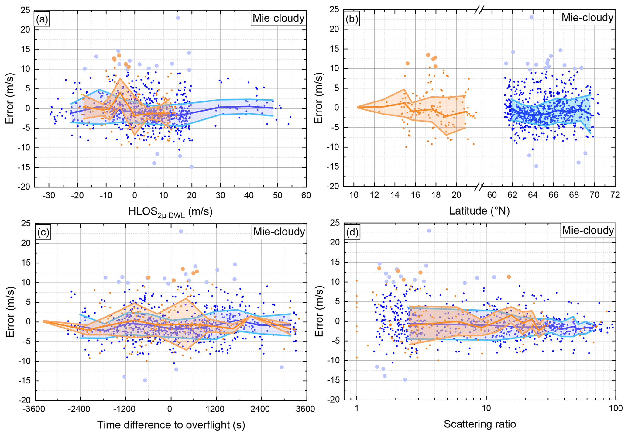
Figure 9Aeolus Mie-cloudy HLOS wind speed error with respect to 2 µm DWL measurements depending on 2 µm DWL-measured wind speed (a), on latitude (b), on the time difference between Aeolus and 2 µm DWL observation (c), and on the scattering ratio (d). The data set of the AVATAR-I campaign is indicated in blue, and the one of AVATAR-T in orange. The solid lines denote the median value for certain intervals; the shaded areas represent the median ± scaled MAD. Large dots represent outliers which were identified by modified Z score with a threshold of 3 that is calculated for the respective averaging interval.
The dependency of the Aeolus wind error on the actual wind speed represented by the 2 µm DWL is shown in Fig. 9a. For the AVATAR-I data set, it can be recognized that there are regions where the error is negative – as, for instance, for a 2 µm DWL-measured wind speed around 15 m s−1, where the systematic error is about −2 m s−1. As this is also the region with the most data points, this explains the overall negative systematic error of −0.9 m s−1 retrieved from the statistical comparison. Furthermore, it can be seen that there are remarkably more outliers towards positive errors. This was already true for Rayleigh-clear winds; however, it cannot be concluded that this is due to the same root cause, which is essentially unknown and a topic for further investigations.
The dependency of the Aeolus Mie-cloudy wind speed error on latitude is indicated in Fig. 9b. For the AVATAR-I data set (blue), it can be seen that the median is negative for all latitudes, varying between 0 and −2 m s−1. The modulation of the median is not meaningful due to a lack of sufficient data points. This is even more true for the AVATAR-T data set, where no conclusion can be drawn from the latitude-averaged data set.
In Fig. 9c, the Aeolus Mie-cloudy error is plotted with respect to the time difference between Aeolus overpass and 2 µm DWL observation. As for the Rayleigh-clear winds, no significant dependency can be observed for either data set. Thus, even Mie-cloudy winds seem to change only marginally within a ±1 h timeframe (on average), although Mie-cloudy winds are expected to have a higher variability compared to Rayleigh-clear winds.
Fig. 9d depicts the Aeolus error depending on the scattering ratio. From the AVATAR-I data set, it can be seen that the scattering ratio extends to values of up to 100 and that the median drifts to negative values for larger scattering ratios. Also, the random error is significantly reduced from about m s−1 for lower scattering ratios (0–10) to m s−1 for larger backscattering ratios (20–100). Hence, it can be concluded that the accuracy and precision of Mie-cloudy winds are dependent on the scattering ratio. In particular, observations with a higher backscatter ratio and, thus, a better SNR provide more accurate Mie-cloudy winds; however, they also present a different bias, a topic which has to be investigated in the future. A similar behavior can be seen from the AVATAR-T data set, although it is less conclusive due to the lower number of available data points.
Furthermore, similar to the Rayleigh-clear wind analysis, the altitude dependency of the mean useful signal (a), the estimated error (b), the Aeolus error with respect to the 2 µm DWL observations (c), the scattering ratio (d), and the HLOS wind velocity derived from 2 µm DWL measurements (e) is investigated for Mie-cloudy winds from the AVATAR-I data set (blue) and the AVATAR-T data set (orange), as shown in Fig. 10.
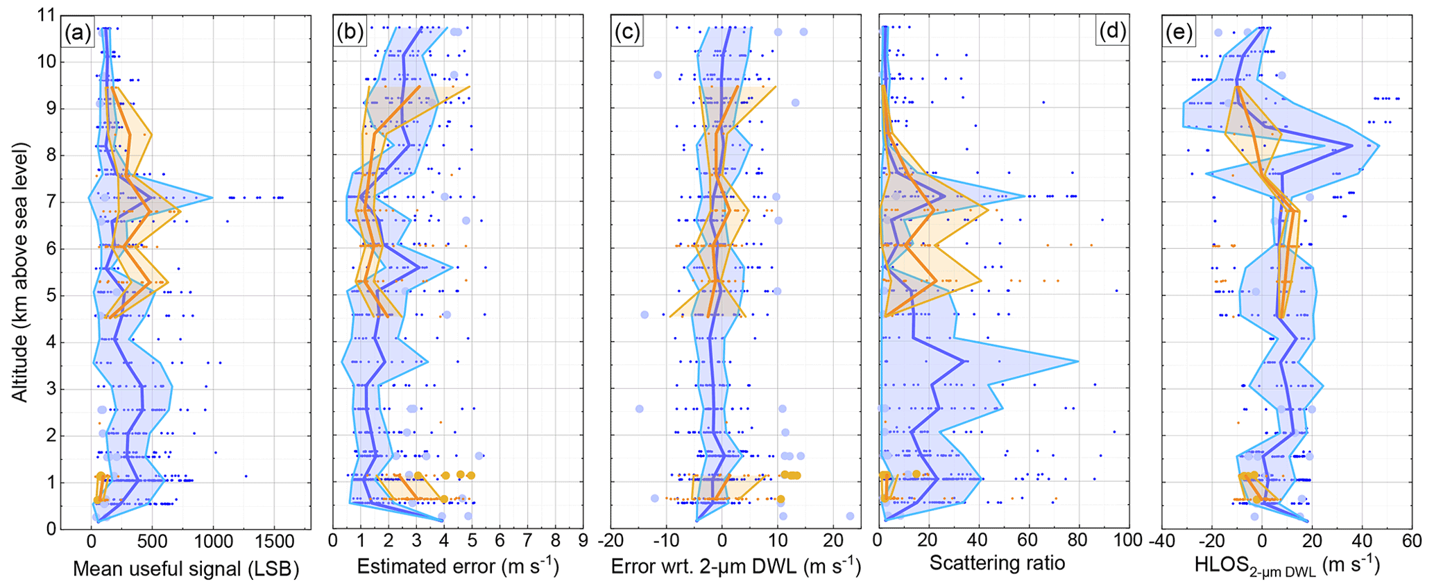
Figure 10Dependency of the mean useful signal (a), the estimated error (b), the Aeolus error with respect to the 2 µm DWL observations (c), the scattering ratio (d), and the HLOS wind velocity derived from 2 µm DWL measurements (e) for Mie-cloudy wind observations available for the AVATAR-I data set (blue) and the AVATAR-T data set (orange). The actual valid data set is indicated by the small points; the outliers defined by the modified Z-score threshold of 3 are plotted by larger dots. The median value per each range gate is indicated by the solid line, and the shaded area indicates the median plus–minus the scaled MAD for each range gate.
From Fig.10a, it can be seen that the mean useful signal varies much more than for Rayleigh-clear winds from almost 0 up to about 1600 LSB for the AVATAR-I data set at about 7 km altitude. The mean signal levels range from about 100 to 500 LSB for both data sets. Furthermore, it is interesting to realize that no Mie-cloudy winds are available for the AVATAR-T data set between 1 and 4.5 km altitude, which represents the dust-laden SAL. Thus, Mie-cloudy winds are indeed just retrieved from cloud returns and not from aerosol-rich regions. This is a known issue and is related to the scattering ratio thresholds and grouping schemes that are currently used in the Aeolus processor. Outliers appear in all altitudes but mainly for low signal levels.
The altitude-dependent EE is depicted in Fig. 10b. In general, as for Rayleigh-clear winds, the EE is smaller in regions of larger signal levels. However, as the Mie-cloudy EE does not directly depend on the signal level but on the accuracy of the actual fit routine, this behavior is less pronounced. The mean EE ranges from about 1 to 3 m s−1 for both data sets.
The altitude-dependent Aeolus error with respect to the 2 µm DWL observations is shown in Fig. 10c. From the AVATAR-I data, it can be seen that the mean error is obviously negative ( m s−1) for altitudes between 4.5 km and the ground, where the random error is relatively small. This is also the region with larger scattering ratios, as they are shown in Fig. 10d, and thus confirms that the accuracy and precision of Mie-cloudy winds depend on the scattering ratio (see also Fig. 9d). The AVATAR-T data set does not provide enough data points to draw a similar conclusion. The scattering ratio, in general, varies from close to 1 up to 100, whereas the mean scattering ratio varies from close to 1 up to 30 for both data sets. For the AVATAR-I data set, larger scattering ratio values up to 30 are prominent at altitudes from the ground up to 4.5 km, which is also the region that shows an enhanced negative systematic error.
The altitude dependency of the measured 2 µm DWL winds is shown in Fig. 10e. The wind speed range is much smaller than for Rayleigh-clear winds and varies from about −30 to 50 m s−1 for AVATAR-I and from about −20 to 15 m s−1 for AVATAR-T. As for Rayleigh-clear winds, the highest wind speeds are found in the vicinity of the jet stream in the AVATAR-I data set.
In the past 3 years, DLR strongly contributed to Aeolus CalVal activities by means of airborne wind lidar measurements. In this study, the data quality of Aeolus L2B wind products in two regions of particular interest to NWP, namely the North Atlantic jet stream region and the region of tropical winds affected by dust transport from the Sahara, is analyzed. This analysis is based on airborne wind lidar data acquired from DLR's Falcon aircraft during two airborne campaigns performed in Iceland (AVATAR-I) and Cape Verde (AVATAR-T). During the AVATAR-I campaign, conducted from Keflavik, Iceland, in September 2019, 10 satellite underflights on ascending and, for the first time, descending orbits were performed. During the AVATAR-T campaign, conducted from Sal, Cape Verde, in September 2021, 11 satellite underflights on ascending and descending orbits were executed. In total, these underflights lead to about 19 000 km along the Aeolus measurement track that is used for comparison.
Based on a statistical analysis, the systematic and random errors of Aeolus HLOS wind observations are determined by comparison to 2 µm DWL observations. The 2 µm DWL is suitable as a reference instrument due to the low systematic and random errors that come along with the heterodyne-detection measurement principle of the system. This way, reliable values for the systematic and random errors for the AVATAR-I data set are determined to be and 5.5 m s−1 for Rayleigh-clear winds and and 2.7 m s−1 for Mie-cloudy winds, respectively. For the AVATAR-T data set, the systematic and random errors are and 7.1 m s−1 for Rayleigh-clear winds and and 2.9 m s−1 for Mie-cloudy winds, respectively. Thus, within the given uncertainty, the systematic error fulfills the requirement of being below 0.7 m s−1 for both wind products and both campaign data sets. This confirms the successful correction schemes for systematic errors that have been identified in the early phase of the mission. Hot pixels and the thermal variations on the Aeolus telescope mirror are treated in the refined Aeolus data processor after the release of the processor baseline 10 and following. The random error of Rayleigh-clear winds is significantly larger than specified (2.5 m s−1), which is due to the overall lower signal levels most likely caused by a combination of instrumental misalignment, the wavefront error of the 1.5 m telescope, and laser-induced contamination. The random error of Mie-cloudy winds is close to the specifications.
The results are confirmed by comparison against in situ data from the Falcon nose boom, which yield a systematic and random error for Rayleigh-clear winds of and 5.0 m s−1 for the AVATAR-I data set and and 4.6 m s−1 for the AVATAR-T data set. The lower random error compared to the 2 µm DWL analysis determined for the AVATAR-T data is shown to be due to the altitude dependency of the random error, which is caused by the height dependency of the signal levels, especially in aerosol-laden regions.
A detailed analysis of the Rayleigh-clear wind errors reveals that they are not significantly dependent on the actual wind speed nor on the geolocation (latitude), the time difference between 2 µm DWL observation and satellite overflight, and also not on the scattering ratio, which further confirms a proper calibration scheme of the Aeolus instrument. Moreover, based on an altitude-dependent analysis of the Aeolus wind speed error, it is shown that the random error mainly depends on the signal levels and that it is well represented by the estimated error, assuming that a proper quality control of Aeolus data by means of appropriate EE thresholds together with an additional Z-score-based outlier removal is performed in advance.
The detailed analysis of Mie-cloudy wind errors demonstrated that they are also not dependent on the actual wind speed, the geolocation (latitude), or the time difference between 2 µm DWL observation and satellite overflight, but showed a dependence on the scattering ratio. In particular, the systematic error drifts to more negative values, and the random error is reduced for larger scattering ratios. This is also confirmed by the altitude-dependent analysis that shows larger negative systematic errors at altitudes where the scattering ratio is enhanced. Furthermore, it is revealed that Mie winds are indeed only available from cloudy returns. Aerosol-laden regions such as the SAL only provide Rayleigh-clear and no Mie winds.
This analysis is an important contribution to evaluating the quality of Aeolus winds and the fulfillment of mission requirements defined in advance. It shows that Aeolus (almost) fulfills the required values that were originally specified. The larger random errors are due to the lower signal levels that are caused by a combination of initial misalignment and laser-induced contamination.
The code that is used for data analysis (Labview) and figure plotting (Origin Lab) can be provided upon request.
The presented work includes data from the Aeolus mission, which is part of the European Space Agency (ESA) Earth Explorer Programme. This includes the second reprocessed L2B wind product (Baseline 11) for the period of the AVATAR-I campaign (from 9 September through 1 October 2019) and the NRT L2B wind product (Baseline 12; https://earth.esa.int/eogateway/documents/20142/37627/Aeolus-L2B-2C-Input-Output-DD-ICD.pdf, last access: 5 December 2022; de Kloe et al., 2022) for the period of the AVATAR-T campaign (from 6 through 28 September 2021), which are both publicly available and accessible via the ESA Aeolus Online Dissemination System (https://aeolus-ds.eo.esa.int/oads/access/collection/L2B_Wind_Products, last access: 5 December 2022; ESA, 2022). The processor development, improvement, and product reprocessing preparation have been performed by the Aeolus DISC (Data, Innovation and Science Cluster), which involves DLR, DoRIT, TROPOS, ECMWF, KNMI, CNRS, S&T, ABB, and Serco, in close cooperation with the Aeolus PDGS (Payload Data Ground Segment). The 2 µm DWL data used in this paper can be provided upon reasonable request to Benjamin Witschas (benjamin.witschas@dlr.de).
BW prepared the main part of the paper and performed the corresponding analyses. SR performed the 2 µm DWL data analysis. CL, OL, and UM provided A2D data for further comparison and helped with the preparation of the paper. AG and AS performed the weather forecast during the campaigns, provided meteorological data for the data analyses, and helped with the preparation of the paper. FW provided the original and reprocessed Aeolus data that are used within this study. OR helped with the data analyses and the preparation of the paper.
The contact author has declared that none of the authors has any competing interests.
Publisher's note: Copernicus Publications remains neutral with regard to jurisdictional claims in published maps and institutional affiliations.
This article is part of the special issue “Aeolus data and their application (AMT/ACP/WCD inter-journal SI)”. It is not associated with a conference.
The presented work includes preliminary data (not fully calibrated or validated and not yet publicly released) of the Aeolus mission that is part of the European Space Agency (ESA) Earth Explorer Programme. The processor development, improvement, and product reprocessing preparation are performed by the Aeolus DISC (Data, Innovation and Science Cluster), which involves DLR, DoRIT, ECMWF, KNMI, CNRS, S&T, ABB, and Serco in close cooperation with the Aeolus PDGS (Payload Data Ground Segment). The analysis has been performed in the framework of the Aeolus Data Innovation and Science Cluster (Aeolus DISC). We are grateful to our ESA colleagues, Thorsten Fehr (Aeolus scientific campaign coordinator) and Jonas von Bismarck (Aeolus data quality manager), for their support of the study. Moreover, we would like to thank the DLR flight experiments department for the realization of the AVATAR-T airborne campaign despite the obstacles posed by the COVID-19 pandemic.
This research has been supported by the Deutsches Zentrum für Luft- und Raumfahrt (ADM-III Verlängerung grant), the European Space Agency (grant nos. 4000128136/19/NL/IA and 4000129946/20/NL/IA), and the German Federal Ministry for Economic Affairs and Energy (BMWi, grant no. 50EE1721A).
The article processing charges for this open-access publication were covered by the German Aerospace Center (DLR).
This paper was edited by Ad Stoffelen and reviewed by Thomas Flament and one anonymous referee.
Ansmann, A., Wandinger, U., Le Rille, O., Lajas, D., and Straume, A.: Particle backscatter and extinction profiling with the spaceborne high-spectral-resolution Doppler lidar ALADIN: methodology and simulations, Appl. Opt., 46, 6606–6622, 2007. a
Baars, H., Herzog, A., Heese, B., Ohneiser, K., Hanbuch, K., Hofer, J., Yin, Z., Engelmann, R., and Wandinger, U.: Validation of Aeolus wind products above the Atlantic Ocean, Atmos. Meas. Tech., 13, 6007–6024, https://doi.org/10.5194/amt-13-6007-2020, 2020. a, b, c
Baker, W. E., Atlas, R., Cardinali, C., Clement, A., Emmitt, G. D., Gentry, B. M., Hardesty, R. M., Källén, E., Kavaya, M. J., Langland, R., Ma, Z., Masutani, M., McCarty, W., Pierce, R. B., Pu, Z., Riishojgaard, L. P., Ryan, J., Tucker, S., Weissmann, M., and Yoe, J. G.: Lidar-Measured Wind Profiles: The Missing Link in the Global Observing System, B. Am. Meteorol. Soc., 95, 543–564, https://doi.org/10.1175/BAMS-D-12-00164.1, 2014. a
Bedka, K. M., Nehrir, A. R., Kavaya, M., Barton-Grimley, R., Beaubien, M., Carroll, B., Collins, J., Cooney, J., Emmitt, G. D., Greco, S., Kooi, S., Lee, T., Liu, Z., Rodier, S., and Skofronick-Jackson, G.: Airborne lidar observations of wind, water vapor, and aerosol profiles during the NASA Aeolus calibration and validation (Cal/Val) test flight campaign, Atmos. Meas. Tech., 14, 4305–4334, https://doi.org/10.5194/amt-14-4305-2021, 2021. a, b, c
Belova, E., Kirkwood, S., Voelger, P., Chatterjee, S., Satheesan, K., Hagelin, S., Lindskog, M., and Körnich, H.: Validation of Aeolus winds using ground-based radars in Antarctica and in northern Sweden, Atmos. Meas. Tech., 14, 5415–5428, https://doi.org/10.5194/amt-14-5415-2021, 2021. a
Bögel, W. and Baumann, R.: Test and calibration of the DLR Falcon wind measuring system by maneuvers, J. Atmos. Ocean. Technol., 8, 5–18, 1991. a
Browning, K. and Wexler, R.: The determination of kinematic properties of a wind field using Doppler radar, J. Appl. Meteorol., 7, 105–113, https://doi.org/10.1175/1520-0450(1968)007<0105:tdokpo>2.0.co;2, 1968. a
Chanin, M., Garnier, A., Hauchecorne, A., and Porteneuve, J.: A Doppler lidar for measuring winds in the middle atmosphere, Geophys. Res. Lett., 16, 1273–1276, 1989. a
Chou, C.-C., Kushner, P. J., Laroche, S., Mariani, Z., Rodriguez, P., Melo, S., and Fletcher, C. G.: Validation of the Aeolus Level-2B wind product over Northern Canada and the Arctic, Atmos. Meas. Tech., 15, 4443–4461, https://doi.org/10.5194/amt-15-4443-2022, 2022. a
Chouza, F., Reitebuch, O., Groß, S., Rahm, S., Freudenthaler, V., Toledano, C., and Weinzierl, B.: Retrieval of aerosol backscatter and extinction from airborne coherent Doppler wind lidar measurements, Atmos. Meas. Tech., 8, 2909–2926, https://doi.org/10.5194/amt-8-2909-2015, 2015. a
Chouza, F., Reitebuch, O., Jähn, M., Rahm, S., and Weinzierl, B.: Vertical wind retrieved by airborne lidar and analysis of island induced gravity waves in combination with numerical models and in situ particle measurements, Atmos. Chem. Phys., 16, 4675–4692, https://doi.org/10.5194/acp-16-4675-2016, 2016. a
Chouza, F., Witschas, B., and Reitebuch, O.: Heterodyne high-spectral-resolution lidar, Appl. Opt., 56, 8121–8134, 2017. a
Dabas, A., Denneulin, M., Flamant, P., Loth, C., Garnier, A., and Dolfi-Bouteyre, A.: Correcting winds measured with a Rayleigh Doppler lidar from pressure and temperature effects, Tellus A, 60, 206–215, 2008. a
de Kloe, J., Stoffelen, A., Tan, D., Andersson, E., Rennie, M., Dabas, A., Poli, P., and Huber, D.: ADM-Aeolus Level-2B/2C Processor Input/Output Data Definitions Interface Control Document, AED-SD-ECMWF-L2B-037, v. 3.70, 122 pp., https://earth.esa.int/eogateway/documents/20142/37627/Aeolus-L2B-2C-Input-Output-DD-ICD.pdf, last access: 5 December 2022. a
European Space Agency (ESA): The four candidate Earth explorer core missions: Atmospheric dynamics mission, ESA Report for Mission Selection ESA SP-, 1233, 145 pp., ISBN 92-9092-528-0, https://earth.esa.int/eogateway/documents/20142/37627/The%20four%20Candidate%20Earth%20Explorer%20Core%20Missions%20-%20Atmospheric%20Dynamics%20Mission?text=worldview-3 (last access: 5 December 2022), 1999. a, b
European Space Agency (ESA): ADM-Aeolus Science Report, ESA SP-1311, 121 pp., European Space Agency, ISBN 978-92-9221-404-3, https://esamultimedia.esa.int/multimedia/publications/SP-1311/SP-1311.pdf (last access: 5 December 2022), 2008. a
European Space Agency (ESA): ADM-Aeolus Mission Requirements Document, ESA EOP-SM/2047, 57 pp., European Space Agency, https://earth.esa.int/eogateway/documents/20142/1564626/Aeolus-Mission-Requirements.pdf (last access: 5 December 2022), 2016. a, b, c, d
European Space Agency (ESA): L2B assimilated wind products, European Space Agency, https://aeolus-ds.eo.esa.int/oads/access/collection/L2B_Wind_Products, last access: 5 December 2022. a
Fehr, T., Piña, A., Amiridis, V., Baars, H., von Bismarck, J., Borne, M., Cazenave, Q., Chen, S., Flamant, C., Gaetani, M., Knipperz, P., Koopman, R., Lemmerz, C., Marinou, E., Močnik, G., Parrinello, T., Reitebuch, O., Skofronick-Jackson, G., Straume, A. G., and Zenk, C.: The Joint Aeolus Tropical Atlantic Campaign – First results for Aeolus calibration/validation and science in the tropics, ESA Atmospheric Science Conference (2021), Online, 22–26 November 2021, 12.11.32; LK 01, https://atmos2021.esa.int/agenda (last access: 5 December 2022), 2021. a
Feofilov, A. G., Chepfer, H., Noël, V., Guzman, R., Gindre, C., Ma, P.-L., and Chiriaco, M.: Comparison of scattering ratio profiles retrieved from ALADIN/Aeolus and CALIOP/CALIPSO observations and preliminary estimates of cloud fraction profiles, Atmos. Meas. Tech., 15, 1055–1074, https://doi.org/10.5194/amt-15-1055-2022, 2022. a
Flamant, P., Cuesta, J., Denneulin, M.-L., Dabas, A., and Huber, D.: ADM-Aeolus retrieval algorithms for aerosol and cloud products, Tellus A, 60, 273–286, 2008. a
Flament, T., Trapon, D., Lacour, A., Dabas, A., Ehlers, F., and Huber, D.: Aeolus L2A aerosol optical properties product: standard correct algorithm and Mie correct algorithm, Atmos. Meas. Tech., 14, 7851–7871, https://doi.org/10.5194/amt-14-7851-2021, 2021. a
Flesia, C. and Korb, C.: Theory of the double-edge molecular technique for Doppler lidar wind measurement, Appl. Opt., 38, 432–440, 1999. a
Gentry, B. M., Chen, H., and Li, S. X.: Wind measurements with 355-nm molecular Doppler lidar, Opt. Lett., 25, 1231–1233, 2000. a
Giez, A., Mallaun, C., Zöger, M., Dörnbrack, A., and Schumann, U.: Static pressure from aircraft trailing-cone measurements and numerical weather-prediction analysis, J. Aircraft, 54, 1728–1737, 2017. a
Guo, J., Liu, B., Gong, W., Shi, L., Zhang, Y., Ma, Y., Zhang, J., Chen, T., Bai, K., Stoffelen, A., de Leeuw, G., and Xu, X.: Technical note: First comparison of wind observations from ESA's satellite mission Aeolus and ground-based radar wind profiler network of China, Atmos. Chem. Phys., 21, 2945–2958, https://doi.org/10.5194/acp-21-2945-2021, 2021. a, b, c
Horányi, A., Cardinali, C., Rennie, M., and Isaksen, L.: The assimilation of horizontal line-of-sight wind information into the ECMWF data assimilation and forecasting system. Part I: The assessment of wind impact, Q. J. Roy. Meteorol. Soc., 141, 1223–1232, 2015. a, b
Iglewicz, B. and Hoaglin, D. C.: How to Detect and Handle Outliers, American Society for Quality Control, Statistics Division, vol. 16, ASQ Quality Press, 85 pp., ISBN 0-87389-247-X, 1993. a
Iwai, H., Aoki, M., Oshiro, M., and Ishii, S.: Validation of Aeolus Level 2B wind products using wind profilers, ground-based Doppler wind lidars, and radiosondes in Japan, Atmos. Meas. Tech., 14, 7255–7275, https://doi.org/10.5194/amt-14-7255-2021, 2021. a, b, c
Kanitz, T., Lochard, J., Marshall, J., McGoldrick, P., Lecrenier, O., Bravetti, P., Reitebuch, O., Rennie, M., Wernham, D., and Elfving, A.: Aeolus First Light – First Glimpse, Proc. SPIE, 11180, 111801R, https://doi.org/10.1117/12.2535982, 2019. a, b, c
Köpp, F., Rahm, S., and Smalikho, I.: Characterization of Aircraft Wake Vortices by 2-µm Pulsed Doppler Lidar, J. Atmos. Ocean. Technol., 21, 194–206, 2004. a
Krautstrunk, M. and Giez, A.: The Transition From FALCON to HALO Era Airborne Atmospheric Research, in: Atmospheric Physics. Research Topics in Aerospace, edited by: Schumann, U., Springer, Berlin, Heidelberg, 609–624, https://doi.org/10.1007/978-3-642-30183-4_37, 2012. a
Lux, O., Lemmerz, C., Weiler, F., Marksteiner, U., Witschas, B., Rahm, S., Schäfler, A., and Reitebuch, O.: Airborne wind lidar observations over the North Atlantic in 2016 for the pre-launch validation of the satellite mission Aeolus, Atmos. Meas. Tech., 11, 3297–3322, https://doi.org/10.5194/amt-11-3297-2018, 2018. a, b
Lux, O., Lemmerz, C., Weiler, F., Marksteiner, U., Witschas, B., Rahm, S., Geiß, A., and Reitebuch, O.: Intercomparison of wind observations from the European Space Agency's Aeolus satellite mission and the ALADIN Airborne Demonstrator, Atmos. Meas. Tech., 13, 2075–2097, https://doi.org/10.5194/amt-13-2075-2020, 2020. a, b, c
Lux, O., Lemmerz, C., Weiler, F., Marksteiner, U., Witschas, B., Rahm, S., Geiß, A., Schäfler, A., and Reitebuch, O.: Retrieval improvements for the ALADIN Airborne Demonstrator in support of the Aeolus wind product validation, Atmos. Meas. Tech., 15, 1303–1331, https://doi.org/10.5194/amt-15-1303-2022, 2022a. a
Lux, O., Witschas, B., Geiß, A., Lemmerz, C., Weiler, F., Marksteiner, U., Rahm, S., Schäfler, A., and Reitebuch, O.: Quality control and error assessment of the Aeolus L2B wind results from the Joint Aeolus Tropical Atlantic Campaign, Atmos. Meas. Tech., 15, 6467–6488, https://doi.org/10.5194/amt-15-6467-2022, 2022b. a, b, c
Mallaun, C., Giez, A., and Baumann, R.: Calibration of 3-D wind measurements on a single-engine research aircraft, Atmos. Meas. Tech., 8, 3177–3196, https://doi.org/10.5194/amt-8-3177-2015, 2015. a
Marksteiner, U., Lemmerz, C., Lux, O., Rahm, S., Schäfler, A., Witschas, B., and Reitebuch, O.: Calibrations and Wind Observations of an Airborne Direct-Detection Wind LiDAR Supporting ESA's Aeolus Mission, Remote Sens., 10, 2056, https://doi.org/10.3390/rs10122056, 2018. a, b
Marseille, G.-J., Stoffelen, A., and Barkmeijer, J.: Impact assessment of prospective spaceborne Doppler wind lidar observation scenarios, Tellus A Dynam. Meteorol. Oceanogr., 60, 234–248, 2008. a
Martin, A., Weissmann, M., Reitebuch, O., Rennie, M., Geiß, A., and Cress, A.: Validation of Aeolus winds using radiosonde observations and numerical weather prediction model equivalents, Atmos. Meas. Tech., 14, 2167–2183, https://doi.org/10.5194/amt-14-2167-2021, 2021. a, b, c
McKay, J. A.: Assessment of a multibeam Fizeau wedge interferometer for Doppler wind lidar, Appl. Opt., 41, 1760–1767, 2002. a
Reitebuch, O.: The Spaceborne Wind Lidar Mission ADM-Aeolus, in: Atmospheric Physics. Research Topics in Aerospace, edited by: Schumann, U., Springer, Berlin, Heidelberg, https://doi.org/10.1007/978-3-642-30183-4_49, 2012. a, b
Reitebuch, O., Lemmerz, C., Nagel, E., Paffrath, U., Durand, Y., Endemann, M., Fabre, F., and Chaloupy, M.: The Airborne Demonstrator for the Direct-Detection Doppler Wind Lidar ALADIN on ADM-Aeolus. Part I: Instrument Design and Comparison to Satellite Instrument, J. Atmos. Ocean. Technol., 26, 2501–2515, 2009. a, b
Reitebuch, O., Lemmerz, C., Lux, O., Marksteiner, U., Witschas, B., and Neely, R.: WindVal-Joint DLR-ESA-NASA Wind Validation for Aeolus, Final Report Contract No. 4000114053/15/NL/FF/gp, European Space Agency (ESA), Noordwijk, the Netherlands, https://doi.org/10.5270/esa-uc463ur, 2017. a
Reitebuch O., Marksteiner U., Rompel M., Meringer M., Schmidt K., Huber D., Nikolaus I., Dabas A., Marshall J., de Bruin F., Kanitz T., and Straume A.-G.: Aeolus End-to-End Simulator and Wind Retrieval Algorithms up to Level 1B, in: EPJ Web Conf., EDP Sciences, 237, 01010, vol. 176, 02010, https://doi.org/10.1051/epjconf/202023701010, 2020, 2018. a
Reitebuch, O., Lemmerz, C., Lux, O., Marksteiner, U., Rahm, S., Weiler, F., Witschas, B., Meringer, M., Schmidt, K., Huber, D., Nikolaus, I., Geiss, A., Vaughan, M., Dabas, A., Flament, T., Stieglitz, H., Isaksen, L., Rennie, M., de Kloe, J., Marseille, G.-J., Stoffelen, A., Wernham, D., Kanitz, T., Straume, A.-G., Fehr, T., von Bismark, J., Floberghagen, R., and Parrinello, T.: Initial assessment of the performance of the first Wind Lidar in space on Aeolus, in: EPJ Web Conf., 237, 01010, https://doi.org/10.1051/epjconf/202023701010, 2020. a, b, c
Rennie, M. and Isaksen, L.: The NWP impact of Aeolus Level-2B Winds at ECMWF, ECMWF, https://doi.org/10.21957/alift7mhr, 2020. a
Rennie, M., Tan, D., Andersson, E., Poli, P., Dabas, A., De Kloe, J., Marseille, G.-J., and Stoffelen, A.: Aeolus Level-2B Algorithm Theoretical Basis Document (Mathematical Description of the Aeolus Level-2B Processor), ECMWF, https://earth.esa.int/eogateway/documents/20142/37627/Aeolus-L2B-Algorithm-ATBD.pdf (last access: 5 December 2022), 2020. a, b
Rennie, M. P.: An assessment of the expected quality of Aeolus Level-2B wind products, in: EPJ Web of Conferences, EDP Sciences, vol. 176, 02015, https://doi.org/10.1051/epjconf/201817602015, 2018. a, b
Rennie, M. P., Isaksen, L., Weiler, F., de Kloe, J., Kanitz, T., and Reitebuch, O.: The impact of Aeolus wind retrievals on ECMWF global weather forecasts, Q. J. Roy. Meteorol. Soc., 147, 3555–3586, https://doi.org/10.1002/qj.4142, 2021. a, b
Schäfler, A., Craig, G., Wernli, H., Arbogast, P., Doyle, J. D., McTaggart-Cowan, R., Methven, J., Rivière, G., Ament, F., Boettcher, M., Bramberger, M., Cazenave, Q., Cotton, R., Crewell, S., Delanoë, J., Dörnbrack, A., Ehrlich, A., Ewald, F., Fix, A., Grams, C. M., Gray, S. L., Grob, H., Groß, S., Hagen, M., Harvey, B., Hirsch, L., Jacob, M., Kölling, T., Konow, H., Lemmerz, C., Lux, O., Magnusson, L., Mayer, B., Mech, M., Moore, R., Pelon, J., Quinting, J., Rahm, S., Rapp, M., Rautenhaus, M., Reitebuch, O., Reynolds, C. A., Sodemann, H., Spengler, T., Vaughan, G., Wendisch, M., Wirth, M., Witschas, B., Wolf, K., and Zinner, T.: The North Atlantic Waveguide and Downstream Impact Experiment, B. Am. Meteorol. Soc., 99, 1607–1637, 2018. a, b, c
Schäfler, A., Harvey, B., Methven, J., Doyle, J. D., Rahm, S., Reitebuch, O., Weiler, F., and Witschas, B.: Observation of jet stream winds during NAWDEX and characterization of systematic meteorological analysis errors, Mon. Weather Rev., 148, 2889–2907, 2020. a
Stoffelen, A., Pailleux, J., Källen, E., Vaughan, M., Isaksen, L., Flamant, P., Wergen, W., Andersson, E., Schyberg, H., Culoma, A., Meynart, R., Endemann, M., and Ingmann, P.: The atmospheric dynamics mission for global wind field measurement, B. Am. Meteorol. Soc., 86, 73–88, 2005. a
Straume, A. G., Elfving, A., Wernham, D., de Bruin, F., Kanitz, T., Schuettemeyer, D., von Bismarck, J., Buscaglione, F., Lecrenier, O., and McGoldrick, P.: ESA's spaceborne lidar mission ADM-Aeolus; project status and preparations for launch, in: EPJ Web of Conferences, EDP Sciences, vol. 176, 04007, https://doi.org/10.1051/epjconf/201817604007, 2018. a
Straume, A.-G., Rennie, M., Isaksen, L., de Kloe, J., Marseille, G.-J., Stoffelen, A., Flament, T., Stieglitz, H., Dabas, A., Huber, D., Reitebuch, O., Lemmerz, C., Lux, O., Marksteiner, U., Rahm, S., Weiler, F., Witschas, B., Meringer, M., Schmidt, K., Nikolaus, I., Geiss, A., Flamant, P., Kanitz, T., Wernham, D., von Bismark, J., Bley, S., Fehr, T., Floberghagen, R., and Parrinello, T.: ESA's Space-based Doppler Wind Lidar Mission Aeolus – First Wind and Aerosol Product Assessment Results, in: EPJ Web Conf., 237, 1007, https://doi.org/10.1051/epjconf/202023701007, 2020. a, b
Tan, D. G. and Andersson, E.: Simulation of the yield and accuracy of wind profile measurements from the Atmospheric Dynamics Mission (ADM-Aeolus), Q. J. Roy. Meteorol. Soc., 131, 1737–1757, 2005. a
Tan, D. G., Andersson, E., Fisher, M., and Isaksen, L.: Observing-system impact assessment using a data assimilation ensemble technique: application to the ADM-Aeolus wind profiling mission, Q. J. Roy. Meteorol. Soc., 133, 381–390, 2007. a
Tan, D., Andersson, E., Dabas, A., Poli, P., Stoffelen, A., De Kloe, J., and Huber, D.: ADM-Aeolus Level-2B/2C Processor Input/Output Data Definitions Interface Control Document, https://earth.esa.int/eogateway/documents/20142/37627/Aeolus-L2B-2C-Input-Output-DD-ICD.pdf (last access: 5 December 2022), 2008a. a
Tan, D. G. H., Andersson, E., de Kloe, J., Marseille, G., Stoffelen, A., Poli, P., Denneulin, M., Dabas, A., Huber, D., Reitebuch, O., Flamant, P., Le Rille, O., and Nett, H.: The ADM-Aeolus wind retrieval algorithms, Tellus Series A, 60, 191–205, 2008b. a
Tan, D., Rennie, M., Andersson, E., Poli, P., Dabas, A., de Kloe, J., Marseille, G.-J., and Stoffelen, A.: Aeolus Level-2B Algorithm Theoretical Basis Document, Tech. rep., AE-TN-ECMWF-L2BP-0023, https://earth.esa.int/eogateway/documents/20142/37627/Aeolus_L2B_Algorithm_TBD.pdf/5a116873-473e-84b7-5e39-2480edde1589 (last access: 5 December 2022), 2017. a, b, c
Weiler, F., Kanitz, T., Wernham, D., Rennie, M., Huber, D., Schillinger, M., Saint-Pe, O., Bell, R., Parrinello, T., and Reitebuch, O.: Characterization of dark current signal measurements of the ACCDs used on board the Aeolus satellite, Atmos. Meas. Tech., 14, 5153–5177, https://doi.org/10.5194/amt-14-5153-2021, 2021a. a
Weiler, F., Rennie, M., Kanitz, T., Isaksen, L., Checa, E., de Kloe, J., Okunde, N., and Reitebuch, O.: Correction of wind bias for the lidar on board Aeolus using telescope temperatures, Atmos. Meas. Tech., 14, 7167–7185, https://doi.org/10.5194/amt-14-7167-2021, 2021b. a
Weissmann, M. and Cardinali, C.: Impact of airborne Doppler lidar observations on ECMWF forecasts, Q. J. Roy. Meteorol. Soc., 133, 107–116, 2007. a
Weissmann, M., Busen, R., Dörnbrack, A., Rahm, S., and Reitebuch, O.: Targeted observations with an airborne wind lidar, J. Atmos. Ocean. Technol., 22, 1706–1719, 2005. a, b
Witschas, B.: Analytical model for Rayleigh–Brillouin line shapes in air: errata, Appl. Opt., 50, 5758–5758, 2011a. a
Witschas, B.: Experiments on spontaneous Rayleigh-Brillouin scattering in air, PhD thesis, German Aerospace Center, Oberpfaffenhofen, and Friedrich-Schiller University, Jena, Germany, 112 pp., https://elib.dlr.de/98547/ (last access: 5 December 2022), 2011b. a
Witschas, B., Vieitez, M. O., van Duijn, E.-J., Reitebuch, O., van de Water, W., and Ubachs, W.: Spontaneous Rayleigh–Brillouin scattering of ultraviolet light in nitrogen, dry air, and moist air, Appl. Opt., 49, 4217–4227, 2010. a
Witschas, B., Gu, Z., and Ubachs, W.: Temperature retrieval from Rayleigh-Brillouin scattering profiles measured in air, Opt. Express, 22, 29655–29667, 2014. a
Witschas, B., Rahm, S., Dörnbrack, A., Wagner, J., and Rapp, M.: Airborne wind lidar measurements of vertical and horizontal winds for the investigation of orographically induced gravity waves, J. Atmos. Ocean. Technol., 34, 1371–1386, 2017. a, b, c, d, e, f
Witschas, B., Lemmerz, C., Geiß, A., Lux, O., Marksteiner, U., Rahm, S., Reitebuch, O., and Weiler, F.: First validation of Aeolus wind observations by airborne Doppler wind lidar measurements, Atmos. Meas. Tech., 13, 2381–2396, https://doi.org/10.5194/amt-13-2381-2020, 2020. a, b, c, d, e, f, g, h
Witschas, B., Gisinger, S., Rahm, S., Dörnbrack, A., Fritts, D. C., and Rapp, M.: Airborne coherent wind lidar measurements of the momentum flux profile from orographically induced gravity waves, Atmos. Meas. Tech. Discuss. [preprint], https://doi.org/10.5194/amt-2022-234, in review, 2022. a
Wu, S., Sun, K., Dai, G., Wang, X., Liu, X., Liu, B., Song, X., Reitebuch, O., Li, R., Yin, J., and Wang, X.: Inter-comparison of wind measurements in the atmospheric boundary layer and the lower troposphere with Aeolus and a ground-based coherent Doppler lidar network over China, Atmos. Meas. Tech., 15, 131–148, https://doi.org/10.5194/amt-15-131-2022, 2022. a, b, c
Zuo, H., Hasager, C. B., Karagali, I., Stoffelen, A., Marseille, G.-J., and de Kloe, J.: Evaluation of Aeolus L2B wind product with wind profiling radar measurements and numerical weather prediction model equivalents over Australia, Atmos. Meas. Tech., 15, 4107–4124, https://doi.org/10.5194/amt-15-4107-2022, 2022. a, b, c
- Abstract
- Introduction
- Validation campaigns overview
- Instrument overview
- Methodology
- Statistical comparison
- Aeolus error dependency
- Summary
- Code availability
- Data availability
- Author contributions
- Competing interests
- Disclaimer
- Special issue statement
- Acknowledgements
- Financial support
- Review statement
- References