the Creative Commons Attribution 4.0 License.
the Creative Commons Attribution 4.0 License.
 | 08 Dec 2022
Satellite observations of gravity wave momentum flux in the mesosphere and lower thermosphere (MLT): feasibility and requirements
Qiuyu Chen
Konstantin Ntokas
Björn Linder
Lukas Krasauskas
Manfred Ern
Peter Preusse
Jörn Ungermann
Erich Becker
Martin Kaufmann
Martin Riese
In the recent decade it became evident that we need to revise our picture of how gravity waves (GWs) reach the mesosphere and lower thermosphere (MLT). This has consequences for our understanding not just of the properties of the GWs themselves, but in particular of the global circulation in the MLT. Information on spectral distribution, direction, and zonal mean GW momentum flux is required to test the theoretical and modeling findings. In this study, we propose a constellation of two CubeSats for observing mesoscale GWs in the MLT region by means of temperature limb sounding in order to derive such constraints. Each CubeSat deploys a highly miniaturized spatial heterodyne interferometer (SHI) for the measurement of global oxygen atmospheric band emissions. From these emissions, the 3-D temperature structure can be inferred. We propose obtaining four independent observation tracks by splitting the interferograms in the center and thus gaining two observation tracks for each satellite. We present a feasibility study of this concept based on self-consistent, high-resolution global model data. This yields a full chain of end-to-end (E2E) simulations incorporating (1) orbit simulation, (2) airglow forward modeling, (3) tomographic temperature retrieval, (4) 3-D wave analysis, and (5) GW momentum flux (GWMF) calculation. The simulation performance is evaluated by comparing the retrieved zonal mean GWMF with that computed directly from the model wind data. A major question to be considered in our assessment is the minimum number of tracks required for the derivation of 3-D GW parameters. The main result from our simulations is that the GW polarization relations are still valid in the MLT region and can thus be employed for inferring GWMF from the 3-D temperature distributions. Based on the E2E simulations for gaining zonal mean climatologies of GW momentum flux, we demonstrate that our approach is robust and stable, given a four-track observation geometry and the expected instrument noise under nominal operation conditions. Using phase speed and direction spectra we show also that the properties of individual wave events are recovered when employing four tracks. Finally, we discuss the potential of the proposed observations to address current topics in the GW research. We outline for which investigations ancillary data are required to answer science questions.
- Article
(11748 KB) - Full-text XML
- BibTeX
- EndNote


The integration of parameterized gravity waves (GWs) into general circulation models was a tremendous breakthrough in understanding the mesosphere and lower thermosphere (MLT) region. As they replaced Rayleigh friction, the wave-driven circulation and the cold mesopause could be understood (Holton et al., 1995; McIntyre, 1999; McLandress, 1998). However, in their classical formulation, GW parameterizations assume only orography and (often unspecified) non-orographic sources in the troposphere and simplify propagation to be only vertical and instantaneous. In this framework, the waves propagate until they reach either saturation or a critical level and then transfer the dissipated momentum to the background flow only. Such interpretations are supported, for instance, by airglow observations and their match with lower-level filtering as described by, for instance, blocking diagrams (Taylor et al., 1993). In the last 2 decades, however, it has become evident that this view is too simplified and that the simplifications have important consequences for the large-scale dynamics. In order to illustrate this, let us consider three prominent examples in which new concepts are essential: (1) the wind reversal above the summer MLT, (2) the recovery phase of sudden stratospheric warmings, and (3) gravity waves in the thermosphere.
-
At summer midlatitudes tropospheric winds are westerly, but stratospheric winds are easterly. According to the classical picture this should filter out all GWs with phase speeds up to several tens of meters per second in both eastward and westward propagation directions. However, the wind reversal towards westerly winds in the MLT is caused by the dissipation of eastward-propagating GWs. How can these then reach the MLT? One conceivable process would be GWs of extremely high phase speeds (on the order of 90 m s−1) and very small amplitudes, which would not be visible in the stratosphere but would gain saturation amplitudes at high altitude. This occurs in all GW parameterizations with a wide range of phase speeds (e.g., Alexander and Dunkerton, 1999) and has also been suggested by ray-tracing simulations (Preusse et al., 2009a). A second possibility is lateral GW propagation. Indication for lateral propagation of GWs from subtropical convective regions was first found by Jiang et al. (2004) in Microwave Limb Sounder (MLS) observations of the stratosphere. It is seen from the Sounding of the Atmosphere using Broadband Emission Radiometry (SABER) observations (see Fig. 5 of Chen et al., 2019) that convective GWs remain at all altitudes in an easterly or low-wind-velocity flow and circumvent the critical levels. Gravity-wave-allowing high-resolution general circulation model (GCM) simulations (H. L. Liu et al., 2014) are consistent with these observations, and the oblique propagation may be favored by large horizontal wind gradients (Thurairajah et al., 2020). The third alternative is secondary (and higher-order) gravity waves. When the original gravity waves from the troposphere break, they exert a body force that excites new gravity waves (Vadas and Fritts, 2002). The relevance of secondary wave generation for the summer MLT is demonstrated by high-resolution GCM simulations (e.g., Becker and Vadas, 2020). There are hence three competing pathways for GWs to reach the summer MLT which need to be distinguished. The way GWs reach the summer MLT necessarily impacts the phase speed and direction distribution: only very fast waves in the first case, a noted poleward preference in the second case, and waves from breaking regions in the third case. It is likely that all pathways occur simultaneously, but the interaction is complex and not well understood (Thurairajah et al., 2020).
-
Gravity waves are believed to play an important role in sudden stratospheric warmings (SSWs) (Thurairajah et al., 2014; Ern et al., 2016; Thurairajah and Cullens, 2022). An SSW event is marked by a general breakdown of the polar vortex and a major event defined by the wind reversal at 10 hPa. A new vortex and an elevated stratopause then form at MLT heights and propagate downward. This re-formation at high altitudes is believed to be mainly caused by GWs. Again the question is how the GWs reach the MLT (Thurairajah et al., 2014; Ern et al., 2016). Here lateral GW propagation and excitation of GWs in the stratosphere, e.g., by an unstable polar vortex, also play a role. Secondary GWs will form at critical levels. For SSWs these additional wave sources not captured by classical GW parameterization schemes jumble the large-scale dynamics in the MLT. In models with parameterized GWs a strong easterly wind bias forms in the MLT after an SSW, which takes the form of a spurious anticyclone (Harvey et al., 2022b) and lasts for more than a month. These results underpin the fact that secondary GWs and other middle-atmosphere sources are essential for the residual circulation and the related dynamical structure in the winter upper mesosphere (Becker and Vadas, 2018; Stober et al., 2021).
-
GWs vertically couple the thermosphere to the lower atmosphere, and thus understanding the wave sources at the lower boundary of the thermosphere is essential for the whole-atmosphere system (e.g., Miyoshi et al., 2014; Park et al., 2014; Yigit and Medvedev, 2015; Yiǧit et al., 2016; Vadas and Becker, 2019; Becker and Vadas, 2020). Wind reversals below the considered altitude are now almost ubiquitous. Still, observations indicate spatial patterns in the global distributions which correlate with those in the stratosphere (Trinh et al., 2018). This is evidence that at least larger parts of the GWs in the thermosphere are secondary GWs, which preserve the spatial patterns of the primary waves. Primary and higher-order GWs reaching altitudes above about 250 km can lead to disturbances or irregularities in the ionospheric layer and thereby affect space-based applications (e.g., Hines, 1960; Bertin et al., 1975; Vadas and Fritts, 2006; Vadas, 2007; Krall et al., 2013; Nishioka et al., 2013; Yiǧit et al., 2016; Liu, 2016). Together with tides and planetary waves, GWs are the most important dynamical process in the MLT region. Understanding the various aspects regarding GW instability and transition turbulence, interactions with the ambient large-scale flow, and the generation of higher-order GWs requires extensive knowledge of the spectral and spatial distributions of GWs, including geographical and seasonal variations.
This leads us to some higher-level science questions; answering them is essential for understanding the MLT and the coupling between the middle atmosphere and the thermosphere.
Science questions are the following.
-
How do GWs reach the summer MLT?
-
Which GWs lead to the formation of the elevated stratopause and the new vortex after an SSW?
-
Is there strong westward GW drag in the MLT in the period 2 weeks to 2 months after an SSW?
-
Which GWs propagate into the MLT?
In order to answer these questions we need to characterize the GWs in the MLT region. Key quantities to be determined are
-
zonal mean GW momentum flux and its vertical gradient (GW drag) as well as
-
phase speed and direction distributions of GWMF.
In order to close the momentum budget, the zonal mean of the zonal GW momentum flux is particularly required, but zonal mean meridional momentum flux may contribute as well (Ern et al., 2013a). In order to calculate a meaningful zonal mean, global coverage is required. Phase speed spectra are an essential tool to quantify the interaction with the background wind (e.g., Taylor et al., 1993). The spectra are representative for an evaluation region and can be constructed from individual GW observations. Still, for the global picture global coverage is required as well. This can be only provided from satellite observations.
For our study the zonal mean of zonal GW momentum flux is of particular importance as the values directly inferred from the winds provide a true reference value. This is, to a somewhat lesser degree, also true for the meridional momentum flux, as will be discussed below.
In general, no observation technique can characterize the entire spectrum of GWs, and different kinds of observations need to be combined for a consistent picture of GWs and their impact in the MLT. For a limited number of locations, spectral information and GW momentum flux can be inferred from ground-based radar and lidar systems (e.g., Stober et al., 2013; de Wit et al., 2014; Placke et al., 2015; Bossert et al., 2015, 2018; Chum et al., 2021). In addition, ground-based airglow imagers provide information about GWs with long vertical and short horizontal wavelengths (e.g., Tang et al., 2002; Espy et al., 2006; Shiokawa et al., 2009). When it comes to the large-scale momentum budget in the MLT, these observations are, however, biased. They are made only on land and often in locations of specific geophysical interest (for example, strong activity of mountain waves). Furthermore, optical systems can work under clear-sky conditions only.
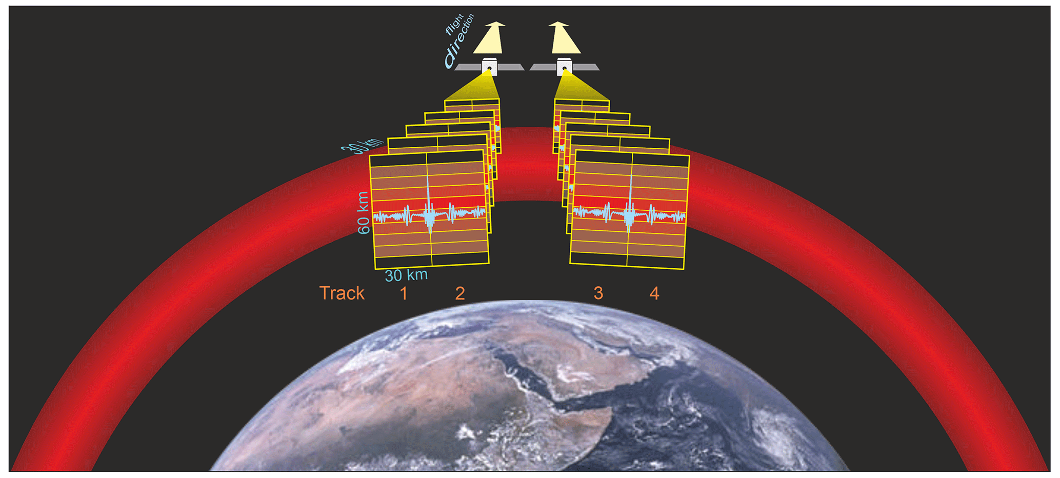
Figure 1Proposed observation geometry of two CubeSats flying in parallel and viewing backward. Each CubeSat carries an SHI which images the atmosphere in the vertical and generates a combined spectral–spatial view in the horizontal. By splitting the interferogram at zero optical path difference, both sides can be evaluated individually, allowing for four effective observation tracks.
Based on existing spaceborne limb-scanning observations that allowed distributions of the absolute GW momentum flux to be inferred (e.g., Ern et al., 2004; Alexander et al., 2008; Preusse et al., 2009a; Ern et al., 2011; Alexander, 2015; Ern et al., 2018), proposals were made on how a limb-imaging satellite mission could drastically improve our knowledge about GWs in the stratosphere (Preusse et al., 2009b, 2014). Such an instrument would provide 3-D data at good spatial resolution by high along-track sampling, tomographic retrieval in along-track slices (Ungermann et al., 2010a, b; Song et al., 2017), and across-track coverage by multiple tracks (illustrated in Fig. 1). Still, general restrictions due to the radiative transfer along the line of sight remain despite tomographic retrievals, and the observational filter allows observing only waves with horizontal wavelengths longer than 100 km (Preusse et al., 2009b). The first existing global observations exploited for 3-D data were nadir measurements of the Atmospheric InfraRed Sounder (AIRS) (Ern et al., 2017; Hindley et al., 2020). Although these data capture only long vertical wavelengths, i.e., high intrinsic phase speeds, they provide information on direction characteristics and allow demonstrating how backward ray tracing can be used for source identification from global data (Perrett et al., 2021). These examples are for the stratosphere only. Nevertheless, it is evident from such studies that a limb imager would provide novel information about GWs in the MLT.
The spatial sampling drives the complexity of the instrument and hence drives the cost of the mission. The spatial sampling requirements therefore need to be justified. The across-track dimension is provided by observing multiple tracks. An important question is therefore how many parallel tracks are required to gain reliable information about medium-scale GWs with horizontal wavelengths longer than 100 km (i.e., the ones visible to a limb sounder) and how these tracks should be spaced. On the one hand, it is obvious that the wider the overall swath is and the smaller the individual pixels are, the higher the likelihood is to acquire unprecedented scientific data. On the other hand, a larger number of tracks is a driver for increased instrument complexity and data downlink capacity. Besides the traditional satellite missions with a cost easily on the order of several tens of millions of Euro, an alternative option would be a CubeSat mission which takes fewer tracks of measurements but is still capable of providing a similar amount of information about GWs. Employing a spatial heterodyne spectrometer (SHS), the CubeSat instrument will provide good spectral resolution in the selected emission band, which is helpful to constrain the retrieval and obtain accurate temperature. Compared to an imager, however, the number of parallel tracks is lower. One of the aims of this paper is therefore to examine the minimum number of tracks required for deriving 3-D wave vectors of GWs from tomographic temperature observations.
From the above motivation, we deduce the following observation concept: airglow emissions at 762 nm from the oxygen atmospheric band (O2 A band) are particularly suited to gain information on MLT dynamics. Limb observations facilitate high vertical resolution during both day and night. Assuming rotational local thermodynamic equilibrium, the kinetic temperature around the tangent points can then be inferred from the relative line intensities. Using advances in CubeSat standard components, detector technology, and optics, a highly miniaturized spatial heterodyne interferometer (SHI) (Kaufmann et al., 2018) was developed for this purpose. This detection technology can be applied in a CubeSat constellation mission, which consists of two CubeSats, each hosting an SHI. By flying the two SHIs in parallel (illustrated in Fig. 1) and by splitting one interferogram into two left-hand and right-hand parts and separately mirroring each parts (see Sect. 3.5), thus splitting the horizontal field of view (FOV) in two, in total four independent observation tracks can be obtained from the proposed satellite observation geometry. High along-track resolution will be achieved using tomographic retrievals.
Based on limb-sounding four tracks simultaneously, we aim to observe medium-scale GWs of horizontal wavelengths longer than 100 km. In order to demonstrate the feasibility of quantifying GW properties by airglow limb observations, we will perform a full chain of end-to-end (E2E) simulations based on self-consistent model data. This validation of our methodology is based on GW parameters (e.g., GW momentum flux) that are derived from temperature residuals using the GW polarization relations (Fritts and Alexander, 2003; Ern et al., 2004; Preusse et al., 2009b). The feasibility will then be evaluated by inferring such GW parameters directly from the model data. This means that we choose the inferred GW parameters as a performance measure instead of a separate consideration of noise and resolution1. The stringency of validation by comparing distributions of GW momentum flux with reference distributions is discussed in Sect. 2.3. Phase speed spectra are essential for understanding the interaction with the background winds. However, all spectral investigations are dependent on the choice of the method and hence no absolute reference exists. We therefore compare in this paper how the spectra degrade when fewer tracks are employed.
In order to study the viability of a CubeSat mission, we will consider the following questions in this study.
-
Are polarization relations valid in the MLT region?
-
How few measurement tracks are required? Are four or even two tracks sufficient?
-
How much instrument noise can we afford in the temperature retrieval and wave analysis?
We address these three questions as follows: the assessment strategy is outlined in Sect. 2. Detailed introductions to models, tools, and the instrument are presented in Sect. 3. The outcomes of the assessment and answers to the questions are given in Sect. 4, followed by a discussion on scientific applications in Sect. 5. Finally, we summarize our findings (Sect. 6).
In this section we outline the strategy to address the questions formulated in the Introduction. We base our study on fields of winds and temperature from a free-running general circulation model (GCM) called the HIgh Altitude Mechanistic general Circulation Model (HIAMCM) (Sect. 3.1) resolving a larger part of the GW spectrum. Since the GCM simulates all dynamical features from first principles, wind and temperature structures of the model fields are consistent for all waves resolved. This consistency is essential for diagnosing deviations between the reference, analyzed GW momentum flux, and full end-to-end simulations: the smaller the deviations, the better the performance of the observation system. It should also be noted that while a realistic representation of the actual atmosphere by the model is important, potential deviations of the model fields from the simulated meteorological situation are not part of the assessment. To retain this consistency, winds and temperatures are separated into global-scale dynamics and GW fluctuations in the same way on the full model fields (Sect. 2.1). For an assessment we need a reference to evaluate the performance against. This is the zonal mean of zonal momentum flux derived from the model winds (Sect. 2.2). With this given, we can design the method (Sect. 2.3) to tackle the three questions posed in the Introduction.
2.1 Scale separation
The assessment is based on consistent GW-related fluctuations of temperature and wind velocities. This requires a scale separation between GWs on the one hand and global-scale dynamics on the other hand. This is usually performed by separating by zonal wavenumber.
For satellite data, traditionally waves up to zonal wavenumber 6 have been treated as global-scale waves and all remaining fluctuations as GWs (e.g., Fetzer and Gille, 1994; Preusse et al., 2002; Ern et al., 2018). This separation is used as wavenumber 6 is the highest wavenumber which can be reliably resolved by a single-observation-track low Earth orbit (LEO) satellite (Salby, 1982). Such a detrending method via space–time spectral analysis has been used for, e.g., SABER data (Ern et al., 2018).
For model studies a much higher separation wavenumber has often been used. Strube et al. (2020) have shown that separation wavenumbers 6 to 8 are sufficient for the stratosphere and that removing wavenumbers up to 40 significantly cuts into the GW part of the spectrum. For studies including the UTLS Strube et al. (2020) recommend zonal wavenumber up to 18 for scale separation. In this study we also use zonal wavenumber 18 with an additional meridional Savitzky–Golay filter of third-order polynomials over 5∘ of latitude. This defines our large-scale background, which is subtracted from individual temperature values in order to define residuals.
A satellite in a sun-synchronous orbit acquires data at a continuously evolving observation time but fixed local time for a given latitude on ascending and descending orbit legs. Such a sampling cannot be generated from model data which are sampled at fixed UTC and sampling intervals of O(1 h). Switching between model fields as the orbit evolves would result in jumps at the switching points, while interpolation in time would smooth the interpolated GW fields in an unpredictable manner. In this study we therefore use a single model snapshot (1 January 2016 at 06:00 UT). Synthetic orbit data generated in this manner allow addressing all questions stated in the Introduction. In particular, a fixed UTC has the advantage that the synthetic orbit data can also be compared to the reference of zonal mean GWMF from full model fields, which is the basis of our assessment.
2.2 Zonal mean momentum flux: a true reference
At the end, we aim to quantify the vertical flux of horizontal pseudomomentum of GWs (Fritts and Alexander, 2003):
where Fpx indicates its zonal component and Fpy is its meridional component. ρ is the background density, f the Coriolis parameter, the intrinsic frequency, and u′, v′, and w′ the wind vector perturbations due to the GW in zonal, meridional, and vertical directions, respectively; eastward, northward, and upward are positive signed. The overline denotes the average over a full or multiple wavelengths of the wave. The vertical gradient of the pseudomomentum flux (PGWMF) determines the acceleration of the background wind on a rotating sphere. However, determining from a given 3-D data set involves some kind of wave analysis and, accordingly, assumptions. On the other hand, the zonal mean of zonal momentum flux () is a true reference as it depends on the wind fluctuations only and as on the cyclical domain of longitude all waves are properly averaged.2 If not explicitly stated otherwise, we will hence consider GW momentum flux (GWMF) without the correction for Coriolis force in our assessment.
2.3 Method of assessment
The E2E approach for evaluating the performance of the proposed mission concept is illustrated in Fig. 2. We employ HIAMCM data (Becker and Vadas, 2020, see Sect. 3.1) for a realistic, self-consistent basis of the E2E simulations. The distributions of temperature, density, and wind velocities are separated for large-scale structures such as planetary waves and tides on the one hand and small-scale residuals due to GWs on the other hand. We consider both wind and temperature data. Temperatures are the observation target of the measurement method. From the winds we gain our reference for the assessment. As described in the Introduction, zonal mean GWMF calculated directly from the wind perturbations provides an unambiguous reference of truth against which we can compare the values from simulated observations and thus quantify the influence of the various assumptions or constraints needed for observing GWMF with a real instrument.

Figure 2Schematic flow diagram of the assessment steps to address the three major questions highlighted in yellow diamond boxes. The assessment is based on comparison with zonal mean GWMF calculated directly from the model winds and considered here as the reference of truth. From the top down further assumptions and/or constraints are added as the tested data become more similar to the real observations.
The first question which we address is the applicability of the polarization relation for the MLT. GWMF can be deduced from 3-D temperature data by determining the 3-D wave vector assuming polarization and dispersion relations (see Sect. 4.1). In order to test the validity of this approach, we apply our wave analysis – the small-volume 3-D sinusoidal fit method (S3D; Sect. 3.7), which provides wave amplitudes and 3-D wave vectors based on small sub-volumes of the data set considered – directly to the full model data and compare thus generated zonal mean GWMF with our reference.
The second question regards the number of tracks required for reliable GWMF quantification (see Sect. 4.2). For this assessment, we sample model residual temperatures onto various synthetic measurement geometries for different numbers of observation tracks, apply S3D and, again compare against the reference.
Third, we assess the influence of the observation technique which comprises both the observational filter as a general limitation of limb sounding and the specific instrument parameters (see Sect. 4.3). This assessment therefore encompasses all steps of observation starting from synthetic radiances generated by forward modeling, a simplified instrument model adding realistic noise, and a tomographic retrieval. Again, S3D is applied to the outcome of the full E2E simulations, and zonal mean GWMF is assessed against the reference. Different noise levels are tested in order to determine the robustness against instrument performance.
This section describes the atmospheric circulation model and the radiative transfer model we base our study on, introduces the SHS instrument proposed for the observation, and gives an introduction to the wave analysis and retrieval tools employed.
3.1 HIAMCM
The HIAMCM (HIgh Altitude Mechanistic general Circulation Model) (Becker and Vadas, 2020; Becker et al., 2022) is a new high-altitude version of the KMCM (Kühlungsborn Mechanistic general Circulation Model). The HIAMCM employs a spectral dynamical core with a terrain-following hybrid vertical coordinate. This includes a correction for non-hydrostatic dynamics and physically consistent thermodynamics in the thermosphere. The current model version uses a triangular spectral truncation at a total wavenumber of 256, which corresponds to a horizontal grid spacing of ∼ 52 km. The altitude-dependent vertical resolution includes 280 full levels. The level spacing is dz ∼ 600 m below z ∼ 130 km, with dz increasing with altitude farther above and dz ∼ 5 km above z ∼ 300 km.
The HIAMCM captures atmospheric dynamics from the surface to approximately 450 km. GWs are simulated explicitly with an effective resolution that corresponds to a horizontal wavelength of ∼ 200 km. Non-resolved scales are parameterized by macro-turbulent vertical and horizontal diffusion based on the Smagorinsky model. Since molecular viscosity is taken into account for both vertical and horizontal diffusion, the HIAMCM does not require an artificial sponge layer. Resolved GWs are dissipated self-consistently by molecular diffusion in the thermosphere above ∼ 200 km and predominantly by macro-turbulent diffusion at lower altitudes. These features allow the HIAMCM to capture the generation, propagation, and dissipation of medium-scale GWs, including their interactions with the large-scale flow and the generation of secondary and tertiary waves. This capability is essential to simulate GW dynamics in the MLT (Becker and Vadas, 2018) and at higher altitudes (Vadas and Becker, 2019).
The HIAMCM employs radiation and moist convection schemes that are simplified compared to comprehensive methods. Though convection is only present in the troposphere, it is essential as a source of upward-propagating waves, namely GWs, tides, and tropical wave modes, and is thus also highly relevant for the dynamics in the MLT. Furthermore, the model does not include a chemistry module, and ion drag is the only ionospheric process that is accounted for. To distinguish these idealizations from methods employed in community models, the HIAMCM is said to be a mechanistic model. Nevertheless, the key features of a climate model (topography, simple ocean model, radiative transfer, boundary layer processes, tropospheric moisture cycle) are fully taken into account. Also note that the HIAMCM is currently the only GW-resolving whole-atmosphere model that can be nudged to reanalysis in the troposphere and stratosphere, allowing for the simulation of observed events (Becker et al., 2022).
3.2 Orbit simulator
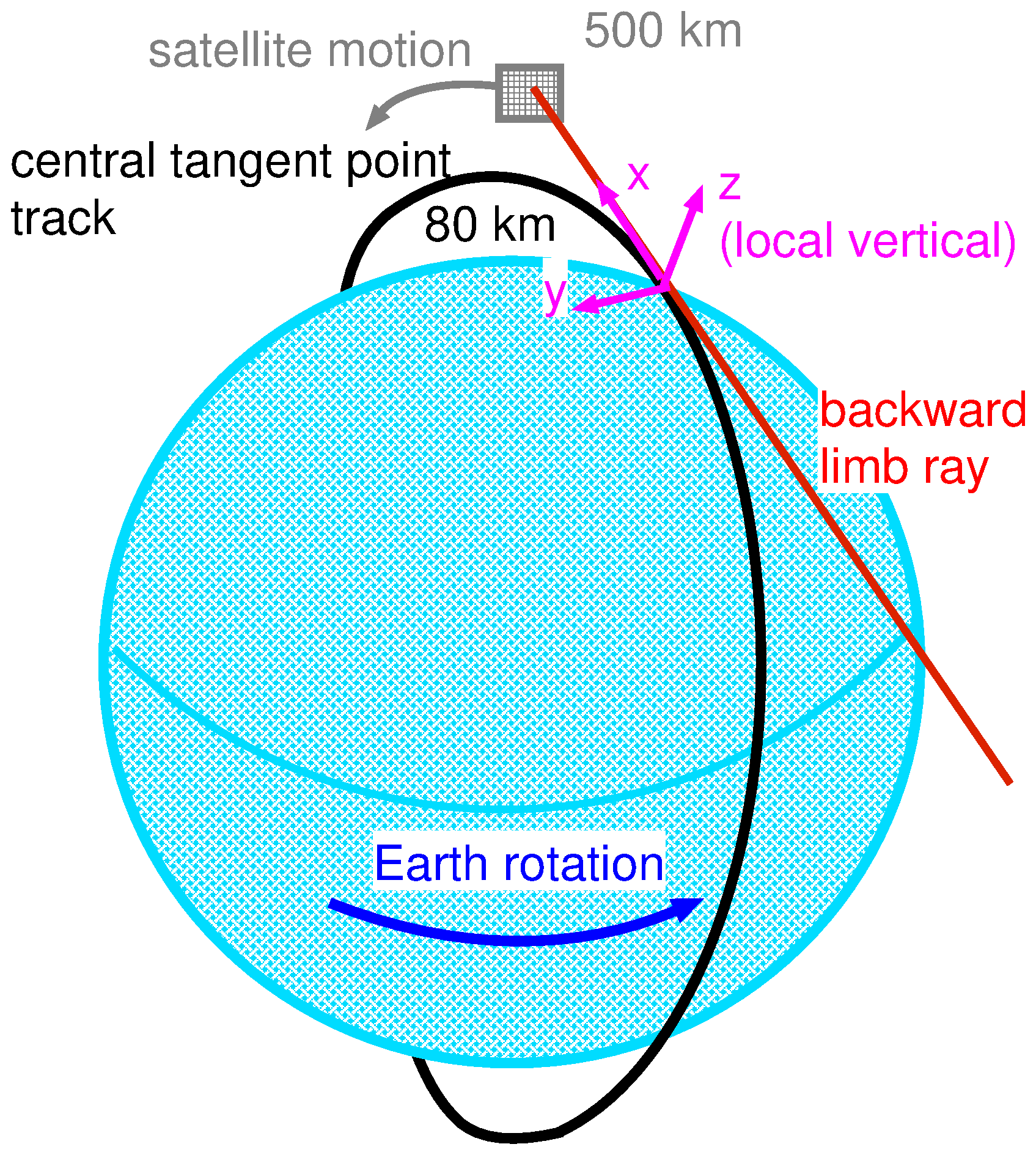
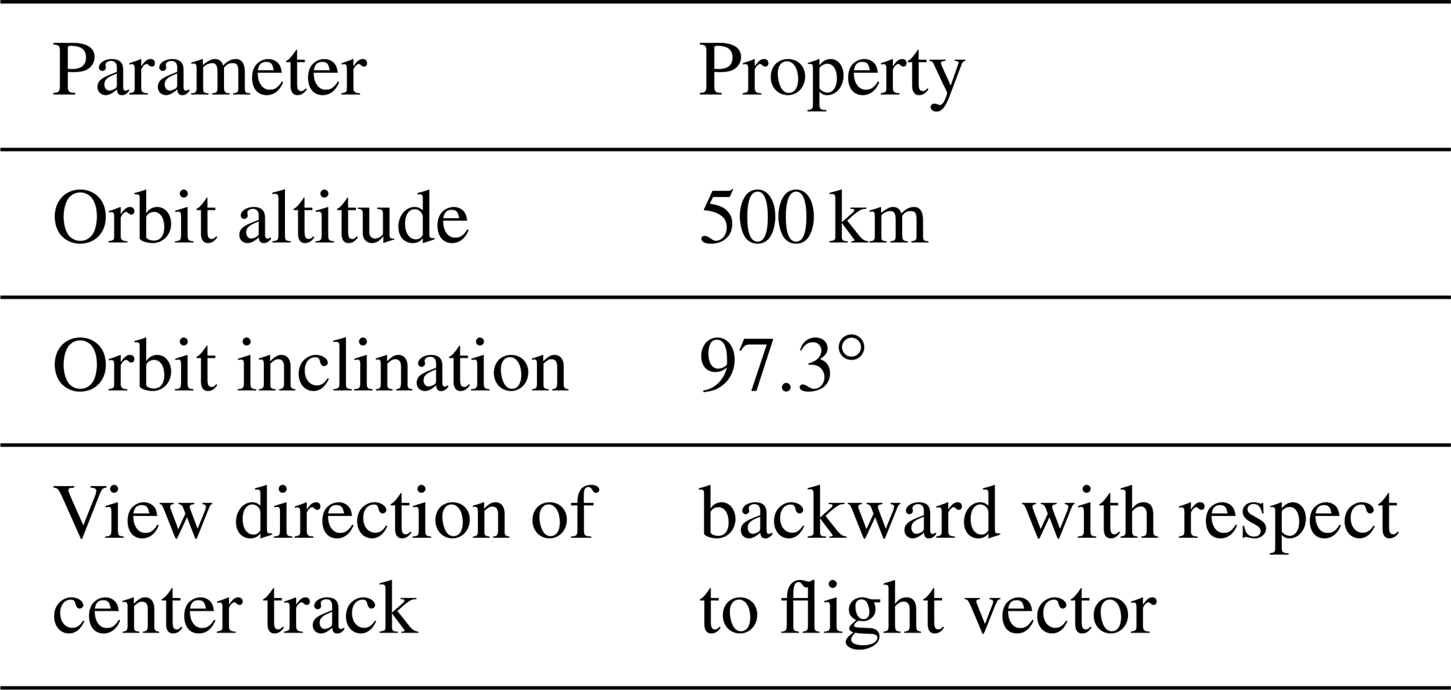
The simulation of the orbit (illustrated in Fig. 3) is based on a fixed orbit inclination, orbit altitude (shown in Table 1), and start longitude at the beginning of the day. Assuming a spherical Earth and constant gravity acceleration scaled to orbit altitude the in-orbit velocity is determined. A time series of orbit positions on Earth surface is calculated from the satellite position on the orbit fixed in space and the rotation of the Earth. A grid for atmosphere representation (atm-grid in the following) is then generated based on the tangent points of the backward-viewing direction for 80 km altitude and spanning a local rectilinear grid with the x direction along this tangent point track, a y direction perpendicular to this tangent point track, and the local vertical. Both satellite position and atm-grid are then used to build a complete set of matching tangent points for radiative transfer and retrieval simulations as described in Sect. 3.3 and 3.6. The basis for the radiative transfer simulations is the atmospheric quantities such as temperature and pressure interpolated from the longitude–latitude grid of the general circulation model to the atm-grid by means of spline interpolation.
3.3 O2 A-band airglow photochemistry and radiative transfer process
This section describes the photochemical processes which initiate the generation of the O2 A-band emission, followed by a short description of radiative transfer process propagating the radiance to the instrument.
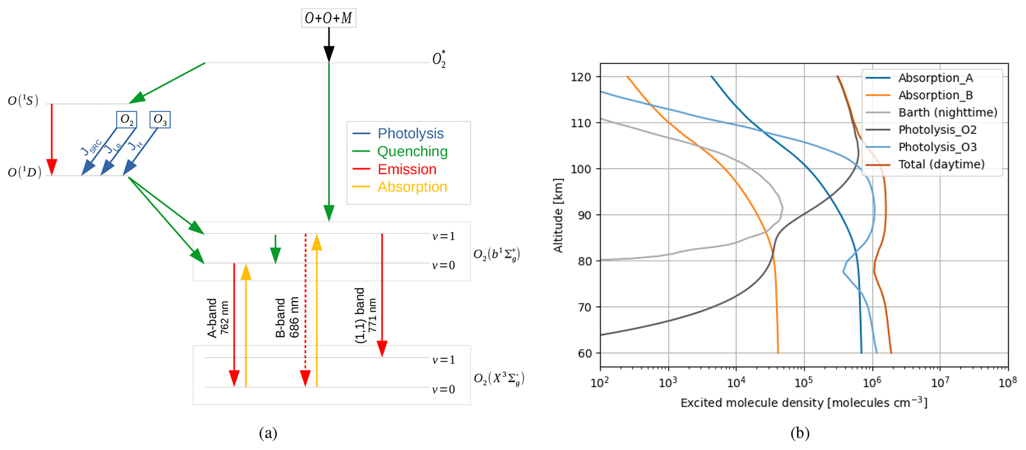
Figure 4(a) Schematic of the production of excited-state ; dashed lines indicate neglected transitions. (b) Number density of excited O2 molecules due to the different production mechanisms using HAMMONIA model data (Schmidt et al., 2006); note that during daytime all five production mechanisms are active, whereas during nighttime only the Barth process is active.
O2 can be present as 16O2, 17O16O, or 18O16O; the latter two can be neglected due to their low abundance, as shown by Slanger et al. (1997). In general, an excited molecule can be in one of multiple electronic states; for each electronic state the radicals can be in one of multiple vibrational states. The transitions between different electronic–vibrational states form atmospheric emission and absorption bands. Each band consists of multiple emission lines due to the transitions within multiple rotational states of vibrational states. We measure the A-band emission at 762 nm, which is the electronic transition from the second excited state to the ground state . A detailed description of the dayglow O2 A band is given by Sheese (2009), Bucholtz et al. (1986), and Zarboo et al. (2018). It has three sources, which are depicted in Fig. 4a.
First, the excited state can be produced by photon absorption in the atmospheric bands. Bucholtz et al. (1986) show that the γ-band absorption from to can be neglected, and hence it is not shown in Fig. 4a. Only the absorption in the A and B bands is therefore considered. The excited molecules in are rapidly deactivated to via a quenching process. Slanger et al. (1997) argue that the B-band emission at 686 nm is insignificant compared to the quenching process and can be neglected. The emission in the (1,1) band is considered. The second source is due to photolysis of O2 in the Schumann–Runge continuum (JSRC) and at Lyman α () and due to the photolysis of O3 in the Hartley band (JH). It produces excited atomic oxygen O(1D), which transforms to due to collisional excitation with O2 in ground state. The third source is a chemical source, which is independent of solar radiation and hence also present during nighttime. The source of this process is a three-body recombination of atomic oxygen, producing electronically exited radicals. From there, is produced through a direct quenching process or a chain of quenching processes, going through O(1S) and O(1D). This process was first described by Barth and Hildebrandt (1961) and is called the Barth process. Since some of the related rate coefficients are not well known, McDade et al. (1986) proposed a model with fitting parameter to describe the Barth process. A detailed description of the calculation of O2 A-band emission is given in Appendix A. Figure 4b shows the number density of excited O2 molecules due to the different production mechanisms using HAMMONIA model data (Schmidt et al., 2006). Note that during daytime all five production mechanisms are active, whereas during nighttime only the Barth process is active.
The O2 A-band airglow emissions are transmitted through the atmosphere before they are detected by an instrument. The observed airglow spectra are integrated slant-path radiances along the instrument viewing line of sight (LOS). For limb observations, the emissions from the lowermost tangent points along the LOS contribute the most to the integrated radiances provided that the atmosphere is still optically thin for the emission lines.
Due to the high abundance of the ground-state O2 molecule in the atmosphere and its self-absorption effect, the emitted O2 A-band radiance can only partly pass through the atmosphere and reach the instrument detector. This radiative transfer process is described by the Lambert–Beer law, and the observed spectral irradiance intensity can be written in integral form as
where ν refers to the wavenumber of the spectral line, s denotes the LOS distance, D(ν) represents the line shape broadening profile, which is dominated by Doppler broadening in the middle and upper atmosphere, n(s) is the number density of O2, and σ is the O2 absorption cross-section.
In the lower atmosphere, nearly all O2 A-band emissions are self-absorbed. Thus, O2 A-band airglow cannot be detected on the ground. During daytime, the O2 A-band emissions are sufficiently strong for observations at altitudes from 60 to 120 km and are reduced to the range of 80 to 100 km during nighttime. In the simulation, we have assumed optically thick conditions for the center wavelength of the emission lines (see Appendix B).
3.4 Spatial heterodyne interferometer
A spatial heterodyne interferometer is based on the principle of a Michelson interferometer, but the two mirrors are replaced by fixed tilted gratings. The simplified concept of the SHS is shown in Fig. 5. Light of a frequency within the spectral bandpass enters the instrument along the optical axis. Light of each frequency is split into two waves by the beam splitter and diffracted and reflected by the gratings. The two waves arrive back to the beam splitter, producing an interference pattern, which is forwarded to the detector. Considering multiple emissions within the bandpass, an interferogram consists of multiple superposed interference patterns along the x axis, which can be described by sinusoidal waves. The spatial frequency of the produced fringe pattern follows from the grating equation, denoted by
where σ is the wavenumber of the incoming light, θL the blaze angle of the gratings, also called the Littrow angle, d−1 is the grating groove density, m is the diffraction order, and γ the outgoing diffraction angle with respect to the Littrow angle. The Littrow wavenumber is the wavenumber where γ=0, thus
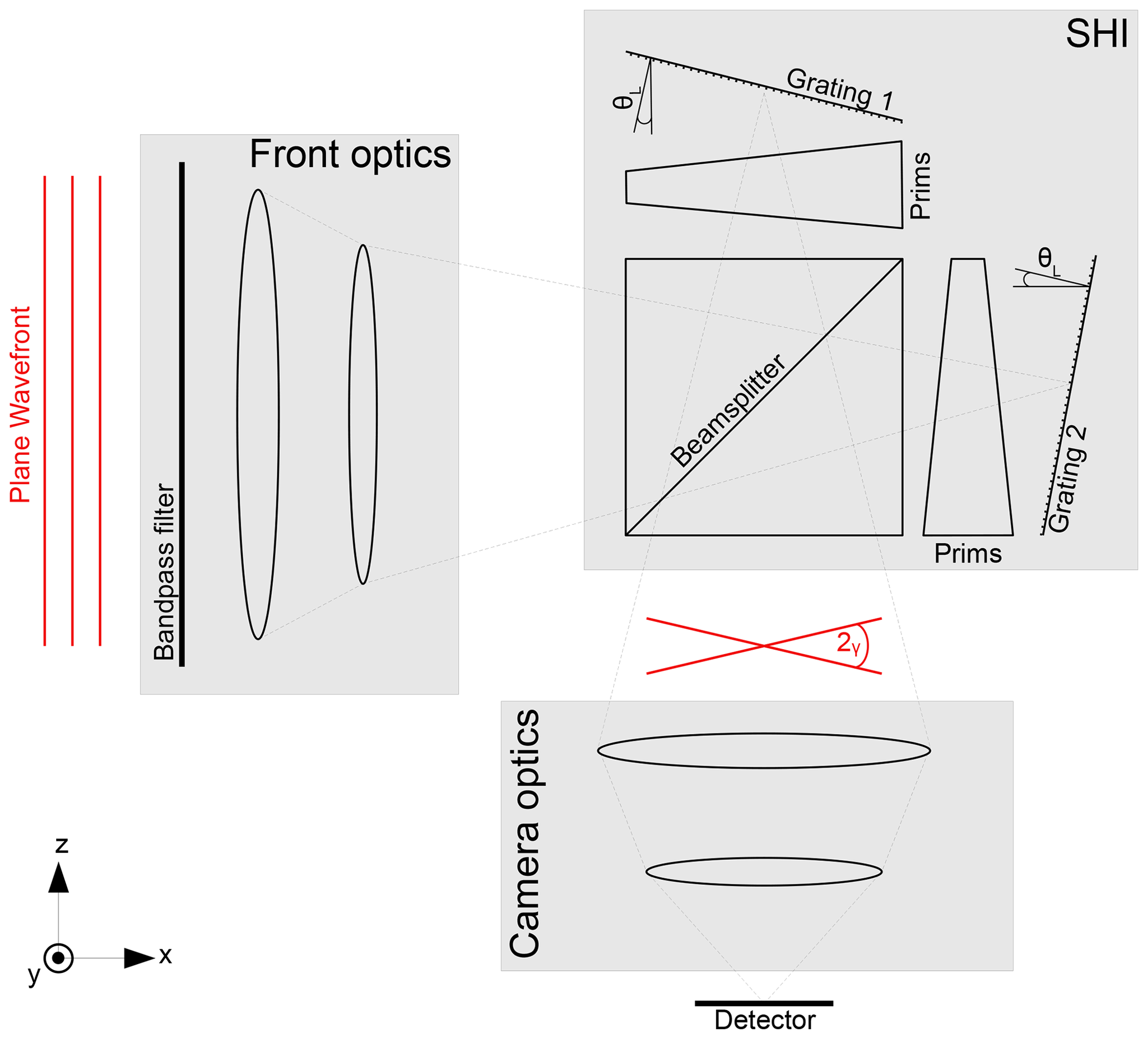
Using Taylor expansion, Harlander et al. (1992) show that the spatial frequency is dependent on the wavenumber by
where M is the magnification factor introduced by the camera optics.
This equation shows that the relation between spatial frequency and wavenumber is symmetric around the Littrow wavenumber.
Following Roesler and Harlander (1990) and Deiml (2017), an ideal one-dimensional interferogram along the x axis can be described by
where B is the spectral radiance, and b0 and b1 are the lower and upper bound of the spectral filter, respectively.
The interferogram is transformed into a spectrum by Fourier transformation. Figure 6 shows the O2 A-band emission for two temperatures and the corresponding spectra as seen by the instrument. The temperature dependency as seen in the lower panel of Fig. 6 is used to retrieve temperature.

Figure 6Modeled O2 A band seen by the SHI instrument for temperature at 200 and 210 K. The spectra are presented by the Dirac impulses such that the sum over all emission lines is equal to 1; below the relative intensity difference between the spectrum at 200 and 210 K is shown. The dashed line shows the theoretical filter curve and the dotted vertical line the designed Littrow wavenumber of the AtmoLITE instrument. The gray shaded area shows the spectrum convolved by the instrument line shape; r = 1.43 cm−1 is the spectral step size.
A silicon-based detector is used in this instrument. The operation in ambient to cool conditions gives a shot-noise-limited system for integration times of 1–10 s (Liu et al., 2019). Shot noise can be modeled by a Poisson process with mean and variance equal to the signal. For a signal above 10 counts, the Poisson distribution approximates a normal distribution about its mean. Thus, for simplicity the shot noise is approximated by additive white Gaussian noise with standard deviation equal to the square root of the signal in each pixel.
3.5 Split of the interferogram
Revisiting Fig. 5, the front optics map the captured atmospheric scene onto the gratings. In a similar fashion, the camera optics map the image on the grating to the image on the detector. Accordingly, the SHI performs a spatial mapping of the atmospheric scene onto the detector. As described in Sect. 3.4, the spectral information is contained on the x axis due to constructive and destructive interference induced by the gratings. The interferogram therefore contains spatial information on the vertical (y axis) and superimposed spectral and spatial information on the horizontal axis (x axis). This is utilized when splitting the interferogram at zero optical path difference (ZOPD) and using each half individually. The spectral information is fully contained in one half as the interferogram is symmetric around the ZOPD by definition. Mirroring each side around the ZOPD gives a full interferogram for each side, which can be employed to derive two independent temperatures along the horizontal axis. Each interferogram then contains temperature information of the associated side of the field of view. The concept to mirror the interferogram at the ZOPD has already been used by Johnson et al. (1996) for the far-infrared spectrometer (FIRS)-2 and by Gisi et al. (2012) for the TCCON FTIR spectrometer to gain a higher resolution. However, Ben-David and Ifarraguerri (2002) and Brault (1987) point out that the phase correction including finding the correct ZOPD is crucial.

Figure 7Simulation of interferogram split assuming a linear temperature gradient. Panel (a) shows the temperature gradient from 200 to 220 K across the horizontal field (solid line) with each side symmetrically extended around the center (dashed lines); the red circle and the blue diamond indicate the location of the retrieved temperature for the left and right hand side. Panel (b) shows the left symmetrically extended interferogram. Panel (c) shows the temperature retrieval of (b). Panel (d) shows the difference between the left and right symmetrically extended interferogram. Panel (e) shows the difference between the left and right symmetrically extended raw spectrum.
The following simulation demonstrates that averaged temperatures of the respective parts of the field of view can be recovered from an analytical interferogram, theoretically allowing two independent cross-track measurements with one instrument. We assume a linear temperature gradient across the horizontal field. We simulate each pixel with the associated temperature and assemble the full interferogram pixel by pixel. Subsequently, the interferogram is split at the ZOPD, and each side is symmetrically extended to get two full interferograms. Each side can be then used to retrieve a temperature. Figure 7 shows the simulation result of an ideal interferogram without noise using a simple temperature retrieval which minimizes the squares of the residuals. The red circle and the blue diamond in Fig. 7a indicate the retrieved temperature. Mapping the retrieved temperatures back onto the initial temperature gradient results in two data points which are about 17 km apart. Note that the two retrieved temperatures are shifted towards the center and are not located at the spatial centers of each side at ±15 km. The Fourier transformation is a weighted sum over the samples in the interferogram. Areas which deviate the most from the mean of the interferogram therefore contribute the most to the shape of the spectrum. Since the area around the ZOPD deviates the most from the interferogram's mean, the temperature information of that area contributes the most to the retrieved temperature. This causes the shift towards the center. An in-depth validation using calibration and orbit data considering noise and instrument errors is the content of future research.
3.6 Tomographic retrieval for generating 3-D atmospheric volumes
Retrieving temperatures from measured limb spectra is a classic inverse problem. That is, we have a radiative transfer model that can compute measured spectra from an assumed atmospheric state (forward model), but the inverse problem is much harder, since it is typically both underdetermined (multiple atmospheric states could result in the same set of measurements) and ill-posed (there might be, in theory, no atmospheric states that could result in a given real-life measurement affected by instrument noise and other error sources). Such a problem is solved using the forward model and a mathematical framework for inverse modeling (e.g., Rodgers, 2000). The main idea of this approach is iterative minimization of the following function (called cost function):
Here y is a set of measurements taken by the instrument, and x is the candidate atmospheric state. F(x) is the forward model; it maps an atmospheric state x to the set of measurements that the instrument would acquire if the atmosphere was indeed in the state x. xapr represents our prior knowledge of the atmospheric state. In our case that is an estimate of the large-scale temperature structure of the atmosphere without gravity waves. and are positive-definite symmetric matrices (covariance matrices).
The first term on the right-hand side of Eq (7) quantifies how closely the atmospheric state x matches the observations y. One can construct the covariance matrix knowing the measurement error characteristics typical for the instrument in question. The second term quantifies how likely the atmospheric state x is given our prior knowledge about the atmosphere. This knowledge includes both the base state of the atmosphere xapr and more general considerations (such as the fact that large spatial discontinuities in temperature are unlikely) that are taken into account when constructing (Ungermann et al., 2010a). Equation (7) is solved iteratively using the Levenberg–Marquardt algorithm (Marquardt, 1963) and a conjugate gradients solver. For both the forward model and the inverse modeling we need a computationally efficient implementation.
Here, we employ the JURASSIC2 forward model (e.g., Ungermann, 2013) to simulate the spectra based on a 2-D discretization of the atmosphere along the satellite track. This model was enhanced for this study by a simple adjoint line-by-line model dedicated to the simulation of the O2 A band (see Sect. 3.3). The inversion uses the JUTIL Python library to bring the synthetic and measured spectra in agreement using a truncated conjugate gradient trust region method (e.g., Ungermann et al., 2015).
In order to perform a full end-to-end test, noise is added to simulated observations to emulate instrument performance. To generate the noise in the synthetic measured spectra, we compute from the spectrum the number of photons hitting (on average) one detector pixel per second and use this number to determine Gaussian noise assuming that the instrument is shot-noise-limited and the dark current is negligible; i.e., the 1σ is computed from the square root of number of photons. Note that we assume an efficiency of 0.2; i.e., only one-fifth of inbound photons will end up in the modulated part of the interferogram. This noise is then reduced according to assumed averaging in time and space (4.5 s integration time, 13 vertical detector rows, four horizontal detector columns).
The individual measurement tracks of the proposed satellites are treated separately from one another, and each constitutes a separate 2-D slice at the orbital plane of the satellite or very close to it (Fig. 8). Limb measurement geometry and backward-viewing direction result in each air parcel within the 2-D slice being observed from multiple points of the satellite orbit. This allows reconstructing the 2-D temperature cross-section in a tomographic fashion. The full 3-D state is reassembled afterwards from the individually retrieved 2-D slices. The satellite speed allows gathering all relevant measurements for a spatial sample in the order of minutes, which is short compared to typical periods of gravity waves observable by our instrument.
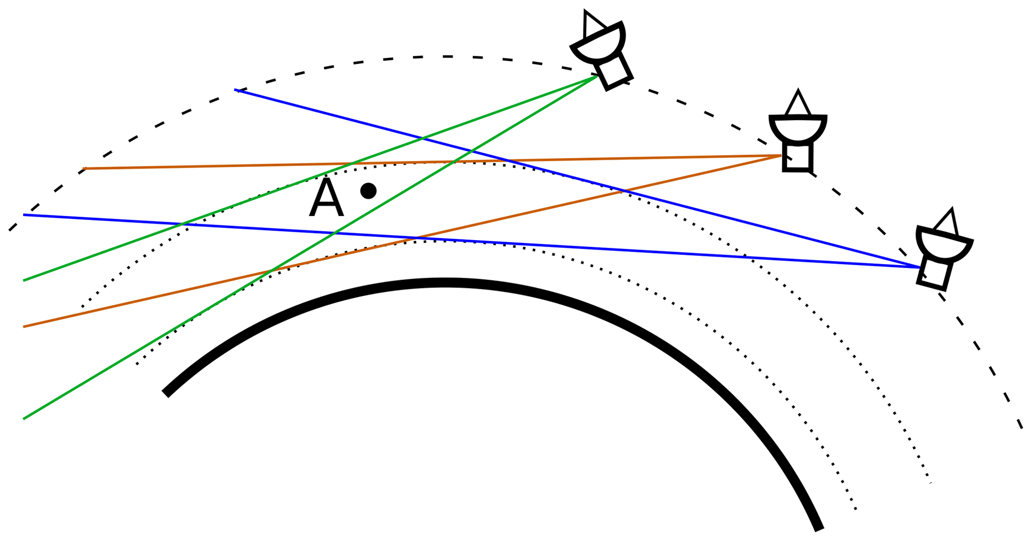
Figure 8The principle of 2-D tomography. The field of view of the satellite within the orbital plane is shown for different satellite positions along the orbit. A point A inside the airglow layer lies within the field of view for all three positions, and therefore airglow radiance at point A contributes to observed radiances at all these positions and every position in between. We can use the observations to solve for airglow radiance at point A (and all other such points) using inverse modeling.
As explained in Sect. 3.3 there are more excitation mechanisms and higher emissions during daytime than during nighttime. For one retrieval, we therefore split the orbit at the position of the terminator in roughly two equal halves, one containing the daytime and the other containing the nighttime measurements (even though we currently apply the same retrieval settings to both). We then lengthen the two orbit parts by an additional ≈ 1500 km on both ends. Horizontally, a sampling of 30 km is used, while the vertical range is sampled in 1 km steps from 60 to 120 km and in 2 km steps above (Table 2).
Table 2Summary of detector and sampling properties.
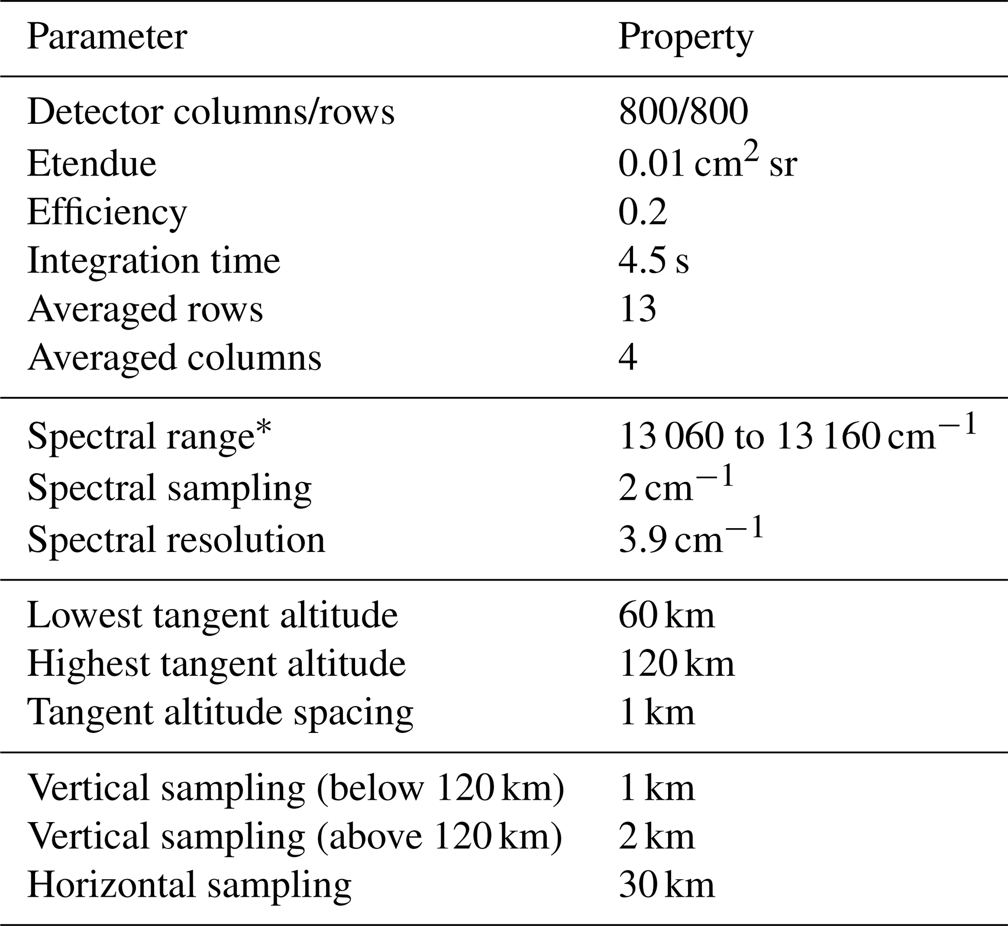
∗ The spectral wavenumber is defined here as λ−1, where λ is the wavelength of emissions or absorptions.
The forward simulations employ a regular grid of two rays per detector row, which are combined assuming a line spread function of Gaussian shape with 1σ corresponding to the height of the row.
The spectra range from 13 060 to 13 160 cm−1 with a sampling distance of 2 cm−1 and a spectral resolution (full width at half-maximum, FWHM) of ≈ 3.9 cm−1 due to the employed strong Norton–Beer apodization (Norton and Beer, 1976). More details about the simplifying assumptions for the forward model in the tomographic retrieval are given in Appendix B.
3.7 JUWAVE S3D wave analysis
In this study we investigate GWs in a narrow stripe (small swath width) of observations along the tangent point tracks. This requires an analysis method which can, at least in one direction, analyze waves with notably longer wavelengths than the size of the analysis volume. In addition, the vertical wavelength of gravity waves is refracted by the background wind; this contradicts the assumption of a stationary wave spectrum over the range of the analysis volume, which is made, e.g., by Fourier transform. For such applications, the small-volume sinusoidal fit method (S3D) was developed and tested for the purpose of GW analysis in small observation volumes and for highly localized GW fields (Lehmann et al., 2012).
In this method, the observation volume or model domain is divided into small sub-volumes and a sinusoidal fit is performed on each sub-volume:
where is the temperature fluctuation at the location xi, and kjxi is the scalar product between the wave vector of the j wave component with the spatial coordinate vector of the i point in the analysis volume. The wave components j are determined sequentially by subtracting the wave field of component j from the fit volume before fitting j+1. In this study, three wave components are fitted. Amplitudes and wave vectors are determined via least squares fit: amplitudes are determined analytically and wave vectors via a variational approach. The minimum χ2 from a steepest descent method and a nested interval method is selected.
The size of the analysis cube is selected in a way that most of the spectral content has a wavelength of , with λd being either the horizontal or the vertical wavelength and csd the analysis volume diameter. This choice is motivated by previous sensitivity studies (Preusse et al., 2012) and will be discussed further in Sect. 4.2.1. In particular, we find that a vertical cube size of 15 km comprises the spectral power in the MLT region almost entirely. In the lower thermosphere, which is analyzed for consistency reasons as well, larger cube sizes are needed. To retain only reliable fits, we omit all fits with derived horizontal or vertical wavelengths larger than 3 times the respective cube size from evaluation. In order to enhance the vertical resolution and hence to better capture the loss of GWMF by the approach to a critical level at the MLT wind reversal, a refit of only amplitude and phase based on the wave vector from the initial fit is performed. For this study, we keep the horizontal cube size the same but reduce the vertical cube size to 5 km, with the exception of Sect. 4.1, where the results are obtained through a vertical cube size reduction to 4 km. In the same section, the initial cube grid consists of cubes with sizes 300 km × 300 km × 15 km (at 75 km altitude) and 600 km × 600 km × 20 km (at 130 km altitude).
The synthetic observation data have a fixed sampling in the x, y, and z direction, on which the analysis cube size is defined via the number of sampling points. For the model data, a fixed model sampling in terms of degrees longitude in the zonal direction means a coarser (in distance) sampling close to the Equator and a finer sampling at high latitudes due to the shorter distance between two respective longitudes at higher latitudes. Therefore, the size of a fixed cube is specified in kilometers instead of degrees and the number of fitting points is adapted accordingly. This ensures that the same part of the spectrum is targeted independent of latitude along the longitude direction.
The results of S3D are expected to be a good compromise between spatial and spectral representation. It has been shown by Lehmann et al. (2012) that the spectral distribution composed of all S3D wave fits in a given region reproduces the spectral content obtained via Fourier analysis of the same region well. At the same time, waves are localized well and can be attributed to individual source features.
In this section we use the methods described in Sect. 3 and follow the assessment approach outlined in Sect. 2 in order to quantify to which accuracy GWMF can be inferred from MLT limb observations and how many independent across-track points (i.e., how many measurement tracks) are required. The assessment measure is the comparison of global GW momentum flux values from simulated temperature observations to the values directly obtained from wind fluctuations of the full model fields. In addition, we consider how well spectral information is conserved when reducing the number of observation tracks. The assessment starts from consistent fluctuations in temperature and wind velocities after scale separation applied to a single snapshot of full model data (see Sect. 2.1 and Fig. 2); i.e., the scale separation is applied but not subject to the assessment.
4.1 Polarization relations
In the proposed mission concept GWMF is inferred from 3-D temperature structures. This requires that (a) polarization relations are also valid in the MLT under nonlinear conditions of many GWs approaching a critical level and that (b) a few-wave decomposition approach such as S3D is an adequate method for determining the 3-D wave vectors of the leading GWs (see Question 1 in Fig. 2). This is tested here using the approach from Sect. 2.3 (see the data flow to the upper yellow diamond of Question 1 in Fig. 2).
In order to verify that the momentum flux based on the S3D-derived wave parameters can be correctly calculated, a comparison with momentum flux estimates directly from wind residuals is carried out. As outlined in Sect. 2.2, we use zonal mean GWMF (without the correction for Coriolis force) as a true reference:
where Fx and Fy are the zonal and meridional components, respectively. Following the derivation of the vertical flux of horizontal gravity wave pseudomomentum by Ern et al. (2004), we express Eq. (9) in terms of the residual temperature wave amplitude , wavenumbers k, l, and m, and intrinsic frequency as
In Eq. (10), N is the buoyancy frequency, T is the background temperature, and the factor converts from pseudomomentum to momentum. Equation (10) is a simplified expression omitting two correction terms which are discussed in the supporting material to Ern et al. (2017) and relevant only to high-frequency GWs not considered in this study. The wave parameters of Eq. (10) are acquired through S3D analysis of temperature residuals of the HIAMCM data.
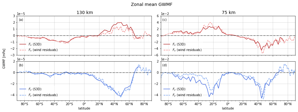
Figure 9The zonal mean vertical flux of zonal (red) and meridional (blue) momentum. Dashed lines show GWMF calculated from wind residuals (Eq. 9), while solid lines are calculated using wave vectors and residual temperature amplitudes (Eq. 10). Panels (a) and (b) show the fluxes at 130 km altitude, while panels (c) and (d) show fluxes at 75 km. Wind-based fluxes have been smoothed by averaging over 4 km altitude bins centered at the specified altitude and by averaging over 5∘ latitude bins.
Figure 9a and b show the zonal and meridional components of GWMF at an altitude of 130 km. The temperature-derived flux, based on wave parameters from global evenly distributed S3D analysis volumes, is in good agreement with the wind-based method used for reference. There is dissimilarity in the zonal GWMF at around 50∘ N, indicating a region of strong wind shear and/or a breakdown of the validity of the linear approximation. Likewise, at lower altitude the methods are consistent, with some differences in the zonal component around 25∘ S (Fig. 9c) and in the meridional component across the Southern Hemisphere midlatitudes (Fig. 9d), suggesting dynamics that are not completely captured. As a whole, the results from the two different methods are in good agreement and confirm that Eq. (10), based on wave properties from S3D analysis, is suitable for studying wave dynamics in the MLT.
4.2 How few tracks are required?
One of the major questions concerning our approach is how many measurement tracks are necessary to sufficiently derive the GW parameters in the MLT region within the framework of the proposed two-CubeSat observation strategy (see Question 2 in Fig. 2). For this purpose we test the E2E simulations with a series of a varying number of tracks and swath widths. The detailed results are presented in this section with a focus on the interpretation and intercomparison of GW vectors and zonal mean momentum flux values. All results presented in this subsection are either from sampled orbit data or full E2E simulations (see Sect. 2.3 and the data flow to the middle yellow diamond of Question 2 in Fig. 2).
4.2.1 Analysis of wavelength spectra
Spectra of PGWMF as a function of horizontal and vertical wavelengths are considered for two reasons. First, the choice of the cube size restricts the long wavelength limit of the analyzed spectrum. As described in Sect. 3.7, the desired wavelengths should ideally be in a range of [, 3] times the cube size, and wavelengths larger than 3 times the cube size are rejected. We hence need to verify that our cube size choice does not cut off major parts of the spectrum. Second, the wavelength spectrum should remain (largely) unchanged when reducing the number of tracks.
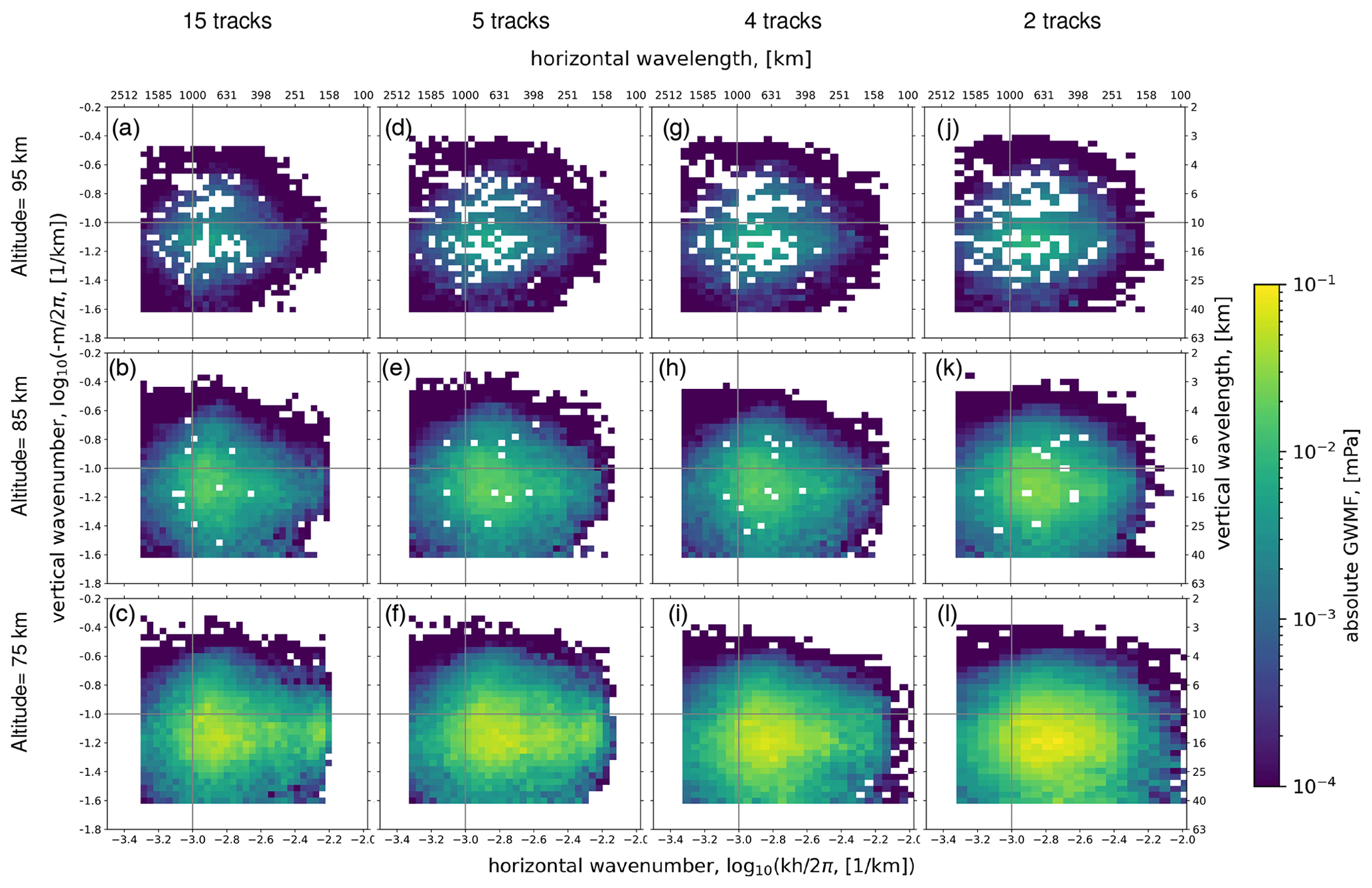
Figure 10Distribution spectra of GW pseudomomentum flux versus logarithmic horizontal and vertical wavenumbers at 75 km (bottom panels), 85 km (middle panels), and 95 km (upper panels) altitude. Varying cube sizes in the across-track direction of 15 tracks (a–c), 5 tracks (d–f), 4 tracks (g–i), and 2 tracks (j–l) are applied. The 15- and 5-track analyses are for sampled data, while 4- and 2-track analyses are for retrieval data with realistic noise. Flagged-out data due to insufficient fitting quality result in more blank bins for 95 km altitude. The gray reference lines through the plots indicate 1000 km horizontal and 10 km vertical wavelength, respectively.
We start with what we deem a good initial value for the cube size: from the HIAMCM set-up the shortest horizontal wavelength is around 156 km, and because from the observational filter of a limb sounder GWs only with horizontal wavelengths longer than 100 km are captured, we expect the shortest horizontal wavelengths of O(200 km). Small-scale GWs with horizontal wavelengths shorter than 200 km are thus not considered here. In order to gain the full picture, satellite observations need to be combined with ground-based systems (e.g., Shiokawa et al., 2009; Nishioka et al., 2013; Chum et al., 2021) observing such shorter scales (see Sect. 5). Based on previous experience and also using a separation scale of zonal wavenumber 18, the longest wavelengths to be considered are O(2000 km). An average vertical wavelength around 12 km was found from SABER data (Ern et al., 2018) for 80 km altitude. Therefore, an initial cube size of 600 km along-track × 420 km across-track × 15 km altitude is selected for fitting the wave vectors and a reduced vertical size of 5 km for refitting the wave amplitudes. With an atm-grid sampling of 30 km × 30 km × 1 km (along-track × across-track × vertical; see Sect. 3.6), this corresponds to 21 × 15 × 15 points. Spectra in terms of horizontal and vertical wavelengths for these initial cube size are shown in Fig. 10a–c for altitudes of 75, 85, and 95 km.
The spectral peak appears at around 600 to 800 km horizontally and 10 to 16 km vertically at all altitudes. All spectra are cut off at longer wavelengths of around 2100 km horizontally and 45 km vertically as the detection upper limit. It results from the limits when filtering reliable fits, which are up to ∼ 3 times the cube size for both horizontal and vertical wavelengths. This, however, does not remove major parts of the spectrum. The spectrum is slightly truncated at shorter horizontal wavelengths around 150 km at an altitude of 75 km, which is not the case for 95 km as waves with longer wavelengths can propagate higher. These wavelength spectra confirm our expectation that, at least for the model data, the target spectral range is covered well by the selected cube size parameters.
In order to investigate the impact of fewer tracks, the number of measurement tracks is reduced in several steps. The proposed mission deploys two SHIs, both with split interferograms to provide four measurement tracks in total. The distance of the track pair from one SHI is assumed to be the distance of the geometric center of the half-interferogram (30 km). The distance between the two satellites can be adjusted by pointing. We assume a gap in the center which can be used to widen the total covered region. In order to study the influence of the gap as well, we use an equidistant sampling of five points here, as well as a four-track configuration in which the center track is not used. If only one SHI instrument were operated, only two measurement tracks would be available. In order to probe all these options, a series of S3D wave analyses were conducted with cube sizes of five, four, and two across-measurement tracks on both sampled and retrieved HIAMCM temperature residual data. The five-track case is included in the simulation and discussed here as it serves as a bridge between the odd and even tracks and offers an opportunity to examine whether the S3D analysis can be performed normally on a reduced number of tracks. The along-track and vertical sizes of the analysis cubes are kept the same, i.e., 21 points and 15 points, respectively. The initial 15-track case is used as a reference for intercomparisons. We have evaluated all cases for both sampled and E2E data, but exemplarily show 15 tracks (Fig. 10a–c) and 5 tracks (Fig. 10d–f) for sampled data and 4 tracks (Fig. 10g–i) and 2 tracks (Fig. 10j–l) for full E2E data.
All three cases of reduced track numbers display the same major patterns as the reference case. It is noted that for the three cases, the spectra also have a horizontal wavelength cutoff limited to around 2100 km in order to provide an upper limit consistent with the reference case. All distributions have their maximum in horizontal wavelength at around 700 km and extend with strong amplitudes to around 300 km. This is compliant with HIAMCM having a Nyquist wavelength of ∼ 100 km and the shortest well-resolved wavelengths of the order of 250 km. For 75 km altitude, there is a secondary peak around 150 km, still inside the Nyquist limit. The fact that the wavelength limit to the short horizontal wavelength side varies with the number of tracks (and hence cube size) is due to an implementation detail of the nested interval variational fit approach. This, however, has no influence on the spectral distribution in the main part of the spectrum. There is a general tendency for larger PGWMF with fewer tracks, which is the highest for the two-track data, which look somewhat blurred, though. In general, all track combinations are suited to recover the spectrum.
4.2.2 Analysis of phase speed and wave direction
A physically more interesting test involves spectra of PGWMF versus ground-based phase speed and direction. The direction is determined from the horizontal wave vector, the intrinsic phase speed can be calculated from the dispersion relation, and the ground-based phase speed is then calculated by Doppler-shifting the phase speed with the large-scale winds. The according PGWMF distribution is shown in Fig. 11 for latitudes of 40 to 70∘ N. The panels are shown for the same number of tracks and the same altitudes as in Fig. 10. The four cases of different track numbers show common characteristics for both the phase speed values and wave directions. At 75 km altitude there are two lobes, one towards north-northeast (NNE) and a second towards southwest (SW). Maximum phase speeds in these lobes are around 50 m s−1. In addition, there is a widespread background of waves propagating (ground-based) to the east. At 95 km altitude, all low-phase-speed waves are strongly attenuated, and the north-northwest (NNW) lobe is completely removed, presumably by critical-level filtering. The fast eastward waves now prevail. The two-track data seem to have wider spread and some additional features (e.g., fast waves to the southeast, SE) which may be misinterpretations of waves. This is more pronounced at 75 km at the lower edge of the emission layer, where the noise level is higher. In general, however, all cases reproduce the same salient features.

Figure 11Polar plots of phase speed and direction versus GW pseudomomentum flux in the northern middle and higher latitudes of 40 to 70∘ at an altitude of 75 km (bottom panels), 85 km (middle panels), and 95 km (upper panels) in line with the four cases as in Fig. 10. The direction is in azimuth angle by which 0∘ is eastward and 90∘ is northward. The white dashed radius lines indicate various phase speed values in units of meters per second (m s−1).
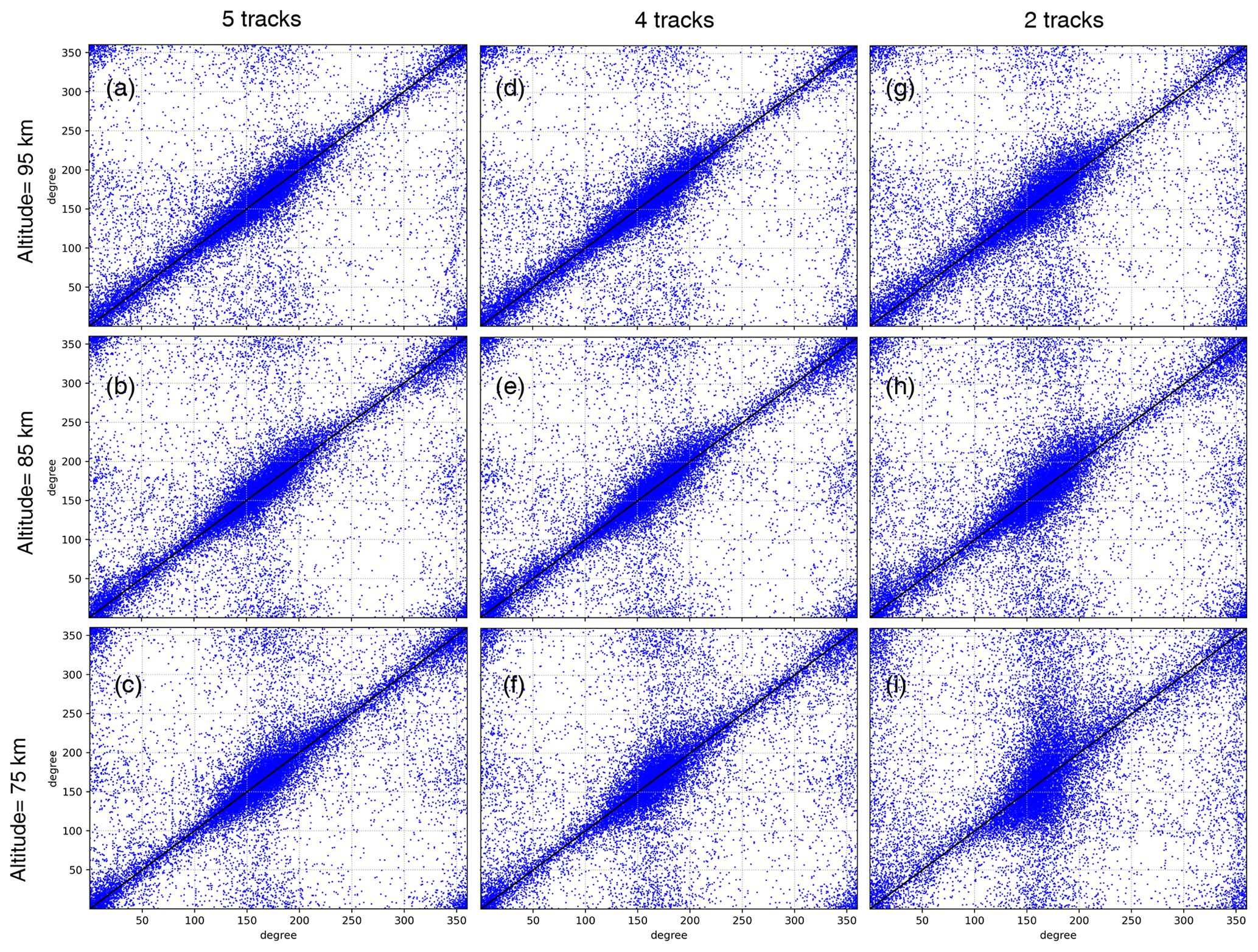
Figure 12Scatter plots of wave direction of the first wave component for 5 tracks (a–c), 4 tracks (d–f), and 2 tracks (g–i) on the y axis versus the reference of 15 tracks on the x axis at an altitude of 75 km (c, f, i), 85 km (b, e, h), and 95 km (a, d, g). A black 1 : 1 identity line is added for the comparison. Note that points around (0, 360∘) and (360, 0∘) appear simply due to a mapping of 360∘ on the y or x axis in plotting.
The deviation of wave direction caused by reducing the number of measurement tracks is further examined by scatter plots of wave directions for the various track-number cases (y axis) against the 15-track reference (x axis) in Fig. 12. The distribution is for the whole globe. We find two clusters of main propagation, a larger one around 180∘ and a smaller one around 0∘. For ideal fits, we expect identity; i.e., the same leading waves with the same wave directions would be identified independent of the number of tracks and independent of imposed noise. In this case, all points would be on the 1 : 1 identity line. Indeed, we find that most points cluster around the identity line. There are interesting deviations, though. There are smaller clusters around (0, 180∘), (180, 0∘), (360, 180∘), and (180, 360∘), which indicate direction flips. The number of direction flips increases with fewer tracks. For the two-track data there is a general loss of ability to determine the propagation direction, which is expressed in vertical stripes around the preferred propagation direction centers. Again, the loss of direction information is most pronounced at 75 km altitude.
4.2.3 Analysis of zonal mean GW momentum flux
Zonal mean GWMF and its vertical gradient constitute the primary goal of the mission and the most stringent test we can apply in the assessment. The dynamical driving and hence the overall structure of the MLT are largely governed by acceleration of the large-scale wind due to GW dissipation. Studies of equatorial oscillations, such as mesospheric semiannual oscillation (MSAO) and mesospheric quasi-biennial oscillation (MQBO), of the general mean circulation and the temperature structure as well as of the formation of an elevated stratopause after a sudden stratospheric warming are largely based on zonal mean GW activity and would highly benefit from accurate PGWMF estimates. This is further explicated is Sect. 5. Furthermore, zonal mean GWMF can be inferred as a true reference from the winds directly as introduced in Sect. 2. We discuss the influence of the observation method on this primary observation aim.

Figure 13Zonal (a–d) and meridional (f–i) zonal mean GW momentum flux in 1∘ latitude bins from sampled and retrieved orbit-track HIAMCM temperature data for 1 January 2016 at 06:00 UT using the S3D fitting method and polarization relations. Four cases as in Fig. 10 are listed. GWMF values (e, j) directly inferred from wind fluctuations are also given, which are running-averaged over 5∘ latitude bins and vertically running-averaged over 5 km altitudes.
Figure 13a–d and f–i depict altitude–latitude cross-sections of the zonal average GWMF for 1 January 2016 at 06:00 UT (i.e., winter in the Northern Hemisphere and summer in the Southern Hemisphere) in 1∘ latitudinal bins for the four cases of different numbers of observation tracks. Both zonal and meridional components are given. Except for the lowermost row, GWMF is inferred from temperature residual data via S3D wave analysis and polarization relations. We use one snapshot of HIAMCM data but sample with a series of orbits corresponding to 1 week of measurements. In this way we separate sampling issues from general limitations of the method.
Global distribution of GWMF values directly inferred from wind fluctuations as in Eq. (9) is presented in Fig. 13e and j, which serves as a reference. A running average over 5∘ latitude bins and 5 km altitude bins is applied. All main structures are recovered by the simulated observations.
The main features of Fig. 13 show that GWs intrinsically propagate against the prevailing zonal wind, i.e., eastward propagation in the summer mid-mesosphere around 70 km and westward propagation in the winter hemisphere. The MLT is characterized by strong wind gradients and according wave dissipation and critical-level filtering. This is expressed by strong gradients of GWMF and the fact that the absolute values of momentum flux change by 2 orders of magnitude, and partly, in the zonal direction by a reversal of the direction of zonal GWMF. This zonal mean behavior is consistent with the phase speed spectra of Fig. 11, which show the filtering of the high-GWMF but slow westward GWs between 75 and 95 km altitude and, accordingly, prevailing fast eastward waves at 95 km altitude. This pattern is captured by all four cases of different track numbers.
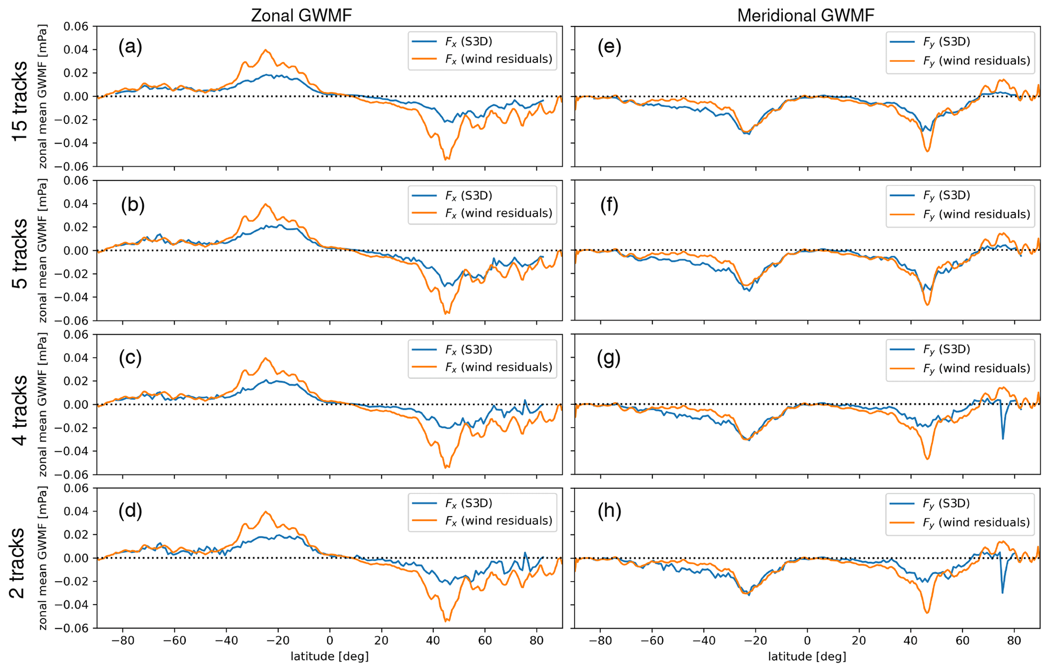
Figure 14Line comparison plots of zonal (a–d) and meridional (e–h) zonal mean GW momentum flux calculations in 1∘ latitude bins from S3D analysis (blue line) and directly from wind fluctuations (orange line) for an altitude of 75 km. It is in line with the four cases as in Fig. 10. GWMF from wind residuals is running-averaged over 5∘ latitude bins and vertically running-averaged over 5 km altitudes.
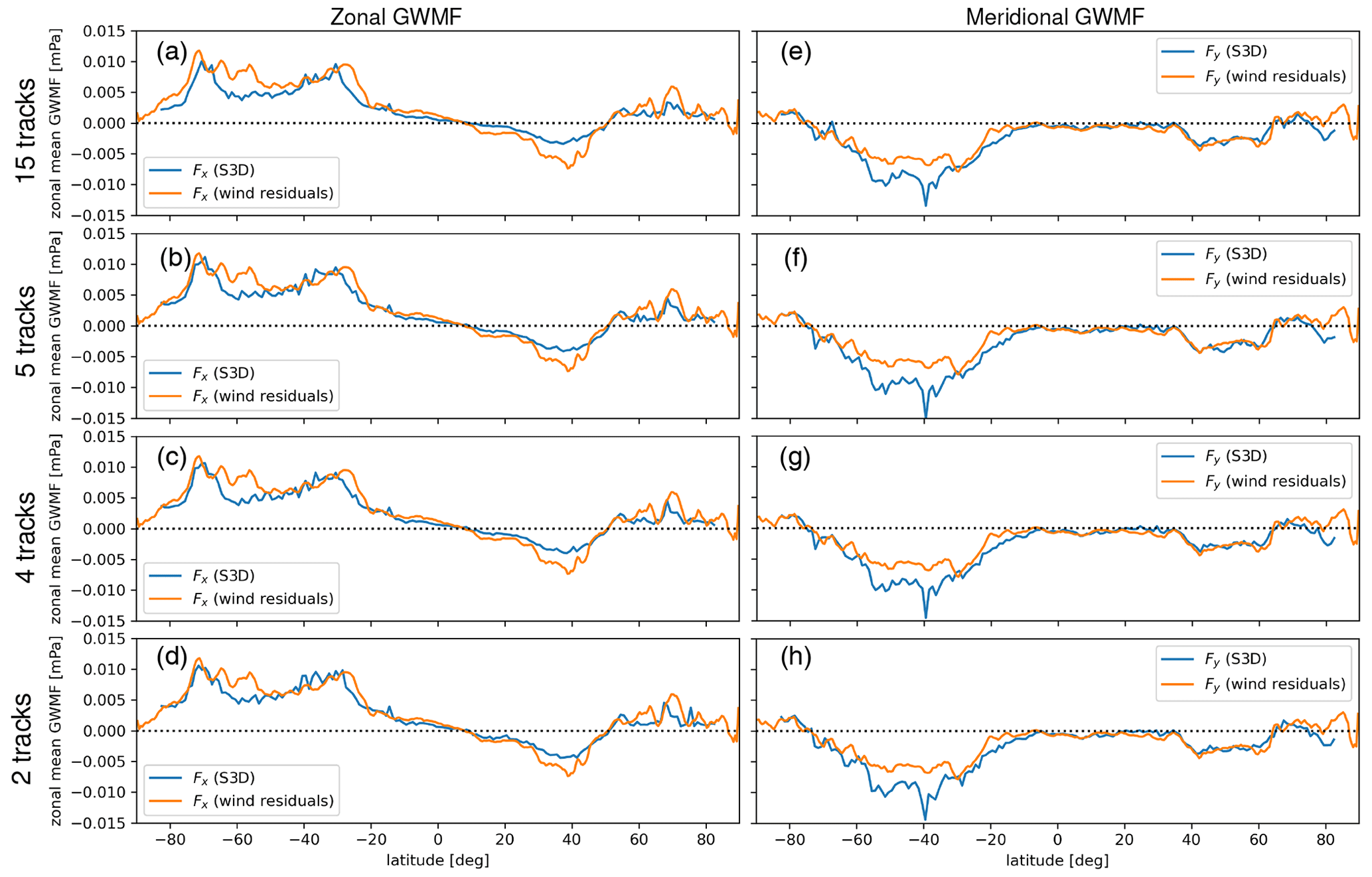
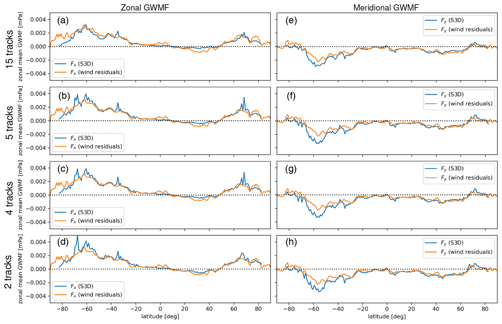
For a more quantitative comparison, line plots of momentum flux values from the four cases together with the values computed from wind residual data are presented in Figs. 14, 15, and 16 for altitudes of 75, 85, and 95 km, respectively. The line plots indicate good agreement of the momentum flux values inferred from the observed temperature residuals with the reference from model wind fluctuations. Some deviations are found in the midlatitudes for zonal GWMF components, especially at an altitude of 75 km, at 30∘ S and 40∘ N. For meridional GWMF components, discrepancies mainly appear in the Southern Hemisphere at 40–60∘ S for altitudes of 85 and 95 km. These differences are due to strong vertical gradients and could either be a problem of the wave fitting method to identify the local vertical wavelength associated with the cube center altitude or an effect of nonlinearity and limitations to the linear GW physics employed to calculate GWMF.
In conclusion, the assessment results show that wave analysis of tomographic temperature observations with few observation tracks (down to four tracks and even two tracks) is suitable to gain reliable zonal means of zonal and meridional GWMF.
4.3 How much noise can we afford?
The E2E assessment performed in Sect. 4.2 indicates the viability of the proposed mission concept based on our best estimate of instrument performance. In order to investigate whether further miniaturization of the instrument and related decrease in the signal-to-noise ratio would be feasible (see Question 3 in Fig. 2), the best-estimate noise level superposed on the synthetic spectra is scaled by multiples of 2, 4, 6, 16, and 32. After that, temperature retrieval and S3D wave analysis are performed as before. We focus on the four-track data and assess the E2E results by zonal mean zonal GWMF values (see Sect. 2.3 and the data flow to the lower yellow diamond of Question 3 in Fig. 2).
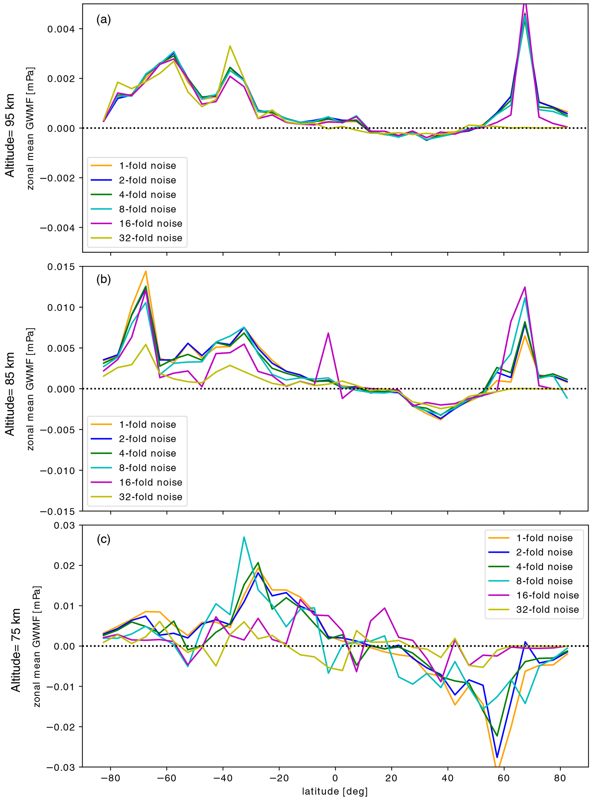
Figure 17Line plots of the zonal components of zonal mean GW momentum flux in 5∘ latitude bins from S3D analysis on retrieved temperature residuals with estimation of different noise levels of 1 (orange line), 2 (blue line), 4 (green line), 8 (cyan line), 16 (magenta line), and 32 (yellow line) at an altitude of 75 km (a), 85 km (b), and 95 km (c). A four-track case is applied for this analysis.
We show in Fig. 17 color-coded line plots for noise levels of 1, 2, 4, 8, 16, and 32 for altitudes of 75, 85, and 95 km, respectively. The resulting distributions displayed in Fig. 17 are noisier and coarser since only a single day of orbits was used. The zonal mean GWMF plots indicate that the GW structure tends to be damped with increasing noise level, but the main features are retained up to a noise level of 8 times the original. For a 32-fold noise level, the wave signals are no longer discernible. Further detailed analysis of zonal mean GWMF for a 4-fold noise level is given in Appendix C. In general, our approach could tolerate enhanced noise up to a factor of 4 higher than our best estimate of the instrument of Kaufmann et al. (2018), which allows for further downsizing of the instrument or higher detector temperatures resulting in higher dark current levels and shot noise.
Which scientific questions could be directly addressed if an instrument such that as discussed in this paper were in orbit? And for which studies would we need further ancillary data? A two-step processing chain as it would be applied to in-orbit data is sketched in Figs. 18 and 19. The first part relies only on data directly obtained by retrieval and wave analysis, and the second would involve atmospheric winds that can be calculated, e.g., by data assimilation.

Figure 18Processing chain including retrieval and GW analysis. Up to a climatology of GWMF in terms of, e.g., zonal means or monthly mean 3-D global distributions (Level 3 data) only data observed by the instrument are required.
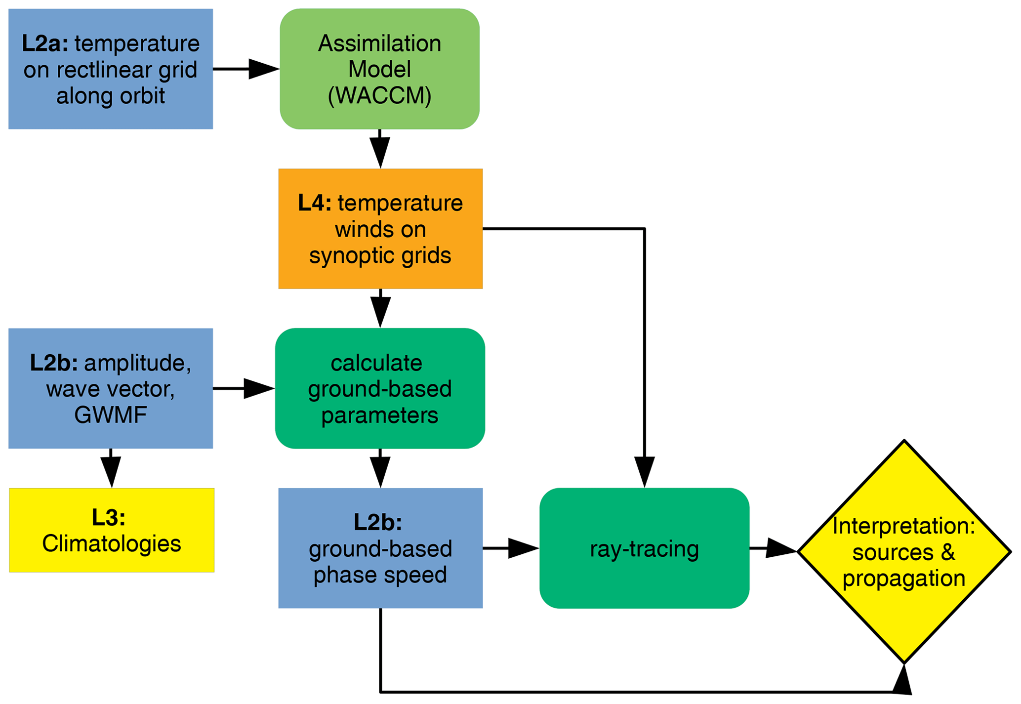
Figure 19Processing chain for scientific interpretation of propagation, source identification, and critical-level filtering. In order to determine the ground-based frequency and perform ray-tracing background wind velocities for the observation location and time are required. These can be generated as Level 4 data via assimilating various data sets (including the observations described here) in a consistent manner.
Gravity wave momentum flux can be calculated using only the observations made by the proposed instrument (Fig. 18). From the GWMF values of single GW events, climatological distributions, such as average monthly mean maps, zonal means, drag from vertical gradients of GWMF, and spectral distributions in terms of horizontal and vertical wavelength or intrinsic phase speed, can be generated. Such distributions are always the starting point of more in-depth scientific investigations and can be used for interpretations of potential sources. Together with climatologies of winds and temperatures from other observations covering the MLT altitude range (e.g., the URAP climatology; Swinbank and Ortland, 2003) they can be used to gain a first assessment of the momentum balance. Finally, spectral distributions including the direction can be used to distinguish different pathways into the MLT (as outlined in the introduction) and hence provide the information to distinguish between conceptually different modeling approaches (both GW-allowing GCMs, which still contain tunable parameters, and explicit physical GW models) better than the GW variances and absolute values of GWMF we can use nowadays.
Even more investigations are facilitated if estimates of the large-scale winds at observation time are also available. In the stratosphere such wind data are regularly generated by assimilation systems operated by numerical weather prediction centers. In the mesosphere geostrophic winds are often used, and zonal mean values were generated up to 90 km altitude (Ern et al., 2013b; Smith et al., 2017). In order to gain a 3-D and time-dependent picture including tides, data assimilation is a powerful tool (e.g., Eckermann et al., 2009; Pedatella et al., 2018, 2020).
Zonal mean winds already allow assessment of the driving of large-scale wind patterns by GWs. Examples for these are studies based on absolute values of GWMF from limb scanning. These are the most reliable estimate of global GWMF distributions we can currently gain, but they are limited because of the lack of direction information. In zones of strong vertical wind shear and an environment wherein slow-phase-speed GWs dominate, we can assume that the vertical gradient of the momentum flux corresponds to drag directed opposite to the shear (i.e., by GWs causing the shear layer to propagate downward). This concept has been very successfully used, e.g., in studies of the stratospheric quasi-biennial oscillation (Ern et al., 2014), the excitation of quasi-2 d waves (Ern et al., 2013b), and the role of GWs in sudden stratospheric warmings (Ern et al., 2016). However, in regions where substantial filtering of slower-phase-speed waves has already occurred at lower altitudes and only faster phase speeds survive or when GWs dissipate primarily due to the increasing amplitudes the waves attain when they propagate upwards into regions of lower density, such simplifications cease to work. That can be seen, for instance, in the discussion of the mesospheric semiannual oscillation (Ern et al., 2015, 2021) wherein arguments for the direction of drag became complex and indirect. This increased complexity is the mark of many of the large-scale global wind patterns in the mesosphere.
New 3-D data are a great step forward from existing observations: in the MLT region, currently existing satellite instruments do not provide 3-D information about observed GWs such that directional GWMF and directional GW drag cannot be derived. Conventional limb sounders, such as SABER or the Microwave Limb Sounder (MLS), provide only a single measurement track of altitude profiles. Accordingly, these observations are limited to GW variances (e.g., Jiang et al., 2005; Hocke et al., 2016) and GW absolute momentum fluxes (e.g., Ern et al., 2018, 2022). Solar occultations, for example by the Solar Occultation for Ice Experiment (SOFIE), are even more limited due to their sparse sampling and limited global coverage (e.g., X. Liu et al., 2014; Thurairajah et al., 2014). Other satellite instruments provide 2-D horizontal information, but GW vertical wavelengths cannot be determined (e.g., Rong et al., 2018; England et al., 2020). This means that a climatology of directional GW momentum fluxes is currently missing in the MLT region.
The proposed instrument combined with background wind information would resolve ambiguities such as those encountered by Ern et al. (2015, 2021) immediately by combining the observed GW parameters with estimates of background winds (see Fig. 19). For this, a relatively coarse spatial resolution including only wavenumbers 0–6 and a moderate altitude resolution would be sufficient. For instance, calculating the Doppler shift allows converting from intrinsic to ground-based phase speed diagrams. The ground-based phase speed spectrum could then directly be compared to the wind velocities by means of blocking diagrams as introduced by Taylor et al. (1993) and the type of GW dissipation (critical level versus saturation of growing amplitudes) inferred. The vertical gradient of the zonal or regional mean of GWMF can be used to infer net drag including its direction and taking into account GWs from all propagation directions. Also, in complex situations such as the mesospheric SAO, the contribution of GWs to the driving can be directly estimated. For such applications zonal mean winds or coarse spatial representations would suffice and a general guidance of the GCM by the assimilation system would produce novel insights.
It should be noted here that current-day assimilations still have difficulties in particularly capturing those dynamical features wherein GWs play a major role (Harvey et al., 2022a). However, when more sensors gain direction-resolved GW information, a stronger need for such fields hopefully drives improvements. The challenge in the MLT is the superposition of large-scale flow and tides, which can have similar wind amplitudes as the magnitude of the large-scale flow. However, using geostrophic winds, tidal determination from observations, and dedicated tidal models (e.g., Nguyen and Palo, 2013; Pedatella et al., 2016) there are alternatives which should also suffice for most of the investigations sketched here.
A more sophisticated way to study the interaction of GWs and large-scale winds is forward and backward ray tracing. This is more accurate than blocking diagrams as, for instance, lateral propagation and avoidance of critical levels are taken into account (Preusse et al., 2009a; Kalisch et al., 2014; Thurairajah et al., 2014; Chen et al., 2019; Thurairajah et al., 2020). Furthermore, tides, e.g., diurnal and semi-diurnal tides, cause changes in the large-scale winds at similar timescales as the periods of the GWs propagating through these winds. This causes refraction of the ground-based wave frequency (Senf and Achatz, 2011), thus also allowing waves, which would be expected to be filtered by a tide based on the original ground-based frequency at the source level, to propagate further. Having identified critical levels in backward ray tracing, however, this is a clear sign for in situ generation of GWs in the middle atmosphere by unstable jets or secondary wave generation. Also, for such studies a coarser representation of the background winds is sufficient.
Most demanding is the backward tracing of observed waves to potential tropospheric sources. Backward or forward ray tracing of individual wave events requires a full wave characterization and for temperature observations hence requires three dimensions. Backward ray tracing from 3-D data was used in previous studies for source identification. Examples for mesoscale stratospheric waves are studies by Preusse et al. (2014), Krisch et al. (2017), Perrett et al. (2021), Strube et al. (2021), and Geldenhuys et al. (2021). High-frequency waves in the MLT have also been studied by such means (Wrasse et al., 2006; Pramitha et al., 2015). Backward ray tracing is a comprehensive method to infer whether GWs can be followed down to the troposphere or meet a nontransparent level higher up – the latter indicates a source in the middle atmosphere, for instance by secondary wave generation. This is an advance over simply considering phase speeds at the observation and wind fields below as all the spatial and temporal changes in the wave parameters along the ray path are taken into account. Whether the precision of the wave parameters and the accuracy of the background winds from assimilation will be sufficient to trace mesoscale waves back to individual tropospheric sources will need to be studied in more detail. Upward ray tracing can then be used to investigate the interaction of GWs with the background and to provide a complementary drag assessment to the vertical gradient of PGWMF. For instance, which waves can reach the MLT could be assessed.
Although it is not sure whether global wind observations, or reliable winds from data assimilation, will be available in the upper mesosphere–lower thermosphere at the time the instrument will be in operation, the gravity wave data set that we expect to obtain from this novel observation method will be quite unique and of great value in itself. Even without wind observations, studies based on the observed directional gravity wave momentum flux can be performed in a climatological sense, for example by comparison with zonal wind climatologies or climatologies of atmospheric tides. Particularly, the interaction between gravity waves and tides is not well understood and offers a wide field of applications. Further, the novel gravity wave data set can be used to identify cases of excitation of secondary gravity waves. This can be performed by identifying fishbone-like structures in along-track and altitude cross-sections without the need for background wind information (e.g., Vadas et al., 2018; Vadas and Becker, 2018). For these kind of studies, the relatively short along-track sampling of 30 km, combined with a tomographic retrieval, will be very beneficial.
In the context of momentum balance studies, the observational filter of a limb sounder needs to be taken into account. The observational filter allows observing only waves with horizontal wavelengths longer than O(100 km). It is evident that this misses an important part of the GW spectrum. For instance, ground-based systems (e.g., Shiokawa et al., 2009; Nishioka et al., 2013; Chum et al., 2021) observing such shorter scales indicate large GWMF values which, upscaled to global distributions, would indicate that a larger part of the GWMF is contributed by the shorter scales. However, ground stations are situated only on land, often in hot-spot regions, rather than over open oceans, which biases the distributions. High-altitude GCMs without GW parameterization provide an argument for the importance of longer scales. They are even more restricted to long horizontal wavelengths than limb-sounding observations (e.g., Sato et al., 1999, 2012; Siskind, 2014; Becker and Vadas, 2020). It is one of the puzzles of atmospheric dynamics that these GCMs still produce a realistic atmosphere even above the stratopause where GWs become increasingly important. Further indications of the importance of scales visible to a limb sounder are the momentum budget studies discussed in the Introduction. Still, the importance of different scale GWs for the driving of the upper mesoscale is an unsolved puzzle.
For the stratosphere nowadays global simulations with a grid distance of a few kilometers and even down to 1 km are available (e.g., Stephan et al., 2019a, b; Polichtchouk et al., 2022), which allow assessment of how large a fraction of GWMF is likely to be missed due to the observational filter. However, such simulations have an upper altitude limit of less than 80 km and most of them damp GWs in a strong sponge layer above 40 km (Preusse et al., 2014, and references therein). The best estimate for such lower altitudes is that GWMF is about equally partitioned to scales shorter and longer than 100 km horizontal wavelength, respectively. The almost vanishing influence of the observational filter in our study is thus due to the fact that current state-of-the-art models do not resolve the shorter scales, and it is reasonable to assume that in reality only roughly half of the GWMF would also be observed in the mesosphere. The partitioning of momentum flux between different wavelength regions is, however, one of the major unknowns in the field of GWs, and low-error, well-characterized global observations of GWMF would be an essential and necessary step forward to answer this fundamental question. A brief outline of the current state of knowledge is given in Appendix D. In the lower thermosphere short-period, short-horizontal-wavelength GWs become strongly damped (e.g., Pitteway and Hines, 1963; Vadas, 2007; Yigit et al., 2009), and hence likely an even larger fraction of that part of the GW spectrum for which GWs can propagate upward is quantified.
The energy and momentum gravity waves deposit in the mesosphere and lower thermosphere are major drivers of the dynamics and hence the entire structure of this region. In order to understand these processes, we require global observations of gravity wave pseudomomentum flux (PGWMF), its vertical gradient, and its spectral composition. In particular, the distribution of PGWMF with respect to phase speed and direction allows direct inference of the interaction of GWs with the background winds and the mechanisms of how they drive global-scale patterns such as the general mean circulation and tropical oscillations. By observing 3-D temperature structures, one should be able to gain such information from space. The current study investigates aspects of the concrete realizations and whether it is sufficient to sample gravity waves in that part of the atmosphere with only two to four instantaneous fields of view.
To assess this question, an end-to-end simulation comprising orbit simulation, temperature retrieval, and 3-D wave analysis was performed, and the performance was assessed on the basis of GWMF comparisons. We considered zonal mean values of zonal and meridional GWMF deduced from the simulated observations and compared this to a reference distribution deduced directly from the model winds. In addition, we investigated phase speed spectra and the ability to characterize the direction of single wave events.
Our simulations show that zonal mean values are most robust and that the direction of wave events is most sensitive with respect to both noise and a low number of observation tracks. In general, a four-track instrument with nominal performance provides reliable wave quantification and can be employed for both the generation of zonal mean climatologies and studies of the interaction of GWs with the background winds.
For reasons of computational efficiency, we made the following assumptions: since the HIAMCM resolves only GWs longer than about 200 km horizontal wavelength, we have to rely on a horizontal background removal based on global-scale wave estimates. Accordingly, scale separation is not included in the assessment process. In addition, we assume a constant track distance of the split interferogram of 30 km (which implicitly assumes a constantly lit scene). Such assumptions are necessary to make the study feasible and are, on the whole, justified, but they tend to overestimate the reliability of the results somewhat. An important finding is that the signal-to-noise levels of the temperature data assumed in this study can be relaxed by a factor of 4 to allow for further miniaturization of the observation system. For the gravity wave spectrum used in this study, two fields of view parallel to the orbital track are sufficient to resolve most of the spectral distribution, whereas the direction of individual GWs cannot be resolved as well as in simulations assuming four or more tracks.
Summarizing, the most important conclusions obtained are listed below.
-
Assumptions made for the S3D fitting technique are non-critical in practical application.
-
Polarization relations are valid up to 130 km altitude.
-
Four closely spaced fields of view are sufficient to resolve the spectral distribution and the direction of gravity waves in the mesosphere. Two fields of view are sufficient to resolve the spectral distribution, but uncertainties of inferred GW direction information are increased.
-
Inferred distributions are still meaningful even if noise is increased by a factor of 4 with respect to the assumed instrument performance.
Following Sheese (2009), the A-band volume emission rate is given by
where the first term describes the production rate of the excited state , and the second term is the fraction of the O2 A band compared to all losses of the excited state . A762 is the Einstein coefficient of the A band and can be calculated by A762=FcA1Σ, where Fc is the A-band Franck–Condon factor, and A1Σ is the Einstein coefficient of all radiative transitions from the excited state corresponding to Reaction (R19) in Table A1. In the following, [⋅] corresponds to the number densities of molecules. The loss component can be calculated by
where k0, k3, k4, and k6 correspond to the quenching rates of Reactions (R20)–(R23) in Table A1. The A-band photo-absorption is calculated by
where gA is the photochemical reaction coefficient of Reaction (R1) in Table A1. The B-band photo-absorption is calculated by
where K0B, K1B, K2B, and K3B are the quenching rates of Reactions (R4)–(R7), gB is the photochemical reaction coefficient of Reaction (R2), and A771 is the Einstein coefficient of Reaction (R3) in Table A1.
Bucholtz et al. (1986)Bucholtz et al. (1986)Rothman et al. (2013)Yankovsky and Manuilova (2006)Yankovsky and Manuilova (2006)Yankovsky and Manuilova (2006)Yankovsky and Manuilova (2006)Sheese (2009)Sheese (2009)Sheese (2009)Rothman et al. (2013)Green et al. (2000)Sander et al. (2011)Sander et al. (2011)McDade et al. (1986)McDade et al. (1986)McDade et al. (1986)Nicholls (1965)Rothman et al. (2013)Sander et al. (2011)Sander et al. (2011)Sander et al. (2011)Sander et al. (2011)Table A1Photochemical reaction parameters used in the simulation of the A-band production and loss mechanisms.
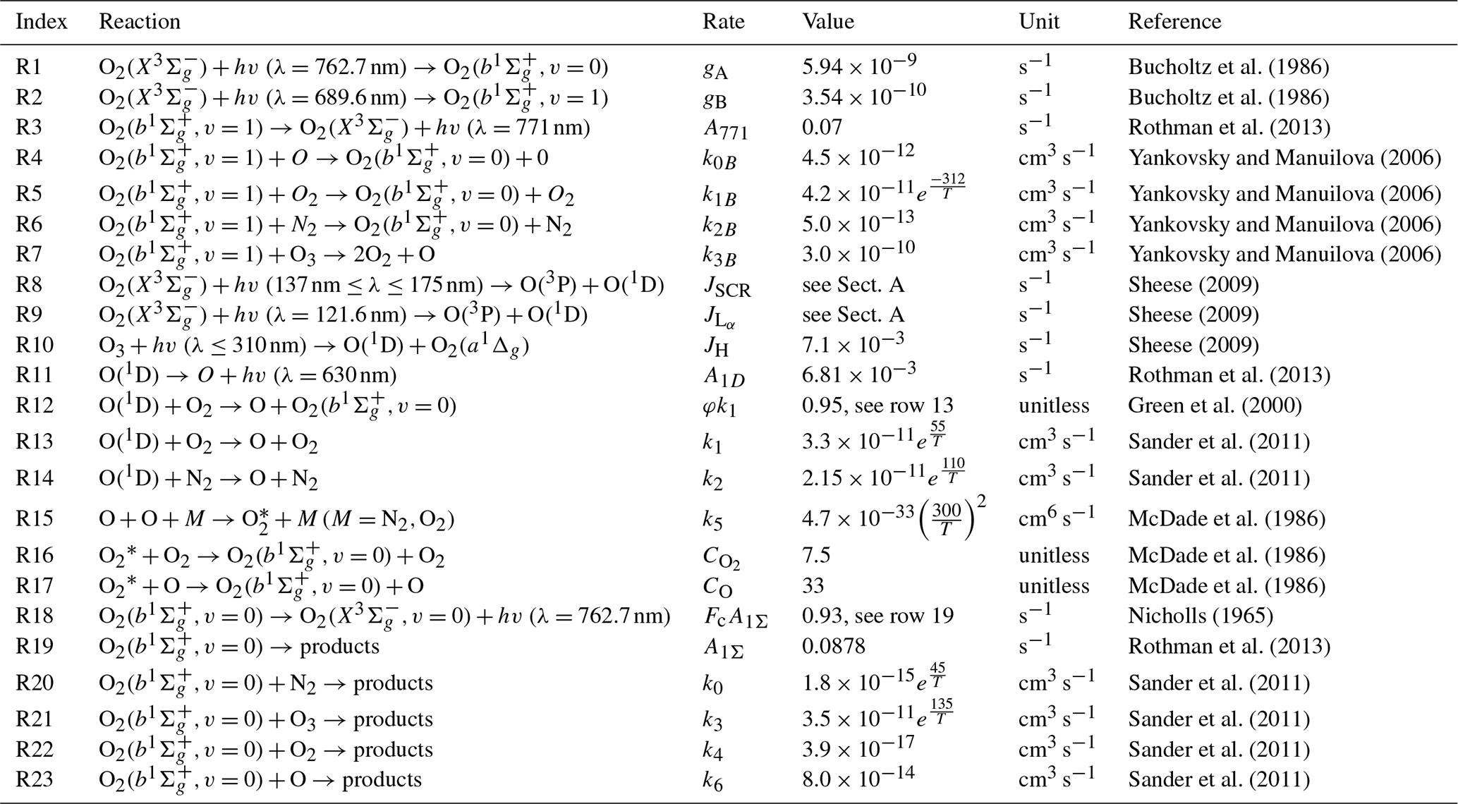
The production rate due to the photolysis of O2 and O3 can be calculated by
where JSCR, , and JH are the photolysis coefficients of Reactions (R8), (R9), and (R10), A1D is the Einstein coefficient of Reaction (R11), and k1 and k2 are the quenching rates of Reactions (R13) and (R14) in Table A1. JH is given by Sheese (2009). JSCR and are calculated by following Sheese (2009). Hereby, the Lyman-α absorption cross-section and absorption quantum yield are set to 1.0 × 10⁻²⁰ cm2 and 0.55, respectively (Reddmann and Uhl, 2003). Regarding the Schumann–Runge continuum, the absorption cross-section is given by Yoshino et al. (2005) over the given wavelength range and the absorption quantum yield is set to 1 (Brasseur and Solomon, 2005). The solar flux at the top of the atmosphere is taken from the SORCE Solar Spectral Irradiance (SSI) data product and can be obtained from https://lasp.colorado.edu/home/sorce/data/ (last access: 5 December 2022).
The production rate due to the Barth process can be calculated by
where k5 is the quenching rate of Reaction (R15) in Table A1, and and CO are the fitting parameters of the simplified model proposed by McDade et al. (1986). describes the relative quenching rates of with O2 corresponding to Reaction (R16), and CO describes the relative quenching rates of with O corresponding to Reaction (R17) in Table A1, which is a three-step reaction as depicted in Fig. 4a.
To allow for repeated tomographic retrievals of a week of data, the employed forward model makes some simplifying assumptions that need to be revisited before applying it to actual measurements. First, for daytime measurements, the model requires the amount of in-scattered solar light at all positions. This is currently being tabulated based on climatological conditions and not based on actual volume-mixing ratios. Second, the model does not take the finite extent of the line shape into account. The support of the line shape is very small compared to the spectral resolution of the instrument such that this becomes problematic only for the treatment of self-absorption: we simplify this by computing the amount of self-absorption from the center of the line, which is a strict overestimation of actual self-absorption that decreases in the line wings. In this fashion, the access to radiation from lower altitudes (below 80 km) becomes increasingly limited, which we deem a worst-case assumption for the purpose of this study; this is asserted by runs without any self-absorption that give better-quality results down to 60 km altitude. Both issues are straightforward to address by performing the required computations.
Illustrated in Fig. C1 is the global cross-section distribution of zonal mean GWMF in 1∘ latitude bins, similar to Fig. 13c of the four-track case, but for a noise level enhanced by a factor of 4. The general GW features in Fig. C1 are comparable to Fig. 13c and h, with the wind reversal and strong vertical gradients still clearly visible. In the altitude region above 80 km, these GW structures are in general well preserved in the averaged GWMF distribution, except for some outliers seen in the meridional components at 20–30∘ N for an altitude of around 85 km. Below 80 km, the latitude bins appear to be biased by noise perturbations. Particularly at 0–30∘ N and 60–40∘ S no consistent GW patterns can be identified. It reveals that the wave analysis method becomes more sensitive to noises at lower altitudes. Overall, this GWMF distribution demonstrates that our approach of wave analysis is fairly stable despite increasing the noise level by a factor of 4.
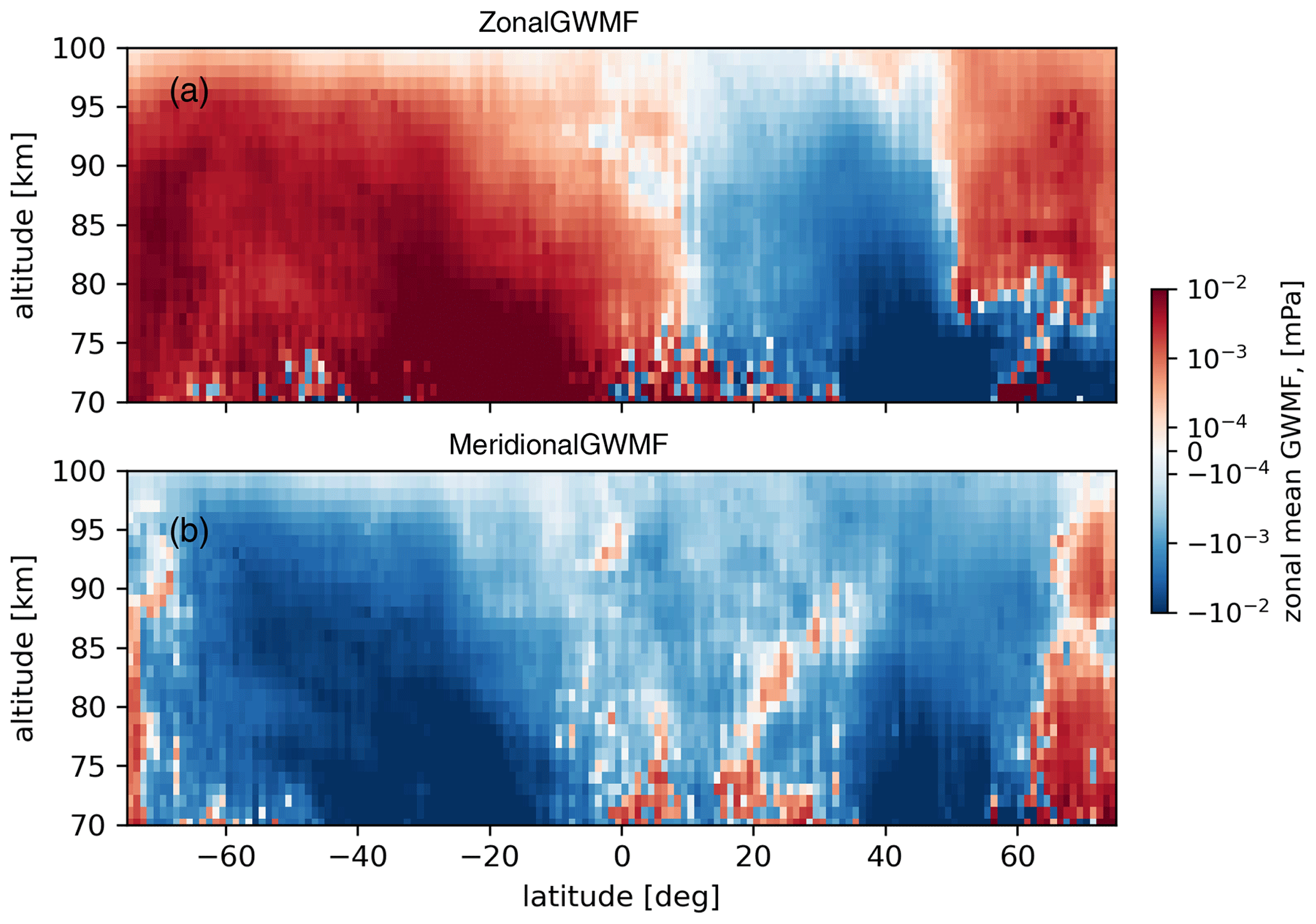
Figure C1Zonal (a) and meridional (b) components of zonal mean GW momentum flux in 1∘ latitude bins from retrieved temperature residuals with an amplified 4-fold noise level applied to a four-track case using the S3D fitting method and polarization relations.
Coupling of the different layers of the atmosphere is achieved by freely propagating (i.e., internal) GWs; other wave modes such as evanescent waves or waves in a wave guide do not contribute. This limits the horizontal range of GWs which have this potential to horizontal wavelength λh in the range of 20–30 km on the short wavelength side and to roughly 1000–2000 km on the long wavelength side (Preusse et al., 2008). Shorter wavelengths exist as well (Fritts et al., 2017), but they are important in the GW cascade when it comes to transferring momentum and energy finally to turbulence, i.e., as the last step of the cascade. A very rough first approximation of the partitioning of GWMF between different scales can be gained by assuming a universal scaling law , where the wind or temperature fluctuations scale exponentially with the horizontal wavenumber. This lets us expect that a horizontal wavelength of 100 km roughly partitions GWMF into equal parts. A detailed review by Preusse et al. (2008) found that the available evidence at the time was roughly compliant with such a partitioning. Note that here we discuss the global scale: over localized sources shorter horizontal wavelengths sometimes have larger GWMF by factors (e.g., Kruse et al., 2022), but this is then also connected to a limited area. Which evidence did we gain since the previous review of Preusse et al. (2008)? First, there are now a number of studies using the vertical derivative of absolute GWMF inferred from limb-sounding satellite instruments. It is argued in these studies that in regions of strong wind shear in particular, those GWs propagating opposite to the winds in the lower altitudes break. Despite the fact that the absolute GWMF should be underestimated by the observation technique, the contribution to the total GW acceleration expected from momentum closure is very often more than 50 % (Ern et al., 2013b, 2014, 2015, 2016). Second, we now have more model studies with GW-permitting resolution not using any GW parameterization (e.g., H. L. Liu et al., 2014; Siskind, 2014; Becker and Vadas, 2020; Okui et al., 2021; Becker et al., 2022; Okui et al., 2022). These models reach at least similar performance for the MLT and better performance for the thermosphere than GW-parameterizing GCMs as they include middle-atmosphere sources and oblique propagation, despite the fact that they resolve only GWs with horizontal wavelengths longer than ≈ 200 km. Likely, these models then somewhat overestimate the scales they resolve. Third, there are now GCM runs from numerical weather prediction (NWP) models with a much higher resolution (Stephan et al., 2019a; Polichtchouk et al., 2022). These data also indicate a roughly equal partitioning of GWMF between scales smaller and larger than a horizontal wavelength of λh = 100 km. Thus, assuming that a horizontal wavelength larger than 100 km conveys roughly half of the momentum flux is currently the best estimate we have. Unless we perform high-accuracy global GWMF observations this fundamental question will remain at least partly subject to speculation.
The code applied for this study is available from the authors on request.
The HIAMCM data are available from the authors on request. The SORCE data are freely available from the LASP-SORCE website at https://lasp.colorado.edu/home/sorce/data/ (last access: 5 December 2022; LASP, 2022).
QC performed the GW calculation as well as track- and noise-related feasibility assessment. KN was responsible for the forward model and interferogram split. BL performed the polarization relations validation. LK contributed with his knowledge about tomographic retrieval. ME was responsible for the scale separation. PP performed the orbit simulation, prepared the JUWAVE S3D software, and contributed with his expertise in GWs. PP and ME were responsible for the scientific application discussions. JU performed the tomographic temperature retrieval. EB provided the HIAMCM data and contributed to the Introduction. PP and MK initiated the topic and supervised the study. MR reviewed the paper and provided textual improvements. All authors contributed to the discussion of the results, the paper review, and improvements.
The contact author has declared that none of the authors has any competing interests.
Publisher's note: Copernicus Publications remains neutral with regard to jurisdictional claims in published maps and institutional affiliations.
We would like to acknowledge our colleague Karlheinz Nogai for his support with Fig. 1. We also thank Jaroslav Chum and one anonymous referee for their valuable comments.
This research has been partly supported by the German Ministry for Education and Research (grant no. 01 LG 1907 10, project WASCLIM) in the framework of the Role of the Middle Atmosphere in Climate (ROMIC) program.
The article processing charges for this open-access publication were covered by the Forschungszentrum Jülich.
This paper was edited by Robin Wing and reviewed by Jaroslav Chum and one anonymous referee.
Alexander, M. J.: Global and seasonal variations in three-dimensional gravity wave momentum flux from satellite limb-sounding temperatures, Geophys. Res. Lett., 42, 6860–6867, https://doi.org/10.1002/2015GL065234, 2015. a
Alexander, M. J. and Dunkerton, T. J.: A spectral parameterization of mean-flow forcing due to breaking gravity waves, J. Atmos. Sci., 56, 4167–4182, 1999. a
Alexander, M. J., Gille, J., Cavanaugh, C., Coffey, M., Craig, C., Dean, V., Eden, T., Francis, G., Halvorson, C., Hannigan, J., Khosravi, R., Kinnison, D., Lee, H., Massie, S., and Nardi, B.: Global estimates of gravity wave momentum flux from High Resolution Dynamics Limb Sounder (HIRDLS) observations, J. Geophys. Res., 113, D15S18, https://doi.org/10.1029/2007JD008807, 2008. a
Barth, C. A. and Hildebrandt, A. F.: The 5577 A airglow emission mechanism, J. Geophys. Res., 66, 985–986, https://doi.org/10.1029/JZ066i003p00985, 1961. a
Becker, E. and Vadas, S. L.: Secondary Gravity Waves in the Winter Mesosphere: Results From a High-Resolution Global Circulation Model, J. Geophys. Res.-Atmos., 123, 2605–2627, https://doi.org/10.1002/2017JD027460, 2018. a, b
Becker, E. and Vadas, S. L.: Explicit global simulation of gravity waves in the thermosphere, J. Geophys. Res.-Space, 125, e2020JA028034, https://doi.org/10.1029/2020JA028034, 2020. a, b, c, d, e, f
Becker, E., Vadas, S. L., Bossert, K., Harvey, V. L., Zülicke, C., and Hoffmann, L.: A High-Resolution Whole-Atmosphere Model With Resolved Gravity Waves and Specified Large-Scale Dynamics in the Troposphere and Stratosphere, J. Geophys. Res.-Atmos., 127, e2021JD035018, https://doi.org/10.1029/2021JD035018, 2022. a, b, c
Ben-David, A. and Ifarraguerri, A.: Computation of a spectrum from a single-beam Fourier-transform infrared interferogram, Appl. Optics, 41, 1181, https://doi.org/10.1364/AO.41.001181, 2002. a
Bertin, F., Testud, J., and Kersley, L.: Medium scale gravity waves in the ionospheric F-region and their possible origin in weather disturbances, Planet. Space Sci., 23, 493–507, 1975. a
Bossert, K., Fritts, D. C., Pautet, P.-D., Williams, B. P., Taylor, M. J., Kaifler, B., Doernbrack, A., Reid, I. M., Murphy, D. J., Spargo, A. J., and MacKinnon, A. D.: Momentum flux estimates accompanying multiscale gravity waves over Mount Cook, New Zealand, on 13 July 2014 during the DEEPWAVE campaign, J. Geophys. Res.-Atmos., 120, 9323–9337, https://doi.org/10.1002/2015JD023197, 2015. a
Bossert, K., Fritts, D. C., Heale, C. J., Eckermann, S. D., Plane, J. M. C., Snively, J. B., Williams, B. P., Reid, I. M., Murphy, D. J., Spargo, A. J., and MacKinnon, A. D.: Momentum flux spectra of a mountain wave event over New Zealand, J. Geophys. Res.-Atmos., 123, 9980–9991, https://doi.org/10.1029/2018JD028319, 2018. a
Brasseur, G. P. and Solomon, S.: Aeronomy of the middle atmosphere: chemistry and physics of the stratosphere and mesosphere, Atmospheric and oceanographic sciences library, Springer, Berlin, 3rd., rev. and enl. ed. edn., https://doi.org/10.1007/1-4020-3824-0, 2005. a
Brault, J. W.: High precision Fourier transform spectrometry: The critical role of phase corrections, Microchim. Acta, 93, 215–227, https://doi.org/10.1007/BF01201691, 1987. a
Bucholtz, A., Skinner, W. R., Abreu, V. J., and Hays, P. B.: The dayglow of the O2 atmospheric band system, Planet. Space Sci., 34, 1031–1035, https://doi.org/10.1016/0032-0633(86)90013-9, 1986. a, b, c, d
Chen, D., Strube, C., Ern, M., Preusse, P., and Riese, M.: Global analysis for periodic variations in gravity wave squared amplitudes and momentum fluxes in the middle atmosphere, Ann. Geophys., 37, 487–506, https://doi.org/10.5194/angeo-37-487-2019, 2019. a, b
Chum, J., Podolská, K., Rusz, J., Baše, J., and Tedoradze, N.: Statistical investigation of gravity wave characteristics in the ionosphere, Earth Planets Space, 73, 1–16, https://doi.org/10.1186/s40623-021-01379-3, 2021. a, b, c
Deiml, M.: Development of a small satellite remote sensing payload for passive limb sounding of the atmospheric oxygen emission, PhD thesis, University of Wuppertal, FZJ-2021-01771, https://juser.fz-juelich.de/record/891851 (last access: 5 December 2022), 2017. a
de Wit, R. J., Hibbins, R. E., Espy, P. J., Orsolini, Y. J., Limpasuvan, V., and Kinnison, D. E.: Observations of gravity wave forcing of the mesopause region during the January 2013 major Sudden Stratospheric Warming, Geophys. Res. Lett., 41, 4745–4752, https://doi.org/10.1002/2014GL060501, 2014. a
Eckermann, S. D., Hoppel, K. W., and Coy, L.: High-altitude data assimilation system experiments for the northern summer mesosphere season of 2007, J. Atm. Sol.-Terr. Phys., 71, 531–551, 2009. a
England, S. L., Greer, K. R., Solomon, S. C., Eastes, R. W., McClintock, W. E., and Burns, A. G.: Observation of thermospheric gravity waves in the Southern Hemisphere with GOLD, J. Geophys. Res. Space, 125, e2019JA027405, https://doi.org/10.1029/2019JA027405, 2020. a
Ern, M., Preusse, P., Alexander, M. J., and Warner, C. D.: Absolute values of gravity wave momentum flux derived from satellite data, J. Geophys. Res.-Atmos., 109, D20103, https://doi.org/10.1029/2004JD004752, 2004. a, b, c
Ern, M., Preusse, P., Gille, J. C., Hepplewhite, C. L., Mlynczak, M. G., Russell III, J. M., and Riese, M.: Implications for atmospheric dynamics derived from global observations of gravity wave momentum flux in stratosphere and mesosphere, J. Geophys. Res., 116, D19107, https://doi.org/10.1029/2011JD015821, 2011. a
Ern, M., Arras, C., Faber, A., Fröhlich, K., Jacobi, C., Kalisch, S., Krebsbach, M., Preusse, P., Schmidt, T., and Wickert, J.: Vertical coupling by gravity waves in atmospheric dynamics: Observations, ray tracing, and implications for global modeling, in: Climate and Waether of the Sun-Earth System (CAWSES), edited by: Lübken, F.-J., Springer Atmospheric Sciences, Dordrecht, the Netherlands, 383–408, https://doi.org/10.1007/978-94-007-4348-9, 2013a. a
Ern, M., Preusse, P., Kalisch, S., Kaufmann, M., and Riese, M.: Role of gravity waves in the forcing of quasi two-day waves in the mesosphere: An observational study, J. Geophys. Res.-Atmos., 118, 3467–3485, https://doi.org/10.1029/2012JD018208, 2013b. a, b, c
Ern, M., Ploeger, F., Preusse, P., Gille, J. C., Gray, L. J., Kalisch, S., Mlynczak, M. G., Russell III, J. M., and Riese, M.: Interaction of gravity waves with the QBO: A satellite perspective, J. Geophys. Res.-Atmos., 119, 2329–2355, https://doi.org/10.1002/2013JD020731, 2014. a, b
Ern, M., Preusse, P., and Riese, M.: Driving of the SAO by gravity waves as observed from satellite, Ann. Geophys., 33, 483–504, https://doi.org/10.5194/angeo-33-483-2015, 2015. a, b, c
Ern, M., Trinh, Q. T., Kaufmann, M., Krisch, I., Preusse, P., Ungermann, J., Zhu, Y., Gille, J. C., Mlynczak, M. G., Russell III, J. M., Schwartz, M. J., and Riese, M.: Satellite observations of middle atmosphere gravity wave absolute momentum flux and of its vertical gradient during recent stratospheric warmings, Atmos. Chem. Phys., 16, 9983–10019, https://doi.org/10.5194/acp-16-9983-2016, 2016. a, b, c, d
Ern, M., Hoffmann, L., and Preusse, P.: Directional gravity wave momentum fluxes in the stratosphere derived from high-resolution AIRS temperature data, Geophys. Res. Lett., 44, 475–485, https://doi.org/10.1002/2016GL072007, 2017. a, b
Ern, M., Trinh, Q. T., Preusse, P., Gille, J. C., Mlynczak, M. G., Russell III, J. M., and Riese, M.: GRACILE: a comprehensive climatology of atmospheric gravity wave parameters based on satellite limb soundings, Earth Syst. Sci. Data, 10, 857–892, https://doi.org/10.5194/essd-10-857-2018, 2018. a, b, c, d, e
Ern, M., Diallo, M., Preusse, P., Mlynczak, M. G., Schwartz, M. J., Wu, Q., and Riese, M.: The semiannual oscillation (SAO) in the tropical middle atmosphere and its gravity wave driving in reanalyses and satellite observations, Atmos. Chem. Phys., 21, 13763–13795, https://doi.org/10.5194/acp-21-13763-2021, 2021. a, b
Ern, M., Hoffmann, L., Rhode, S., and Preusse, P.: The mesoscale gravity wave response to the 2022 Tonga volcanic eruption: AIRS and MLS satellite observations and source backtracing, Geophys. Res. Lett., 49, e2022GL098626, https://doi.org/10.1029/2022GL098626, 2022. a
Espy, P. J., Hibbins, R. E., Swenson, G. R., Tang, J., Taylor, M. J., Riggin, D. M., and Fritts, D. C.: Regional variations of mesospheric gravity-wave momentum flux over Antarctica, Ann. Geophys., 24, 81–88, https://doi.org/10.5194/angeo-24-81-2006, 2006. a
Fetzer, E. J. and Gille, J. C.: Gravity wave variance in LIMS temperatures. Part I: Variability and comparison with background winds, J. Atmos. Sci., 51, 2461–2483, https://doi.org/10.1175/1520-0469(1994)051<2461:GWVILT>2.0.CO;2, 1994. a
Fritts, D. and Alexander, M.: Gravity wave dynamics and effects in the middle atmosphere, Rev. Geophys., 41, 1003, https://doi.org/10.1029/2001RG000106, 2003. a, b
Fritts, D. C., Wang, L., Baumgarten, G., Miller, A. D., Geller, M. A., Jones, G., Limon, M., Chapman, D., Didier, J., Kjellstrand, C. B., Araujo, D., Hillbrand, S., Korotkov, A., Tucker, G., and Vinokurov, J.: High-resolution observations and modeling of turbulence sources, structures, and intensities in the upper mesosphere, J. Atm. Sol.-Terr. Phys., 162, 57–78, https://doi.org/10.1016/j.jastp.2016.11.006, 2017. a
Geldenhuys, M., Preusse, P., Krisch, I., Zülicke, C., Ungermann, J., Ern, M., Friedl-Vallon, F., and Riese, M.: Orographically induced spontaneous imbalance within the jet causing a large-scale gravity wave event, Atmos. Chem. Phys., 21, 10393–10412, https://doi.org/10.5194/acp-21-10393-2021, 2021. a
Gisi, M., Hase, F., Dohe, S., Blumenstock, T., Simon, A., and Keens, A.: XCO2-measurements with a tabletop FTS using solar absorption spectroscopy, Atmos. Meas. Tech., 5, 2969–2980, https://doi.org/10.5194/amt-5-2969-2012, 2012. a
Green, J. G., Shi, J., and Barker, J. R.: Photochemical kinetics of vibrationally excited ozone produced in the 248 nm photolysis of O2 O3 mixtures, J. Phys. Chem. A, 104, 6218–6226, https://doi.org/10.1021/jp000635k, 2000. a
Harlander, J. M., Reynolds, R. J., and Roesler, F. L.: Spatial heterodyne spectroscopy for the exploration of diffuse interstellar emission lines at far-ultraviolet wavelengths, Astrophys. J., 396, 730–740, https://doi.org/10.1086/171756, 1992. a
Harvey, V. L., Pedatella, N., Becker, E., and Randall, C.: Evaluation of polar winter mesopause wind in WACCMX+DART, J. Geophys. Res.-Atmos., 127, e2022JD037063, https://doi.org/10.1029/2022JD037063, 2022a. a
Harvey, V. L., Pedatella, N., Becker, E., and Randall, C.: Evaluation of winter polar mesopause wind in WACCMX+DART, J. Geophys. Res.-Atmos., 127, e2022JD037063, https://doi.org/10.1029/2022JD037063, 2022b. a
Hindley, N. P., Wright, C. J., Hoffmann, L., Moffat-Griffin, T., and Mitchell, N. J.: An 18-year climatology of directional stratospheric gravity wave momentum flux from 3-D satellite observations, Geophys. Res. Lett., 47, e2020GL089557, https://doi.org/10.1029/2020GL089557, 2020. a
Hines, C. O.: Internal atmospheric gravity waves at ionospheric heights, Can. J. Phys., 38, 1441–1481, 1960. a
Hocke, K., Lainer, M., Moreira, L., Hagen, J., Fernandez Vidal, S., and Schranz, F.: Atmospheric inertia-gravity waves retrieved from level-2 data of the satellite microwave limb sounder Aura/MLS, Ann. Geophys., 34, 781–788, https://doi.org/10.5194/angeo-34-781-2016, 2016. a
Holton, J. R., Haynes, P. H., McIntyre, M. E., Douglass, A. R., Rood, R. B., and Pfister, L.: Stratosphere-Troposphere Exchange, Rev. Geophys., 33, 403–439, 1995. a
Jiang, J., Wang, B., Goya, K., Hocke, K., Eckermann, S., Ma, J., Wu, D., and Read, W.: Geographical distribution and interseasonal variability of tropical deep convection: UARS MLS observations and analyses, J. Geophys. Res.-Atmos., 109, D03111, https://doi.org/10.1029/2003JD003756, 2004. a
Jiang, J., Eckermann, S., Wu, D., Hocke, K., Wang, B., Ma, J., and Zhang, Y.: Seasonal variation of gravity wave sources from satellite observation, Adv. Space Res., 35, 1925–1932, https://doi.org/10.1016/j.asr.2005.01.099, 2005. a
Johnson, D. G., Traub, W. A., and Jucks, K. W.: Phase determination from mostly one-sided interferograms, Appl. Optics, 35, 2955–2959, https://doi.org/10.1364/AO.35.002955, 1996. a
Kalisch, S., Preusse, P., Ern, M., Eckermann, S. D., and Riese, M.: Differences in gravity wave drag between realistic oblique and assumed vertical propagation, J. Geophys. Res.-Atmos., 119, 10081–10099, https://doi.org/10.1002/2014JD021779, 2014. a
Kaufmann, M., Olschewski, F., Mantel, K., Solheim, B., Shepherd, G., Deiml, M., Liu, J., Song, R., Chen, Q., Wroblowski, O., Wei, D., Zhu, Y., Wagner, F., Loosen, F., Froehlich, D., Neubert, T., Rongen, H., Knieling, P., Toumpas, P., Shan, J., Tang, G., Koppmann, R., and Riese, M.: A highly miniaturized satellite payload based on a spatial heterodyne spectrometer for atmospheric temperature measurements in the mesosphere and lower thermosphere, Atmos. Meas. Tech., 11, 3861–3870, https://doi.org/10.5194/amt-11-3861-2018, 2018. a, b
Krall, J., Huba, J. D., Joyce, G., and Hei, M.: Simulation of the seeding of equatorial spread F by circular gravity waves, Geophys. Res. Lett., 40, 1–5, https://doi.org/10.1029/2012GL054022, 2013. a
Krisch, I., Preusse, P., Ungermann, J., Dörnbrack, A., Eckermann, S. D., Ern, M., Friedl-Vallon, F., Kaufmann, M., Oelhaf, H., Rapp, M., Strube, C., and Riese, M.: First tomographic observations of gravity waves by the infrared limb imager GLORIA, Atmos. Chem. Phys., 17, 14937–14953, https://doi.org/10.5194/acp-17-14937-2017, 2017. a
Kruse, C. G., Alexander, M. J., Hoffmann, L., van Niekerk, A., Polichtchouk, I., Bacmeister, J., Holt, L., Plougonven, R., Sacha, P., Wright, C., Sato, K., Shibuya, R., Gisinger, S., Ern, M., Meyer, C., and Stein, O.: Observed and modeled mountain waves from the surface to the mesosphere near the Drake Passage, J. Atmos. Sci., 79, 909–932, https://doi.org/10.1175/JAS-D-21-0252.1, 2022. a
LASP (Laboratory for Atmospheric and Space Physics): SOlar Radiation and Climate Experiment (SORCE) data product, Laboratory for Atmospheric and Space Physics [data set], https://lasp.colorado.edu/home/sorce/data/, last access: 5 December 2022. a
Lehmann, C. I., Kim, Y.-H., Preusse, P., Chun, H.-Y., Ern, M., and Kim, S.-Y.: Consistency between Fourier transform and small-volume few-wave decomposition for spectral and spatial variability of gravity waves above a typhoon, Atmos. Meas. Tech., 5, 1637–1651, https://doi.org/10.5194/amt-5-1637-2012, 2012. a, b
Liu, H. L.: Variability and predictability of the space environment as related to lower atmosphere forcing, Adv. Space Res., 14, 634–658, https://doi.org/10.1002/2016SW001450, 2016. a
Liu, H. L., McInerney, J. M., Santos, S., Lauritzen, P. H., Taylor, M. A., and Pedatella, N. M.: Gravity waves simulated by high-resolution Whole Atmosphere Community Climate Model, Geophys. Res. Lett., 41, 9106–9112, https://doi.org/10.1002/2014GL062468, 2014. a, b
Liu, J., Neubert, T., Froehlich, D., Knieling, P., Rongen, H., Olschewski, F., Wroblowski, O., Chen, Q., Koppmann, R., Riese, M., and Kaufmann, M.: Investigation on a SmallSat CMOS image sensor for atmospheric temperature measurement, in: International Conference on Space Optics – ICSO 2018, Chania, Greece, 9–12 October 2018, edited by: Sodnik, Z., Karafolas, N., and Cugny, B, International Society for Optics and Photonics, SPIE, vol. 11180, 2384–2393, https://doi.org/10.1117/12.2536157, 2019. a
Liu, X., Yue, J., Xu, J., Wang, L., Yuan, W., Russell III, J. M., and Hervig, M. E.: Gravity wave variations in the polar stratosphere and mesosphere from SOFIE/AIM temperature observations, J. Geophys. Res.-Atmos., 119, 7368–7381, https://doi.org/10.1002/2013JD021439, 2014. a
Marquardt, D. W.: An algorithm for least-squares estimation of nonlinear parameters, J. Soc. Ind. Appl. Math., 11, 431–441, 1963. a
McDade, I. C., Murtagh, D. P., Greer, R. G. H., Dickinson, P. H. G., Witt, G., Stegman, J., Llewellyn, E. J., Thomas, L., and Jenkins, D. B.: ETON 2: Quenching parameters for the proposed precursors of and O(1S) in the terrestrial nightglow, Planet. Space Sci., 34, 789–800, https://doi.org/10.1016/0032-0633(86)90075-9, 1986. a, b, c, d, e
McIntyre, M. E.: Breaking waves and global-scale chemical transport in the Earth's atmosphere, with spinoffs for the Sun's interior Errata, Prog. Theor. Phys., 130, 137–166, 1999. a
McLandress, C.: On the importance of gravity waves in the middle atmosphere and their parameterization in general circulation models, J. Atm. Sol.-Terr. Phys., 60, 1357–1383, https://doi.org/10.1016/S1364-6826(98)00061-3, 1998. a
Miyoshi, Y., Fujiwara, H., Jin, H., and Shinagawa, H.: A global view of gravity waves in the thermosphere simulated by a general circulation model, J. Geophys. Res. Space, 119, 5807–5820, https://doi.org/10.1002/2014JA019848, 2014. a
Nguyen, V. and Palo, S. E.: Technique to produce daily estimates of the migrating diurnal tide using TIMED/SABER and EOS Aura/MLS, J. Atm. Sol.-Terr. Phys., 105, 39–53, https://doi.org/10.1016/j.jastp.2013.07.008, 2013. a
Nicholls, R. W.: Franck-Condon Factors to High Vibrational Quantum Numbers V: O2 Band Systems, J. Res. Natl. Inst. Stand. Technol. Section A, Physics and chemistry, 69A 4, 369–373, 1965. a
Nishioka, M., Tsugawa, T., Kubota, M., and Ishii, M.: Concentric waves and short-period oscillations observed in the ionosphere after the 2013 Moore EF5 tornado, Geophys. Res. Lett., 40, 5581–5586, 2013. a, b, c
Norton, R. H. and Beer, R.: New apodizing functions for Fourier spectrometry, see errata, J. Opt. Soc. Am., 66, 259–264, 1976. a
Okui, H., Sato, K., Koshin, D., and Watanabe, S.: Formation of a mesospheric inversion layer and the subsequent elevated stratopause associated with the major stratospheric sudden warming in 2018/19, J. Geophys. Res.-Atmos., 126, e2021JD034681, https://doi.org/10.1029/2021JD034681, 2021. a
Okui, H., Sato, K., and Watanabe, S.: Contribution of gravity waves to universal vertical wavenumber (similar to m(-3)) spectra revealed by a gravity-wave-permitting general circulation model, J. Geophys. Res.-Atmos., 127, e2021JD036222, https://doi.org/10.1029/2021JD036222, 2022. a
Park, J., Lühr, H., Lee, C., Kim, Y. H., Jee, G., and Kim, J.-H.: A climatology of medium-scale gravity wave activity in the midlatitude/low-latitude daytime upper thermosphere as observed by CHAMP, J. Geophys. Res.-Space, 119, 2187–2196, https://doi.org/10.1002/2013JA019705, 2014. a
Pedatella, N. M., Oberheide, J., Sutton, E. K., Liu, H. L., Anderson, J. L., and Raeder, K.: Short-term nonmigrating tide variability in the mesosphere, thermosphere, and ionosphere, J. Geophys. Res.-Space, 121, 3621–3633, https://doi.org/10.1002/2016JA022528, 2016. a
Pedatella, N. M., Liu, H.-L., Marsh, D. R., Raeder, K., Anderson, J. L., Chau, J. L., Goncharenko, L. P., and Siddiqui, T. A.: Analysis and hindcast experiments of the 2009 sudden stratospheric warming in WACCMX+DART, J. Geophys. Res.-Space, 123, 3131–3153, https://doi.org/10.1002/2017JA025107, 2018. a
Pedatella, N. M., Anderson, J. L., Chen, C. H., Raeder, K., Liu, J., Liu, H.-L., and Lin, C. H.: Assimilation of ionosphere observations in the whole atmosphere community climate model with thermosphere-ionosphere extension (WACCMX), J. Geophys. Res.-Space, 125, e2020JA028251, https://doi.org/10.1029/2020JA028251, 2020. a
Perrett, J. A., Wright, C. J., Hindley, N. P., Hoffmann, L., Mitchell, N. J., Preusse, P., Strube, C., and Eckermann, S. D.: Determining gravity wave sources and propagation in the southern hemisphere by ray-tracing AIRS measurements, Geophys. Res. Lett., 48, e2020GL088621, https://doi.org/10.1029/2020GL088621, 2021. a, b
Pitteway, M. L. V. and Hines, C. O.: The viscous damping of atmospheric gravity waves, Can. J. Phys., 41, 1935–1948, https://doi.org/10.1139/p63-194, 1963. a
Placke, M., Hoffmann, P., Latteck, R., and Rapp, M.: Gravity wave momentum fluxes from MF and meteor radar measurements in the polar MLT region, J. Geophys. Res.-Space, 120, 736–750, https://doi.org/10.1002/2014JA020460, 2015. a
Polichtchouk, I., Wedi, N., and Kim, Y.-H.: Resolved gravity waves in the tropical stratosphere: impact of horizontal resolution and deep convection parametrization, Q. J. Roy. Meteor. Soc., 148, 233–251, https://doi.org/10.1002/qj.4202, 2022. a, b
Pramitha, M., Venkat Ratnam, M., Taori, A., Krishna Murthy, B. V., Pallamraju, D., and Vijaya Bhaskar Rao, S.: Evidence for tropospheric wind shear excitation of high-phase-speed gravity waves reaching the mesosphere using the ray-tracing technique, Atmos. Chem. Phys., 15, 2709–2721, https://doi.org/10.5194/acp-15-2709-2015, 2015. a
Preusse, P., Dörnbrack, A., Eckermann, S. D., Riese, M., Schaeler, B., Bacmeister, J. T., Broutman, D., and Grossmann, K. U.: Space-based measurements of stratospheric mountain waves by CRISTA, 1. Sensitivity, analysis method, and a case study, J. Geophys. Res., 107, CRI 6-1–CRI 6-23, https://doi.org/10.1029/2001JD000699, 2002. a
Preusse, P., Eckermann, S. D., and Ern, M.: Transparency of the atmosphere to short horizontal wavelength gravity waves, J. Geophys. Res., 113, D24104, https://doi.org/10.1029/2007JD009682, 2008. a, b, c
Preusse, P., Eckermann, S. D., Ern, M., Oberheide, J., Picard, R. H., Roble, R. G., Riese, M., Russell III, J. M., and Mlynczak, M. G.: Global ray tracing simulations of the SABER gravity wave climatology, J. Geophys. Res.-Atmos., 114, D08126, https://doi.org/10.1029/2008JD011214, 2009a. a, b, c
Preusse, P., Schroeder, S., Hoffmann, L., Ern, M., Friedl-Vallon, F., Ungermann, J., Oelhaf, H., Fischer, H., and Riese, M.: New perspectives on gravity wave remote sensing by spaceborne infrared limb imaging, Atmos. Meas. Tech., 2, 299–311, https://doi.org/10.5194/amt-2-299-2009, 2009b. a, b, c
Preusse, P., Hoffmann, L., Lehmann, C., Alexander, M. J., Broutman, D., Chun, H.-Y., Dudhia, A., Hertzog, A., Höpfner, M., Kim, Y.-H., Lahoz, W., Ma, J., Pulido, M., Riese, M., Sembhi, H., Wüst, S., Alishahi, V., Bittner, M., Ern, M., Fogli, P. G., Kim, S.-Y., Kopp, V., Lucini, M., Manzini, E., McConnell, J. C., Ruiz, J., Scheffler, G., Semeniuk, K., Sofieva, V., and Vial, F.: Observation of Gravity Waves from Space, Final report, ESA study, CN/22561/09/NL/AF, 195 pp., https://nebula.esa.int/sites/default/files/neb_study/1039/C4200022561ExS.pdf (last access: 5 December 2022), 2012. a
Preusse, P., Ern, M., Bechtold, P., Eckermann, S. D., Kalisch, S., Trinh, Q. T., and Riese, M.: Characteristics of gravity waves resolved by ECMWF, Atmos. Chem. Phys., 14, 10483–10508, https://doi.org/10.5194/acp-14-10483-2014, 2014. a, b, c
Reddmann, T. and Uhl, R.: The H Lyman-a actinic flux in the middle atmosphere, Atmos. Chem. Phys., 3, 225–231, https://doi.org/10.5194/acp-3-225-2003, 2003. a
Rodgers, C. D.: Inverse Methods for Atmospheric Sounding: Theory and Practice, vol. 2 of Series on Atmospheric, Oceanic and Planetary Physics, World Scientific, Singapore, https://doi.org/10.1142/3171, 2000. a
Roesler, F. L. and Harlander, J. M.: Spatial heterodyne spectroscopy: interferometric performance at any wavelength without scanning, in: Optical Spectroscopic Instrumentation and Techniques for the 1990s: Applications in Astronomy, Chemistry, and Physics, 1318, 234–243, https://doi.org/10.1117/12.22119, 1990. a
Rong, P., Yue, J., Russell III, J. M., Siskind, D. E., and Randall, C. E.: Universal power law of the gravity wave manifestation in the AIM CIPS polar mesospheric cloud images, Atmos. Chem. Phys., 18, 883–899, https://doi.org/10.5194/acp-18-883-2018, 2018. a
Rothman, L., Gordon, I., Babikov, Y., Barbe, A., Benner, D. C., Bernath, P., Birk, M., Bizzocchi, L., Boudon, V., Brown, L., Campargue, A., Chance, K., Cohen, E., Coudert, L., Devi, V., Drouin, B., Fayt, A., Flaud, J.-M., Gamache, R., Harrison, J., Hartmann, J.-M., Hill, C., Hodges, J., Jacquemart, D., Jolly, A., Lamouroux, J., Roy, R. L., Li, G., Long, D., Lyulin, O., Mackie, C., Massie, S., Mikhailenko, S., Müller, H., Naumenko, O., Nikitin, A., Orphal, J., Perevalov, V., Perrin, A., Polovtseva, E., Richard, C., Smith, M., Starikova, E., Sung, K., Tashkun, S., Tennyson, J., Toon, G., Tyuterev, V., and Wagner, G.: The HITRAN2012 molecular spectroscopic database, J. Quant. Spectrosc. Radiat. Transfer, 130, 4–50, https://doi.org/10.1016/j.jqsrt.2013.07.002, 2013. a, b, c
Salby, M. L.: Sampling theory for asynoptic satellite observatioons. Part I: Space-time spectra, resolution, and aliasing, J. Atmos. Sci., 39, 2577–2600, https://doi.org/10.1175/1520-0469(1982)039<2577:STFASO>2.0.CO;2, 1982. a
Sander, S., Abbatt, J., Barker, J., Burkholder, J., Friedl, R., Golden, D., Huie, R., Kurylo, M., Moortgat, G., Orkin, V., and Wine, P.: Chemical kinetics and photochemical data for use in atmospheric studies: evaluation number 17, Tech. rep., JPL Publication 10-6, Jet Propulsion Laboratory, Pasadena, http://jpldataeval.jpl.nasa.gov (last access: 5 December 2022), 2011. a, b, c, d, e, f
Sato, K., Kumakura, T., and Takahashi, M.: Gravity waves appearing in a high-resolution GCM simulation, J. Atmos. Sci., 56, 1005–1018, 1999. a
Sato, K., Tateno, S., Watanabe, S., and Kawatani: Gravity wave characteristics in the Southern Hemisphere revealed by a high-resolution middle-atmosphere general circulation model, J. Atmos. Sci., 69, 1378–1396, https://doi.org/10.1175/JAS-D-11-0101.1, 2012. a
Schmidt, H., Brasseur, G. P., Charron, M., Manzini, E., Giorgetta, M. A., Diehl, T., Fomichev, V. I., Kinnison, D., Marsh, D., and Walters, S.: The HAMMONIA Chemistry Climate Model: Sensitivity of the Mesopause Region to the 11-Year Solar Cycle and CO2 Doubling, J. Climate, 19, 3903–3931, https://doi.org/10.1175/JCLI3829.1, 2006. a, b
Senf, F. and Achatz, U.: On the impact of middle-atmosphere thermal tides on the propagation and dissipation of gravity waves, J. Geophys. Res.-Atmos., 116, D24110, https://doi.org/10.1029/2011JD015794, 2011. a
Sheese, P.: Mesospheric ozone densities retrieved from OSIRIS observations of the oxygen A-band dayglow, PhD thesis, York University, ISBN 978-0-494-64936-7, 2009. a, b, c, d, e, f, g
Shiokawa, K., Otsuka, Y., and Ogawa, T.: Propagation characteristics of nighttime mesospheric and thermospheric waves observed by optical mesosphere thermosphere imagers at middle and low latitudes, Earth Planets Space, 61, 479–491, https://doi.org/10.1186/BF03353165, 2009. a, b, c
Siskind, D. E.: Simulations of the winter stratopause and summer mesopause at varying spatial resolutions, J. Geophys. Res.-Atmos., 119, 461–470, https://doi.org/10.1002/2013JD020985, 2014. a, b
Slanger, T. G., Huestis, D. L., Osterbrock, D. E., and Fulbright, J. P.: The isotopic oxygen nightglow as viewed from Mauna Kea, Science, 277, 1485–1488, https://doi.org/10.1126/science.277.5331.1485, 1997. a, b
Smith, A. K., Garcia, R. R., Moss, A. C., and Mitchell, N. M.: The semiannual oscillation of the tropical zonal wind in the middle atmosphere derived from satellite geopotential height retrievals, J. Atmos. Sci., 74, 2413–2425, https://doi.org/10.1175/JAS-D-17-0067.1, 2017. a
Song, R., Kaufmann, M., Ungermann, J., Ern, M., Liu, G., and Riese, M.: Tomographic reconstruction of atmospheric gravity wave parameters from airglow observations, Atmos. Meas. Tech., 10, 4601–4612, https://doi.org/10.5194/amt-10-4601-2017, 2017. a
Stephan, C. C., Strube, C., Klocke, D., Ern, M., Hoffmann, L., Preusse, P., and Schmidt, H.: Gravity waves in global high-resolution simulations with explicit and parameterized convection, J. Geophys. Res.-Atmos., 124, 4446–4459, https://doi.org/10.1029/2018JD030073, 2019a. a, b
Stephan, C. C., Strube, C., Klocke, D., Ern, M., Hoffmann, L., Preusse, P., and Schmidt, H.: Intercomparison of gravity waves in global convection-permitting models, J. Atmos. Sci., 76, 2739–2759, https://doi.org/10.1175/JAS-D-19-0040.1, 2019b. a
Stober, G., Sommer, S., Rapp, M., and Latteck, R.: Investigation of gravity waves using horizontally resolved radial velocity measurements, Atmos. Meas. Tech., 6, 2893–2905, https://doi.org/10.5194/amt-6-2893-2013, 2013. a
Stober, G., Janches, D., Matthias, V., Fritts, D., Marino, J., Moffat-Griffin, T., Baumgarten, K., Lee, W., Murphy, D., Kim, Y. H., Mitchell, N., and Palo, S.: Seasonal evolution of winds, atmospheric tides, and Reynolds stress components in the Southern Hemisphere mesosphere–lower thermosphere in 2019, Ann. Geophys., 39, 1–29, https://doi.org/10.5194/angeo-39-1-2021, 2021. a
Strube, C., Ern, M., Preusse, P., and Riese, M.: Removing spurious inertial instability signals from gravity wave temperature perturbations using spectral filtering methods, Atmos. Meas. Tech., 13, 4927–4945, https://doi.org/10.5194/amt-13-4927-2020, 2020. a, b
Strube, C., Preusse, P., Ern, M., and Riese, M.: Propagation paths and source distributions of resolved gravity waves in ECMWF-IFS analysis fields around the southern polar night jet, Atmos. Chem. Phys., 21, 18641–18668, https://doi.org/10.5194/acp-21-18641-2021, 2021. a
Swinbank, R. and Ortland, D. A.: Compilation of wind data for the Upper Atmosphere Research Satellite (UARS) Reference Atmosphere Project, J. Geophys. Res.-Atmos., 108, 4615, https://doi.org/10.1029/2002JD003135, 2003. a
Tang, J., Liu, A. Z., and Swenson, G. R.: High frequency gravity waves observed in OH airglow at Starfire Optical Range NM: Seasonal variations in momentum flux, Geophys. Res. Lett., 29, 27-1–27-4, https://doi.org/10.1029/2002GL015794, 2002. a
Taylor, M. J., Ryan, E. H., Tuan, T. F., and Edwards, R.: Evidence of preferential directions for gravity wave propagation due to wind filtering in the middle atmosphere, J. Geophys. Res., 98, 6047–6057, https://doi.org/10.1029/92JA02604, 1993. a, b, c
Thurairajah, B. and Cullens, C. Y.: On the downward progression of stratospheric temperature anomalies using long-term SABER observations, J. Geophys. Res.-Atmos., 127, e2022JD036487, https://doi.org/10.1029/2022JD036487, 2022. a
Thurairajah, B., Bailey, S. M., Cullens, C. Y., Hervig, M. E., and Russell III, J. M.: Gravity wave activity during recent stratospheric sudden warming events from SOFIE temperature measurements, J. Geophys. Res.-Atmos., 119, 8091–8103, https://doi.org/10.1002/2014JD021763, 2014. a, b, c, d
Thurairajah, B., Cullens, C. Y., Siskind, D. E., Hervig, M. E., and Bailey, S. M.: The role of vertically and obliquely propagating gravity waves in influencing the polar summer mesosphere, J. Geophys. Res.-Atmos., 125, e2020JD032495, https://doi.org/10.1029/2020JD032495, 2020. a, b, c
Trinh, Q. T., Ern, M., Doornbos, E., Preusse, P., and Riese, M.: Satellite observations of middle atmosphere–thermosphere vertical coupling by gravity waves, Ann. Geophys., 36, 425–444, https://doi.org/10.5194/angeo-36-425-2018, 2018. a
Ungermann, J.: Improving retrieval quality for airborne limb sounders by horizontal regularisation, Atmos. Meas. Tech., 6, 15–32, https://doi.org/10.5194/amt-6-15-2013, 2013. a
Ungermann, J., Hoffmann, L., Preusse, P., Kaufmann, M., and Riese, M.: Tomographic retrieval approach for mesoscale gravity wave observations by the PREMIER Infrared Limb-Sounder, Atmos. Meas. Tech., 3, 339–354, https://doi.org/10.5194/amt-3-339-2010, 2010a. a, b
Ungermann, J., Kaufmann, M., Hoffmann, L., Preusse, P., Oelhaf, H., Friedl-Vallon, F., and Riese, M.: Towards a 3-D tomographic retrieval for the air-borne limb-imager GLORIA, Atmos. Meas. Tech., 3, 1647–1665, https://doi.org/10.5194/amt-3-1647-2010, 2010b. a
Ungermann, J., Blank, J., Dick, M., Ebersoldt, A., Friedl-Vallon, F., Giez, A., Guggenmoser, T., Höpfner, M., Jurkat, T., Kaufmann, M., Kaufmann, S., Kleinert, A., Krämer, M., Latzko, T., Oelhaf, H., Olchewski, F., Preusse, P., Rolf, C., Schillings, J., Suminska-Ebersoldt, O., Tan, V., Thomas, N., Voigt, C., Zahn, A., Zöger, M., and Riese, M.: Level 2 processing for the imaging Fourier transform spectrometer GLORIA: derivation and validation of temperature and trace gas volume mixing ratios from calibrated dynamics mode spectra, Atmos. Meas. Tech., 8, 2473–2489, https://doi.org/10.5194/amt-8-2473-2015, 2015. a
Vadas, S. L.: Horizontal and vertical propagation and dissipation of gravity waves in the thermosphere from lower atmospheric and thermospheric sources, J. Geophys. Res.-Space, 112, A06305, https://doi.org/10.1029/2006JA011845, 2007. a, b
Vadas, S. L. and Becker, E.: Numerical modeling of the excitation, propagation, and dissipation of primary and secondary gravity waves during wintertime at McMurdo Station in the Antarctic, J. Geophys. Res.-Atmos., 123, 9326–9369, https://doi.org/10.1029/2017JD027974, 2018. a
Vadas, S. L. and Becker, E.: Numerical modeling of the generation of tertiary gravity waves in the mesosphere and thermosphere during strong mountain wave events over the Southern Andes, J. Geophys. Res.-Space, 124, 7687–7718, https://doi.org/10.1029/2019JA026694, 2019. a, b
Vadas, S. L. and Fritts, D. C.: The Importance of spatial variability in the generation of secondary gravity waves from local body forces, Geophys. Res. Lett., 29, 45-1–45-4, https://doi.org/10.1029/2002GL015574, 2002. a
Vadas, S. L. and Fritts, D. C.: Influence of solar variability on gravity wave structure and dissipation in the thermosphere from tropospheric convection, J. Geophys. Res.-Space, 111, A10S12, https://doi.org/10.1029/2005JA011510, 2006. a
Vadas, S. L., Zhao, J., Chu, X., and Becker, E.: The Excitation of Secondary Gravity Waves from Body Forces: Theory and Observation, J. Geophys. Res.-Atmos., 123, 9296–9325, https://doi.org/10.1029/2017JD027970, 2018. a
Wrasse, C. M., Nakamura, T., Takahashi, H., Medeiros, A. F., Taylor, M. J., Gobbi, D., Denardini, C. M., Fechine, J., Buriti, R. A., Salatun, A., Suratno, Achmad, E., and Admiranto, A. G.: Mesospheric gravity waves observed near equatorial and low–middle latitude stations: wave characteristics and reverse ray tracing results, Ann. Geophys., 24, 3229–3240, https://doi.org/10.5194/angeo-24-3229-2006, 2006. a
Yankovsky, V. A. and Manuilova, R. O.: Model of daytime emissions of electronically-vibrationally excited products of O3 and O2 photolysis: application to ozone retrieval, Ann. Geophys., 24, 2823–2839, https://doi.org/10.5194/angeo-24-2823-2006, 2006. a, b, c, d
Yigit, E. and Medvedev, A. S.: Internal wave coupling processes in Earth's atmosphere, Adv. Space Res., 55, 983–1003, https://doi.org/10.1016/j.asr.2014.11.020, 2015. a
Yigit, E., Medvedev, A. S., Aylward, A. D., Hartogh, P., and Harris, M. J.: Modeling the effects of gravity wave momentum deposition on the general circulation above the turbopause, J. Geophys. Res.-Space, 114, D07101, https://doi.org/10.1029/2008JD011132, 2009. a
Yiǧit, E., Koucká Knížová, P., Georgieva, K., and Ward, W.: A review of vertical coupling in the Atmosphere–Ionosphere system: Effects of waves, sudden stratospheric warmings, space weather, and of solar activity, J. Atm. Sol.-Terr. Phys., 141, 1–12, https://doi.org/10.1016/j.jastp.2016.02.011, 2016. a, b
Yoshino, K., Parkinson, W., Ito, K., and Matsui, T.: Absolute absorption cross-section measurements of Schumann–Runge continuum of O2 at 90 and 295 K, J. Mol. Spectrosc., 229, 238–243, https://doi.org/10.1016/j.jms.2004.08.020, 2005. a
Zarboo, A., Bender, S., Burrows, J. P., Orphal, J., and Sinnhuber, M.: Retrieval of O2(1Σ) and O2(1Δ) volume emission rates in the mesosphere and lower thermosphere using SCIAMACHY MLT limb scans, Atmos. Meas. Tech., 11, 473–487, https://doi.org/10.5194/amt-11-473-2018, 2018. a
The alternative approach is to infer typical amplitudes in the MLT and request retrieval noise to be lower than a fraction of this noise. However, there is also noise suppression by regularization and by the spectral analysis software, which is difficult to estimate in a forward way in its effects on the visibility function and on the retrieved GWMF distributions.
Please note that the averaging over multiples of the wavelengths is always true in the zonal direction as this is cyclical. Therefore, the zonal GW momentum flux is always correctly evaluated. A prominent GW propagating meridionally (i.e., due south or due north), however, would be not averaged by the zonal mean per se and the phase structure should appear as a latitudinal structure. As soon as the wave possesses a notable zonal propagation component, the zonal mean will average over all phases. The meridional component of the GW momentum flux is hence also a good measure for the assessment though a less strict reference than the zonal momentum flux.
- Abstract
- Introduction
- Assessment strategy
- Models, tools, and instrument
- Assessment
- Discussion of science applications
- Conclusions
- Appendix A: Photochemical reaction parameters used in the O2 airglow emission simulation
- Appendix B: Known limitations of the O2 A-band forward model
- Appendix C: Zonal mean distribution of GWMF for a 4-fold increased noise level
- Appendix D: The relative importance of different horizontal scales
- Code availability
- Data availability
- Author contributions
- Competing interests
- Disclaimer
- Acknowledgements
- Financial support
- Review statement
- References