the Creative Commons Attribution 4.0 License.
the Creative Commons Attribution 4.0 License.
 | 13 Dec 2022
Detecting and quantifying methane emissions from oil and gas production: algorithm development with ground-truth calibration based on Sentinel-2 satellite imagery
Zhan Zhang
Evan D. Sherwin
Daniel J. Varon
Adam R. Brandt
Sentinel-2 satellite imagery has been shown by studies to be capable of detecting and quantifying methane emissions from oil and gas production. However, current methods lack performance calibration with ground-truth testing. This study developed a multi-band–multi-pass–multi-comparison-date methane retrieval algorithm that enhances Sentinel-2 sensitivity to methane plumes. The method was calibrated using data from a large-scale controlled-release test in Ehrenberg, Arizona, in fall 2021, with three algorithm parameters tuned based on the true emission rates. Tuned parameters are the pixel-level concentration upper-bound threshold during extreme value removal, the number of comparison dates, and the pixel-level methane concentration percentage threshold when determining the spatial extent of a plume. We found that a low value of the upper-bound threshold during extreme value removal can result in false negatives. A high number of comparison dates helps enhance the algorithm sensitivity to the plumes in the target date, but values in excess of 12 d are neither necessary nor computationally efficient. A high percentage threshold when determining the spatial extent of a plume helps enhance the quantification accuracy, but it may harm the yes/no detection accuracy. We found that there is a trade-off between quantification accuracy and detection accuracy. In a scenario with the highest quantification accuracy, we achieved the lowest quantification error and had zero false-positive detections; however, the algorithm missed three true plumes, which reduced the yes/no detection accuracy. In contrast, all of the true plumes were detected in the highest detection accuracy scenario, but the emission rate quantification had higher errors. We illustrated a two-step method that updates the emission rate estimates in an interim step, which improves quantification accuracy while keeping high yes/no detection accuracy. We also validated the algorithm's ability to detect true positives and true negatives in two application studies.
- Article
(9535 KB) - Full-text XML
- BibTeX
- EndNote


Methane (CH4) emissions during oil and natural gas production are receiving increased attention since CH4 is a potent greenhouse gas (GHG) with radiative forcing 84 times greater than that of CO2 over a 20-year time frame (MacKay et al., 2021). During the 2008–2017 decade, around 60 % of global methane emissions were from anthropogenic sources (Saunois et al., 2020). Of these sources, fossil fuel (coal, oil, and gas) production and use was estimated to have contributed 81–154 Tg CH4 a−1 of methane emissions, accounting for around one-third of the global anthropogenic methane fluxes (Saunois et al., 2020). Another estimate suggested that > 80 Tg of methane emissions was from the oil and gas sector across the globe in 2021, ∼ 30 % higher than the 62 Tg in 2000 (IEA, 2022). The most detailed studies to date have been performed in the United States, where the methane loss rate from oil and gas supply in 2015 was estimated at 2.3 % of the gross natural gas production (Alvarez et al., 2018). Studies also claim that the US official inventories have been consistently underestimating methane emissions in oil and natural gas systems, suggesting a more important role for methane in GHG emissions reduction in the oil and gas sector (Alvarez et al., 2018; Brandt et al., 2014; Zavala-Araiza et al., 2015; Rutherford et al., 2021).
Reducing methane loss from oil and gas systems will require measurement and monitoring. Because of the large spatial scale of the oil and gas industry, there has been significant interest in methane measurement methods using aircraft or satellites to detect methane emissions across large areas (Karion et al., 2013; Hausmann et al., 2016; Frankenberg et al., 2016; Chen et al., 2022; Cusworth et al., 2021). Satellite detection has been considered a particularly promising methane emissions monitoring technology because of its frequent revisit time, wide spatial coverage, and low labor cost. SCIAMACHY (2003–2012) and the Greenhouse Gases Observing Satellite (GOSAT, 2009–present) were the first two satellites to measure total methane columns by solar backscatter in the shortwave infrared (SWIR) (Jacob et al., 2016). The EO-1 Hyperion spectrometer achieved the first orbital detection of a methane superemitter plume from the Aliso Canyon release in 2016 (Thompson et al., 2016). The TROPOspheric Monitoring Instrument (TROPOMI) on the Sentinel-5 Precursor satellite (launched in 2017) maps methane columns with daily global coverage at up to 7 × 5.5 km2 resolution (Veefkind et al., 2012; Hu et al., 2018). The GHGSAT constellation instruments, launched from 2016 to 2022, each provide methane measurements with 25–50 m spatial resolution over a ∼ 12 × 12 km2 domain (Varon et al., 2018, 2020). More recently, the Sentinel-2 twin land-surveying satellites launched in 2015 and 2017 were shown to have moderate sensitivity to methane at specific wavelength bands (Varon et al., 2021). Other space-based sensors designed for land surface monitoring, such as PRISMA (30 m spatial resolution), Landsat-8 (30 m spatial resolution), and WorldView-3 (WV-3, 3.7 m spatial resolution), have similarly demonstrated methane detection capabilities (Cusworth et al., 2019; Ehret et al., 2022; Sánchez-García et al., 2022). Several studies in the last few years have reported methane enhancements from oil- and gas-producing regions and monitored methane “ultra-emitters” from oil and gas production based on the data from these satellite instruments (Lauvaux et al., 2022; Ehret et al., 2022; Irakulis-Loitxate et al., 2022; Cusworth et al., 2021).
The Sentinel-2 constellation has two polar-orbiting satellites placed in the same sun-synchronous orbit and phased at 180∘ to each other. The main Sentinel-2 data products are imagery from 13 spectral bands from the visible to the SWIR (Phiri et al., 2020). Among these spectral bands, bands 11 (∼ 1560–1660 nm) and 12 (∼ 2090–2290 nm) integrate radiances over methane's 1650 and 2300 nm SWIR absorption features, thus enabling methane detection and quantification. Because of its global coverage, fine spatial resolution (20 × 20 m2 in band 11 and 12), and frequent revisit time (2–5 d), Sentinel-2 is believed to have potential for large-scale high-frequency monitoring of methane plumes in oil and gas producing regions (Ehret et al., 2022).
Varon et al. (2021) developed three retrieval approaches to derive methane enhancements across a scene of a methane point source based on the Sentinel-2 data in bands 11 and 12. The single-band–multi-pass (SBMP) retrieval method uses the changes in band 12 reflectance between a satellite pass with a plume and a pass sampling a reference scene with no plume to derive methane column enhancements. The multi-band–single-pass (MBSP) retrieval compares reflectance in band 11 and 12 on a single pass. The multi-band–multi-pass (MBMP) retrieval applies two MBSP retrievals on two satellite passes to remove artifacts from the retrieval field. In that work, two case studies of applying these approaches to methane point-source plume detection from oil and gas facilities were presented, one in the Hassi Messaoud oil field of Algeria and the other in the Korpezhe oil and gas field of Turkmenistan. The Korpezhe retrieval results were shown to be consistent with GHGSAT-D satellite instrument observations in 2018–2019, albeit with higher observation density. Among the three retrieval methods, the MBMP method generally performs the best, mainly because it increases the contrast of the plumes by combining two spectral bands and having one pass sampling a reference scene.
However, the retrieval methods from Varon et al. (2021) might still be improved. First, calibration of the retrieved emission source rates with ground-truth values needs to be done to validate the performance of the sensor and the retrieval method. Varon et al. (2021) validated the retrieval results by comparing them with GHGSAT observations since GHGSAT has relatively higher precision; however, ground-truth calibration with controlled-release volumes is still essential in performance validation retrieval method fine tuning. Second, the retrieval methods include tunable parameters such as the percentage threshold during plume mask extraction. Nevertheless, the optimal values of the tunable parameters were not discussed. Lastly, because of Sentinel-2's limited sensitivity to methane, the MBMP retrieval method can generate false detections if the atmospheric conditions between satellite passes are different or if some ground features have higher reflectance in band 11 than band 12. Removing these false detections still relies on manual verification, such as checking if a similar shape occurs in the satellite observation of the other bands or in the imagery basemap. New modifications need to be made to remove the false detections at scale in a reasonable and convenient way.
Here we present a multi-band–multi-pass–multi-comparison-date (MBPD) retrieval algorithm based on the MBMP approach from Varon et al. (2021). The new algorithm extends the MBMP approach to enhance its sensitivity to methane plumes and reduces false detections. Additionally, we were able to calibrate the method using data from a single-blind controlled release in Ehrenberg, Arizona, in fall 2021. During calibration, three algorithm parameters were tuned based on the ground-truth emission rates to improve the algorithm performance. Furthermore, we show two simple application studies of the new algorithm, one examining the ability of true positive detection, and the other examining the ability of true negative detection. To our knowledge, this is the first time that a methane detection and quantification algorithm based on Sentinel-2 imagery has been calibrated with ground-truth emission rates.
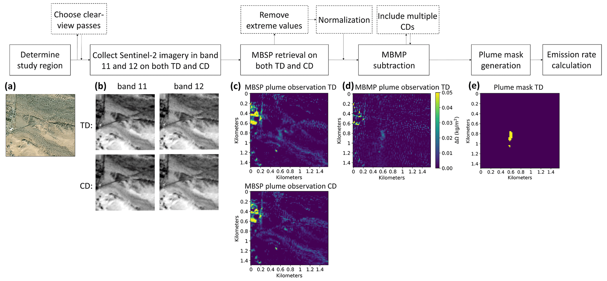
Figure 1Basic algorithm workflow. Solid boxes are specific steps of the multi-band–multi-pass (MBMP) retrieval. Dashed boxes are new modifications added in this study. (a) Study region. (b) Sentinel-2 imagery in band 11 and 12 on both target date (TD, top row) and comparison date (CD, bottom row), with pixel value as reflectance. (c) MBSP retrieval on both TD (top row) and CD (bottom row) with pixel value as methane column concentration (kg m−2). (d) MBMP retrieval on TD, i.e., the result of subtracting the MBSP retrieval on TD by the MBSP retrieval on CD. (e) Boolean plume mask generated from MBMP retrieval by selecting methane columns above some percentage threshold for the scene and smoothing with a median filter (window size 3 × 3) and a Gaussian filter (window size 3 × 3). The basemap of (a) is the ArcGIS Online World Imagery Basemap. The sources for the data used are as follows: Esri, DigitalGlobe, GeoEye, i-cubed, USDA FSA, USGS, AEX, Getmapping, Aerogrid, IGN, IGP, swisstopo, and the GIS User Community.
2.1 MBPD retrieval algorithm
The MBPD retrieval algorithm is an improved retrieval method with modifications based on the MBMP retrieval method from Varon et al. (2021). The new algorithm follows the same logic of retrieving the vertical column concentrations of atmospheric methane ΔΩ (kg m−2) from Sentinel-2 SWIR reflectances. The main steps are shown in the flow chart of Fig. 1. The main idea is retrieving methane column concentrations from one spectral measurement featuring methane absorption and one not, such as two observations from different passes with or without a methane plume or two adjacent spectral bands with different methane absorption properties. For a given scene, the method compares the Sentinel-2 measurements with the top-of-atmosphere (TOA) radiance simulated by a 100-layer, clear-sky radiative transfer model at 0.02 nm spectral resolution over the band 11 and 12 wavelength ranges. The specific steps are as follows: first, in a specific pass (pass 1), the methane concentration enhancements are retrieved by minimizing the difference between the fractional change of Sentinel-2 reflectance and a fractional absorption model based on the simulated TOA radiance in bands 11 and 12; the same process is then repeated in another pass (pass 2), and the difference of these two retrieved column enhancements (two MBSP retrievals) is the MBMP methane column enhancement in pass 1 (Eq. 1). Here the subtraction between two passes aims to remove systematic errors in the MBSP retrieval due to wavelength separation between bands 11 and 12. In other words, the MBSP retrieval in pass 2 is mainly used for removing artifacts of the MBSP retrieval in pass 1. Therefore, in this paper we name pass 1 as the “target date (TD)” and pass 2 as the “comparison date (CD)” for clarification. The TD in our method is the date for which the plume size is estimated. By default the target date is here assumed to be chronologically after the comparison date, although in practice this need not be the case.
We make some modifications during the column retrieval process since the MBMP retrieval can still lead to false detections, especially in the MBMP subtraction step (Eq. 1). In theory, in the background with no methane plume, we expect the two MBSP retrievals to have similar values of methane column enhancements since they are at the same scene. However, this is not always true because (1) MBSP retrieval can be greatly affected by the atmospheric conditions such as cloud coverage, (2) the MBSP retrieval in one pass may have similar spatial distribution but with all the pixel values higher or lower than the MBSP retrieval in another pass due to differences in various atmospheric or earth properties (e.g., solar zenith angle, surface albedo) between different dates, and (3) other unpredictable random measurement errors can occur in a specific pass. Therefore, we add the following steps to further reduce the number of false detections (see Fig. 1 for sequence).
-
Choose clear-view passes. First, we only select passes with a clear view for both the target date and comparison dates since clouds can result in false detections by affecting reflectance. Here we use Sentinel-2 cloud probability, a data product created with the sentinel2-cloud-detector library, to select clear-view passes with no large cloud coverage. Specifically, we select the passes with less than 10 % cloud coverage (i.e., the area with cloud probability higher than 65 % is less than 10 % of the total area of the study region).
-
Normalization. If two MBSP retrievals of Eq. (1) have a uniform value difference in all the pixels, artifacts will still be preserved after the MBMP subtraction. We normalize both MBSP retrievals before the MBMP subtraction to maximize the effects of artifacts removal. For example, in Fig. 2, the MBMP retrievals with normalization show more plume contrast with the background compared with the ones without normalization. Some artifacts, such as the straight line in the unnormalized retrieval with 19 September 2021 as the comparison date, are also removed in the normalized retrieval. Therefore, changing MBSP retrievals to the same scale helps enhance the ability to detect true methane plumes. However, note that the resulting concentration enhancements after normalization are no longer “actual” enhancements, and thus they should not be used to calculate the emission rates. In other words, normalization is only used for detecting the plume location and shape.
-
Remove extreme values. In some cases extremely high methane column enhancements can be generated for a small number of pixels because of the appearance of random features in one of the two passes. Thus, we also remove extreme values for the two MBSP retrievals before normalization. The removal method is based on setting upper- and lower-bound thresholds, and truncating values outside the bound thresholds to the threshold values. Here we set the lower-bound threshold as 0 kg m−2, and the upper-bound threshold will be tuned using the controlled-release experimental data below. Similar to normalization, this step is only used for plume detection instead of quantification.
-
Include multiple comparison dates. Instead of using a single comparison date, we include multiple comparison dates to help with plume detection. Different from the “sliding window” method from Ehret et al. (2022), which uses a multi-linear regression onto 1–20 previous passes, we directly take the average of comparison date retrievals as the subtrahend in the MBMP subtraction. Using multiple comparison days helps to stabilize the background since the background values can vary among different passes due to weather, temperature, surface albedo difference, and other variation. Shown in Fig. 3, more comparison dates provide a more stable background and therefore are more likely to increase the contrast of the plumes. On the other hand, it is possible that in real application, the comparison date may also have methane plumes at the same location with a similar shape as the plumes in the target date. In this case, it is harder for the algorithm to detect the target date plumes after the MBMP subtraction. Therefore, using the average of multiple comparison dates helps lower the possibility of the occurrence of a high-volume methane plume in the subtrahend, thus enhancing the algorithm sensitivity to the plumes in the target date. Here the comparison dates are selected as continuous clear-view passes before the target date, and the number of comparison dates is a parameter that will be tuned using the controlled-release experimental data below. Because the new algorithm considers multiple comparison dates for the multi-band–multi-pass approach, it is named the “Multi-band–multi-pass–multi-comparison-date” (MBPD) retrieval algorithm.
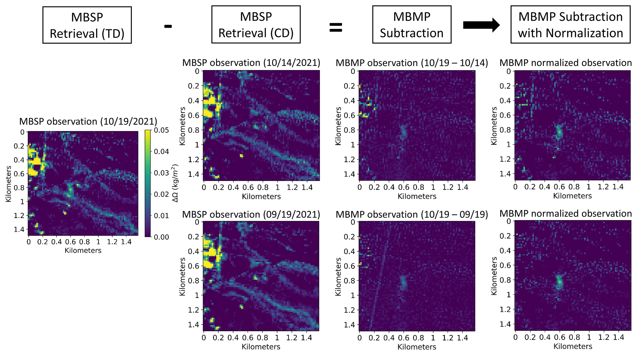
Figure 2Examples of normalization. Here are two MBMP retrieval examples, one with 19 October 2021 as target date (TD) and 14 October 2021 as comparison date (CD) and another with 19 October 2021 as TD and 10 September 2021 as CD. In each example, we show MBMP plume observation without and with normalization (see figures of the third and fourth column from left). In both examples, the normalized MBMP retrieval shows more plume contrast with the background than the one without normalization. In the second example with 10 September 2021 as CD, there is a particularly straight line artifact in the MBMP retrieval without normalization, and it is removed in the normalized MBMP retrieval. This illustrates the fact that normalization improves the effect of artifact removal by making MBSP retrievals of TD and CD conform to the same scale.
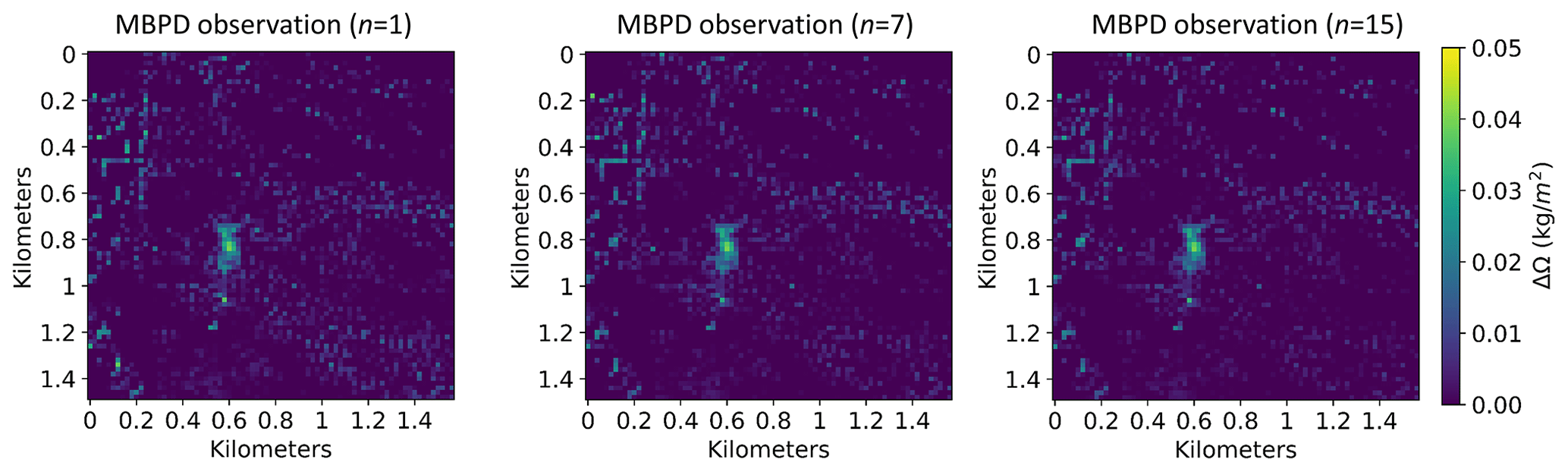
Figure 3Examples of including multiple comparison dates. In the MBMP subtraction, we include multiple comparison dates and take their average MBSP retrievals as the subtrahend to stabilize the varying background in different dates. Here n is the number of comparison dates. From left to right (n = 1, 7, and 15, respectively), we can see that a higher n provides a “cleaner” background in the MBPD retrieval, particularly in the lower right area, and thus increases the contrast of the plume.
After column retrieval, the methane column enhancements ΔΩMBPD are further used to calculate the emission source rate Q using the integrated mass enhancement (IME) method described by Varon et al. (2021) (Eq. 2) (Frankenberg et al., 2016; Varon et al., 2018). In this equation, IME is the integrated mass enhancement (kg), Ueff is the effective wind speed (m/s), and L is the plume size (m).
To calculate IME, we first generate Boolean plume masks based on ΔΩMBPD by selecting methane columns above some percentage threshold for the scene and smooth with a 3 × 3 median filter and a 3 × 3 Gaussian filter (see Fig. 1e). Here the percentage threshold is a parameter that will be tuned using the controlled-release experimental data below. This plume mask generation step sets the location and shape of the methane plumes.
Then the IME is defined as the sum of multiplication of column enhancements and pixel-level area of all the mask pixels. Note that the column enhancements here are the original enhancements without any data transformation such as normalization or extreme value removal applied to aid detection of the plume shape. The effective wind speed Ueff is the function of the local 10 m wind speed U10 derived by Varon et al. (2021), calibrated with large-eddy simulations. We collect local wind speed data from the high-resolution rapid refresh (HRRR) atmospheric model from the US National Oceanic and Atmospheric Administration (US NOAA, 2021). The plume size L is taken in a simplified form as the square root of the plume mask area.
2.2 Performance assessment
To validate the performance of the new algorithm, calibration is required to compare the algorithm outcome with the ground truth. The goal of calibration is to assess the algorithm performance in both detection and quantification. Accurate yes/no detection is defined as the algorithm being able to detect a methane plume when it appears and detecting nothing when no plume appears. Accurate quantification means that the emission rate estimates derived from the algorithm are consistent with the ground-truth measured release volumes.
Additionally, the algorithm performance can also be improved by parameter tuning to best match the ground truth. Here the following three parameters in the new algorithm are tuned: (1) the upper bound threshold during extreme value removal bu, (2) the number of comparison dates for each target date n, and (3) the percentage threshold during the plume mask generation p. The way each parameter affects the algorithm outcome is described as follows.
-
The upper-bound threshold bu. bu is a parameter that occurs during the extreme value removal, during which the retrieval values higher than it are considered to be extreme outliers and are replaced by the threshold value. Thus, a lower bu means a more strict constraint during extreme value removal. Ideally, an optimal bu helps remove false detections due to the extreme highs. However, if bu is too low, a true methane plume may also be ignored since its retrieval values could be removed.
-
The number of comparison dates n. We expect that the higher n is, the more stable the background is, thus the contrast of the plume is increased. However, this stability increase is not linear, so the increase in n may not help much in the case of a very large n. In addition, the computation workload also increases along with higher n, approximately linearly with n.
-
The percentage threshold p. The higher p is, the fewer pixels are included in the plume mask. Thus, a higher p means a smaller plume mask area. This may help with removing false positives and enhancing quantification accuracy, but may also lead to false negatives or result in underestimation of plume volume if selected at too high of a value.
To quantify the algorithm performance, we use two assessment factors with focus on different aspects. First, we choose F1 score to assess the performance of detection. F1 score is a function of “precision” and “recall”, measures of false positives and false negatives, respectively (Eqs. 3–5). F1 score has a range of 0 to 1, with higher values representing better algorithm performance. In addition, we choose the average absolute error (AAE) to assess the performance of quantification (Eq. 6, where xi and are the emission rate estimate and ground-truth emission rate in day i, and N is the number of days). AAE has a range of 0 to ∞ with lower values suggesting better algorithm performance. Absolute error is used so that under- and over-estimates do not cancel each other out.
In fall 2021, a single-blind controlled-release test was conducted by the Stanford University Environmental Assessment & Optimization Group. The test was performed in Ehrenberg, Arizona, the testing methods are described in detail in Sherwin et al. (2021) and Rutherford et al. (2022), and the test was generally similar to previous tests of airplane-based methane plume detection from the same group (Sherwin et al., 2021). This test aimed at assessing the performance of various aircraft and satellite methane detection technologies. During the test, the participants were given the information of time and location of the potential release, although the methane plume volumes (including zero, i.e., no methane plume) were unknown to them. Participants were asked to estimate the mass emissions rate during each observation (in kg CH4 h−1). Specifically for Sentinel-2, there are seven clear-view satellite passes and one cloud-covered pass covered in this test from 17 October 2021 to 3 November 2021. Here we consider only the seven clear-view passes and also add three dates after the test with zero emission, so that in total 10 target dates with ground-truth emission rates are used to do the ground-truth calibration. Of the 10 target dates, 5 have methane plumes with non-zero emission rates and 5 have no methane plumes. Region A in Fig. 4 is the study region that covers the controlled-release point source. After calibration, we also provided two simple application studies to validate the algorithm performance (Sect. 3.2). Because we lacked other ground-truth data to use as a blind test set, one goal of these application studies was to test if the algorithm can avoid generating false positives in the case of no methane plumes.
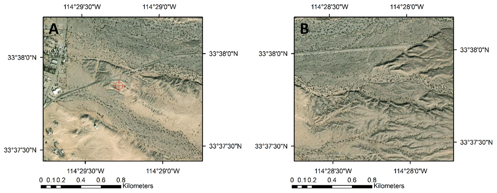
Figure 4Study regions. Region A covers the controlled-release point source (red-marked, 33.6306∘ N, 114.4878∘ W) and is mainly used for the controlled-release calibration. Region B is to the east of region A with the same area and is used for the application study. The basemap is the ArcGIS Online World Imagery Basemap. The sources for the data used are as follows: Esri, DigitalGlobe, GeoEye, i-cubed, USDA FSA, USGS, AEX, Getmapping, Aerogrid, IGN, IGP, swisstopo, and the GIS User Community.
3.1 Controlled-release calibration
We selected a wide value range for each algorithm parameter during the parameter tuning. For bu, we noticed that the magnitudes of the pixel-level column enhancements of a methane plume are usually from 10−3 to 10−1 kg m−2. Thus, we selected 10 values from 0.01 to 0.1 kg m−2 with increments of 0.01 kg m−2 and four other values 0.005, 0.12, 0.15, and 0.20 kg m−2. For n, for each target date 15 clear-view passes were selected with the earliest comparison date around 45 d before the target date, so n ranges from 1 to 15 with increments of 1. For p, 16 values were selected from 0.80 to 0.95 with increments of 0.01. Therefore, there are in total 3360 scenarios of different combinations of three parameters. Each of these 3360 parameter settings were run to quantify volumes from all 10 study days.
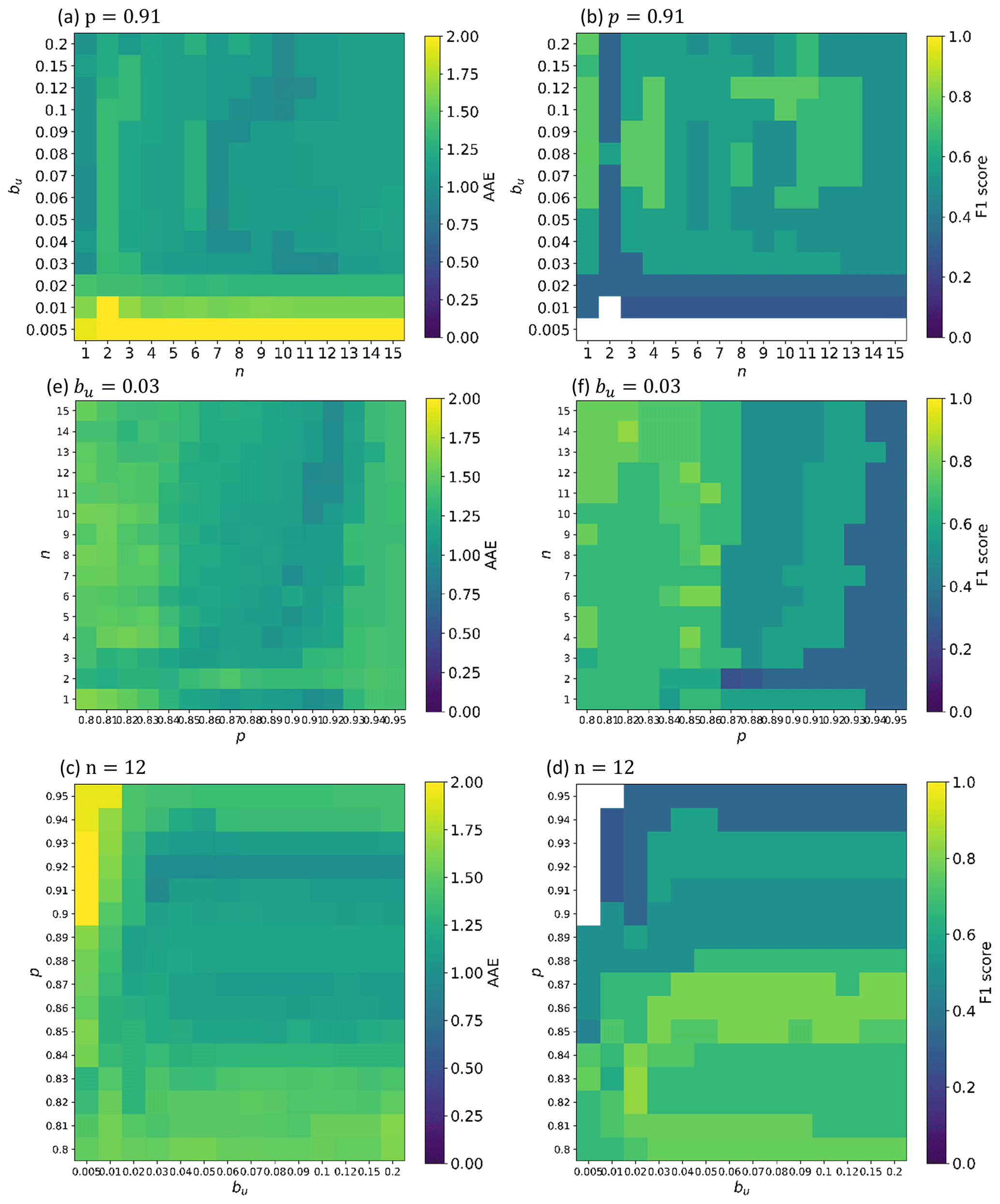
Figure 5Parameter tuning scenarios. Three algorithm parameters are tuned: the upper bound threshold during extreme value removal bu, the number of comparison dates for each target date n, and the percentage threshold during the plume mask generation p. Two assessment factors are used with focus on different aspects: the average absolute error (AAE) assesses quantification performance, and F1 score assesses detection performance. A total of 3360 parameter settings were run with wide value ranges of three parameters. Panels (a) and (b) show how AAE and F1 score change with bu and n, respectively, with p = 0.91; (c) and (d) show how two assessment factors change with n and p with bu = 0.03; (e) and (f) show how they change with p and bu with n = 12. The fixed values are from the parameter setting with the lowest AAE. White space indicates a not a number (NAN) value of F1 score resulted from zero true positive.
Figure 5 shows how each parameter affects the algorithm outcome. In each figure, an assessment factor (AAE or F1 score) is shown as a function of two parameters, based on a fixed value of the third parameter (i.e., a “slice” through 2 parameters keeping the third constant). Here the fixed values are from the parameter setting with the lowest AAE. Figure 5a and b show that a small bu value (0.005–0.02 kg m−2) leads to bad algorithm performance with high AAE and low F1 score (AAE > 1.3, F1 score < 0.4). This suggests that the bu constraint is too strict in this range and removes retrievals not only from the extreme highs but also from true methane plumes. Thus, the algorithm starts to generate false negatives. Particularly in Fig. 5b when bu is 0.005 kg m−2, we see NAN values of F1 score because there is no true positive detection at all. Aside from the low-value range, AAE and F1 score show less sensitivity to bu at the other values. Therefore, the conclusion from bu tuning is that one should avoid excessively low values of bu (< 0.02 kg m−2).
Figure 5a and c show a rough decreasing trend of AAE along with higher n when n < 12. This suggests that a higher n helps with quantification accuracy by providing a more stable background and lowering the possibility of high-volume plume in the comparison dates. However, AAE does not show an obvious decrease when n ≥ 12, which suggests that 12 or more comparison dates are not necessary or at least cease to improve performance. Figure 5b and d show low F1 scores when n is low (for example, F1 scores < 0.67 when n = 2). This is because some target dates have their earlier comparison dates with higher methane plume volumes, and a low value of n does not effectively reduce the average volume in the comparison dates, thus resulting in more false negatives. In real applications, this may be a more serious problem if the plume is continuous across a long time period with varying volumes. Additionally, computational cost is roughly proportional to n, so too high of a value of n can have excessive computational costs with little benefit to accuracy. Therefore, the value of n should not be too low or too high, and from the figures we can conclude that a reasonable choice of n is in the range 10–12.
Figure 5c and e show that AAE decreases with higher p at first but starts to increase when p > 0.92. The decreasing trend is due to smaller plume volumes and fewer false positives resulting from smaller plume masks during the Boolean plume mask generation. The increasing trend in high p range, however, is because p becomes sufficiently high such that no mask is generated even for the dates with real methane plumes. This also explains why in Fig. 5d and f that the F1 score is low in high p ranges. Low AAEs occur in the p range 0.91–0.93, while high F1 scores occur in the p range 0.85–0.86. This suggests a trade-off between accurate quantification and accurate yes/no detection: accurate quantification usually requires a high p value, but accurate yes/no detection needs a lower p value (though not excessively low). Therefore, when selecting the best p value, we can choose to emphasize quantification accuracy and accept the possibility of missing plumes (p > 0.90), or we can choose to detect more plumes and accept the possibility of emission rate overestimation (p ≈ 0.85).
Table 1Scenario examples of three parameters.
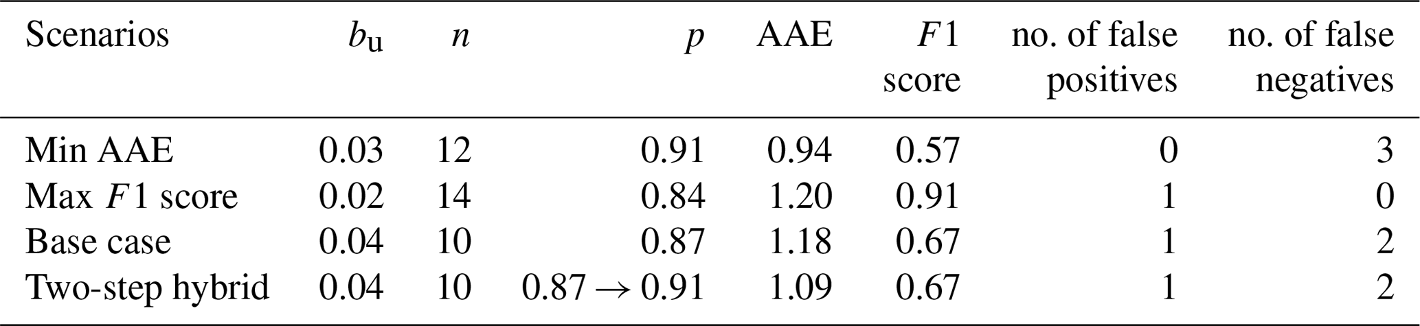
“Min AAE” scenario is the scenario with the lowest AAE, “max F1 score” scenario is the scenario with the highest F1 score; “base case” scenario is the base case of the two-step application method example, “two-step hybrid” scenario is the two-step application method example.
Table 2Emission rate estimates of scenario examples.
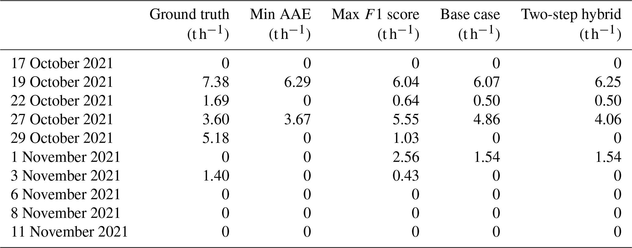
“Min AAE” scenario is the scenario with the lowest AAE, “max F1 score” scenario is the scenario with the highest F1 score, “base case” scenario is the base case of the two-step application method example, “two-step hybrid” scenario is the two-step application method example.
Here two specific scenarios shown in Tables 1 and 2 further illustrate the trade-off between accurate quantification and accurate yes/no detection. The “min AAE” scenario is an example of pursuing quantification accuracy. It has the lowest AAE of all the parameter settings and the highest precision, meaning that it also has the minimum amount of false positives. However, this scenario has three false negatives that reduce the F1 score. Aside from this specific scenario, the top 1 % scenarios with low AAEs have their bu ranging widely at 0.03–0.15, n in a middle-to-high range of 7–14, and p staying high at 0.91–0.92. On the other hand, the “max F1 score” scenario has the highest F1 score. It does not have false negatives, but in order to find all plumes it becomes too aggressive, leading to one false positive. Note that multiple scenarios have the same highest F1 score, and the scenario we show here is the one with the lowest AAE among them. The top 1 % scenarios with high F1 scores have their bu ranging widely at 0.02–0.12, n in a wide range of 1–15, and p in the middle range of 0.82–0.85.
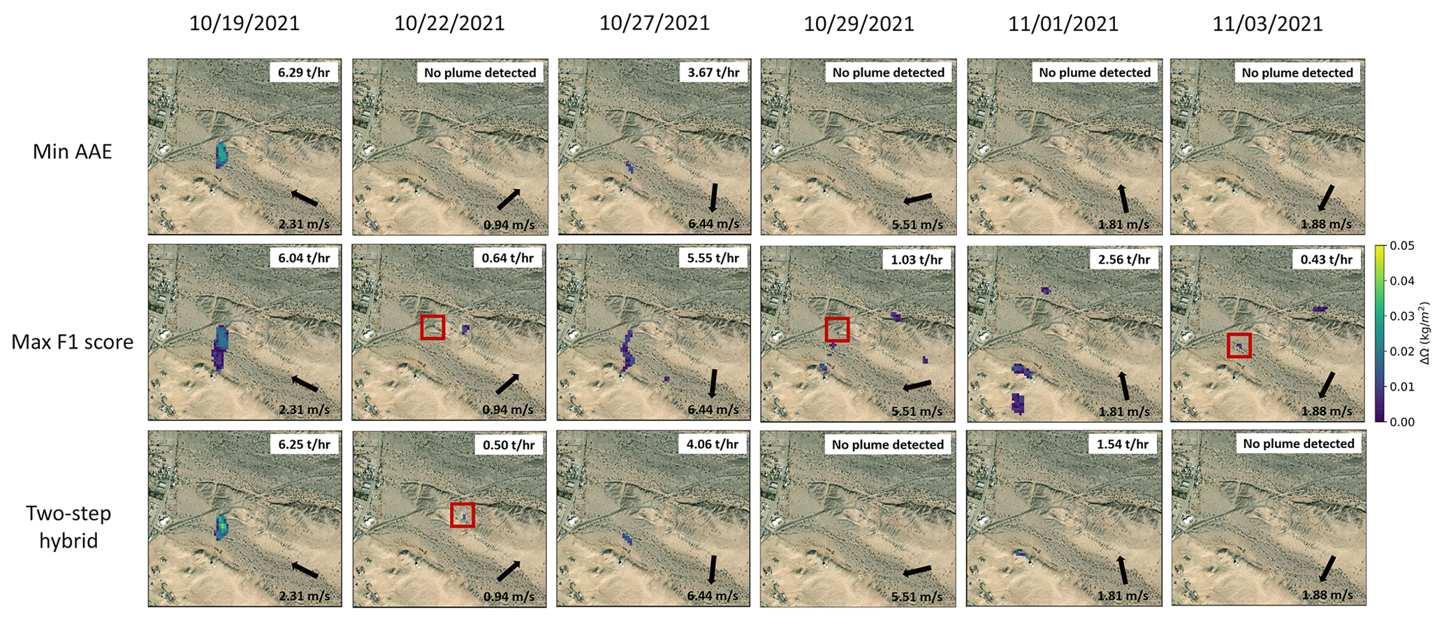
Figure 6Locations and shapes of the detected plumes. All the dates with plumes detected in “min AAE”, “max F1 score”, and “two-step hybrid” scenarios are shown. Plumes that are too small with only few pixels are marked in red, although they are not necessarily the full plume extent. Each figure also has the methane plume emission rate shown in the upper-right area and wind speed and direction shown in the lower-right area. Note that the plumes at 1 November 2021 are false positives since the ground-truth volume in this day is 0, and the dates with multiple plumes detected are also likely to include false positives, although this is hard to validate. The basemap is the ArcGIS Online World Imagery Basemap. The sources for the data used are as follows: Esri, DigitalGlobe, GeoEye, i-cubed, USDA FSA, USGS, AEX, Getmapping, Aerogrid, IGN, IGP, swisstopo, and the GIS User Community.
As a compromise, we developed a method to apply the MBPD algorithm in sequence to reduce the quantification error further while keeping a high F1 score. The specific steps are (1) apply a scenario with high F1 score as the base case to generate the first round of emission rate estimates, (2) raise the value of p and apply the updated scenario again to generate the second round of emission rate estimates, and (3) for the passes with non-zero emission rates in both scenarios, update the base case estimates to the new ones since they are likely to be closer to the ground-truth volumes. We name this method the “two-step application” method. Here we only change the value of p since the mask extraction step where p is applied is after the column retrieval step where bu and n are applied. So a consistent bu and n greatly reduce the computation workload as we only need to redo the mask extraction. Different from the direct application of the MBPD algorithm, this method is specifically designed to address the trade-off issue between quantification accuracy and detection accuracy. Table 1 shows an example of the two-step application (“two-step hybrid” scenario) with the “base case” scenario. Results show that the two-step hybrid scenario achieves lower AAE than the base case scenario with F1 score remaining the same. Specific locations and shapes of detected plumes in min AAE, max F1 score, and two-step hybrid scenarios are shown in Fig. 6.
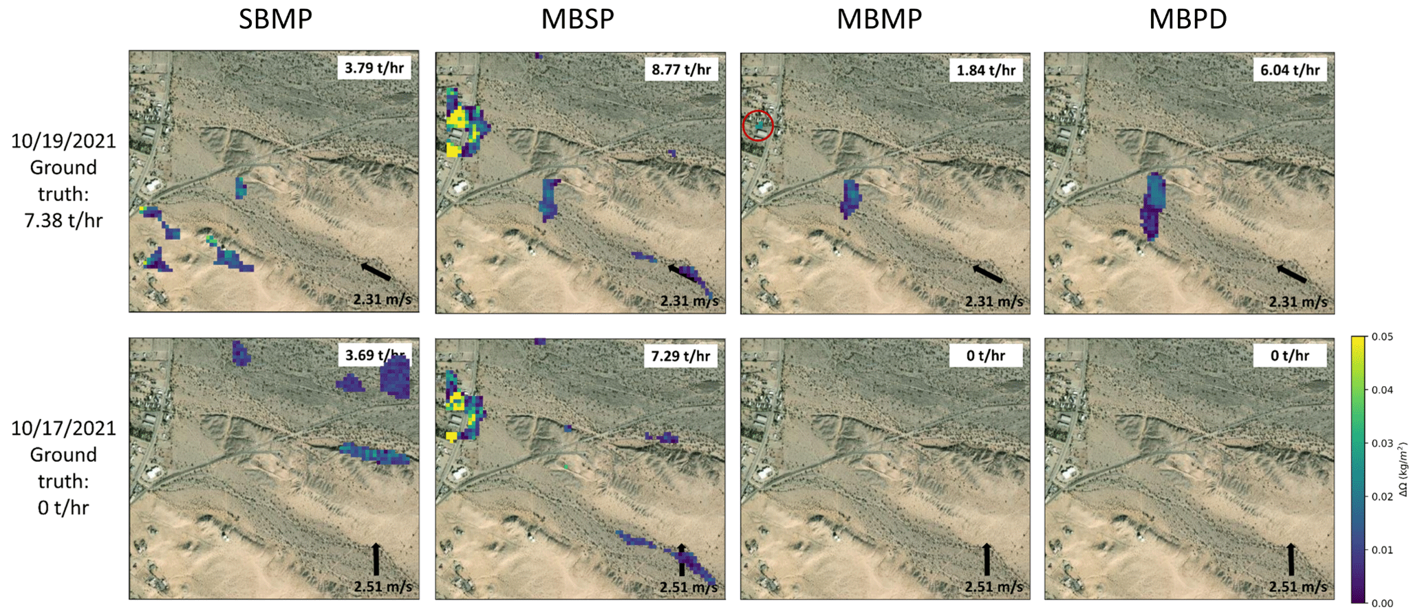
Figure 7Comparison of four retrieval methods. The performance of multi-band–multi-pass–multi-comparison-date (MBPD) algorithm is compared with multi-band–multi-pass (MBMP) method, multi-band–single-pass (MBSP) method and single-band–multi-pass (SBMP) method from Varon et al. (2021) for two dates, one with a methane plume (19 October 2021) and one with no plume (17 October 2021). The MBPD algorithm performs the best with correct yes/no detection and emission rate estimates closest to the ground-truth volumes. The MBMP retrieval has a small-area false positive detection on 19 October 2021 (red circle), and its emission rate estimate is much lower than the ground truth. MBSP and SBMP methods perform the worst with multiple large-area false positive plumes. The basemap is the ArcGIS Online World Imagery Basemap. The sources for the data used are as follows: Esri, DigitalGlobe, GeoEye, i-cubed, USDA FSA, USGS, AEX, Getmapping, Aerogrid, IGN, IGP, swisstopo, and the GIS User Community.
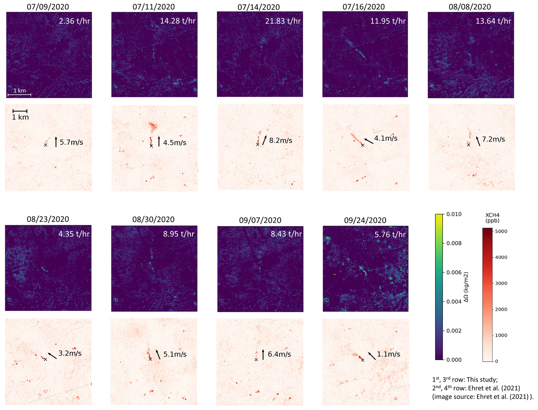
Figure 8Examination of true positives. The application site is in the Permian basin during the summer of 2020 studied in Ehret et al. (2022) (31.7335∘ N, 102.0421∘ W). The first and third rows show plume observation of this study, and the second and fourth rows show plume observation from Ehret et al. (2022) (image source: Ehret et al., 2022). All nine plumes represented in Ehret et al. (2022) were detected with similar shapes in this study. The emission rate estimate difference is within ±55 % of Ehret et al. (2022).
We also compared the performance of MBPD algorithm with the MBMP, MBSP, and SBMP methods from Varon et al. (2021) in Fig. 7. The top row is for a true emission rate of 7.38 t CH4 h−1, while the bottom row is for a true emission rate of 0 t CH4 h−1. Results show that the MBPD algorithm performs the best with both true positive and true negative detections. Its emission rate estimates are also the closest to the ground-truth volumes. The MBMP method has true negative detection in 17 October 2021 but shows a small false positive detection in 19 October 2021. Its emission rate estimate for this date is also much lower than the ground truth. This implies that the steps of normalization and inclusion of multiple comparison dates in the MBPD method contribute to a higher sensitivity to the true plume than the MBMP method. MBSP and SBMP retrievals perform worst with multiple large-area false positive plumes. The SBMP method is likely to produce false detections if the surface albedo changes across different passes, and the MBPD method reduces the effect of changing surface albedo by including different spectral bands and multiple comparison dates. The MBSP method can produce false detections because of the wavelength separation between two spectral bands, and the MBPD method largely removes these artifacts by subtracting the MBSP retrieval between different passes.
3.2 Broader application in cases of unknown emission rates
3.2.1 Examine true positives
To test the algorithm's performance in detecting true positives, we applied the algorithm in a methane-emitting site in the Permian basin during the summer of 2020 studied in Ehret et al. (2022). We used the parameters of the max F1 score scenario, which achieved the highest detection accuracy in the ground-truth calibration above. We detected all plumes from the 9 d covered in Ehret et al. (2022) with similar plume shapes and the emission rate estimate difference within ±55 %. This test validates the performance of detecting true positives of our method (Fig. 8).
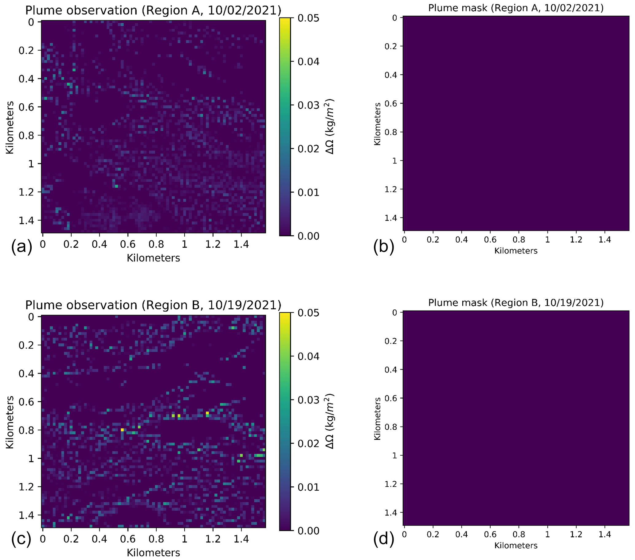
Figure 9Two examples of application studies. Panels (a) and (b) show an application case on 2 October 2021 in region A, and (c) and (d) show a case on 19 October 2021 in region B. Both examples have true negative detection. All of the other dates in the application studies have true negative detection as well.
3.2.2 Examine true negatives
To test the algorithm's performance in detecting true negatives, we applied the algorithm with the min AAE scenario since it achieved zero false positives in the ground-truth calibration above. Two application studies were designed, one in an extended 3-month time period from 1 October 2021 to 31 December 2021 in the same region as the controlled-release test (Fig. 4, region A) and one in a different region (Fig. 4, region B) in the same time period. The algorithm shows zero emissions in all the passes of both two studies, which validates its performance of detecting true negatives. Two detection examples are shown in Fig. 9.
This study presented a multi-band–multi-pass–multi-comparison-date (MBPD) methane retrieval algorithm using Sentinel-2 satellite imagery with several modifications based on the multi-band–multi-pass (MBMP) retrieval method from Varon et al. (2021). The major modification is including multiple comparison dates into the retrieval, which helps increase the contrast of the plume by stabilizing the background.
The new retrieval algorithm was then calibrated by a controlled-release test in Ehrenberg, Arizona in fall 2021. During calibration, three algorithm parameters were tuned based on the ground-truth emission rates to improve the algorithm performance. They are the pixel-level concentration upper-bound threshold bu for extreme value removal, the number of comparison dates n, and the pixel-level methane concentration percentage threshold p when determining the spatial extent of a plume. We found that although the algorithm sensitivity to bu is generally not very high, a low bu value can decrease its accuracy by resulting in false negatives. The n value should be high enough to enhance the algorithm sensitivity to the plumes in the target date, but values > 12 are neither necessary nor computationally efficient. A high p value helps enhance the quantification accuracy, but it may harm the yes/no detection accuracy by missing some true plumes.
The controlled-release calibration suggests that there is a trade-off between quantification accuracy and detection accuracy. If the algorithm aims to guarantee the quantification accuracy, then a bu in range 0.03–0.15, a n in range 7–14 and a p in range 0.91–0.92 are preferable. If the algorithm is expected to guarantee the detection accuracy, particularly with the fewest false negatives, then it would be more appropriate to choose bu at 0.02–0.12, n in the range 1–15, and p in the range 0.82–0.85. We also illustrate a two-step method that changes the parameter values and updates the emission rate estimates in an interim step, which improves quantification accuracy while keeping high yes/no detection accuracy.
To our knowledge, this is the first study that validates the performance of a Sentinel-2 methane detection and quantification algorithm by calibrating it with the ground-truth emission rates. We believe the ground-truth calibration offers researchers an opportunity to optimally tune methane retrieval algorithms and have confidence in their widespread deployment. In the future, the MBPD algorithm can be validated with more systematic experiments wherein the algorithm can be adjusted or tuned to meet different detection expectations.
We believe that the algorithm can still be improved further in the following aspects. First, the optimal values of three parameters may vary in different situations. For example, bu may vary with the methane plume volumes, n is affected by whether the plume is continuous or discrete in time, and p also depends on the area of the plume and the area of the study region, and thus it may vary with the study region size. In particular, this study is based on a homogeneous study area, and results may not generalize to heterogeneous sites with changing surface features during the study time period (e.g., due to seasonal shifts in vegetation). How to filter out outliers and define the true plume in a heterogeneous site is still difficult to answer since our controlled-release test covers only one region over a single month. In future controlled-release tests, we hope to explore these questions further based on more abundant ground-truth data in areas with more complex background features. Additionally, the current algorithm focuses more on removing false positives resulting from the background noise of the comparison dates. In real applications, however, more false positives due to the background noise of the target dates may be generated. Removing these false positives requires more work after the plume mask generation, such as removing the plume masks that are far away from well-known pad or pipeline locations. Other options may involve developing an automatic approach of outlier filtering and plume definition, as in Ehret et al. (2022), or applying machine vision based shape learning methods to filter out plume masks with shapes unlikely to be generated by a gas cloud. We hope to develop an efficient method of false detection removal so that Sentinel-2 can play a more important role in routine oil and gas methane monitoring in the global scale.
The methane detection and quantification algorithm code will be made available upon request. The methane column retrieval code will be made available for non-commercial use upon request (GHGSAT Data and Products – Copyright © 2021 GHGSAT Inc. All rights reserved). The Sentinel-2 satellite imagery are available in the Google Earth Engine (GEE) cloud platform, and the HRRR wind data are available in the AWS HRRR GRIB2 Archive. Both of the data collection codes will be made available upon request.
ZZ, EDS, DJV, and ARB contributed to the study conceptualization. ZZ conducted controlled-release calibration and application studies and wrote the manuscript with review and edits from all of the other authors.
The contact author has declared that none of the authors has any competing interests.
Publisher's note: Copernicus Publications remains neutral with regard to jurisdictional claims in published maps and institutional affiliations.
The authors acknowledge ExxonMobil and the Stanford Strategic Energy Alliance for funding the Ehrenberg controlled-release test.
This research has been supported by the California Air Resources Board (grant no. 18ISD011). The controlled-release test has been supported by ExxonMobil and the Stanford Strategic Energy Alliance.
This paper was edited by Joanna Joiner and reviewed by two anonymous referees.
Alvarez, R. A., Zavala-Araiza, D., Lyon, D. R., Allen, D. T., Barkley, Z. R., Brandt, A. R., Davis, K. J., Herndon, S. C., Jacob, D. J., Karion, A., Kort, E. A., Lamb, B. K., Lauvaux, T., Maasakkers, J. D., Marchese, A. J., Omara, M., Pacala, S. W., Peischl, J., Robinson, A. L., Shepson, P. B., Sweeney, C., Townsend-Small, A., Wofsy, S. C., and Hamburg, S. P.: Assessment of methane emissions from the US oil and gas supply chain, Science, 361, 186–188, https://doi.org/10.1126/science.aar7204, 2018.
Brandt, A. R., Heath, G. A., Kort, E. A., O'Sullivan, F., Pétron, G., Jordaan, S. M., Tans, P., Wilcox, J., Gopstein, A. M., Arent, D., Wofsy, S., Brown, N. J., Bradley, R., Stucky, G. D., Eardley, D., and Harriss, R.: Methane leaks from North American natural gas systems, Science, 343, 733–735, https://doi.org/10.1126/science.1247045, 2014.
Chen, Y., Sherwin, E. D., Berman, E. S., Jones, B. B., Gordon, M. P., Wetherley, E. B., Kort, E. A., and Brandt, A. R.: Quantifying Regional Methane Emissions in the New Mexico Permian Basin with a Comprehensive Aerial Survey, Environ. Sci. Technol., 56, 4317–4323, https://doi.org/10.1021/acs.est.1c06458, 2022.
Cusworth, D. H., Jacob, D. J., Varon, D. J., Chan Miller, C., Liu, X., Chance, K., Thorpe, A. K., Duren, R. M., Miller, C. E., Thompson, D. R., Frankenberg, C., Guanter, L., and Randles, C. A.: Potential of next-generation imaging spectrometers to detect and quantify methane point sources from space, Atmos. Meas. Tech., 12, 5655–5668, https://doi.org/10.5194/amt-12-5655-2019, 2019.
Cusworth, D. H., Duren, R. M., Thorpe, A. K., Olson-Duvall, W., Heckler, J., Chapman, J. W., Eastwood, M. L., Helmlinger, M. C., Green, R. O., Asner, G. P., Dennison, P. E., and Miller, C. E.: Intermittency of large methane emitters in the Permian Basin, Environ. Sci. Technol. Lett., 8, 567–573, https://doi.org/10.1021/acs.estlett.1c00173, 2021.
Ehret, T., De Truchis, A., Mazzolini, M., Morel, J.-M., D'aspremont, A., Lauvaux, T., Duren, R., Cusworth, D., and Facciolo, G.: Global tracking and quantification of oil and gas methane emissions from recurrent sentinel-2 imagery, Environ. Sci. Technol., 355 56, 10517–10529, https://doi.org/10.1021/acs.est.1c08575, 2022.
Frankenberg, C., Thorpe, A. K., Thompson, D. R., Hulley, G., Kort, E. A., Vance, N., Borchardt, J., Krings, T., Gerilowski, K., Sweeney, C., Conley, S., Bue, B. D., Aubrey, A. D., Hook, S., and Green, R. O.: Airborne methane remote measurements reveal heavy-tail flux distribution in Four Corners region, P. Natl. Acad. Sci. USA, 113, 9734–9739, https://doi.org/10.1073/pnas.1605617113, 2016.
Hausmann, P., Sussmann, R., and Smale, D.: Contribution of oil and natural gas production to renewed increase in atmospheric methane (2007–2014): top–down estimate from ethane and methane column observations, Atmos. Chem. Phys., 16, 3227–3244, https://doi.org/10.5194/acp-16-3227-2016, 2016.
Hu, H., Landgraf, J., Detmers, R., Borsdorff, T., Aan de Brugh, J., Aben, I., Butz, A., and Hasekamp, O.: Toward global mapping of methane with TROPOMI: First results and intersatellite comparison to GOSAT, Geophys. Res. Lett., 45, 3682–3689, https://doi.org/10.1002/2018GL077259, 2018.
IEA: Global Methane Tracker 2022, Tech. rep., IEA, https://www.iea.org/reports/global-methane-tracker-2022, last access: 6 July 2022.
Irakulis-Loitxate, I., Guanter, L., Maasakkers, J. D., Zavala-Araiza, D., and Aben, I.: Satellites Detect Abatable SuperEmissions in One of the World's Largest Methane Hotspot Regions, Environ. Sci. Technol., 56, 2143–2152, https://doi.org/10.1021/acs.est.1c04873, 2022.
Jacob, D. J., Turner, A. J., Maasakkers, J. D., Sheng, J., Sun, K., Liu, X., Chance, K., Aben, I., McKeever, J., and Frankenberg, C.: Satellite observations of atmospheric methane and their value for quantifying methane emissions, Atmos. Chem. Phys., 16, 14371–14396, https://doi.org/10.5194/acp-16-14371-2016, 2016.
Karion, A., Sweeney, C., Pétron, G., Frost, G., Michael Hardesty, R., Kofler, J., Miller, B. R., Newberger, T., Wolter, S., Banta, R., Brewer, A., Dlugokencky, E., Lang, P., Montzka, S. A., Schnell, R., Tans, P., Trainer, M., Zamora, R., and Conley, S.: Methane emissions estimate from airborne measurements over a western United States natural gas field, Geophys. Res. Lett., 40, 4393–4397, https://doi.org/10.1002/grl.50811, 2013.
Lauvaux, T., Giron, C., Mazzolini, M., d'Aspremont, A., Duren, R., Cusworth, D., Shindell, D., and Ciais, P.: Global assessment of oil and gas methane ultra-emitters, Science, 375, 557–561, https://doi.org/10.1126/science.abj4351, 2022.
MacKay, K., Lavoie, M., Bourlon, E., Atherton, E., O'Connell, E., Baillie, J., Fougère, C., and Risk, D.: Methane emissions from upstream oil and gas production in Canada are underestimated, Sci. Rep., 11, 1–8, https://doi.org/10.1038/s41598-021-87610-3, 2021.
Phiri, D., Simwanda, M., Salekin, S., Nyirenda, V. R., Murayama, Y., and Ranagalage, M.: Sentinel-2 data for land cover/use mapping: A review, Remote Sens., 12, 2291, https://doi.org/10.3390/rs12142291, 2020.
Rutherford, J. S., Sherwin, E. D., Ravikumar, A. P., Heath, G. A., Englander, J., Cooley, D., Lyon, D., Omara, M., Langfitt, Q., and Brandt, A. R.: Closing the methane gap in US oil and natural gas production emissions inventories, Nat. Commun., 12, 1–12, https://doi.org/10.1038/s41467-021-25017-4, 2021.
Rutherford, J. S., Sherwin, E. D., Chen, Y., and Brandt, A. R.: Controlled release experimental methods: 2021 Stanford controlled releases in TX and AZ, https://eao.stanford.edu/sites/g/files/sbiybj22256/files/media/file/Method_description_Setup_and_Uncertainty_v18.pdf, last access: 30 August 2022.
Sánchez-García, E., Gorroño, J., Irakulis-Loitxate, I., Varon, D. J., and Guanter, L.: Mapping methane plumes at very high spatial resolution with the WorldView-3 satellite, Atmos. Meas. Tech., 15, 1657–1674, https://doi.org/10.5194/amt-15-1657-2022, 2022.
Saunois, M., Stavert, A. R., Poulter, B., Bousquet, P., Canadell, J. G., Jackson, R. B., Raymond, P. A., Dlugokencky, E. J., Houweling, S., Patra, P. K., Ciais, P., Arora, V. K., Bastviken, D., Bergamaschi, P., Blake, D. R., Brailsford, G., Bruhwiler, L., Carlson, K. M., Carrol, M., Castaldi, S., Chandra, N., Crevoisier, C., Crill, P. M., Covey, K., Curry, C. L., Etiope, G., Frankenberg, C., Gedney, N., Hegglin, M. I., Höglund-Isaksson, L., Hugelius, G., Ishizawa, M., Ito, A., Janssens-Maenhout, G., Jensen, K. M., Joos, F., Kleinen, T., Krummel, P. B., Langenfelds, R. L., Laruelle, G. G., Liu, L., Machida, T., Maksyutov, S., McDonald, K. C., McNorton, J., Miller, P. A., Melton, J. R., Morino, I., Müller, J., Murguia-Flores, F., Naik, V., Niwa, Y., Noce, S., O'Doherty, S., Parker, R. J., Peng, C., Peng, S., Peters, G. P., Prigent, C., Prinn, R., Ramonet, M., Regnier, P., Riley, W. J., Rosentreter, J. A., Segers, A., Simpson, I. J., Shi, H., Smith, S. J., Steele, L. P., Thornton, B. F., Tian, H., Tohjima, Y., Tubiello, F. N., Tsuruta, A., Viovy, N., Voulgarakis, A., Weber, T. S., van Weele, M., van der Werf, G. R., Weiss, R. F., Worthy, D., Wunch, D., Yin, Y., Yoshida, Y., Zhang, W., Zhang, Z., Zhao, Y., Zheng, B., Zhu, Q., Zhu, Q., and Zhuang, Q.: The Global Methane Budget 2000–2017, Earth Syst. Sci. Data, 12, 1561–1623, https://doi.org/10.5194/essd-12-1561-2020, 2020.
Sherwin, E. D., Chen, Y., Ravikumar, A. P., and Brandt, A. R.: Single-blind test of airplane-based hyperspectral methane detection via controlled releases, Elem. Sci. Anth., 9, 00063, https://doi.org/10.1525/elementa.2021.00063, 2021.
Thompson, D., Thorpe, A., Frankenberg, C., Green, R., Duren, R., Guanter, L., Hollstein, A., Middleton, E., Ong, L., and Ungar, S.: Space-based remote imaging spectroscopy of the Aliso Canyon CH4 superemitter, Geophys. Res. Lett., 43, 6571–6578, https://doi.org/10.1002/2016GL069079, 2016.
US NOAA: The High-Resolution Rapid Refresh (HRRR), U.S. NOAA [data set], https://rapidrefresh.noaa.gov/hrrr/ (last access: 15 March 2022), 2021.
Varon, D. J., Jacob, D. J., McKeever, J., Jervis, D., Durak, B. O. A., Xia, Y., and Huang, Y.: Quantifying methane point sources from fine-scale satellite observations of atmospheric methane plumes, Atmos. Meas. Tech., 11, 5673–5686, https://doi.org/10.5194/amt-11-5673-2018, 2018.
Varon, D. J., Jacob, D. J., Jervis, D., and McKeever, J.: Quantifying time-averaged methane emissions from individual coal mine vents with GHGSat-D satellite observations, Environ. Sci. Technol., 54, 10246–10253, https://doi.org/10.1021/acs.est.0c01213, 2020.
Varon, D. J., Jervis, D., McKeever, J., Spence, I., Gains, D., and Jacob, D. J.: High-frequency monitoring of anomalous methane point sources with multispectral Sentinel-2 satellite observations, Atmos. Meas. Tech., 14, 2771–2785, https://doi.org/10.5194/amt-14-2771-2021, 2021.
Veefkind, J., Aben, I., McMullan, K., Förster, H., de Vries, J., Otter, G., Claas, J., Eskes, H., de Haan, J., Kleipool, Q., van Weele, M., Hasekamp, O., Hoogeveen, R., Landgraf, J., Snel, R., Tol, P., Ingmann, P., Voors, R., Kruizinga, B., Vink, R., Visser, H., and Levelt, P.: TROPOMI on the ESA Sentinel-5 Precursor: A GMES mission for global observations of the atmospheric composition for climate, air quality and ozone layer applications, Remote Sens. Environ., 120, 70–83, https://doi.org/10.1016/j.rse.2011.09.027, 2012.
Zavala-Araiza, D., Lyon, D. R., Alvarez, R. A., Davis, K. J., Harriss, R., Herndon, S. C., Karion, A., Kort, E. A., Lamb, B. K., Lan, X., Marchese, A. J., Pacala, S. W., Robinson, A. L., Shepson, P. B., Sweeney, C., Talbot, R., Townsend-Small, A., Yacovitch, T. I., Zimmerle, D. J., and Hamburg, S. P.: Reconciling divergent estimates of oil and gas methane emissions, P. Natl. Acad. Sci. USA, 112, 15597–15602, https://doi.org/10.1073/pnas.1522126112, 2015.