the Creative Commons Attribution 4.0 License.
the Creative Commons Attribution 4.0 License.
 | 14 Feb 2022
Applying self-supervised learning for semantic cloud segmentation of all-sky images
Bijan Nouri
Stefan Wilbert
Niklas Blum
Rudolph Triebel
Marcel Hasenbalg
Pascal Kuhn
Luis F. Zarzalejo
Robert Pitz-Paal
Semantic segmentation of ground-based all-sky images (ASIs) can provide high-resolution cloud coverage information of distinct cloud types, applicable for meteorology-, climatology- and solar-energy-related applications. Since the shape and appearance of clouds is variable, and there is high similarity between cloud types, a clear classification is difficult. Therefore, most state-of-the-art methods focus on the distinction between cloudy and cloud-free pixels without taking into account the cloud type. On the other hand, cloud classification is typically determined separately at the image level, neglecting the cloud's position and only considering the prevailing cloud type. Deep neural networks have proven to be very effective and robust for segmentation tasks; however they require large training datasets to learn complex visual features. In this work, we present a self-supervised learning approach to exploit many more data than in purely supervised training and thus increase the model's performance. In the first step, we use about 300 000 ASIs in two different pretext tasks for pretraining. One of them pursues an image reconstruction approach. The other one is based on the DeepCluster model, an iterative procedure of clustering and classifying the neural network output. In the second step, our model is fine-tuned on a small labeled dataset of 770 ASIs, of which 616 are used for training and 154 for validation. For each of them, a ground truth mask was created that classifies each pixel into clear sky or a low-layer, mid-layer or high-layer cloud. To analyze the effectiveness of self-supervised pretraining, we compare our approach to randomly initialized and pretrained ImageNet weights using the same training and validation sets. Achieving 85.8 % pixel accuracy on average, our best self-supervised model outperforms the conventional approaches of random (78.3 %) and pretrained ImageNet initialization (82.1 %). The benefits become even more evident when regarding precision, recall and intersection over union (IoU) of the respective cloud classes, where the improvement is between 5 and 20 percentage points. Furthermore, we compare the performance of our best model with regards to binary segmentation with a clear-sky library (CSL) from the literature. Our model outperforms the CSL by over 7 percentage points, reaching a pixel accuracy of 95 %.
- Article
(2273 KB) - Full-text XML
- BibTeX
- EndNote


Clouds constantly cover large fractions of the globe, influencing the amount of shortwave radiation reflected, transmitted and absorbed by the atmosphere. Therefore, they not only affect momentarily local temperatures but also play a significant role in climate change (Rossow and Zhang, 1995; Rossow and Schiffer, 1999; Stubenrauch et al., 2013). The actual impact on solar irradiation depends on the properties of individual clouds and is still a current field of research. Automatic detection and specification of clouds can thus help to study their effects in more detail and to monitor changes that may be induced by climate change. Moreover, cloud data is essential for weather forecasts and solar energy applications. In so-called nowcasting systems for example, shortwave solar irradiation is forecasted in intra-minute and intra-hour time frames using ground-based observations. These forecasts have proven to be beneficial for the operation of solar power plants (Kuhn et al., 2018) and have the potential to optimize power distribution of solar energy over electricity nets (Perez et al., 2016).
Ground-based measurements and satellite measurements are the two possibilities for continuously observing clouds. While satellite images cover larger areas, they are also less detailed. On the other hand, ground-based sky observations using all-sky imagers have limited coverage, but they can be obtained in higher temporal and spatial resolution. Therefore, all-sky imagers represent a valuable complement to satellite imaging that is being studied increasingly. In the past various ground-based camera systems were developed for automatic cloud cover observations (Shields et al., 1998; Long et al., 2001; Widener and Long, 2004). Furthermore, off-the-shelf surveillance cameras are frequently utilized (West et al., 2014; Blanc et al., 2017; Nouri et al., 2019b). They all observe the entire hemisphere using fish-eye lenses with a viewing angle of about 180∘. Thereby, typical cloud heights and clouds spread over multiple square kilometers can be monitored. In this work we refer to these cameras as all-sky imagers and the corresponding images as ASIs.
Usually, there are two tasks most studies distinguish between. In cloud detection, the precise location of a cloud within the ASI is sought, whereas cloud specification aims to provide information about the properties of an observed cloud. The former is achieved by segmenting the image into cloudy and cloudless pixels. For the latter, the common approach is to classify visible clouds into specified categories of cloud types. Often, classification is based on the 10 main cloud genera defined by the World Meteorological Organization (WMO) (Cohn, 2017). Both tasks are challenging for a number of reasons. For instance, a clear distinction between aerosols and clouds is not always possible from image data. Corresponding to Calbó et al. (2017), clouds are defined by the visible number of water droplets and ice crystals. In contrast, aerosols comprise all liquid and solid particles independent of their visibility. Still, the underlying phenomenon is the same, and there is no clear demarcation between one and the other. Moreover, cloud fragments can extend multiple kilometers into their surroundings, mixing with other aerosols in a so-called twilight zone (Koren et al., 2007). This absence of sharp boundaries makes precise segmentation particularly difficult. For classification, high similarities between cloud types and large variations in spatial extent pose another challenge. Furthermore, the appearances of clouds are influenced by atmospheric conditions, illuminations and distortion effects from the fish-eye lenses. Finally, overlapping cloud layers are especially difficult to distinguish. As a result, many datasets intentionally neglect such multi-layer conditions or consider the prevailing cloud type only.
Traditionally, segmentation and classification were addressed separately. Firstly, both tasks are hard to solve individually. Secondly, the solution approaches are often very distinct. Most segmentation techniques rely on threshold-based methods in color space. One commonly applied measure is the red–blue ratio (Long et al., 2006) or difference (Heinle et al., 2010) within the RGB color space. Other methods include the green channel as well (Kazantzidis et al., 2012), apply adaptive thresholding (Li et al., 2011) or transform the image into HSI (hue–saturation–intensity) color space (Souza-Echer et al., 2006; Jayadevan et al., 2015). Also super-pixel segmentation, graph models and combination of both have already been studied for threshold-based cloud segmentation (Liu et al., 2014, 2015; Shi et al., 2017). The problem with thresholds is that they depend on many factors, such as sun elevation, a pixel's relative position to the sun or horizon, and current atmospheric conditions. To take these factors into account, clear-sky libraries (CSLs) were introduced (Chow et al., 2011; Ghonima et al., 2012; Chauvin et al., 2015; Wilbert et al., 2016; Kuhn et al., 2018). CSLs store historical RGB data from clear-sky conditions, which are used to compute a reference image of the threshold color feature (e.g., red–blue ratio). By considering the difference image from reference and original color features, detection is more robust.
Apart from manually adjusting thresholds of color features, learning-based methods were examined, too. To identify the most relevant color components, clustering and dimensionality reduction techniques were applied (Dev et al., 2014, 2016). There are also studies on supervised learning techniques for classifying pixels in ASIs such as neural networks, support vector machines (SVMs), random forests and Bayesian classifiers (Taravat et al., 2014; Cheng and Lin, 2017; Ye et al., 2019). Lately, also deep learning approaches using convolutional neural networks (CNNs) were presented (Dev et al., 2019; Xie et al., 2020; Song et al., 2020). Although, they were trained in a purely supervised manner using relatively small datasets, the results outperform threshold-based state-of-the-art methods significantly. This corresponds to a recent benchmark on cloud segmentation methods (Hasenbalg et al., 2020). Different threshold-based methods and a CNN were evaluated in a diverse dataset of 829 manually segmented ASIs. In this comparison the CNN performed best.
However, most techniques presented in the literature still focus on binary segmentation and do not differentiate between cloud types. Until today, cloud classification has been mainly studied at the image level, independent of the segmentation approach. Therefore, many datasets contain cutouts of ASIs (“sky patches”). Others are based on camera images with a smaller field of view, or ambiguous ASIs were omitted entirely.
For classification, most approaches are learning-based. Various classifiers, like k nearest neighbors, support vector machines and CNNs, have been trained to recognize the depicted cloud type (Heinle et al., 2010; Zhuo et al., 2014; Ye et al., 2017; Zhang et al., 2018). The classes are usually based on the main cloud genera, sometimes combining visually similar types.
Recently, the combination of both tasks, leading to semantic segmentation, has been targeted as well. In two studies, clouds were distinguished in thin and thick clouds (Dev et al., 2015, 2019), however only considering a small dataset of 32 images of sky patches. To our knowledge, there is only one work of an extensive segmentation approach, which is based on 9 cloud genera using 600 labeled ASIs (Ye et al., 2019). The authors propose to extract and transform a set of features for generated super-pixels and classify each of them using an SVM. They evaluate their method by comparing the results with a CNN that could not achieve the same accuracy. The problem with deep learning in this case is the lack of data to learn relevant features and complex data correlations to distinguish between cloud types. Therefore, we propose self-supervised pretraining to enable the model to better learn complex features.
Self-supervised learning is a form of unsupervised learning that does not require manually created labels but generates pseudolabels from the data themselves. A model is trained by solving a pretext task, a pre-designed task for learning data representations. Afterwards, representation learning is evaluated in a downstream task. Usually this is done by applying transfer learning, thus using pretrained weights as initialization, and fine-tuning a model using a small labeled dataset. In the field of natural language processing, it has become common practice to pretrain a so-called language model, for instance by predicting the following word in a text (Howard and Ruder, 2018). Lately also in computer vision a trend of self-supervised learning can be observed (Radford et al., 2015; Doersch et al., 2015; Pathak et al., 2016; Noroozi and Favaro, 2016; Lee et al., 2017; Caron et al., 2018).
In this work we apply two different pretext tasks for self-supervised learning. The first comprises two sub-tasks to be solved. One is to fill cropped areas (Pathak et al., 2016), and the other is to increase the image resolution (Johnson et al., 2016). We refer to it as the inpainting and super-resolution (IP–SR) method. Secondly, we apply the winner of a benchmark on self-supervised learning for computer vision (Jing and Tian, 2020), which is called DeepCluster (Caron et al., 2018). It is based on an iterative process of clustering the feature outputs from a deep net and using the cluster assignments as pseudolabels for classification.
By applying self-supervised learning, the limits of a purely supervised approach involving time-consuming and manual creation of ground truth segmentation masks can be overcome. Consequently, the models can be trained with many more data, learning more general and complex features to distinguish cloud types. To our knowledge, this work presents the first approach of applying deep learning for semantic cloud segmentation on unlabeled data and a new classification of clouds into three layers. The remainder of this work is organized as follows: in Sect. 2, the datasets for supervised fine-tuning and self-supervised pretraining are presented. Section 3 introduces the model architecture and the chosen hyperparameters for training. In Sect. 4, the trained models are evaluated. First, the results of the pretext tasks are analyzed. Afterwards, the performance of semantic segmentation using self-supervision is compared to a randomly initialized model and another one pretrained using ImageNet. Then the results of binary segmentation are compared to the results of a CSL in the same dataset. Finally, we conclude our work and provide a brief outlook in Sect. 5.
In this section, the data used for training are described. First, some details about hardware and image properties are given. Then the image selection for the labeled and the unlabeled datasets is discussed.
2.1 Image acquisition
All images for training and validating our models were taken at CIEMAT's1 Plataforma Solar de Almeria (PSA). It is located in the desert of Tabernas (Spain), where atmospheric conditions are often clear, but the observed cloud formations are versatile and multi-layered. For our datasets we used a single all-sky imager based on an off-the-shelf surveillance camera from Mobotix (model Q25). Images are captured and stored with a resolution of 4.35 MP. However, they are cropped and resized to a square format of 512×512 pixels for the input of the network. Moreover, the images are preprocessed by overlaying a camera mask that removes static objects from the site surroundings. Exposure time is fixed at 160 µs, and no solar occulting devices are installed. The camera is set to take a picture every 30 s from sunrise to sunset, resulting in approximately 1000 to 1600 images per day.
2.2 Labeled dataset
For differentiating between cloud types, we categorize clouds into three classes: low-, middle- and high-layer clouds. They combine the 10 main genera defined by the WMO (Cohn, 2017) depending on typical cloud base heights. While low-layer clouds are usually dense and heavy clouds of liquid water, high-layer clouds are generally thinner and contain ice particles only. Mid-layer clouds occur in between and contain a varying quantity of water and ice particles. Consequently, also the optical characteristics of clouds within these layers are different. Another reason for classifying clouds into three layers is to detect multi-layer conditions. Particularly for solar irradiation forecasting, it is important to determine cloud dynamics, which often vary in direction and propagation speed for clouds of different layers.
Our labeled dataset is based on a selection from Hasenbalg et al. (2020). As the original ground truth segmentation masks used in Hasenbalg et al. (2020) are only binary, we revised 669 images and segmented 101 new images from the same camera, all captured in 2017. In particular images containing thin high-layer clouds and difficult multi-layer conditions were added, such that a more balanced distribution of cloud types was attained. Furthermore, the selection covers a large variety of sun elevations and Linke turbidity (TL), representing diverse atmospheric conditions. The Linke turbidity coefficient describes the extinction of the solar irradiance as a multiplier of clean and dry ideal atmospheres, and it can be derived from the direct normal irradiation (DNI) according to Ineichen and Perez (2002). In Fig. 1 an overview of the dataset is given.

Figure 1Distribution of labeled dataset with respect to cloud types, sun elevation (α) and Linke turbidity (TL). For cloud layers (leftmost plot), the labels describe the total number of ASIs containing respective layers or combinations. For instance, an ASI with low- and high-layer clouds counts for low-layer, high-layer, and low-layer and high-layer.
2.3 Unlabeled dataset for self-supervised pretraining
The unlabeled dataset includes ASIs from the whole year 2017 covering a large variety of conditions. To reduce computation effort, the dataset was filtered, neglecting images that do not contribute much to the learning process. In particular, images with clear-sky conditions are not very useful. Therefore, approximately 40 % of all images were sorted out using reference DNI measurements and a classification procedure as described in Nouri et al. (2019a). As a result, this dataset comprises 286 477 ASIs.
In this section details about the model architectures and hyperparameters for supervised segmentation and pretraining are provided.
3.1 Details of the segmentation model
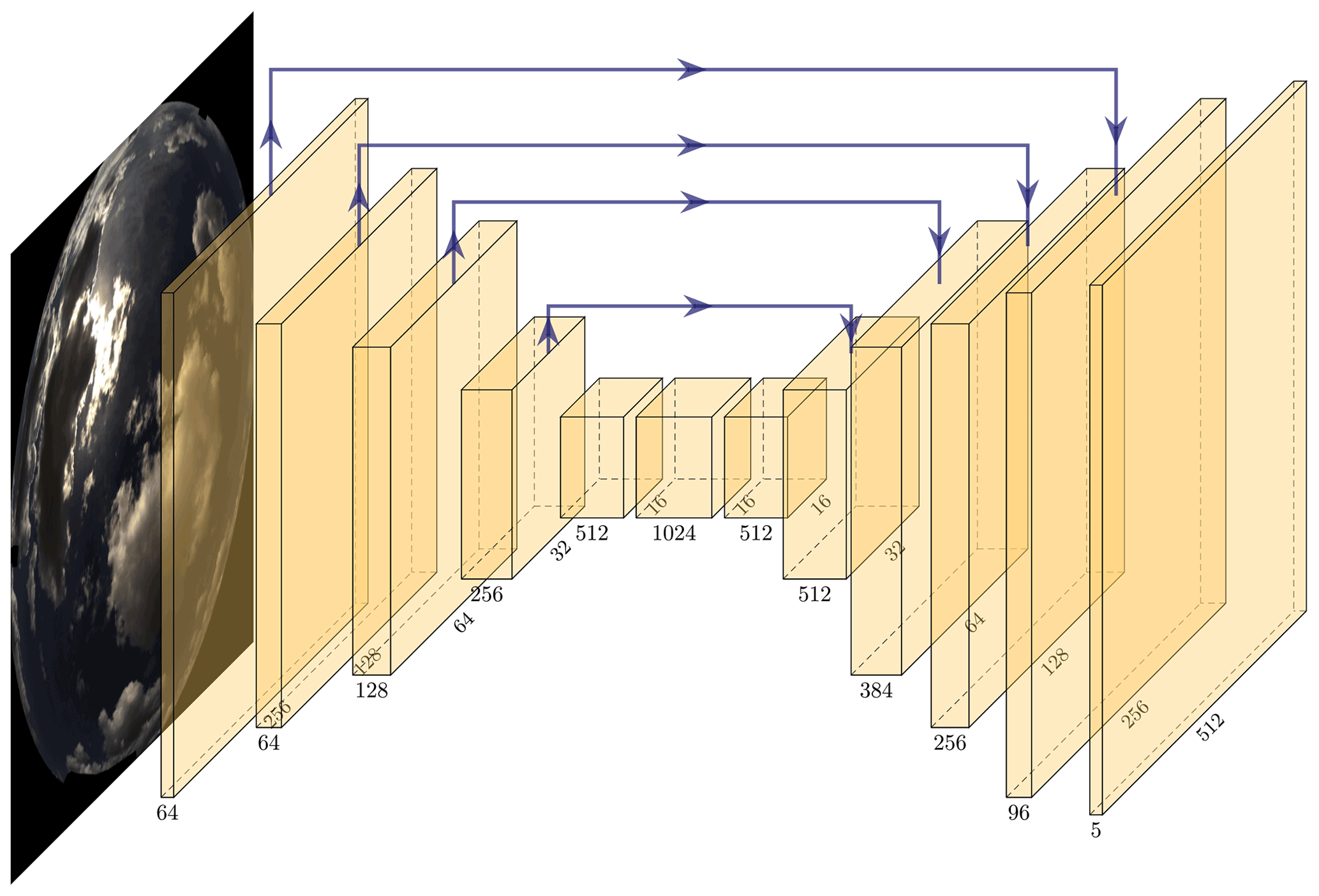
The architecture of our deep learning model is based on a U-Net (Ronneberger et al., 2015). A U-Net is a fully convolutional network (Shelhamer et al., 2017) which is composed of an encoder and a decoder part. The encoder part represents the usual downsampling path and consists of a standard ResNet34 (He et al., 2016) in our case. The decoder uses deconvolutions to upsample the resulting dense representations to the original input size. The special feature of U-Nets is the symmetrical, U-shaped structure of the encoder and decoder with skip connections in between. These connections concatenate the output of a directly preceding layer with the batch-normalized output (Ioffe and Szegedy, 2015) of the respective encoder layer. Hence, feature channels in the decoder contain context information which is propagated to higher resolutions, enabling precise localization of features. The expansion of the input feature map itself, thus creating new pixels in between, is achieved by applying the so-called pixel-shuffle method (Shi et al., 2016; Aitken et al., 2017). Overall, our decoder consists of multiple blocks performing input expansion and merging and applying convolutions and non-linear activations (see Fig. 2). In total there are four of these blocks and a final output layer producing an output tensor of . The fifth dimension in this tensor is required for the black outer area of the image produced by the fish-eye-lens cameras. The cloud class (y) is then predicted for each pixel (z) by applying the softmax function (σ) over the five channels (C=5) and computing the arg max (index of maximum in respective vector):
An overview of the entire architecture is shown in Fig. 3.
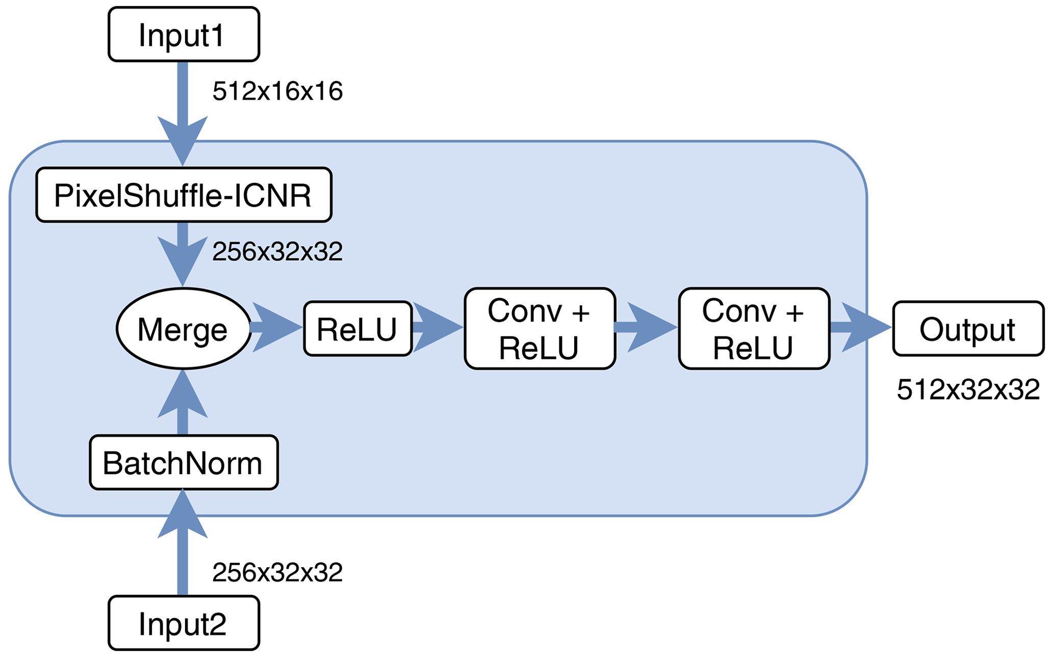
Figure 2Diagram of exemplary inner deconvolution block. Input1 refers to the output from the preceding layer, whereas Input2 indicates a skip connection from the corresponding layer in the encoder part. After merging, convolutions and non-linear activations (ReLU) are applied to produce the upsampled output of this block.
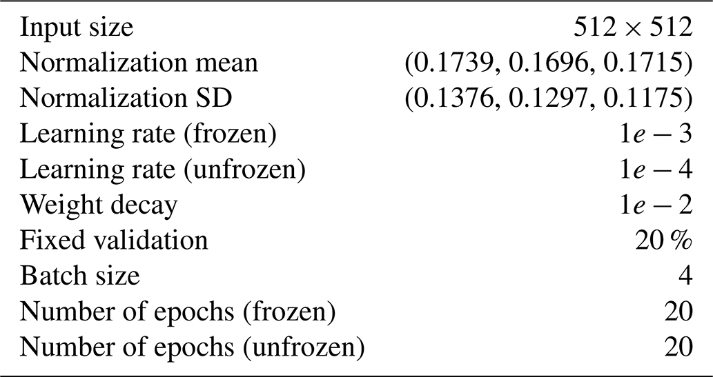
For data augmentations we apply 90∘ rotations and horizontal and vertical flips with a probability of 75 % for each batch. In the case of the self-supervised models, the input is normalized color-channel-wise by subtracting the mean and dividing by the standard deviation of the unlabeled dataset. We use standard cross-entropy as loss function and the Adam optimizer (Kingma and Ba, 2014) with default parameters. Weights of non-pretrained network parts are initialized with Kaiming initialization (He et al., 2015), and we apply weight decay to prevent overfitting. Furthermore, we apply a learning rate finder and one-cycle policy as described in Smith (2017, 2018). To obtain faster convergence, we split training into two phases. In the first phase, the pretrained encoder part is frozen for 20 epochs using a larger learning rate. Afterwards, the entire network is fine-tuned with a smaller one for another 20 epochs. These values were chosen after examining the loss curves for the training and validation set for longer training runs. The network is trained in batches of 4 images using 80 % of the dataset, which leaves 154 images for validation. All models are trained using a single graphics processing unit (GPU), a Nvidia GeForce RTX 2080 Super, and were implemented using fastai v1 (Howard et al., 2018), a high-level PyTorch (Paszke et al., 2019) API. A summary of the hyperparameter selection is given in Table 1.
3.2 Pretext tasks for self-supervised learning
As mentioned before, we implemented two methods for self-supervised learning based on techniques which have proven to be successful in the literature: IP–SR and DeepCluster (DC).
For the IP–SR task, the original image is corrupted by inserting four black squares and by reducing the resolution by half. The square boxes are positioned randomly within the ASI and have an edge length of 80 pixels. This size was chosen such that smaller clouds can be occluded, but general cloudiness conditions can still be determined by human observers. Furthermore, after downsizing the images they need to be upscaled again to match the network's input size, which is achieved using bilinear interpolation. For inpainting, the model should learn to predict the missing parts by observing and recognizing the surrounding conditions. Regarding super-resolution, the model should learn structural and textural characteristics of clouds, which helps to better distinguish cloud types in later segmentation. For this task, the architecture is the same as for the segmentation model (apart from the output layer), and also the hyperparameters are mostly equal. The loss is composed of a pixel-wise MAE and a so-called perceptual loss (Johnson et al., 2016). Due to limited GPU memory and high computational efforts, batch size was limited to 2, and training consists of 10 epochs.
The DeepCluster method (Caron et al., 2018) follows the approach of creating pseudolabels that can be used for classification. Thereby, the network should learn useful data representations that are relevant to recognize objects, or in our case clouds. It consists of two alternating steps. (1) The output features of the CNN (ResNet34 encoder part) are assigned to a predefined number of clusters. For this we apply a standard k-means algorithm. (2) The resulting cluster assignments can then be used as pseudolabels to solve a standard classification problem. After each epoch (clustering + classification), the features are clustered again, leading to new pseudolabels. According to Caron et al. (2018), k should be set higher than the target classes. Hence, to choose a reasonable value for k, we evaluated three models using . Hyperparameters were mostly adopted from the original DeepCluster setup; only batch size and the number of epochs were set to 32 and 50, respectively.
For both pretext tasks (IP–SR and DC), we tested two weight initializations: first, standard random (Kaiming) initialization (i.e., the network starts with random weights), and secondly, initialization with pretrained ImageNet weights. Hence, the ResNet34 part is initialized with weights of a ResNet34 model that was trained using ImageNet. These are available online and can be downloaded via PyTorch.
Next, we briefly examine the models from self-supervised pretraining. However, the major part deals with the segmentation results of the validation set of our labeled data.
4.1 Pretraining results
The pretraining results are only evaluated qualitatively to check whether our models learned to solve the tasks sensibly. Regarding IP–SR, Fig. 4 shows an example of an ASI section of the input, the prediction and the ground truth (original) image. Here, it can be seen that the part of the black box is indeed filled similarly to the cirrus clouds which were occluded. Even small parts of the neighboring altocumulus clouds in the upper right corner are reconstructed. Also, more structural and textural details are present in the predicted image compared to the input. However, there are also some artifacts visible in the reconstructed area, and there is still a notable difference to the original resolution. We chose this particular image section as the occluded part contains two cloud layers, and it can be seen that the model's predictions for the black box depend on the surrounding conditions. Clearly, this exemplary instance does not prove the general capability of the model to make reasonable predictions for the entire dataset. However, as we could not find any unexpected pixel reconstructions on multiple days of generated ASIs under various conditions, a successful learning effect can be assumed.
In the case of DeepCluster, we examined exemplary samples that were classified based on the final cluster assignments. Figure 5 depicts four randomly picked ASIs of four different clusters. In this example, the model was trained with k=30 clusters. It can be observed that the clusters consider general cloudiness conditions like cloud coverage but also focus on sun elevation and turbidity. In the upper row, even raindrops on the lenses seem to be a characteristic feature for this cluster assignment.
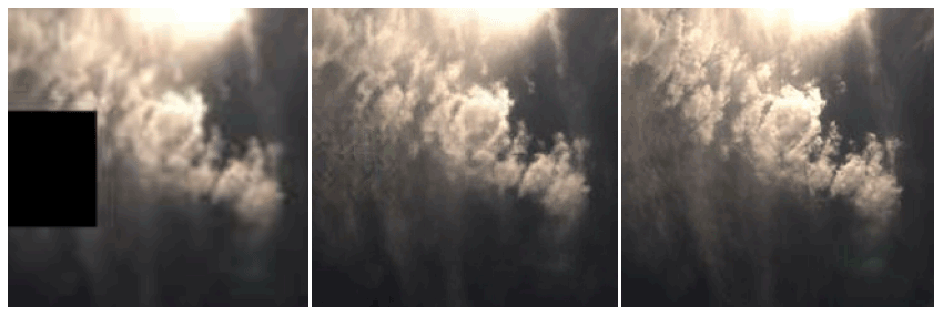
Figure 4From left to right: input, prediction and ground truth in inpainting–super-resolution pretext task.
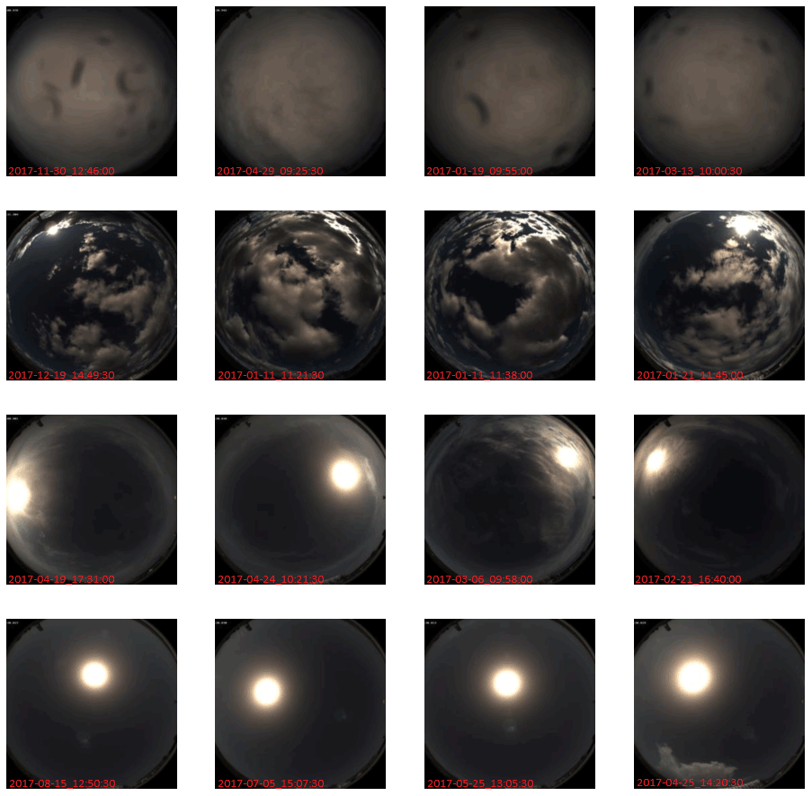
Figure 5Four randomly chosen samples of four clusters after training. The images of each row correspond to one cluster.
4.2 Segmentation results
To evaluate overall segmentation performance, we use two commonly applied metrics: first, pixel accuracy, which is defined by the number of correctly predicted ASI pixels divided by the number of all ASI pixels (NumPix), and secondly, mean intersection over union (IoU), the overlapping area of predicted and target pixels by their union. The border part of the ASI, indicating masked image areas (see Sect. 2.2), is neglected as this would distort the results. Furthermore, we also evaluate precision, recall and IoU for each class to analyze segmentation in more detail. These metrics are normalized corresponding to the number of (predicted and target) pixels of the respective class. Thus, the size of an observed cloud type is considered for computing the metrics' averages. Our evaluation metrics are therefore defined as
where TP and FP (TN and FN) refer to true and false positives (true and false negatives), respectively; the index c to one of the cloud classes; and N to the number of ASIs.
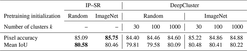
First we compared different training setups of the pretext tasks. Apart from pretraining initialization, this comprises also the different values for k in the DeepCluster pretraining. After pretraining, the trained weights of the ResNet34 part are transferred to the segmentation model, fine-tuned using the training set and evaluated for the validation set. Table 2 summarizes the results for pixel accuracy and mean IoU. In all setups the differences are rather small. Pixel accuracy is between 84.6 % and 85.8 %, whereas mean IoU is always slightly over 80 %. Hence, no significant improvement using ImageNet initialization for self-supervised pretraining can be observed. The influence of k on the segmentation task is also small, but smaller values seem to lead to marginally better results.
Table 2Comparison of segmentation results when testing different training setups for self-supervised pretraining. Best values are highlighted in bold.
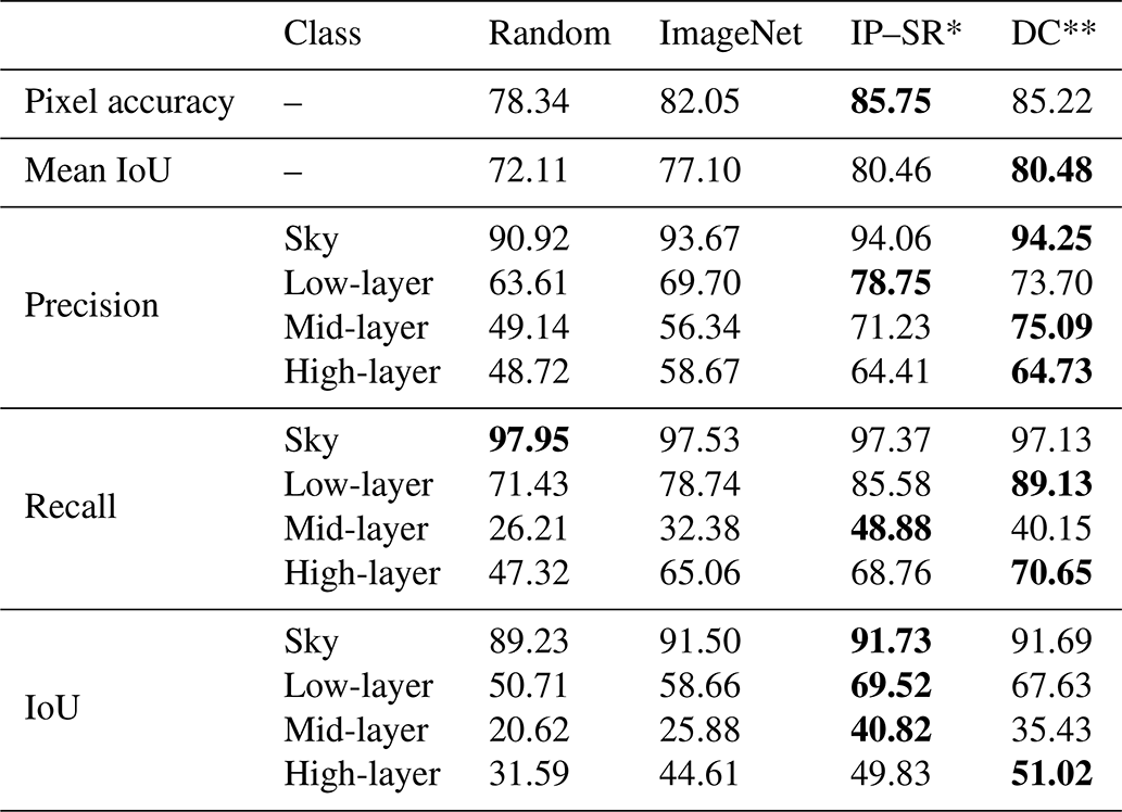
In the next step, we compare our self-supervised approach to standard supervised training with random and ImageNet initialization. All the following statements are based on Table 3. For a better overview, only the best self-supervised models in terms of pixel accuracy are considered here (DC and IP–SR with ImageNet initialization and DC with k=30). Regarding overall pixel accuracy and mean IoU, our self-supervised approaches reach over 3 percentage points more than starting with ImageNet and about 7 percentage points more than with random initialization. Concerning the prediction of cloud classes, a more significant improvement becomes evident. On average, precision, recall and IoU are about 9–10 percentage points higher for the self-supervised IP–SR approach compared to ImageNet initialization. For the mid-layer class, it is about 15 percentage points. Also our DC method outperforms the purely supervised approaches significantly, reaching similar values on average as the IP–SR method. Overall, self-supervised learning achieves the best results except for recall of sky. However, this is negligible as all approaches reach values over 97 %, and corresponding precision is significantly lower, indicating overestimation.
Table 3Segmentation results comparing our self-supervised approaches with standard ImageNet or random initialization. IP–SR* and DC** refer to pretraining starting with ImageNet weights and k=30 for the DC method. Best values are highlighted in bold.
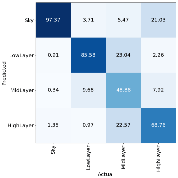
To further interpret segmentation results, we analyze misclassification using a confusion matrix shown in Fig. 6. Most frequent confusions are between adjacent cloud layers, which is why the mid-layer class is predicted to be the worst. Also high-layer clouds are sometimes not detected at all. On the other hand, low- and high-layer clouds can be distinguished quite reliably.
When examining exemplary segmentation masks as depicted in Fig. 7, another problem becomes apparent. Thinner parts of low-layer clouds are sometimes misclassified as mid- or even high-layer clouds since they typically occur in twilight zones. Moreover, the decrease in classification accuracy for lower elevation angles is expected because the fish-eye lenses capture these areas with lower resolution. Another challenge is stratus-like overcasts. These clouds often lack texture; they can have variable depth, and they can occur in all layers, which makes it particularly hard to differentiate. A very challenging cloud condition is shown in the lower example of Fig. 7, which combines a lot of the challenges just mentioned. Although it recognizes parts of the low-layer clouds, the model seems to be uncertain about the specific cloud layers as it often changes between all three classes. Nevertheless, the accuracy regarding cloudy and cloud-free pixels is still very high.
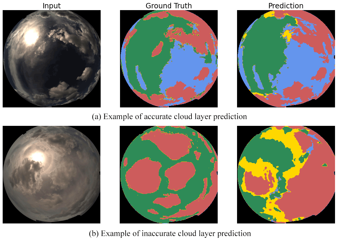
Figure 7Positive and negative prediction examples compared to ground truth for a given input from the validation set (blue: sky; red: low layer; yellow: mid-layer; green: high layer).
4.3 Comparison of binary segmentation results
Finally, we compare our approach to binary segmentation with the results of a state-of-the-art CSL (Kuhn et al., 2018). The dataset is the same as for previous evaluations, comprising 154 representative ASIs. Beforehand, our segmentation model (IP–SR*) was fine-tuned using binary ground truth masks, leading to slightly better results than postprocessing the semantic masks of four cloud types. Again we evaluated the models' pixel accuracy. Reaching 95.2 % on average, the CNN outperforms the CSL (87.9 %) by over 7 percentage points. As shown in Fig. 8, we also analyzed both methods under different predefined conditions of cloudiness, where the CNN always outmatches the CSL. Especially for more challenging mid- and high-layers clouds, our model achieves 90 %–95 %. In comparison to the CSL this a benefit of over 10 percentage points.
The binary cloud detection is a processing step at the beginning of most ASI applications, such as nowcasting. Hence, the increase in accuracy has the potential to improve the overall performance of these ASI applications significantly.
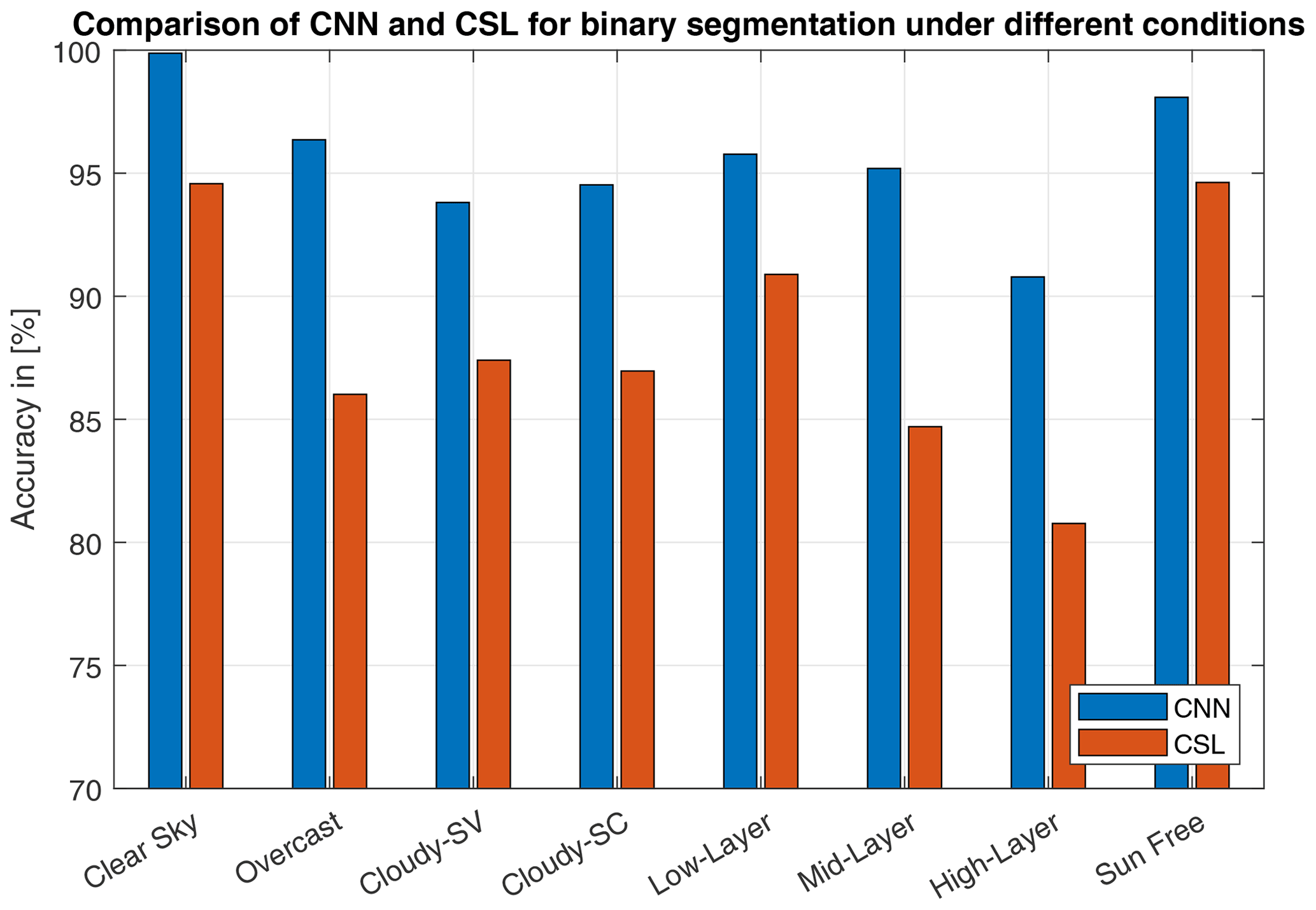
Figure 8Comparison of our results with a CSL for the validation set under different conditions of cloudiness. Cloudy-SV and Cloudy-SC specify partially clouded conditions with the sun visible (SV) or covered (SC). Sun Free determines whether the sun disk is completely free from clouds.
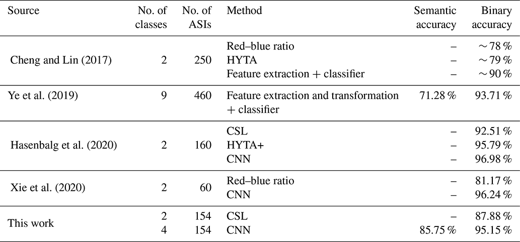
4.4 Comparing our results to the literature
In principle, an expressive comparison to the literature can only be conducted if the data for evaluation are the same. That is because prevailing cloud conditions within the dataset can be very different, and thus better or worse accuracies can be achieved. For example, the number of ASIs containing difficult cirrus clouds or atmospheric conditions with high Linke turbidity can affect the overall accuracies significantly. Still, the latest developments towards learning-based approaches show the superiority over traditional threshold-based methods, with our results confirming this trend (see Table 4). For instance, the proposed learning-based model from Cheng and Lin (2017) achieves over 10 percentage points more than a standard red–blue ratio or the HYTA (hybrid thresholding algorithm) model (Li et al., 2011). Also in other recent studies, machine learning models clearly outperform classical approaches like red–blue ratio, CSLs or the HYTA model.
Cheng and Lin (2017)Ye et al. (2019)Hasenbalg et al. (2020)Xie et al. (2020)Table 4Comparison of our results with the literature. Number of ASIs refers to the number of images used for validation.
In this paper, we presented the first approach to pretrain deep neural networks for ground-based sky observation using raw image data. Based on our results, these networks can be trained more effectively without the need for labeling thousands of images by hand. For cloud segmentation, this offers the possibility for simultaneously detecting and distinguishing clouds with associated properties in ASIs using deep learning. Our developed segmentation model is based on the U-Net architecture with a ResNet34 encoder, and the model categorizes ASI pixels into four classes. For self-supervised pretraining, we evaluated two distinct pretext tasks: inpainting–super-resolution and DeepCluster. We inspected the pretrained models' ability to solve their respective tasks and evaluated them for our validation set for cloud segmentation, containing 154 ASIs. By comparing the results from our pretrained models with the ones from ImageNet or random initialization, we showed the benefits of self-supervised learning. Considering only pixel accuracy, our pretrained models reach over 85 %, compared to 82.1 % (ImageNet initialization) and 78.3 % (random initialization). For mean IoU, the results are 80.5 %, 77.1 % and 72.1 %, respectively. But the most significant advantage becomes evident when regarding the distinction of cloud classes. In particular for more challenging cloud types such as mid- or high-layer clouds, precision, recall and IoU of the self-supervised models are often 10–20 percentage points higher. Furthermore, we evaluated our approach with regards to binary segmentation. Compared to a state-of-the-art CSL our model is more accurate under all examined conditions. On average accuracy is 95.2 % and thus 7 % higher than the accuracy of the CSL. Although an expressive comparison to the literature due to different datasets is not possible, our work confirms the superiority of learning-based approaches for cloud segmentation. However, there is still room for improvement in recognizing cloud types. High variability and similarity of different types make precise cloud classification difficult. In particular distant clouds and twilight zones cause false cloud type predictions. Therefore, more studies on other pretext tasks or other methods exploiting raw image data are needed. Finally, as self-supervised pretraining uses many more image data for training, it can be expected that the resulting models are more robust when being applied to other datasets. In particular, future models could be trained using large datasets of multiple cameras at different sites, potentially capable of generalizing well on any camera.
The underlying software code is property of the DLR and cannot be openly published.
The all-sky images and corresponding segmentation masks are property of the DLR's Institute of Solar Research and can be requested from the corresponding author (yann.fabel@dlr.de).
BN, SW, NB and YF conceived the presented idea. YF designed the models, performed the computations and analyzed the data. BN, SW, NB and RT verified the analytical methods and supervised the findings of this work. RT encouraged YF to investigate unsupervised learning methods. YF and MH contributed to the preparation of the dataset. PK and MH developed the reference clear-sky library. YF prepared the manuscript with contributions from all co-authors. RPP supervised the project.
The contact author has declared that neither they nor their co-authors have any competing interests.
Publisher’s note: Copernicus Publications remains neutral with regard to jurisdictional claims in published maps and institutional affiliations.
The German Federal Ministry for Economic Affairs and Energy funded this research within the WobaS-A project (grant agreement no. 0324307A). Further funding was received by the European Union within the H2020 program under the grant agreement no. 864337 (Smart4RES).
This research has been supported by the German Federal Ministry for Economic Affairs and Energy (grant no.
0324307A) and the European Union (grant no. 864337).
The article processing charges for this open-access publication were covered by the German Aerospace Center (DLR).
This paper was edited by Szymon Malinowski and reviewed by two anonymous referees.
Aitken, A., Ledig, C., Theis, L., Caballero, J., Wang, Z., and Shi, W.: Checkerboard artifact free sub-pixel convolution: A note on sub-pixel convolution, resize convolution and convolution resize, arXiv [preprint], arXiv:1707.02937, 2017. a
Blanc, P., Massip, P., Kazantzidis, A., Tzoumanikas, P., Kuhn, P., Wilbert, S., Schüler, D., and Prahl, C.: Short-term forecasting of high resolution local DNI maps with multiple fish-eye cameras in stereoscopic mode, AIP Conference Proceedings, 1850, 140004, https://doi.org/10.1063/1.4984512, 2017. a
Calbó, J., Long, C. N., González, J.-A., Augustine, J., and McComiskey, A.: The thin border between cloud and aerosol: Sensitivity of several ground based observation techniques, Atmos. Res., 196, 248–260, https://doi.org/10.1016/j.atmosres.2017.06.010, 2017. a
Caron, M., Bojanowski, P., Joulin, A., and Douze, M.: Deep clustering for unsupervised learning of visual features, in: Proceedings of the European Conference on Computer Vision (ECCV), pp. 132–149, https://doi.org/10.1007/978-3-030-01264-9_9, 2018. a, b, c, d
Chauvin, R., Nou, J., Thil, S., Traore, A., and Grieu, S.: Cloud detection methodology based on a sky-imaging system, Energy Proced., 69, 1970–1980, https://doi.org/10.1016/j.egypro.2015.03.198, 2015. a
Cheng, H.-Y. and Lin, C.-L.: Cloud detection in all-sky images via multi-scale neighborhood features and multiple supervised learning techniques, Atmos. Meas. Tech., 10, 199–208, https://doi.org/10.5194/amt-10-199-2017, 2017. a, b, c
Chow, C. W., Urquhart, B., Lave, M., Dominguez, A., Kleissl, J., Shields, J., and Washom, B.: Intra-hour forecasting with a total sky imager at the UC San Diego solar energy testbed, Sol. Energy, 85, 2881–2893, https://doi.org/10.1016/j.solener.2011.08.025, 2011. a
Cohn, S. A.: A New Edition of the International Cloud Atlas, WMO Bulletin, Geneva, World Meteorological Organization, 66, 2–7, 2017. a, b
Dev, S., Lee, Y. H., and Winkler, S.: Systematic study of color spaces and components for the segmentation of sky/cloud images, in: 2014 IEEE International Conference on Image Processing (ICIP), pp. 5102–5106, IEEE, https://doi.org/10.1109/ICIP.2014.7026033, 2014. a
Dev, S., Lee, Y. H., and Winkler, S.: Multi-level semantic labeling of sky/cloud images, in: 2015 IEEE International Conference on Image Processing (ICIP), pp. 636–640, IEEE, https://doi.org/10.1109/ICIP.2015.7350876, 2015. a
Dev, S., Wen, B., Lee, Y. H., and Winkler, S.: Machine learning techniques and applications for ground-based image analysis, arXiv [preprint], arXiv:1606.02811, 2016. a
Dev, S., Manandhar, S., Lee, Y. H., and Winkler, S.: Multi-label cloud segmentation using a deep network, in: 2019 USNC-URSI Radio Science Meeting (Joint with AP-S Symposium), pp. 113–114, IEEE, https://doi.org/10.1109/USNC-URSI.2019.8861850, 2019. a, b
Doersch, C., Gupta, A., and Efros, A. A.: Unsupervised visual representation learning by context prediction, in: Proceedings of the IEEE International Conference on Computer Vision, pp. 1422–1430, https://doi.org/10.1109/ICCV.2015.167, 2015. a
Ghonima, M. S., Urquhart, B., Chow, C. W., Shields, J. E., Cazorla, A., and Kleissl, J.: A method for cloud detection and opacity classification based on ground based sky imagery, Atmos. Meas. Tech., 5, 2881–2892, https://doi.org/10.5194/amt-5-2881-2012, 2012. a
Hasenbalg, M., Kuhn, P., Wilbert, S., Nouri, B., and Kazantzidis, A.: Benchmarking of six cloud segmentation algorithms for ground-based all-sky imagers, Sol. Energy, 201, 596–614, https://doi.org/10.1016/j.solener.2020.02.042, 2020. a, b, c, d
He, K., Zhang, X., Ren, S., and Sun, J.: Delving deep into rectifiers: Surpassing human-level performance on imagenet classification, in: Proceedings of the IEEE international conference on computer vision, pp. 1026–1034, https://doi.org/10.1109/ICCV.2015.123, 2015. a
He, K., Zhang, X., Ren, S., and Sun, J.: Deep residual learning for image recognition, in: Proceedings of the IEEE conference on computer vision and pattern recognition, pp. 770–778, https://doi.org/10.1109/CVPR.2016.90, 2016. a
Heinle, A., Macke, A., and Srivastav, A.: Automatic cloud classification of whole sky images, Atmos. Meas. Tech., 3, 557–567, https://doi.org/10.5194/amt-3-557-2010, 2010. a, b
Howard, J. and Ruder, S.: Universal language model fine-tuning for text classification, arXiv [preprint], arXiv:1801.06146, 2018. a
Howard, J. et al.: fastai, GitHub [code], https://github.com/fastai/fastai1 (last access: 10 February 2022), 2018. a
Ineichen, P. and Perez, R.: A new airmass independent formulation for the Linke turbidity coefficient, Sol. Energy, 73, 151–157, https://doi.org/10.1016/S0038-092X(02)00045-2, 2002. a
Ioffe, S. and Szegedy, C.: Batch normalization: Accelerating deep network training by reducing internal covariate shift, arXiv [preprint], arXiv:1502.03167, 2015. a
Jayadevan, V. T., Rodriguez, J. J., and Cronin, A. D.: A new contrast-enhancing feature for cloud detection in ground-based sky images, J. Atmos. Ocean. Tech., 32, 209–219, https://doi.org/10.1175/JTECH-D-14-00053.1, 2015. a
Jing, L. and Tian, Y.: Self-supervised visual feature learning with deep neural networks: A survey, IEEE Transactions on Pattern Analysis and Machine Intelligence, 43, 4037–4058, https://doi.org/10.1109/TPAMI.2020.2992393, 2020. a
Johnson, J., Alahi, A., and Fei-Fei, L.: Perceptual losses for real-time style transfer and super-resolution, in: European conference on computer vision, pp. 694–711, Springer, https://doi.org/10.1007/978-3-319-46475-6_43, 2016. a, b
Kazantzidis, A., Tzoumanikas, P., Bais, A. F., Fotopoulos, S., and Economou, G.: Cloud detection and classification with the use of whole-sky ground-based images, Atmos. Res., 113, 80–88, https://doi.org/10.1016/j.atmosres.2012.05.005, 2012. a
Kingma, D. P. and Ba, J.: Adam: A method for stochastic optimization, arXiv [preprint], arXiv:1412.6980 2014. a
Koren, I., Remer, L. A., Kaufman, Y. J., Rudich, Y., and Martins, J. V.: On the twilight zone between clouds and aerosols, Geophys. Res. Lett., 34, L08805, https://doi.org/10.1029/2007GL029253, 2007. a
Kuhn, P., Nouri, B., Wilbert, S., Prahl, C., Kozonek, N., Schmidt, T., Yasser, Z., Ramirez, L., Zarzalejo, L., Meyer, A., et al.: Validation of an all-sky imager–based nowcasting system for industrial PV plants, Progress in Photovoltaics: Research and Applications, 26, 608–621, https://doi.org/10.1002/pip.2968, 2018. a, b, c
Lee, H.-Y., Huang, J.-B., Singh, M., and Yang, M.-H.: Unsupervised representation learning by sorting sequences, in: Proceedings of the IEEE International Conference on Computer Vision, pp. 667–676, https://doi.org/10.1109/ICCV.2017.79, 2017. a
Li, Q., Lu, W., and Yang, J.: A hybrid thresholding algorithm for cloud detection on ground-based color images, J. Atmos. Ocean. Tech., 28, 1286–1296, https://doi.org/10.1175/JTECH-D-11-00009.1, 2011. a, b
Liu, S., Zhang, L., Zhang, Z., Wang, C., and Xiao, B.: Automatic cloud detection for all-sky images using superpixel segmentation, IEEE Geosci. Remote, 12, 354–358, https://doi.org/10.1109/LGRS.2014.2341291, 2014. a
Liu, S., Zhang, Z., Xiao, B., and Cao, X.: Ground-based cloud detection using automatic graph cut, IEEE Geosci. Remote, 12, 1342–1346, https://doi.org/10.1109/LGRS.2015.2399857, 2015. a
Long, C., Slater, D., and Tooman, T. P.: Total sky imager model 880 status and testing results, Pacific Northwest National Laboratory Richland, Wash, USA, https://doi.org/10.2172/1020735, 2001. a
Long, C. N., Sabburg, J. M., Calbó, J., and Pages, D.: Retrieving cloud characteristics from ground-based daytime color all-sky images, J. Atmos. Ocean. Tech., 23, 633–652, https://doi.org/10.1175/JTECH1875.1, 2006. a
Noroozi, M. and Favaro, P.: Unsupervised learning of visual representations by solving jigsaw puzzles, in: European Conference on Computer Vision, pp. 69–84, Springer, https://doi.org/10.1007/978-3-319-46466-4_5, 2016. a
Nouri, B., Wilbert, S., Kuhn, P., Hanrieder, N., Schroedter-Homscheidt, M., Kazantzidis, A., Zarzalejo, L., Blanc, P., Kumar, S., Goswami, N., Shankar, R., Affolter, R., and Pitz-Paal, R.: Real-time uncertainty specification of all sky imager derived irradiance nowcasts, Remote Sens., 11, 1059, https://doi.org/10.3390/rs11091059, 2019a. a
Nouri, B., Wilbert, S., Segura, L., Kuhn, P., Hanrieder, N., Kazantzidis, A., Schmidt, T., Zarzalejo, L., Blanc, P., and Pitz-Paal, R.: Determination of cloud transmittance for all sky imager based solar nowcasting, Sol. Energy, 181, 251–263, https://doi.org/10.1016/j.solener.2019.02.004, 2019b. a
Paszke, A., Gross, S., Massa, F., Lerer, A., Bradbury, J., Chanan, G., Killeen, T., Lin, Z., Gimelshein, N., Antiga, L., Desmaison, A., Kopf, A., Yang, E., DeVito, Z., Raison, M., Tejani, A., Chilamkurthy, S., Steiner, B., Fang, L., Bai, J., and Chintala, S.: PyTorch: An Imperative Style, High-Performance Deep Learning Library, in: Advances in Neural Information Processing Systems 32, edited by: Wallach, H., Larochelle, H., Beygelzimer, A., d'Alché-Buc, F., Fox, E., and Garnett, R., pp. 8024–8035, Curran Associates, Inc., http://papers.neurips.cc/paper/9015-pytorch-an-imperative-style-high-performance-deep-learning-library.pdf (last access: 10 February 2022), 2019. a
Pathak, D., Krahenbuhl, P., Donahue, J., Darrell, T., and Efros, A. A.: Context encoders: Feature learning by inpainting, in: Proceedings of the IEEE conference on computer vision and pattern recognition, pp. 2536–2544, https://doi.org/10.1109/CVPR.2016.278, 2016. a, b
Perez, R., David, M., Hoff, T. E., Jamaly, M., Kivalov, S., Kleissl, J., Lauret, P., and Perez, M.: Spatial and temporal variability of solar energy, Foundations and Trends in Renewable Energy, 1, 1–44, https://doi.org/10.1561/2700000006, 2016. a
Radford, A., Metz, L., and Chintala, S.: Unsupervised representation learning with deep convolutional generative adversarial networks, arXiv [preprint], arXiv:1511.06434, 2015. a
Ronneberger, O., Fischer, P., and Brox, T.: U-net: Convolutional networks for biomedical image segmentation, in: International Conference on Medical image computing and computer-assisted intervention, Springer, pp. 234–241, https://doi.org/10.1007/978-3-319-24574-4_28, 2015. a
Rossow, W. and Zhang, Y.-C.: Calculation of surface and top of atmosphere radiative fluxes from physical quantities based on ISCCP data sets: 2. Validation and first results, J. Geophys. Res.-Atmos., 100, 1167–1197, https://doi.org/10.1029/94JD02746, 1995. a
Rossow, W. B. and Schiffer, R. A.: Advances in understanding clouds from ISCCP, B. Am. Meteorol. Soc., 80, 2261–2288, https://doi.org/10.1175/1520-0477(1999)080<2261:AIUCFI>2.0.CO;2, 1999. a
Shelhamer, E., Long, J., and Darrell, T.: Fully convolutional networks for semantic segmentation, IEEE T. Pattern Anal., 39, 640–651, https://doi.org/10.1109/TPAMI.2016.2572683, 2017. a
Shi, C., Wang, Y., Wang, C., and Xiao, B.: Ground-based cloud detection using graph model built upon superpixels, IEEE Geosci. Remote, 14, 719–723, https://doi.org/10.1109/LGRS.2017.2676007, 2017. a
Shi, W., Caballero, J., Huszár, F., Totz, J., Aitken, A. P., Bishop, R., Rueckert, D., and Wang, Z.: Real-time single image and video super-resolution using an efficient sub-pixel convolutional neural network, in: Proceedings of the IEEE conference on computer vision and pattern recognition, pp. 1874–1883, https://doi.org/10.1109/CVPR.2016.207, 2016. a
Shields, J., Karr, M., Tooman, T., Sowle, D., and Moore, S.: The whole sky imager–a year of progress, in: Eighth Atmospheric Radiation Measurement (ARM) Science Team Meeting, Tucson, Arizona, pp. 23–27, Citeseer, 1998. a
Smith, L. N.: Cyclical learning rates for training neural networks, in: 2017 IEEE Winter Conference on Applications of Computer Vision (WACV), pp. 464–472, IEEE, https://doi.org/10.1109/WACV.2017.58, 2017. a
Smith, L. N.: A disciplined approach to neural network hyper-parameters: Part 1–learning rate, batch size, momentum, and weight decay, arXiv [preprint], arXiv:1803.09820, 2018. a
Song, Q., Cui, Z., and Liu, P.: An Efficient Solution for Semantic Segmentation of Three Ground-based Cloud Datasets, Earth Space Sci., 7, e2019EA001040, https://doi.org/10.1029/2019EA001040, 2020. a
Souza-Echer, M. P., Pereira, E. B., Bins, L., and Andrade, M.: A simple method for the assessment of the cloud cover state in high-latitude regions by a ground-based digital camera, J. Atmos. Ocean. Tech., 23, 437–447, https://doi.org/10.1175/JTECH1833.1, 2006. a
Stubenrauch, C., Rossow, W., Kinne, S., Ackerman, S., Cesana, G., Chepfer, H., Di Girolamo, L., Getzewich, B., Guignard, A., Heidinger, A., et al.: Assessment of global cloud datasets from satellites: Project and database initiated by the GEWEX radiation panel, B. Am. Meteorol. Soc., 94, 1031–1049, https://doi.org/10.1175/BAMS-D-12-00117.1, 2013. a
Taravat, A., Del Frate, F., Cornaro, C., and Vergari, S.: Neural networks and support vector machine algorithms for automatic cloud classification of whole-sky ground-based images, IEEE Geosci. Remote, 12, 666–670, https://doi.org/10.1109/LGRS.2014.2356616, 2014. a
West, S. R., Rowe, D., Sayeef, S., and Berry, A.: Short-term irradiance forecasting using skycams: Motivation and development, Sol. Energy, 110, 188–207, https://doi.org/10.1016/j.solener.2014.08.038, 2014. a
Widener, K. and Long, C.: All sky imager, uS Patent App. 10/377,042, 2004. a
Wilbert, S., Nouri, B., Prahl, C., Garcia, G., Ramirez, L., Zarzalejo, L., Valenzuela, R., Ferrera, F., Kozonek, N., and Liria, J.: Application of whole sky imagers for data selection for radiometer calibration, EU PVSEC 2016 Proceedings, pp. 1493–1498, https://doi.org/10.4229/EUPVSEC20162016-5AO.8.6, 2016. a
Xie, W., Liu, D., Yang, M., Chen, S., Wang, B., Wang, Z., Xia, Y., Liu, Y., Wang, Y., and Zhang, C.: SegCloud: a novel cloud image segmentation model using a deep convolutional neural network for ground-based all-sky-view camera observation, Atmos. Meas. Tech., 13, 1953–1961, https://doi.org/10.5194/amt-13-1953-2020, 2020. a, b
Ye, L., Cao, Z., and Xiao, Y.: DeepCloud: Ground-based cloud image categorization using deep convolutional features, IEEE T. Geosci. Remote, 55, 5729–5740, https://doi.org/10.1109/TGRS.2017.2712809, 2017. a
Ye, L., Cao, Z., Xiao, Y., and Yang, Z.: Supervised Fine-Grained Cloud Detection and Recognition in Whole-Sky Images, IEEE T. Geosci. Remote, 57, 7972–7985, https://doi.org/10.1109/TGRS.2019.2917612, 2019. a, b, c
Zhang, J., Liu, P., Zhang, F., and Song, Q.: CloudNet: Ground-based cloud classification with deep convolutional neural network, Geophys. Res. Lett., 45, 8665–8672, https://doi.org/10.1029/2018GL077787, 2018. a
Zhuo, W., Cao, Z., and Xiao, Y.: Cloud classification of ground-based images using texture–structure features, J. Atmos. Ocean. Tech., 31, 79–92, https://doi.org/10.1175/JTECH-D-13-00048.1, 2014. a
Centro de Investigaciones Energéticas, Medioambientales y Tecnológicas: a Spanish research institute with a focus on energy and environmental issues.