the Creative Commons Attribution 4.0 License.
the Creative Commons Attribution 4.0 License.
 | 15 Feb 2022
Characterizing and correcting the warm bias observed in Aircraft Meteorological Data Relay (AMDAR) temperature observations
Paul M. A. de Jong
Jitze van der Meulen
Some aircraft temperature observations, retrieved through the Aircraft Meteorological Data Relay (AMDAR), suffer from a significant warm bias when comparing observations with numerical weather prediction (NWP) models. In this paper we show that this warm bias of AMDAR temperature can be characterized and consequently reduced substantially. The characterization of this warm bias is based on the methodology of measuring temperature with a moving sensor and can be split into two separate processes.
The first process depends on the flight phase of the aircraft and relates to difference of timing, as it appears that the times of measurement of altitude and temperature differ. When an aircraft is ascending or descending, this will result in a small bias in temperature due to the (on average) presence of an atmospheric temperature lapse rate.
The second process is related to internal corrections applied to pressure altitude without feedback to temperature observation measurement.
Based on NWP model temperature data, combined with additional information on Mach number and true airspeed, we were able to estimate corrections using data over an 18-month period from January 2017 to July 2018. Next, the corrections were applied to AMDAR observations over the period from September 2018 to mid-December 2019. Comparing these corrected temperatures with (independent) radiosonde temperature observations demonstrates a reduction of the temperature bias from 0.5 K to around zero and a reduction of standard deviation of almost 10 %.
- Article
(1083 KB) - Full-text XML
- Companion paper
- BibTeX
- EndNote


Upper air observations from aircraft are an important source of information for numerical weather prediction (NWP) (Ingleby et al., 2021). Amongst other sources, aircraft observations of temperature and wind are used to estimate the atmospheric state in order to initialize an NWP forecast run. Knowledge about the error characteristics is crucial for correct interpretation of the observation. The presence of biases, which are persistent constant differences between observations and models, is detrimental to NWP performance (Dee and Da Silva, 1998). The European Centre for Medium-Range Weather Forecasts (ECMWF) has introduced an aircraft- and flight-phase-dependent temperature correction (Isaksen et al., 2012; Zhu et al., 2015; Ingleby et al., 2020). The so-called variational bias correction method (Dee, 2005) has been developed to remove the bias during assimilation, but the origin of the bias was not resolved.
In this paper the signature of the temperature bias from aircraft observations retrieved through the Aircraft Meteorological Data Relay (AMDAR) is investigated. These error characteristics of AMDAR temperature observations have been examined in a number of studies. A warm bias has been reported by Ballish and Kumar (2008). Drüe et al. (2007) observed aircraft-type-dependent systematic temperature errors. In general, the standard deviation of AMDAR minus radiosonde or AMDAR observations very close to each other is around 0.6 K (Schwartz and Benjamin, 1995; Benjamin et al., 1999).
In this paper the temperature bias is characterized, by assuming that the observed total bias consists of a flight phase part and a combined true airspeed and pressure-related part. Information available through the Mode-S Enhanced Surveillance system (EHS) is combined to characterize and quantize each dynamic part. The Mode-S EHS system on its own can be used to derive temperature as described in de Haan (2011). These observations of temperatures are not exploited here; instead the Mach number information and pressure altitude rate measured by an aircraft are used in the characterization. Temperatures from NWP are used to calibrate the bias for each aircraft individually as a function of true airspeed and pressure.
This paper is organized as follows: first we discuss briefly the aircraft sensors used and the origin of the data used to determine pressure and temperature, Mach and true airspeed. Next we present the (possible) sources of temperature biases and develop a methodology to quantify these biases. This section is followed by the description of the data preparation steps. The results are presented in Sect. 5, which is followed by the conclusions and discussion.
For flight control and aircraft management, modern aircraft are equipped with sensors which are used to derive basic meteorological parameters. A pitot probe measures static and total air pressure, and an immersion thermometer probe is installed for total air temperature measurements. The information is sent to the air data computer (ADC) to determine the actual state and share the information with other onboard systems, such as the Air Data Inertial Reference Unit (ADIRU). Some aircraft are equipped with other sensors which can measure humidity (mixing ratio) and/or sensors to detect the presence of ice on the flying surfaces. An inertial reference platform is part of the equipment for normal, longitudinal and lateral acceleration and rotations.
The Flight Management System (FMS) uses the information from the sensors for flight safety and cockpit information systems: modern aircraft are equipped with a positioning system which exploits the information from the Global Navigation Satellite System (GNSS). The FMS combines parameters to determine the position of the aircraft and complement the other sensors. For example, the Mach number is computed using static and total pressure measurements obtained by the pitot tube. The computed Mach number is then used in the derivation of the static air temperature from total air temperature. The true airspeed is in turn calculated using the Mach number and the total air temperature. Wind vector information is computed using the air vector (true airspeed and heading) and the ground vector (ground speed and track angle).
2.1 Mach number measurement
One of the basic instruments on an aircraft is the pitot tube, which is used to determine the Mach number by measuring the static pressure ps and dynamic pressure qi (which is the difference between static pressure ps and total air pressure pt, ). The Mach number is calculated as follows:
where γ is the ratio of specific heats of dry air (cp and cv).
The pressure measurements are deteriorated by the so-called pressure defect (Rodi and Leon, 2012), which is caused by flow disturbances around the sensor and depends on the angle of attack and the airspeed. Both total and static pressure suffer from this. The impact pressure is more accurate because it is the difference of the two.
The Mach number is the quotient of the true airspeed Va of the aircraft and the speed of sound c; . The speed of sound depends on the ambient static air temperature Ts (neglecting the small contribution of humidity) by
with R=287.05 J K−1 kg−1 the gas constant of dry air, ρ the density of the air; to estimate the true airspeed, temperature information is thus needed.
2.2 Aircraft temperature measurement
A thermometer probe measures the (total air) temperature Ti as it flies with a certain speed. This temperature is in general not equal to the static air temperature Ts due to the stagnation of the air and viscosity effects. The velocity difference between the probe and airflow causes a heating effect on the temperature element. When we assume that the flow is isentropic and is slowed down adiabatically to zero velocity, we have
where V is the velocity of the flow. The speed of sound can be written as
Then, if the energy transfer is (close to) adiabatic, the static air temperature is related to the measured temperature by (following WMO, 2018)
where M is the Mach number, and λ is the probe recovery factor, which includes the effect of viscosity and the effect of incomplete stagnation of air at the sensor. For the most common probe in service on commercial aircraft, λ=0.97, and given γ=1.4, the static air temperature becomes
2.3 AMDAR observations
Using the AMDAR system, a selection of the information which is available in the onboard computer can be transmitted to a ground station. The AMDAR software installed on the onboard computer collects and transmits the information through the Aircraft Communications Addressing and Reporting System (ACARS) system. In this way, wind and temperature observations can be received in almost real time, even from remote areas.
2.4 Mode-S EHS observations
Some information, available in the onboard computer (FMS and ADIRU), can be extracted from downlinked air traffic control (ATC) information using the secondary surveillance radar (SSR) technique Mode-S EHS. In the European designated EHS airspace, all fixed-wing aircraft, having a maximum take-off mass greater than 5700 kg or a maximum cruising true airspeed in excess of 125 m s−1 (approx. 250 kn), must be Mode-S EHS-compliant and should respond to the radar request. The set of parameters that can be downlinked consists of Mach number, air speed, indicated airspeed, magnetic heading and roll angle. In this study, the Mach number will be used to investigate the AMDAR temperature measurement accuracy. See de Haan (2011) for more details.
The Mode-S EHS data used in this study are kindly provided by EUROCONTROL and cover the airspace of Germany, Belgium, Luxembourg and the Netherlands.
2.5 Numerical weather prediction model data
The numerical weather prediction (NWP) model data used are from the operational non-hydrostatic model HIRLAM (Undén et al., 2002), which is run eight times per day with a 3DVAR assimilation cycle. AMDAR data are used in the assimilation, but to avoid problems in the comparison, a forecast with a lead time of at least 3 h is used. The NWP model-equivalent of the AMDAR temperature observation is determined by bilinear interpolation in the horizontal and linear interpolation in the logarithm of the pressure. A linear interpolation in time is performed between hourly space interpolated positions.
2.6 Parameter resolution and collocation method
In Table 1 the reported resolutions of time and position of AMDAR and Mode-S EHS are given. Apart from altitude, Mode-S EHS location parameters are reported at a higher resolution. In particular, the time resolution of AMDAR is low with respect to the altitude resolution. Note that the barometric altitude rate, the vertical speed of the aircraft, is not available in the AMDAR message.

The AMDAR and Mode-S EHS datasets are collocated as follows. The World Meteorological Organization (WMO) AMDAR aircraft identifier, provided in the reports, is linked with a ICAO 24-bit identifier using a lookup table. Next, within 300 s after an AMDAR observation, two Mode-S EHS observations are identified for which the pressure altitudes are closest, with one smaller and one larger than the AMDAR pressure altitude.
The lookup table has been provided by the EUMETNET AMDAR Programme Management for a number of aircraft; for the aircraft for which no official link between tail–number (or ICAO 24-bit identifier) is available, a collocation query has been applied. The result of this query is validated against the provided lookup table.
The temperature error can be influenced by several phenomena, such as airflow disturbances, incorrect calibration or sensor drift and inaccuracies of λ. Some of these phenomena are not easily quantified. In this paper it is assumed that the temperature error can be separated into a flight-phase-dependent, a Mach number and a (static) pressure-related part. The reference temperature used stems from NWP and has its own characteristics but is assumed to be flight-phase- and Mach-number-independent. In this section the methodology to determine the temperature bias characteristics from the observations is presented.
3.1 Flight-phase-dependent bias
It is observed that some aircraft exhibit a different bias when descending and ascending. Since average atmospheric profiles have a temperature lapse rate of K km K ft−1, this bias could be caused by time mis-synchronization between height message and the temperature message.
When the observation time of the temperature and the height differ, a bias will be introduced with opposite sign for descending and ascending flight paths. Suppose the time difference is τ, that is, when temperature T is observed at tT and the height at th, with , then
where v is the aircraft vertical speed. The height difference between reported height and height of the temperature is vτ, and thus a bias of Γvτ [K] will be present; that is
Inversely, when we know the vertical lapse rate and the temperature bias, we can estimate the time difference. The time difference is assumed to be the same for descending and ascending flight paths, and thus the bias due to the time difference is of opposite sign and different magnitude due to the difference in vertical velocity when descending or ascending. This implies that when the sum of the time difference biases is not equal to zero, an additional temperature bias may exist which is independent of the flight phase. This is most likely the case when the observation is compared to model temperatures because of representativeness, model orography and/or model parametrization.
Next, we estimate the time difference. Let τ be the time difference and vd and va be the descending and ascending vertical velocity, respectively. The observed descending and ascending temperatures Td and Ta will differ from the measured temperature T (without the time difference) as follows:
Suppose we have another observation of temperature Tref (e.g. from a numerical weather prediction model), which deviates from the AMDAR temperature T by
where β is the bias between AMDAR and the reference and ϵ the part of the temperature difference that cannot be described by β and which has a zero mean value. Let ΔT be the difference between observation and the reference; then
The time difference τ can be found as using many of collocated observations (in which case )
where denotes the mean value of parameter x. Finally, we correct the reference height of the temperature measurement using the vertical velocity of the aircraft.
3.2 Static pressure correction
The dynamic pressure qi is measured accurately, but the static pressure needs correction for angle of attack, airspeed and possibly other state variables (Rodi and Leon, 2012). Let be the uncorrected static pressure and the function f describe the correction of the static pressure; that is
The corrected ps is used to determine a corrected Mach number and true airspeed.
Because we observe that the temperature observation exhibits bias, we assume that this parameter is not recalculated using a corrected Mach number, and the observed temperature is calculated with the uncorrected pressure,
where is (uncorrected) biased temperature.
Suppose now that we can find an estimate of the inversion of correction function f; then together with an estimate the dynamic pressure qi deduced from indicated airspeed, we can estimate the impact temperature Ti by
and with the (corrected) Mach number, we can estimate the static air temperature as
Thus, when we have an estimate of the mapping f−1, we can correct the temperature measurement.
Suppose now that we have a set of collocated temperatures over a long period and full pressure range; then we might be able to find the inversion of the function f. Let Tc be the temperature used for calibration. Then f should obey
where
Figure 1 shows the value of f−1 as a function of ps and Va for a selected aircraft (filled contours) using NWP data over an 18-month period. As it turns out, the most dominant terms are related to pressure and true airspeed. The fit was constructed by binning both ps and Va in 10 separate bins, and we use the median value of f−1 in the least-squares fit. The function f−1 is approximated by
To avoid extreme values of b, we constrained b to the interval (0.8,1.2). We observe that the chosen representation of f−1 (contour lines) fits the data (filled contour).
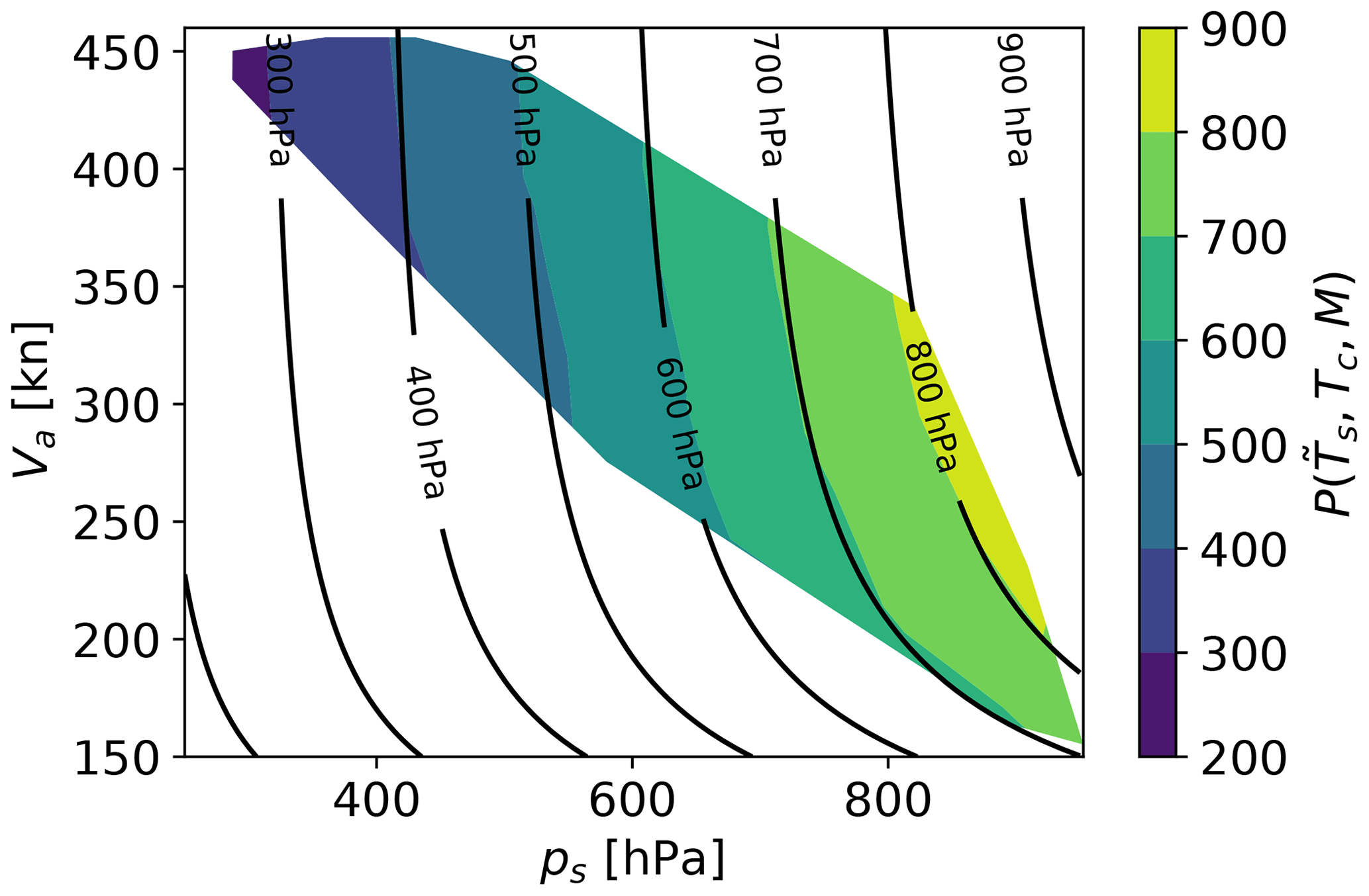
Figure 1Example of for an Airbus A321 aircraft (filled contour) and the approximation by f−1.
4.1 Estimation of correction coefficients
We collocated AMDAR temperature observatories with NWP for the period from 2 January 2017 to 31 July 2018. We used a forecast lead time of at least 3 h to avoid correlation due to assimilation of AMDAR. Next, the AMDAR observations are collocated with Mode-S EHS observations, where the height of observations is primarily used for collocating because the AMDAR time resolution is minutes, which is too coarse; the Mode-S EHS observations are linearly interpolated with respect to the AMDAR reported height. The observation time difference is at most 120 s. The fit is performed on binned data where the median values in bins are used. In this way we avoid over-fitting for pressure–airspeed values that occur more frequently than others. Furthermore, a minimum of 10 data points per bin was required.
4.2 Collocation with radiosonde observations
To show that the two correction methods have a positive effect on the measurement accuracy and bias of AMDAR temperatures, we compared the uncorrected and corrected values with independent observations. Over a period from 10 August 2018 to 17 December 2019, AMDAR observations are collocated with radiosonde observations. This period has no overlap with the period used to determine the correction coefficients. Radiosondes are generally considered to be a profile at one location and a single timestamp, but they are not. The time the balloon needs to reach 500 hPa is around 20 min, while the wind carries the platform over a distance of sometimes more than 100 km.
Radiosondes are generally launched 30 to 45 min before the main hours (00:00, 06:00, 12:00, 18:00 UTC), as required by WMO, with the majority of launches around 00:00 and 12:00 UTC (these timestamps represent the observation at a level of 500 hPa at the whole hour).
The dataset used was received over the Global Telecom System (GTS) and contains the operational available observations with a high resolution in reporting time (sometimes every second). All observations had a single timestamp which represents (or should represent) the moment the balloon reaches 500 hPa. The observation time was altered to take into account that the balloon rises with a vertical speed of approximately 5 m s−1. We did not include horizontal drift of the balloon.
An AMDAR observation is collocated with a radiosonde observation when the distance is smaller than 50 km, the time difference is smaller than 30 min and the height difference is less than 15 m. For each AMDAR observation, a nearby radiosonde observation, if it exists, was found. This implies that a radiosonde observation could have multiple matching AMDAR observations. This is reasonable for this study since we are interested in the quality of (corrected) AMDAR observations.
In this section we discuss the results of correcting AMDAR temperature observations by reconstruction of the uncorrected static pressure. The corrections are derived using NWP data over a period of 17 months (January 2017 to July 2018). The corrections are applied to AMDAR observations from the period September 2018 to December 2019. The (un)corrected temperatures are compared to radiosonde observations.
Both time periods and the source of information do not overlap and are independent implying a safe and sound comparison. Table 2 shows the result of the comparison. Clearly, the warm bias is diminished by applying both corrections. But not only has the bias improved, but the standard deviation also improves by almost 10 %. The magnitude of the standard deviation is higher than previously reported (0.6 K) because the collocation is less tight. The large difference in time and distance increases the standard deviation in particular.
Table 2Statistics of uncorrected AMDAR temperature observations (raw) minus radiosonde temperature observations, for the period 17 September 2018 to 17 December 2019. Statistics of corrected AMDAR: only flight phase correction (τ), only pressure correction (ps) and both corrections applied (τ,ps). The corrections are estimated using NWP and Mode-S EHS from the period 2 January 2017 to 31 July 2018. The number of collocated data points is 14 716.
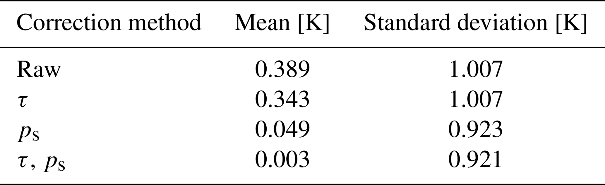
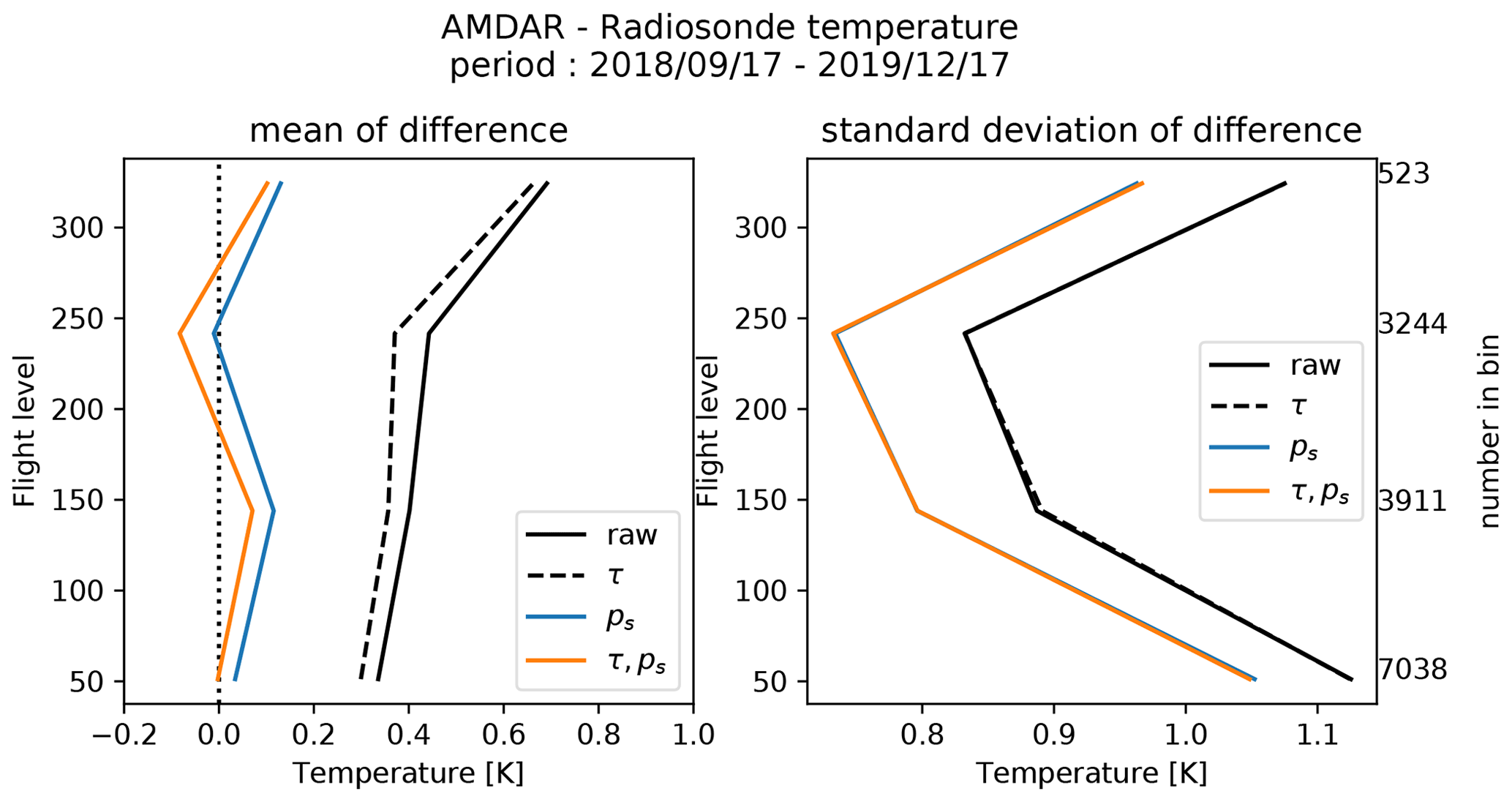
Figure 2 shows the mean difference (left panel) and standard deviation of the difference (right panel) with respect to flight level. Over the whole atmospheric profile, the bias and standard deviation improve significantly when the corrections are applied. Note that the numbers on right panel denote the number of data points in each vertical bin.
The peak of standard deviation near the surface is related to natural variability of temperature and the fact that both measurement systems are not completely collocated. The larger standard deviation near the top could be related to a low number of data points and general measurement inaccuracies of the aircraft temperature measurement.
Figure 3 shows four panels with profile statistics for the main synoptic hours. The left-most panel shows that at 00:00 UTC, after correction, the bias has an almost constant but small positive value. The right-most panel (18:00 UTC) has the most positive bias below flight level 150. The bias is around zero for 12:00 UTC observations The reason for the difference in bias with the time of day is not understood. Assuming that the AMDAR bias is constant, we observe that the radiosonde bias changes over the day from overestimation at 06:00 UTC to neutral at 12:00 UTC and underestimation at 18:00 UTC to slight underestimation at 00:00 UTC. Note that the number of aircraft observations around 00:00 UTC is dramatically lower than around 12:00 UTC, which influences the significance of the bias. Further research with a longer dataset is needed to investigate this.
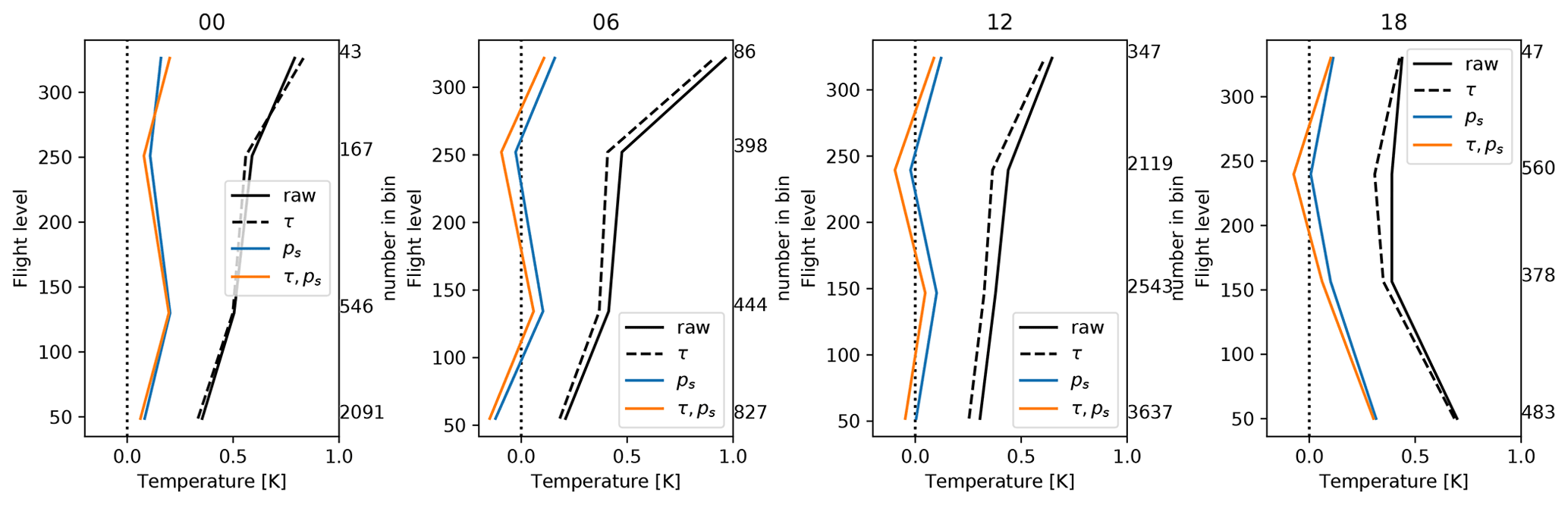
Figure 3Mean of AMDAR temperature minus radiosonde temperature, subdivided into 4 synoptic hours.
Figure 4 shows the mean (left panel) and standard deviation (right panel) of the difference between AMDAR and radiosonde temperature observations grouped by aircraft type. A minimum threshold of 10 observations per aircraft is required. For all but three aircraft types, the bias is reduced. For (a single) A30B we observe that the bias changes sign, for the 7 A388 aircraft we observe no change and for the 2 B736 a slight increase is observed. The reduction in bias for aircraft with large biases is very large. With respect to the standard deviation, all observed standard deviations are equal or smaller with corrections applied.
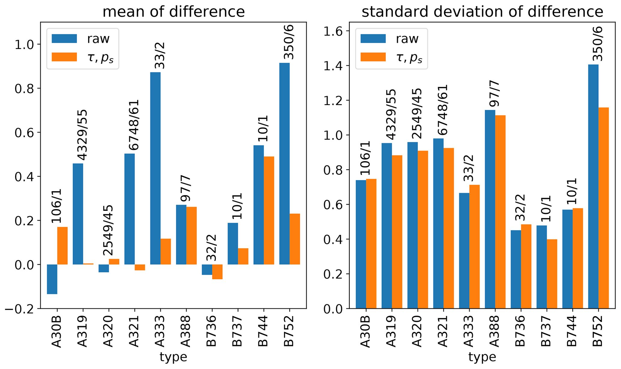
Figure 4Bias and standard deviation of AMDAR minus radiosonde temperatures, grouped by aircraft type. The two numbers for each group denote the total number of observations and the number of unique aircraft, respectively.
In this paper we demonstrated that the AMDAR warm bias can be characterized by two methods of corrections: the first is a timing-related correction, while the second relates to the interconnected nature of pressure, Mach and temperature measurements. Both corrections can be found using an external source of temperature information, together with Mode-S EHS downlinked parameters, such as true airspeed and Mach number.
In this paper we used NWP data to characterize the corrections. Also, the corrected AMDAR temperatures were compared to radiosonde observations but for a different period, so that this comparison was completely independent. As a consequence the resulting bias was diminished by the correction, while the standard deviation reduced by almost 10 %.
Both corrections are currently assumed to be constant and static in time. To assure model or source independence, a different dataset in time is required to construct the correction parameters (τ, a, b and c). Further research, including a longer time period, is required to verify that this constant assumption is valid since one can expect that aircraft maintenance can affect the time synchronization or static pressure corrections. This could also explain the results for the two aircraft showing increased bias in our results.
The Mode-S EHS information can be applied to correct the AMDAR temperature bias, for those air spaces where Mode-S EHS information is available. However, this is not a long-term solution. It would be better if the corrections are applied at the source, that is, in the avionics.
The code will be made available in due time through the Internet website https://emaddc.com/default.aspx (last access: 15 January 2022).
Mode-S EHS data will be made available as open data through the website https://emaddc.com/default.aspx (last access: 15 January 2022; European Meteorological Aircraft Derived Data Centre, 2022). Access to AMDAR data is restricted to the Meteorogical community. ECMWF data can be downloaded from http://ecmwf.int (last access: 15 January 2022; European Centre for Medium-Range Weather Forecasts, 2022).
The main research was carried out by SdH. PMAdJ's contribution was mainly related to Mode-S, while JvdM's contribution was on AMDAR.
The contact author has declared that neither they nor their co-authors have any competing interests.
Publisher’s note: Copernicus Publications remains neutral with regard to jurisdictional claims in published maps and institutional affiliations.
The authors would like to thank the Eumetnet AMDAR Programme Management for providing the aircraft identifier lookup table. The Mode-S EHS data used in this study have kindly been provided by EUROCONTROL, Maastricht Upper Area Control.
This paper was edited by Piero Di Carlo and reviewed by Mikhail Strunin and two anonymous referees.
Ballish, B. A. and Kumar, K. V.: Systematic Differences in Aircraft and Radiosonde Temperatures, B. Am. Meteorol. Soc., 89, 1689–1707, https://doi.org/10.1175/2008bams2332.1, 2008. a
Benjamin, S. G., Schwartz, B. E., and Cole, R. E.: Accuracy of ACARS Wind and Temperature Observations Determined by Collocation, Weather Forecast., 14, 1032–1038, https://doi.org/10.1175/1520-0434(1999)014<1032:AOAWAT>2.0.CO;2, 1999. a
Dee, D. P.: Bias and data assimilation, Q. J. Roy. Meteor. Soc., 131, 3323–3343, https://doi.org/10.1256/qj.05.137, 2005. a
Dee, D. P. and Da Silva, A. M.: Data assimilation in the presence of forecast bias, Q. J. Roy. Meteor. Soc., 124, 269–295, https://doi.org/10.1002/qj.49712454512, 1998. a
de Haan, S.: High-resolution wind and temperature observations from aircraft tracked by Mode-S air traffic control radar, J. Geophys. Res., 116, D10111, https://doi.org/10.1029/2010JD015264, 2011. a, b
Drüe, C., Frey, W., Hoff, A., and Hauf, T.: Aircraft type-specific errors in AMDAR weather reports from commercial aircraft, Q. J. Roy. Meteor. Soc., 134, 229–239, https://doi.org/10.1002/qj.205, 2007. a
European Centre for Medium-Range Weather Forecasts (ECMWF): https://www.ecmwf.int/, last access: 27 January 2022. a
European Meteorological Aircraft Derived Data Centre (EMADDC): https://emaddc.com/default.aspx, last access: 27 January 2022. a
Ingleby, B., Isaksen, L., and Kral, T.: Evaluation and impact of aircraft humidity data in ECMWF's NWP system, ECMWF, ECMWF Technical Memoranda No. 855, https://doi.org/10.21957/4e825dtiy, 2020. a
Ingleby, B., Candy, B., Eyre, J., Haiden, T., Hill, C., Isaksen, L., Kleist, D., Smith, F., Steinle, P., Taylor, S., Tennant, W., and Tingwell, C.: The Impact of COVID-19 on Weather Forecasts: A Balanced View, Geophys. Res. Lett., 48, e2020GL090699, https://doi.org/10.1029/2020GL090699, 2021. a
Isaksen, L., Vasiljevic, D., Dee, D., and Healy, S.: Bias correction of aircraft data implemented in November 2011, ECMWF, ECMWF Newsletter, 131, p. 6, 2012. a
Rodi, A. R. and Leon, D. C.: Correction of static pressure on a research aircraft in accelerated flight using differential pressure measurements, Atmos. Meas. Tech., 5, 2569–2579, https://doi.org/10.5194/amt-5-2569-2012, 2012. a, b
Schwartz, B. E. and Benjamin, S. G.: A Comparison of Temperature and Wind Measurements from ACARS-Equipped Aircraft and Rawinsondes, Weather Forecast., 10, 528–544, https://doi.org/10.1175/1520-0434(1995)010<0528:ACOTAW>2.0.CO;2, 1995. a
Undén, P., Rontu, L., Järvinen, H., Lynch, P., Calvo, J., Cats, G., Cuxart, J., Eerola, K., Fortelius, C., Garcia-Moya, J., Jones, C., Lenderlink, G., McDonald, A., McGrath, R., Navascues, B., Nielsen, N., Odegaard, V., Rodriguez, E., Rummukainen, M., Room, R., Sattler, K., Sass, B., Savijärvi, H., Schreur, B., Sigg, R., The, H., and Tijm, A.: HIRLAM-5 Scientific Documentation, Tech. rep., HIRLAM-project, Norrköping, available at: http://hirlam.org/ (last access: 28 December 2021), 2002. a
WMO: Guide to Instruments and Methods of Observation, Volume III: Observing Systems, available at: https://library.wmo.int/ (last access: 28 December 2021), 2018. a
Zhu, Y., Derber, J. C., Purser, R. J., Ballish, B. A., and Whiting, J.: Variational Correction of Aircraft Temperature Bias in the NCEP's GSI Analysis System, Mon. Weather Rev., 143, 3774–3803, https://doi.org/10.1175/MWR-D-14-00235.1, 2015. a