the Creative Commons Attribution 4.0 License.
the Creative Commons Attribution 4.0 License.
 | 23 Feb 2022
Assessing synergistic radar and radiometer capability in retrieving ice cloud microphysics based on hybrid Bayesian algorithms
Yuli Liu
Gerald G. Mace
The 2017 National Academy of Sciences Decadal Survey highlighted several high-priority objectives to be pursued in the decadal timeframe, and the next-generation Cloud, Convection and Precipitation (CCP) observing system is thereby contemplated. In this study, we develop a suite of hybrid Bayesian algorithms to evaluate two CCP remote sensor candidates including a W-band cloud radar and a (sub)millimeter-wave radiometer with channels in the 118–880 GHz frequency range for capability in constraining ice cloud microphysical quantities. The algorithms address active-only, passive-only, and synergistic active–passive retrievals. The hybrid Bayesian algorithms combine the Bayesian Monte Carlo integration and optimization process to retrieve quantities with uncertainty estimates. The radar-only retrievals employ the optimal estimation methodology, while the radiometer-involved retrievals employ ensemble approaches to maximize the posterior probability density function. A priori information is obtained from the Tropical Composition, Cloud and Climate Coupling (TC4) in situ data and CloudSat radar observations. End-to-end simulation experiments are conducted to evaluate the retrieval accuracies by comparing the retrieved parameters with known values. The experiment results suggest that the radiometer measurements possess high sensitivity to ice cloud particles with large water content. The radar-only retrievals demonstrate capability in reproducing ice water content profiles, but the performance in retrieving number concentration is poor. The synergistic observations enable improved pixel-level retrieval accuracies, and the improvements in ice water path retrievals are significant. The proposed retrieval algorithms could serve as alternative methods for exploring the synergistic active and passive concept, and the algorithm framework could be extended to the inclusion of other remote sensors to further assess the CCP observing system in future studies.
- Article
(2951 KB) - Full-text XML
- BibTeX
- EndNote


The 2017 National Academy of Sciences Decadal Survey (National Academies of Sciences, Engineering, and Medicine, 2018) identified five designated foundational observations to be pursued during the 2017–2027 time frame, including aerosols (A), clouds, convection, and precipitation (CCP) as designated observables (DOs). In the preformulation study, the A and CCP DOs were merged to exploit synergies in the measurement systems. The objective of the preformulation study was to identify measurables that can achieve the science objectives of the DOs. As such, the study identified observing system architectures that maximize science benefits while limiting cost and risk. To narrow in on a set of viable architectures, the ACCP study relied on a suite of observing system simulation experiments (OSSEs) aimed at addressing pixel-level retrieval uncertainties and sampling trade-offs for various geophysical variables that were deemed important for achieving science goals.
The properties of ice clouds are among the critical geophysical variables in the CCP science objectives. Ice clouds play a significant role in modulating the energy budget of the earth system by absorbing upwelling long-wave radiation emitted from the lower troposphere and reflecting incoming solar short-wave radiation (Liou, 1986). Studies suggest that ice clouds are a net heat source to the climate system (Ackerman et al., 1988; Berry and Mace, 2014) while contributing positive feedback to the climate system (Zelinka and Hartmann, 2011).
The radiative effects of ice clouds depend on the vertically integrated quantities and the vertical distribution of ice particle characteristics (Hartmann and Berry, 2017). The microwave radar and (sub)millimeter-wave radiometry are two critical techniques for ice cloud remote sensing and they are strongly complementary when combined (Buehler et al., 2012). The microwave radar reflectivity constrains ice cloud microphysical quantities in a vertically resolved sense while the (sub)millimeter-wave radiometer constrains integrated mass and particle size. Further, the nadir-looking microwave cloud radar provides high-resolution vertical profiles of ice clouds but is limited to the along-track measurements, whereas the scanning (sub)millimeter-wave radiometer has a wide swath but provides limited information about cloud vertical structure. Combing the strength of both observing sensors enhances our capability to better acquire ice cloud spatial distributions and assess their role in radiative heating.
Several retrieval algorithms have been developed specifically for ice cloud radiometry studies. All applicable algorithms that could be generally classified as statistical approaches and optimization approaches are under the framework of Bayes’ theorem. The statistical approaches, including the Bayesian Monte Carlo integration (MCI) (Evans et al., 2002, 2005) and the neural network (Jiménez et al., 2007; Brath et al., 2018), build an a priori database by randomly generating atmospheric/cloud cases according to the a priori probability density function (PDF) and simulating instrument-specific measurements. To solve the sparsity of database cases in the measurement space, optimization algorithms were developed to maximize the posterior PDF. Evans et al. (2012) applied the optimal estimation method (OEM) and Markov chain Monte Carlo (MCMC) method to retrieve ice cloud profiles from the Compact Scanning Submillimeter Imaging Radiometer (CoSSIR) (Evans et al., 2005) observations during the Tropical Composition, Cloud and Climate Coupling (TC4) (Toon et al., 2010) experiment. Liu et al. (2018) proposed an ensemble methodology that does not use the gradient information but always relies on estimating posterior PDF to minimize the cost function. For the combined radar and radiometer retrievals, McFarlane et al. (2002) explored the synergistic concepts by retrieving liquid water content and effective radius profiles from millimeter-wavelength radar reflectivity and dual-channel microwave brightness temperatures (BTs) using the Bayesian MCI algorithm. Although McFarlane et al. (2002) worked on the liquid cloud, the basic methodologies are applicable to the ice cloud remote sensing. Pfreundschuh et al. (2020) developed OEM algorithms for the upcoming Ice Cloud Imager radiometer (Kangas et al., 2014) and a conceptual W-band cloud radar to investigate synergies between the active and passive observations.
The objective of this paper is to develop candidate retrieval algorithms for synergistic radar and radiometer observations in order to quantitatively assess the capability of the next-generation ACCP observing system in constraining ice cloud geophysical variables. The algorithms for active-only, passive-only, and synergistic retrievals are developed under a hybrid Bayesian framework that combines the Bayesian MCI and optimization process to retrieve ice cloud quantities with uncertainty estimates. This paper is structured as follows: in Sect. 2 we provide an overview of the candidate ACCP remote sensors and present the simulated active and passive observations on the reference cloud scenes using the radiative transfer model. Section 3 describes the hybrid Bayesian algorithms for the radar-only, radiometer-only, and synergistic retrievals in detail, followed by Sect. 4, which describes the retrieval database using the statistics from in situ data and CloudSat radar observations. Section 5 presents the retrieval simulation experiments and a quantitative evaluation of the retrieval results. Finally, Sect. 6 presents the summary and conclusions.
2.1 Remote sensors
The remote sensors we evaluate in this study include a W-Band (94.05 GHz) radar and a (sub)millimeter-wave radiometer both of which are candidates in the ACCP observing system. The W-band radar is nadir-looking and it is similar to the Cloud Profiling Radar (CPR) in the CloudSat satellite (Stephens et al., 2008). The radar’s horizontal resolutions are 1 and 0.8 km in along-track and cross-track directions, respectively. The reflectivity measurement accuracy is 1.5 dBz, and the minimum detectable reflectivity is −25 dBz when working in high-sensitivity mode. The passive (sub)millimeter-wave radiometer is conical-scanning and it has 16 horizontally polarized channels at the frequencies of 118±1.1, 118±1.5, 118±2, 118±5, 183±1, 183±2, 183±3, 183±6, 240, 310, 380±0.75, 380±1.5, 380±3, 380±6, 660, and 880 GHz. The 183 and 380 GHz channels are centered around water vapor absorption lines, and the other channels are centered around the O2-line or within the window region. The desired radiometric resolution and the spectral feature for different channels of this candidate radiometer are summarized in Table 1 based on the information disclosed on https://aos.gsfc.nasa.gov (last access: 18 February 2022). The noise characteristic for the 310 GHz channel is not specified, and it is assumed to be 1.5 K in this study. The radiometer has a 45∘ off-nadir angle and a 750 km swath width. The assumptions used in this study align with the assumed instruments that were used in the ACCP study. Specific instruments have yet to be chosen and therefore additional details regarding the actual flight instruments are not known. Figure 1 shows the simulated clear-sky BT spectrum for a tropical atmospheric profile. All channels of the ACCP candidate (sub)millimeter-wave radiometer are positioned on the spectrum, and detailed views of the double sidebands located on either side of the central frequency are also displayed.
This study focuses on developing synergistic retrieval algorithms for situations where the active and passive observations are coincident. Based on this purpose, although the radar and radiometer instruments have different horizontal resolution and scanning modes, both sensors are assumed to have the same nadir-looking pencil beam and the capacity of high horizontal resolution to achieve the same fields of view in the simulation experiments below. The influence of the footprint and viewing geometry will be addressed in future work once more characteristics are known.
Table 1Channel characteristics of the ACCP candidate (sub)millimeter-wave radiometer based on the information disclosed on https://aos.gsfc.nasa.gov (last access: 18 February 2022).
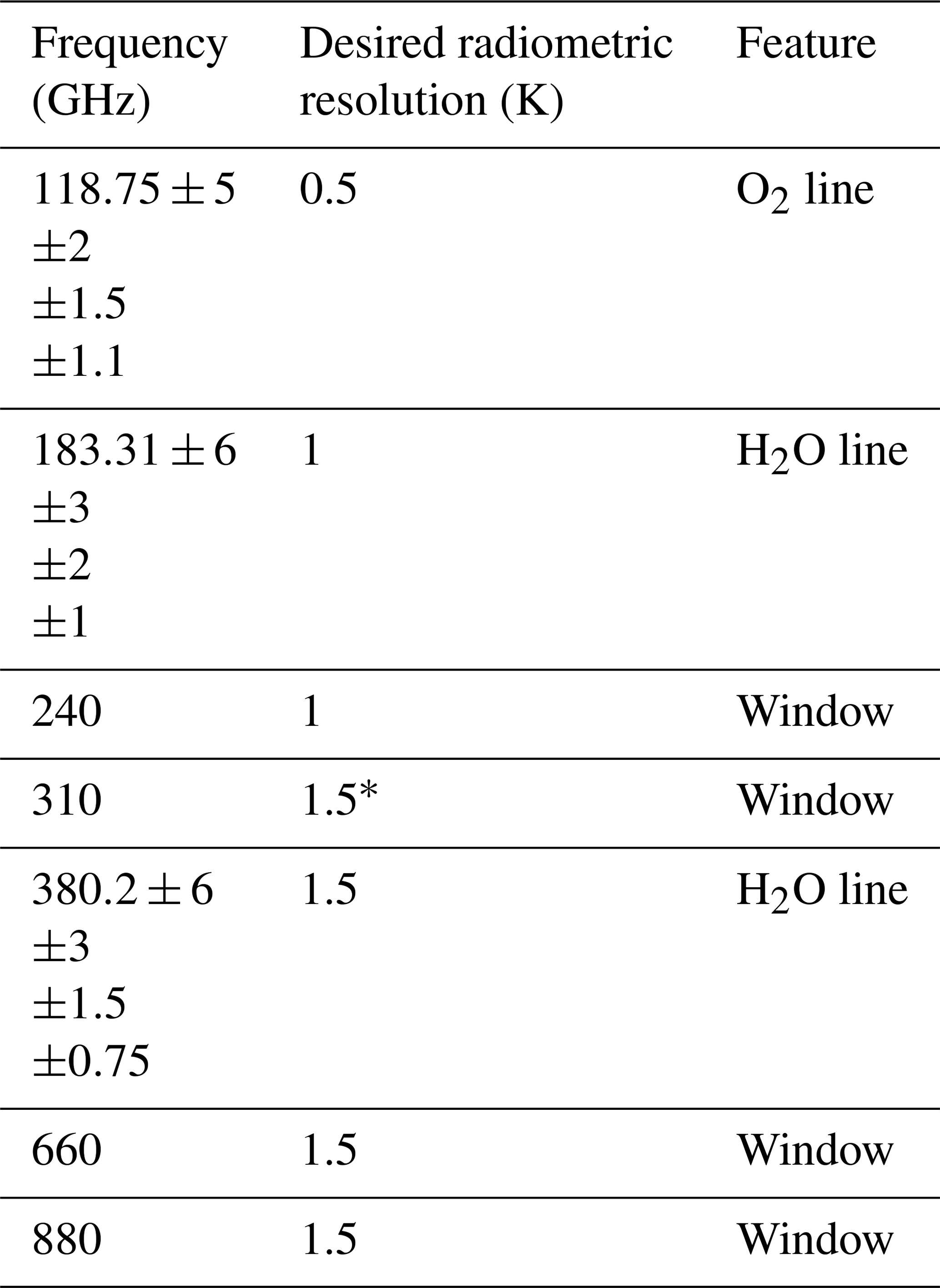
* The noise quantity for the 310 GHz channel is not specified, and it is assumed to be 1.5 K in this study.
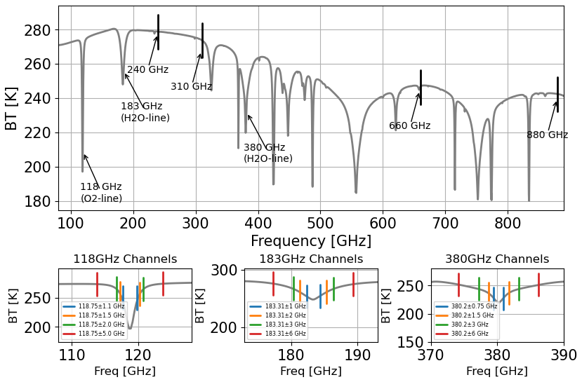
Figure 1Simulated clear-sky brightness temperature spectrum in a tropical atmospheric scenario. All ACCP radiometer channel positions and a detailed view of the double sidebands located on either side of a central frequency are present.
2.2 Reference cloud scenes
The reference cloud scenes are obtained from the numerical Environment and Climate Change Canada (ECCC) model (Chen et al., 2020) simulating tropical atmospheric conditions. The ECCC model outputs were made available to the ACCP Science Impacts Team (Pavlos Kollias, personal communication, 2019) and were originally created for use by the EarthCARE Algorithm Team (Illingworth et al., 2015). The intent to choose the ECCC atmosphere/cloud profiles is to assure the independence between the ice cloud microphysics for reference and that in the retrieval database, but also to keep these two datasets consistent in a geographic context. As will be discussed in Sect. 4, the a priori database is created using in situ statistics from the NASA TC4 campaign that occurred in the Tropical Eastern Pacific. The ECCC model outputs water content and number concentration (NC) profiles for several types of hydrometer including cloud ice, snow, liquid cloud, and rain. In this study, however, we only use the frozen particle outputs, and we do not differentiate between cloud ice and snow but add the water content and NC of these two hydrometer species to parameterize the frozen particles. The reason for these simplifications is still to be consistent with the a priori database that will be discussed in Sect. 4. Currently, the retrieval database we create does not contain liquid hydrometeors, and we do not distinguish between cloud ice and snow when analyzing the TC4 in situ data to capture the a priori statistics. All ECCC model outputs are interpolated according to the CloudSat CPR range gate spacing that has 250 m vertical resolutions to mimic realistic remote sensing situations. A total of 1280 atmosphere/cloud profiles with 0.25 km horizontal resolution along a latitudinal transect between −2.5 and 9∘ latitude are selected as the reference cloud profiles for assessing the retrieval accuracies of the remote sensors studied.
2.3 Radiative transfer model
We develop the one-dimensional forward model for both active and passive simulations based on the Atmospheric Radiative Transfer Simulator (ARTS) (Buehler et al., 2018). The ARTS forward model used in this study employs the built-in two-moment modified gamma distribution (Petty and Huang, 2011) scheme, which requires both ice water content (IWC) and NC to characterize the frozen particle size distribution (PSD). The frozen particles are assumed to be randomly orientated, and their scattering properties are represented by the “EvansSnowAggregate” particle habit in the ARTS Single Scattering Database (SSD) (Eriksson et al., 2018). The ARTS model uses a single-scattering radar solver to compute the radar reflectivity, and it uses the DIScrete Ordinates Radiative Transfer (DISORT) (Stamnes et al., 2000) solver to compute the BT. The gas absorptions are computed using the HITRAN database (Rothman et al., 2013), and the surface emissivity is calculated using the Tool to Estimate Sea-Surface Emissivity from Microwaves to sub-Millimeter Wave (TESSEM) (Prigent et al., 2017) emissivity model. It should be noted that the ARTS forward models used in simulating observations of the reference cloud scenes are identical to the models used in the optimization retrieval algorithms, which means the systematic biases from different particle habits or PSD schemes are not investigated in this study.
2.4 Simulated observations
Figure 2 shows the vertical distribution of IWC and NC for the selected reference cloud scenes along a latitudinal transect and the corresponding simulated W-band radar reflectivity observations. Compared to the NC, the radar reflectivity simulations show a stronger tendency to follow the variations of IWC. Figure 3 shows the ice water path (IWP) and the corresponding BT simulations for different channels of the ACCP candidate radiometer. The correlations between the IWP changes and BT depressions are evident. The channels with higher central frequencies are more sensitive to the change of the water path, especially when the IWP is around 102 g m−2. For the double sidebands with the same center frequency, the large frequency-offset channels show higher BT values in clear-sky conditions, and they have larger BT depressions when encountering thick ice cloud layers. Figure 4 shows the scatterplot of the BT difference between simulations in the clear-sky and cloudy conditions versus IWP for different channels. The 118 GHz channels demonstrate sensitivity only when the IWP is over 103 g m−2. This is not surprising since the 118 GHz channels are primely designed for sensing temperature profiles. For the 183 and 380 GHz channels, the biggest BT differences are up to 50 and 80 K, respectively. Also, the 380 GHz channels simulations show more deviations for the same IWP values, implying that the high-frequency channels are more sensitive to the IWC vertical distributions. The BT sensitivity of the 660 and 880GHz window channels are noticeable even when the IWP is below 102 g m−2, and the difference in values could be up to 110 K under our reference cloud scenes. These two channels make the candidate radiometer capable of sensing thin cirrus clouds that are usually composed of smaller particles. However, both 660 and 880 GHz show signs of saturation for IWP in excess of 103 g m−2 explaining why the full suite of channels is necessary to capture the full dynamic range of ice clouds in the upper troposphere.
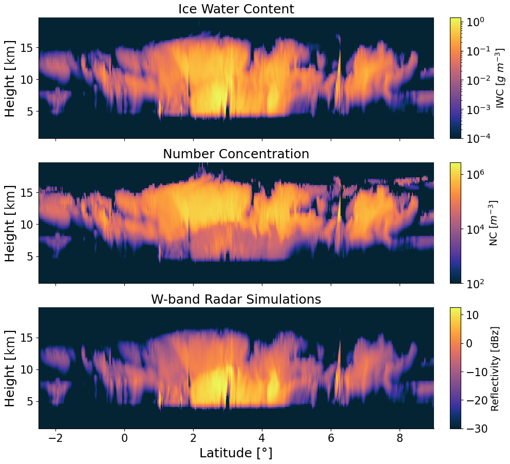
Figure 2Vertical distribution of water content (WC) and number concentration (NC) for ice and snow particles along the selected latitudinal transact and the corresponding W-band radar reflectivity simulations. The radar simulations are computed using the Atmospheric Radiative Transfer Simulator (ARTS) forward model.

Figure 3Integrated ice cloud water content of the selected latitudinal transect and the corresponding brightness temperature simulations for the candidate ACCP radiometer's channels.
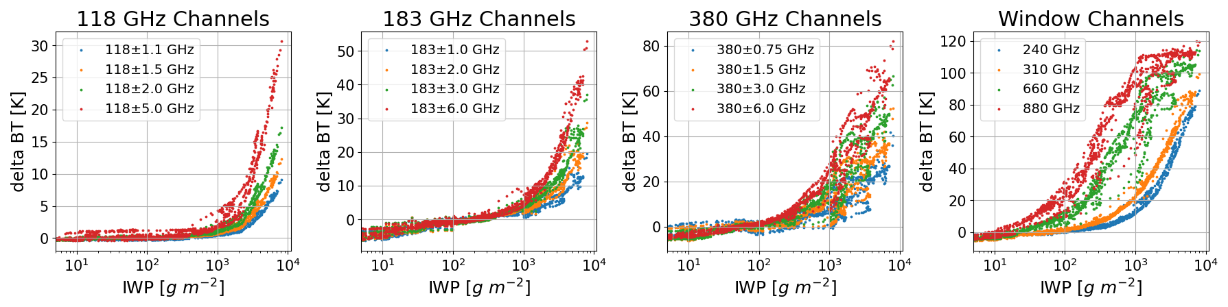
Figure 4Scatterplot of the brightness temperature difference between simulations in the clear-sky and cloudy conditions as a function of ice water path for all ACCP radiometer channels.
We developed different hybrid Bayesian algorithms for the radar-only, radiometer-only, and synergistic retrievals. All hybrid algorithms combine Bayesian MCI with optimization processes to retrieve quantities and uncertainty estimates. Bayesian MCI introduces prior information by generating an ensemble of atmospheric cases that are distributed according to the a priori PDF, and it is highly efficient since the retrieval database is precalculated and additional forward model calculations are not required. By assuming the uncertainties for different measurement variables to be independent, the conditional PDF can be written as (Evans et al., 2002):
where Pcond is the conditional probability of the measurement vector yobs given a particular atmospheric state x, ysim is the simulated observation vector, and σj is the uncertainty of observation and forward model for the jth channel. The retrieved quantities and uncertainties are calculated by MCI over the state vectors to find the mean vector and the associated standard deviation (Evans et al., 2002):
The biggest challenge for the Bayesian MCI is the sparsity in the measurement space for a retrieval database with a finite number of random samples. If we increase the length of the observation vector or decrease the measurement uncertainties, the number of database cases matching the observation vector becomes smaller and the Bayesian MCI fails. When this happens, the optimization process is begun to maximize the posterior PDF.
3.1 Radar-only retrievals
The robust and efficient OEM method is employed as the optimization algorithm for radar-only retrievals. The fundamental assumptions of the OEM algorithm are that the forward model is moderately nonlinear and that both the prior PDF and conditional PDF are Gaussians. OEM maximizes the posterior PDF by minimizing the following cost function (Rodgers, 2000):
where Sy and Sa are the covariance matrices for the measurement and prior uncertainties, respectively. In this study, the Levenberg–Marquardt minimization method (Rodgers, 2000) is implemented, and the required Jacobian matrix is calculated via the finite difference method with perturbations of ice cloud parameters in each pixel. The posterior error covariance matrix specified below is used to characterize the retrieval uncertainties (Rodgers, 2000):
where K is the Jacobian matrix of the retrieved quantities to linearize the forward model in each iteration. The covariance matrix S is also derived based on the local Gaussian approximation and the forward model linearization assumption. The relative change of the cost function J is considered as the criterion for testing convergence. The OEM optimization terminates if the relative change of J is below a specified threshold or the algorithm is over a certain number of iterations.
3.2 Radiometer-involved retrievals
The radiometer-involved retrievals that include the synergistic and radiometer-only retrievals do not apply the OEM algorithm in this study. The OEM algorithms involving BT measurements were developed in the following two studies. The first study, by Evans et al. (2012), computes the Jacobian matrix based on the adjoint modeling technique in the spherical harmonics discrete ordinate method for plane-parallel data assimilation (SHDOMPPDA) (Evans, 2007) radiative transfer model to make the evaluation of the gradient of cost function computationally feasible. The second one was developed by the ARTS community (Pfreundschuh et al., 2020), and it calculates the BT sensitivity to the scaling parameters in a normalized PSD formalism proposed by Delanoë et al. (2005). As pointed out by Pfreundschuh et al. (2020), the ARTS OEM method does not always satisfy the OEM fundamental assumption requiring a nearly linear forward model, and the assumed Gaussian a priori PDF does not describe the reality very well. Also, the current ARTS OEM implementation is computationally expensive. Based on the considerations above, we develop alternative retrieval algorithms employing the ensemble approaches to handle the radiometer-involved retrievals and defer the OEM analysis to future work. The ensemble approaches are discussed in detail in the following two subsections.
3.2.1 Synergistic radar and radiometer retrievals
The synergistic radar and radiometer retrievals are done by extending the radar OEM algorithm to add the radiometer observations. The radar OEM algorithm provides the retrieved values as well as the associated uncertainty estimations formulated in Eq. (4). Following this step, the Cholesky decomposition is implemented on the covariance matrix to generate an ensemble of correlated random noise (Evans et al., 2012). This is done by decomposing the covariance matrix into a lower triangular form and then multiplying it by a vector of standard Gaussian deviates. The correlated random noise is added to the radar retrieved quantities to statistically explore the state space around the OEM radar retrieval results. The corresponding BT simulations for the generated ice cloud profiles are subsequently computed using the ARTS radiative transfer model. After that, the ensemble cases are weighted according to their χ2 values that measure the disagreements between the BT simulations and the input BT observation through Eq. (1), and the retrieval results and uncertainties are computed by MCI over the weighted ensemble cases to find the mean value and standard deviation, as shown in Eq. (2).
In this study, an ensemble of 500 cases is generated using the Cholesky decomposition to statistically investigate the additional benefits from the BT information. The Bayesian MCI step requires a minimum number of cases (25 in the retrievals below) matching the BT observation within a specified χ2 threshold. The χ2 threshold is set to , where M is the number of radiometer channels (Evans et al., 2005). If this criterion fails, we inflate the radiometer standard deviations in steps of a factor of until reaching the minimum number of cases.
3.2.2 Radiometer-only retrievals
We employ the ensemble probability estimation (EnPE) algorithm as the optimization procedure for the radiometer-only retrievals. The EnPE algorithm was first proposed by Liu et al. (2018), and we continue to develop it as an optimization methodology. The EnPE algorithm has advantages in the following aspects. First, the algorithm does not rely on gradient information to move forward. Since the Jacobian calculations for BT observations are either complex to implement in the radiative transfer model or computationally expensive, the EnPE algorithm’s characteristic of non-Jacobian dependence makes it suitable for ice cloud profile retrievals that have high-dimensional state vectors using advanced radiative transfer models. Second, the EnPE algorithm is under the Bayesian MCI framework that not only provides the theoretical basis but also offers a straightforward way to estimate the retrieval uncertainties associated with the retrieved quantities.
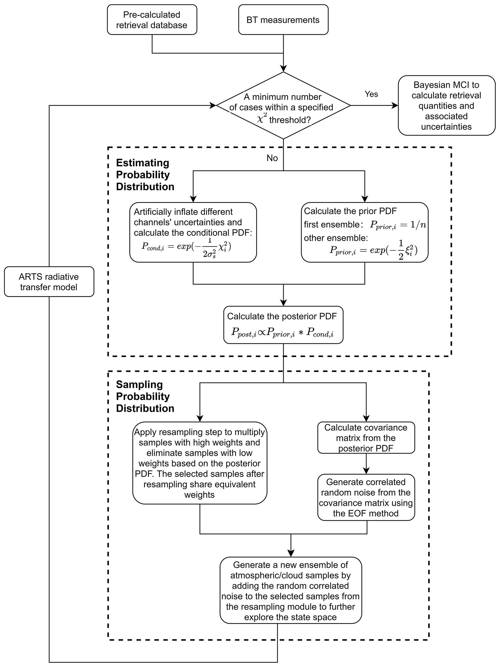
Figure 5Flowchart of the ensemble probability estimation (EnPE) algorithm applied in the radiometer-only retrievals.
We describe the EnPE algorithm in detail here to incorporate improvements in many aspects and to make the algorithm more understandable. The EnPE algorithm stochastically explores the state space by sampling an explicit PDF estimated from promising weighted cases obtained so far from the perspective of Bayesian MCI. As the flowchart in Fig. 5 shows, the algorithm consists of two modules: the PDF estimation module numerically estimates the unknown continuous posterior PDF using the discrete cases with posterior values in the last ensemble, and the PDF sampling module synthesizes new cases according to the accumulated PDF using the resampling approach and the covariance matrix.
Starting from the situation where too few a priori database cases match the observations, the PDF estimation module artificially inflates the measurement uncertainties so that there are enough matches between the observation vector and the BT simulations from the a priori profiles, and the conditional PDF is computed by:
where is the inflation factor ensuring a minimum number of cases in one ensemble are within a specified χ2 threshold. The estimation module then computes the prior PDF to carry along prior information during the iteration to avoid overfitting. The prior PDF is neglected in the first iteration since it is implicitly described by the distribution of the retrieval database cases. We update the prior PDF calculation method in this study to use more accurate prior statistics, and this new approach is discussed later in this subsection. After computing the conditional PDF and the prior PDF, the atmospheric/cloud samples in each ensemble are weighted according to the posterior PDF:
Following this step, the PDF sampling module reselects the samples according to their posterior value to multiply cases with high weights and eliminate cases with low weights. The weights of the selected state vectors become equivalent again. The sampling module then generates correlated random noise using the two-point correlation statistics in the covariance matrix. The covariance matrix of the retrieved quantities is computed using the posterior PDF based on Bayesian MCI:
Liu et al. (2018) conducted the correlated noise generation step by sampling a set of Gaussian distributions in the eigenspace, but a simpler approach is to use the concept of the covariance matrix decomposition. This step is essentially consistent with the Cholesky decomposition applied in the synergistic retrieval in Sect. 3.2.1. However, since the covariance matrix here is not always positive definite, we use the empirical orthogonal functions (EOFs) to generate correlated random variables. The eigenvalues and eigenvectors of the covariance matrix in Eq. (7) are calculated, and the EOFs including 99.9 % of the variance are used. The correlated Gaussian distributed elements are calculated by multiplying the standard Gaussian deviates by the square root of the eigenvalue matrix to scale the data based on the variance magnitude, and then multiplying them by the eigenvector matrix to rotate back to the original axes:
where Σ is the random correlated variables, D is the standard Gaussian derivatives, is the diagonal scaling matrix composed of the square root of eigenvalues, and E is the rotation matrix composed of eigenvectors in each column. Finally, the PDF sampling module builds a new ensemble by adding the correlated random variables to the selected state vectors from the resampling step to further explore the state space.
Once a new ensemble is synthesized and the corresponding BT simulations are computed, the algorithm evaluates the new state samples based on the prior PDF and conditional PDF, and the optimization cycle starts again. As the iteration proceeds, the ensemble evolves and gradually becomes concentrated in the most likely area, compensating for the sparse distribution of the original retrieval database. The cases in the last ensemble are used to calculate the mean parameter values (retrieved values) and standard deviations (retrieved uncertainties) by Bayesian MCI. The EnPE iteration stops when a required number of cases (25 in this study) within the χ2 threshold are found in one ensemble, or the number of iterations is over a limit. If there are not enough cases satisfying the χ2 criterion in the case ensemble, we again inflate the BT measurement standard deviations until covering enough cases. In the retrievals below, the EnPE algorithm generates 300 new cases in each iteration, and only a maximum of two iterations are permitted due to the computation limitation.
We upgrade the precalculated retrieval database with the random cases distributed according to the a priori PDF. In Liu et al. (2018), the prior database is built by relying only on the numerical Global Environmental Multiscale (GEM) (Côté et al., 1998) model outputs. The disadvantages of this method are twofold. First, the random cases cannot well represent the ice cloud distributions because there are many microphysical simplifications in such a numerical model that result in much less microphysical variability than exists in nature. Second, the reference cloud scenes come from the same GEM model, and the interference attributable to the close relations between these two datasets becomes inevitable since the datasets share the same GEM simulation parameters and initial conditions. In this study, we build the retrieval database using the in situ microphysical data and spaceborne radar observations. The remote sensing data are combined with the in situ microphysical PDF using the Bayesian MCI algorithm to create vertical profiles of ice cloud microphysics. After that, the cumulative distribution functions (CDFs) and EOF procedures are applied to capture the single-point and two-point statistics and to create a required number of synthetic microphysical and thermodynamic profiles that are statistically consistent with the Bayesian retrieval results. A comprehensive discussion on creating synthetic ice cloud profiles can be found in Liu and Mace (2020). Consequently, the random cases in the updated retrieval database represent our prior knowledge of the atmospheric and cirrus clouds better, and they are also completely independent of the reference cloud scenes for testing purposes. Further, since the random ice cloud profiles are generated by statistically generalizing a relatively small number of cloud profiles that represent the prior information, a new method is applied to deal with the regularization term (Pprior in Eq. 6) constraining the synthesized profiles to follow the prior knowledge. Compared to the method in Liu et al. (2018), this new approach captures more accurate a priori statistics, and it is applicable even when the a priori PDF is highly non-Gaussian.
The method to calculate the prior PDF is consistent with the control vector transformation concept applied by Evans et al. (2012). The CDFs are used to capture the one-point statistics of the Bayesian retrievals that combine the remote sensing data and in situ microphysics by sorting different ice cloud parameters at different layers from smallest to largest in value and calculating the sum of the assigned equal probabilities up to each datum. The original ice cloud parameters are then represented by their percentile ranks, and the correlations are also preserved in the rank matrix. Following that, the percentile rank matrix is transformed into a Gaussian derivate matrix using the standard normal cumulative distribution function:
where Φ(ξi) is the standard normal cumulative distribution function, and R(xi) is the percentile ranks for different parameters at different layers. For a new ensemble, the ice cloud profiles are transferred into Gaussian derivative matrices to calculate the ξ values, and the associated a priori PDF quantitating the strength of the prior constraints are directly determined by the Gaussian derivatives ξ:
In this way, more realistic ice cloud statistics in arbitrary functional forms are added to the EnPE algorithm as regularizations to make the algorithm more applicable.
3.3 Measurement space and state space
We conduct simulation experiments to assess the synergistic radar and radiometer capability in retrieving ice cloud parameters. The measurement space in the retrieval experiments consists of the noisy radar reflectivity simulations at vertical grid points and the noisy BT simulations of different radiometer channels. Independent Gaussian noise with 1.5 dBz standard deviation characterizing the radar measurement accuracy is added to the simulated radar reflectivity observations, and 4 dBz reflectivity uncertainty that accounts for estimations of the forward model uncertainty due to unknown ice hydrometeor bulk density is assumed during the radar retrieval process. The 4 dBz error estimation is based on the study of Mace and Benson (2017). The grid points with the radar reflectivity below the minimum detectable sensitivity (−25 dBz) are ignored in the retrieval. We add independent Gaussian noise with standard deviation listed in Table 1 to the simulated BT observations, and we use the same noise characteristics in the radiometer retrievals.
The state space in all three retrievals consists of the IWC and NC profiles using the same vertical grids as the reference cloud scenes. The vertical resolution is 250 m. Other atmospheric parameters such as water vapor, temperature, and pressure profiles are set to the true values during the retrieval. For the radar-only and synergistic retrievals, the ice cloud parameters are transformed into lognormal distributions, which means the state variables are ln(IWC) and ln(NC). For the radiometer-only retrievals, the state variables are IWC and NC because we test that the EnPE algorithm works better in non-log scales.
The key element in implementing the Bayesian MCI is to build the retrieval database, which generally consists of two steps: creating random atmosphere and ice cloud properties that are distributed according to the prior PDF and computing the simulated radar reflectivity or BT using the forward model. In this study, we separately develop two retrieval databases for radar and radiometer retrievals using the a priori statistics from TC4 in situ measurements and CloudSat CPR observations.
4.1 Radar retrieval database
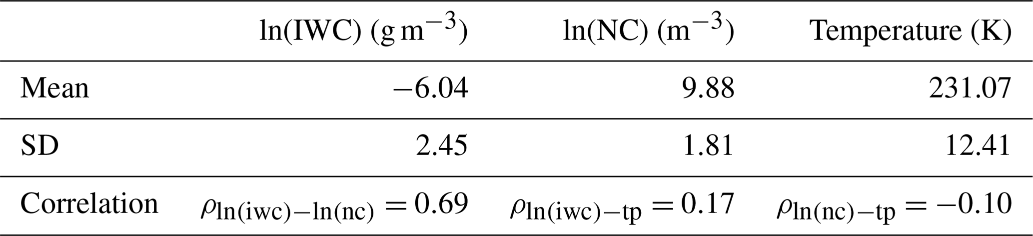
The realistic ice cloud microphysical probability distributions used for building the radar retrieval database is obtained from the in situ data from instruments flown in the TC4 campaign. The in situ ice PSD are obtained from the two-dimensional stereo (2D-S) probe and the precipitation imaging probe (PIP), and the associated temperature is measured by the Meteorological Measurement System on the DC8 aircraft platform. The bimodal PSD scheme which approximates both small and large particle distribution modes by gamma functions is used to fit the in situ data, and the ice cloud parameters, including IWC, NC, and particle size, are derived. More details on the TC4 in situ analysis can be found in Liu and Mace (2020). A multi-variant Gaussian distribution in temperature, ln(IWC), and ln(NC) is used to capture the in situ statistics, using the prior idea that the microphysical parameters are approximately lognormally distributed. Using a multi-variant Gaussian function shows several advantages in generalizing the in situ statistics: First, it specifies the microphysical PDF using a few parameters; second, it facilitates the radar OEM algorithm, which explicitly requires a normally distributed prior PDF; third, it reasonably covers the space where the in situ probes fail to detect, which is important since the random cases need to completely cover the possible parameter range. The parameters for the TC4 multi-variant Gaussian function are summarized in Table 2. An ensemble of random cases (30 000 cases in this study) is sampled from the Gaussian function, and the ARTS radar forward model is used to simulate the reflectivity for each random case.
Table 2Ice particle microphysical statistics defining the a priori Gaussian probability distribution derived from the TC4 in situ data.
The radar retrieval database is used to generate the initial state vector for the radar-only OEM retrieval algorithm based on the Bayesian MCI. This step helps the OEM algorithm to better satisfy the fundamental requirement for a moderately nonlinear forward model. The initial state vector generation step proceeds from top down, and the generated radar attenuation is used to correct the radar reflectivity below. The a priori Gaussian PDF listed in Table 2 is also used in the OEM algorithm as the regularization. We should note that the a priori Gaussian PDF contains single-layer constraints, but it does not describe the vertical correlations between ice cloud microphysics at different layers.
Figure 6 shows the two-dimensional histogram for the microphysical quantities and reflectivity simulations in the radar retrieval database. A fairly strong correlation between IWC and NC over the whole range is observed in the left panel. The middle panel and the right panel indicate that the radar reflectivity simulations have a strong correlation with IWC in the whole range, but its correlation with NC is much weaker.
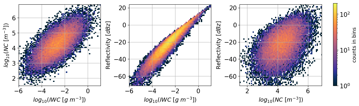
Figure 6Two-dimensional histogram for the microphysical quantities and the W-band radar reflectivity simulations derived from the random cases in the precalculated radar retrieval database.
4.2 Radiometer retrieval database
Apart from using the TC4 in situ microphysical statistics, we also use the CloudSat observations to acquire the critical coherent vertical correlations to synthesize the random ice cloud profiles for creating the radiometer retrieval database. The data we use include CloudSat radar reflectivity, CALIPSO lidar cloud fraction, and the corresponding ECMWF profiles of temperature and relative humidity. As mentioned in Sect. 3.2.2, the active remote sensing profiles are first combined with the TC4 cloud microphysical probability distributions using the Bayesian MCI algorithm, and then the CDFs/EOFs procedures are applied to create a required number of synthetic microphysical and thermodynamic profiles (100 000 profiles in this study) using the one-point and two-point statistics that are captured from the Bayesian retrieval results. More details can be found in Liu and Mace (2020).
Figure 7 shows the profiles of IWC, NC, temperature, and relative humidity for seven percentiles in the cumulative distributions. Layers that are identified as clear are added with random Gaussian noise to prevent discontinuity in the CDFs. The mean values for the added IWC and NC noise are 10−6 g m−3 and 10 m−3, respectively. The left two panels show that the a priori IWC profiles cover the range from clear condition to about 10 g m−3, and the NC profiles cover the range up to about 106 m−3. The 75 % curve implies that a large majority of atmospheric conditions are outside the 9–14 km range. The right two panels show that the a priori temperature profiles have a small range of temperature coverage under the tropical atmospheric conditions applied in this study, and the relative humidity profiles have a large possible range, almost coving the entire possible values from 0 to 1.
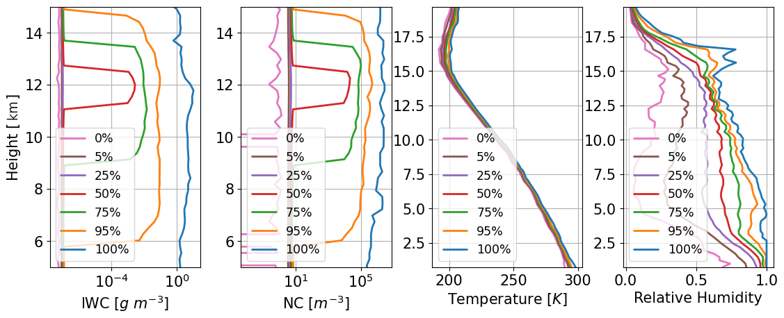
Figure 7Profiles of ice water content (IWC), number concentration (NC), temperature, and relative humidity for seven percentiles in the cumulative distributions for the random atmospheric/cloud profiles in the precalculated radiometer retrieval database.
The precalculated retrieval database provides a good opportunity for estimating the degrees of freedom (DoF) for the ACCP (sub)millimeter-wave radiometer. The DoF describes the number of independent pieces of information in the radiometer measurement since some channels provide redundant information. The DoF is usually calculated as the trace of the averaging kernel matrix based on the Jacobian matrix (Rodgers, 2000), but a more general method described in Eriksson et al. (2020) is employed since the Jacobian matrix for BT is not estimated here. This method calculates the DoF in the measurement space based on the EOF approach. The covariance matrix of a set of simulated BT is decomposed using EOF:
where E is the matrix with eigenvectors in each column, and Λ is the diagonal matrix containing the corresponding eigenvalues. The Gaussian measurement noise in eigenspace is transformed back using the same eigen coordinate axes:
where Sε is the diagonal matrix that contains the square of measurement noise for different channels. The DoF is defined as the number of diagonal elements in Sy that are larger than the corresponding value in SΛ in the same place.
Figure 8 shows the DoF of the ACCP radiometer as the function of the IWP and integrated water vapor (IWV) using the measurement noise characteristics listed in Table 1. The DoF is computed only when the number of random cases in a certain IWV–IWP bin is larger than 10 to avoid noise interference. It can be seen that the DoF increases with IWP, but it decreases as the IWV becomes large. For the wet atmospheres with IWV larger than 42 kg m−2, the DoF is generally smaller than 6 when IWP is below 100 g m−2, and it is between 7 and 9 in the 100–500 g m−2 IWP range. The DoF reaches 12 as the IWP goes beyond 500 g m−2. For the dry atmospheres with IWV smaller than 42 kg m−2, the DoF is high even at low IWP conditions, generally between 6 and 11 when IWP is smaller than 100 g m−2, and the DoF is mostly 12 when the IWP is over 100 g m−2. We should note that the DoFs here are estimated based on the atmospheric profiles that only contain ice cloud hydrometer species. The DoF estimations using more sophisticated atmospheric and cloud conditions that include multiply types of hydrometer are likely to be different.
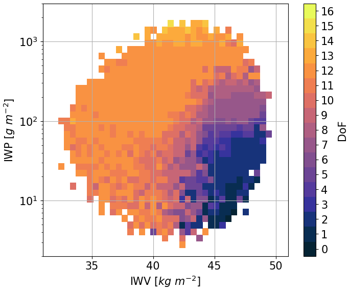
Figure 8The degrees of freedom (DoF) for the ACCP radiometer candidate as a function of the ice water path (IWP) and integrated water vapor (IWV). The DoF is estimated using the radiometer retrieval database that has 100 000 random ice cloud profiles. Liquid hydrometer species are not included in the retrieval database.
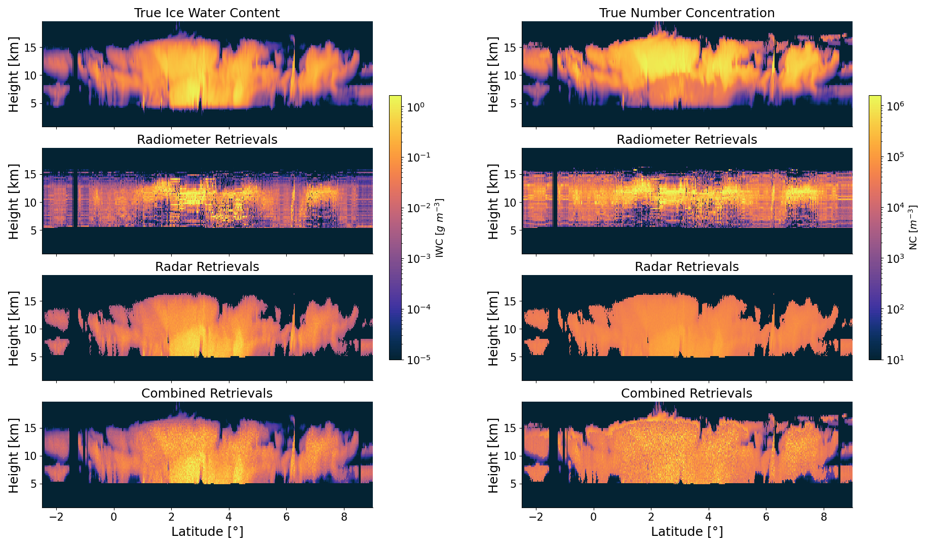
Figure 9Comparison between the true values and the retrieval results for ice water content and number concentration profiles along the selected latitude transect. The results for radar-only, radiometer-only, and combined retrievals are presented sequentially.
In this section we present the analytical results for the radiometer-only, radar-only, and synergistic retrievals to assess the capability of the objective ACCP remote sensors in retrieving ice cloud parameters. The retrieval experiments are performed by inputting the simulated noisy radar reflectivity and BT observations into the hybrid Bayesian algorithms and then comparing the retrieved parameters with the true values to determine the retrieval accuracy.
Figure 9 shows a side-by-side comparison between the true values and the retrieval results for IWC and NC profiles along the ECCC model transect. The results for the radar-only, radiometer-only, and combined retrievals are presented sequentially. The passive-only retrieval results suggest that there is very little if any information regarding the vertical distribution of ice cloud microphysics in the radiometer measurements when considered without the radar measurements. For the active-only retrievals, the retrieved IWC profiles realistically reproduce the vertical structure of the reference cloud scenes. The retrieved values also correspond to the true values in general, even though sometimes the retrievals tend to underestimate the IWC values, especially near the top of the cloud ranging from 10 to 15 km in height. By contrast, the active-only retrievals for NC profiles perform much worse. The true NC values cover the range from 10 to over 106 m−3, but the radar retrievals do not match this variability, usually concentrating in the 103–105 m−3 range. The retrieval results again illustrate that the radar measurements are much more sensitive to the IWC variation compared to the NC variation. For the synergistic retrievals, obvious perturbations can be observed for both IWC and NC profiles and the results become less smooth compared to the radar-only retrievals. The added radiometer observations tend to correct the IWC underestimation discussed above by constraining the vertically integrated condensed mass.
Figure 10 shows the retrieved IWP values for the passive-only, active-only, and combined retrievals based on the hybrid Bayesian algorithms along the latitudinal transect. For the passive-only retrievals, the retrieval errors are comparable to the active-involved retrievals over the entire range. The active-only retrievals show the tendency to overestimate the IWP for thin clouds but underestimate the thick cloud IWP. The combined retrievals are based on the radar OEM results, and substantial improvements in IWP retrieval accuracy can be seen after adding the ACCP BT measurements.
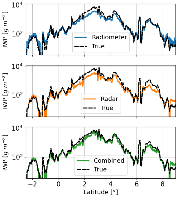
Figure 10Direct comparison between the retrieved ice water path (IWP) and the true values along the latitudinal transect. The passive-only, radar-only, and combined retrievals are all displayed.
Figure 11 shows the scatterplots of the retrieved parameters against the true values that are colored by density to further visualize the retrieval performance. The statistical IWC analysis below only applies to the grid points with the reference IWC larger than 10−5 g m−3. Similarly, the bottom limitations for NC and IWP analysis are 100 m−3 and 10 g m−2, respectively. The scatterplots for IWC, NC, and IWP are shown in different columns, and the plots for passive-only, active-only, and combined retrievals are shown in different rows. This figure can be directly compared with Figs. 7, 8, and 13 in Pfreundschuh et al. (2020), and a similar phenomenon can be observed here. Starting from the IWC retrievals in the first column, the passive-only retrievals show the largest deviations from the diagonal line, which is not surprising since the BT measurements have low sensitivity to the vertical distribution of the ice cloud microphysics. The radar-only retrievals provide much more accurate results. The scatter of points lies along the diagonal and the associated deviations are small. The radar-only retrievals are observed to bias high for the tenuous clouds and bias low when IWC values are high. The prior constraint is possibly the reason for causing both low-end and high-end biases since the particles with extreme values possess small prior probability values. Another possibility is that we do not differentiate the cloud ice and snow in the forward model. The combined retrievals correct the high-end offset, and the scatter plots lie more along the diagonal. The rim of the scatter plots becomes less smooth, which is inevitable because the BT measurements are added through an ensemble approach by generating random cases over a large possible range to statistically explore the state space. However, its systematic deviations are reduced compared to the radar-only retrievals, which is consistent with the analysis in Pfreundschuh et al. (2020). It is also seen that the retrieval accuracies when IWC is larger than 10−2 g m−3 are improved after adding BT observations. The combined retrievals, together with the radiometer-only retrievals shown in the top panel, suggest that the radiometer measurements possess high sensitivity for large particles with IWC over 10−2 g m−3. For the NC retrievals in the second column, the passive-only retrievals again show very little capability. The NC results from the radar-only retrievals do not follow the true values well. The retrieved values are always located in the range of 104–105 m−3 although the true values vary in a much wider range. The combined retrievals improve the NC accuracies only when NC is over 104 m−3, but the overall performance is still poor. Again, the combined retrievals and radiometer-only retrievals together suggest that the radiometer measurements are sensitive for particles with NC larger than 10−4 m−3. The IWP retrievals show very good performance overall. All retrieved values in different panels follow the true values with small associated deviations. The IWP results from passive-only retrievals tend to overestimate the true values when IWP is small and underestimate the true values when IWP is large. The underestimation performance could probably be corrected if more random atmospheric/cloud profiles covering the large IWP range are included in the precalculated radiometer retrieval database. The active-only retrievals show a similar tendency, and significant improvements could be seen for the results from the combined retrievals.
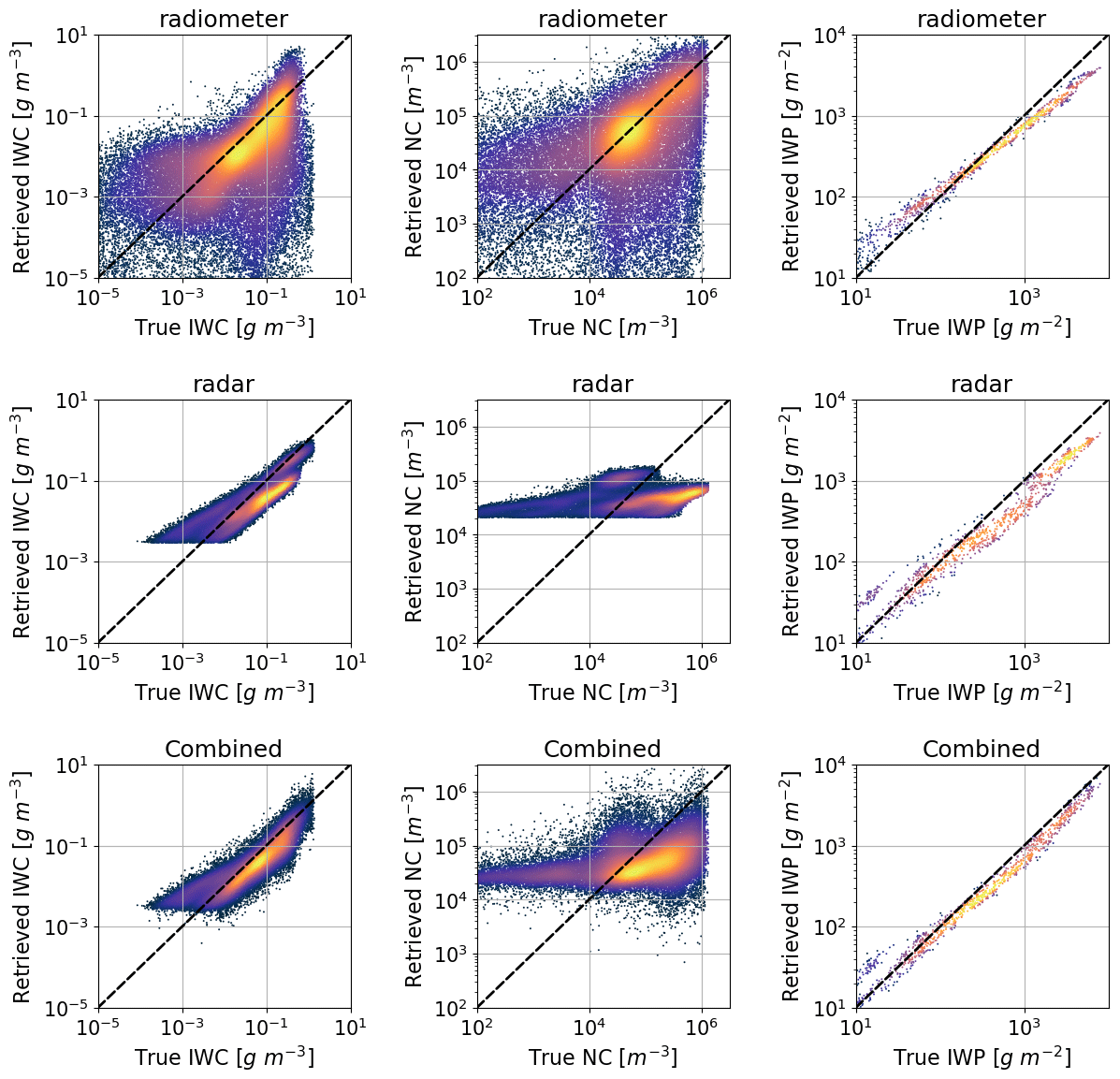
Figure 11The scatterplots of the retrieved parameters against the true values that are colored by density. The scatterplots for ice water content (IWC), number concentration (NC), and ice water path (IWP) are shown in different columns, and the plots for passive-only, active-only, and combined retrievals are shown in different rows.
Figure 12 displays the PDF of the logarithmic errors for different parameters under different retrieval methods. The logarithmic error is defined as:
The negative/positive values of Elog 10 indicate that the retrieved values are smaller/larger than the true values, and 0 B error shows that the retrieved value and true value are identical; 1 B error is a factor of 10. For the IWC retrievals in the left panel, the radiometer-only retrievals show the strongest deviation with the logarithmic errors spreading from −4 to +2 B. Compared to the radar-only retrievals, the PDF of the synergistic retrievals has a smaller offset and smaller variance, even though the improvements are not substantial. The logarithmic errors of the NC retrievals in the middle panel spread from −2.5 to 2.5 B, indicating poor NC constraints from the radar and radiometer observations. As for the IWP retrieval displayed in the right panel, the passive-only and active-only retrievals show comparable retrieval errors, and significant improvements using the synergistic observations are evident.

Figure 12The probability density function (PDF) of the logarithmic errors for different ice cloud parameters under different retrieval methods.
Figure 13 shows the quantitative values measuring logarithmic error distribution to compare the retrieval accuracy under different retrievals. Panels Fig. 13a and b show the mean values of the logarithmic errors and the associated IQR. The IQR is defined as the difference between the 75th and 25th percentile. The mean and IQR values were also presented in Fig. 11 in Pfreundschuh et al. (2020). However, since substantial differences in underlying assumptions exist in these two studies, the quantitative values presented here could not be directly compared with those in Pfreundschuh et al. (2020). The differences are primarily reflected in the following aspects. The PSD schemes used in these two studies are not identical, and the a priori PDF constraining the optimization is significantly different. Further, as mentioned in Sect. 2.3, we do not investigate the systematic biases coming from various particle habits, which results in much smaller absolute mean and IQR values compared with the results in Pfreundschuh et al. (2020). Nevertheless, the results could still be compared qualitatively to see whether similar tendencies exist. For the IWC retrievals, the radiometer-only retrievals show the largest retrieval errors. Compared to the radar-only retrievals, the combined retrievals correct the systematic biases, but the improvements in decreasing the IQR spreads are not evident. For the NC retrievals, the radar-only and radiometer-only results are both unsatisfactory and their IQR values are similar. For the IWP retrievals, the radiometer-only and radar-only show comparable capabilities, and the improvements from the combined retrievals are obvious since both biases and IQR deviations decrease. The tendencies observed in IWC and IWP retrievals here are generally consistent with the findings in Pfreundschuh et al. (2020). Panel Fig. 13c shows the root mean square deviation (RMSD) for different parameters to measure the deviations against zero. Not surprisingly, the radiometer-only retrievals have the highest number for both IWC and NC. The radar-only retrievals have a small RMSD value for IWC and a large RMSD value for NC, and the combined retrievals decrease the number on this basis. Since the RMSD is easily skewed by a few poor retrievals, the robust median of the absolute logarithmic errors that separate the higher half from the lower half in all the absolute logarithmic errors is displayed in panel d. Overall, 50 % of the retrievals have an error less than the median error, and 50 % have a larger error. The median fractional error is used to quantitatively assess the relative improvements after adding BT measurements into the radar-only retrievals. The median bias for IWC retrievals decreases from 0.34 to 0.28, indicating an 18 % improvement, and the bias for NC decreases from 0.73 to 0.62, indicating a 12 % improvement obtained from the BT information. The biggest improvement exists in IWP retrievals, which decreases the median bias from 0.19 to 0.11, and the relative improvements reach 42 %.
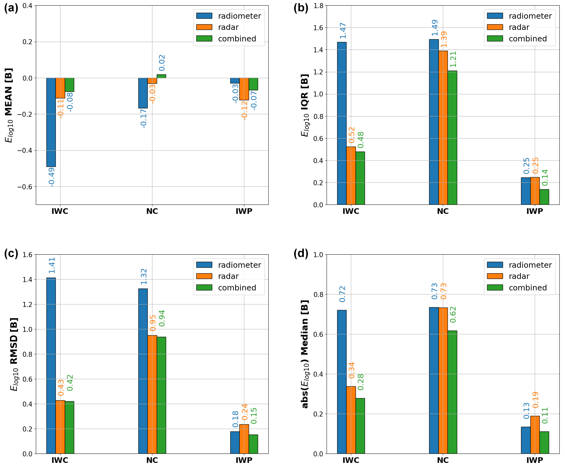
Figure 13The quantitative statistics of the logarithmic errors for the retrieved ice cloud quantities. Panels (a) and (b) show the mean values and the interquartile range (IQR), and (c) shows the root mean square deviation (RMSD) of the logarithmic errors. Panel (d) shows the median values of the absolute logarithmic errors that separate the higher half from the lower half in all the retrieval error estimations.
In this study, we develop a suite of hybrid Bayesian retrieval algorithms to assess a candidate observing system representative of what is being considered for the decadal survey clouds-convection-precipitation designated observable mission to be flown later this decade. We specifically evaluate the capability of an observing system consisting of a W-band radar and a (sub)millimeter-wave radiometer in constraining the ice cloud microphysics. Our purpose is to demonstrate the value of single-instrument and synergistic retrievals of ice cloud microphysical parameters. Several new algorithms are proposed here, which could serve as alternative solutions for exploring the synergistic active and passive retrieval concepts for the actual instruments once they are known. The geophysical variables we investigate include the IWC, NC, and IWP. The hybrid Bayesian algorithms combine the Bayesian MCI and optimization processes to compute retrieval quantities and associated uncertainties. The radar-only retrievals employ the OEM optimization algorithm that uses gradient information to minimize the cost function. The OEM is initialized by a state vector that is constructed by implementing Bayesian MCI to the radar reflectivity at different grid points using the precalculated radar database. The necessary Jacobian matrix is calculated by perturbing the ice cloud microphysical quantities on different layers. The radiometer-involved retrievals employ ensemble strategies to optimize the ill-posted problem. The synergistic radar and radiometer retrievals are done by generating random cases from the radar OEM results based on the Cholesky decomposition technique. The BT simulations are then computed, and the Bayesian MCI is implemented to derive the final retrieval results. For the radiometer-only retrievals, the EnPE algorithm is applied to statistically estimate the posterior PDF using the promising weighted cases. The estimation module and the sampling module proceed iteratively to stochastically explore the state space. In addition, a new approach to implement prior constraints that enable the a priori PDF to be highly non-Gaussian is proposed in order to make the ensemble algorithm more applicable.
We conducted simulation experiments to evaluate the accuracy of retrieving ice cloud quantities for different remote sensors. The simulated noisy radar reflectivity and BT observations are input to the hybrid Bayesian algorithms, and the retrieved parameters are compared with the known values to determine the retrieval accuracies. A tropical transect of cloud profiles that are simulated using the ECCC model is selected as the reference cloud scenes. This choice ensures the independence between the atmospheric/cloud profiles for testing and the vertical profiles in the a priori database. The simulation experiments assume that both sensors have the same nadir-looking viewing angle. The influence of different footprints and viewing geometries between the active and passive remote sensors are neglected in this initial study but will be evaluated once the specific parameters of the observing system are known. Since we do not consider the forward model uncertainties from various particle habits, the retrieval errors are much smaller than the results in Pfreundschuh et al. (2020). Nevertheless, consistent results can still be qualitatively observed here. The main conclusions from the results presented here can be summarized as:
1. The radiometer measurements do not have direct information about the IWC and NC vertical distribution. However, the BT measurements possess high sensitivity for large ice cloud particles with IWC values larger than 10−2 g m−3 and NC values larger than 104 m−3.
2. The radar-only retrieval demonstrates capability in retrieving IWC profiles, but it literally does not exhibit capabilities in retrieving NC vertical distribution. The radar-only retrievals for IWP have comparable accuracies to the radiometer-only retrievals.
3. The synergistic retrievals have evident improvements in retrieval accuracies compared with the radar-only retrievals. When using the median of the absolute fractional error as the quantitative parameter to evaluate the retrieval accuracies, the relative improvements after adding BT measurements for IWC, NC, and IWP are 18 % and 12 %, and 42 %, respectively.
This paper provides an end-to-end idealized simulation experiment that sacrifices precise reality in order to demonstrate nuances in the various algorithms, and several disadvantages are worth mentioning. First, there are many simplifications on the reference cloud scenes and the radiative transfer model. We only use the frozen particles in the reference cloud scenes, and the liquid clouds are ignored. The impacts from water vapor uncertainties are also neglected. Further, only one particle habit is applied and the forward model uncertainties from particle habits and PSD are not considered. These simplifications facilitate the quantitative evaluation of the proposed retrieval algorithms without complication from parameters not yet known so that the relative benefit of the observing system is considered as separate instruments or as a synergistic set. In all cases the value of synergy is demonstrated although more realistic observing systems must be considered in future work. Second, the statistical characteristics are only derived based on selected atmospheric/cloud profiles along a single latitudinal transect. Since this subset with a finite number of profiles can hardly represent the realistic spatial distribution of ice cloud microphysics that will be encountered globally, the statistics we derive may differ from the characteristics of the entire possible atmospheric conditions. Third, apart from the W-band radar and the (sub)millimeter-wave radiometer, the eventual observing system will likely include other remote sensors that would be useful for improving retrieval accuracies for ice cloud remote sensing. For instance, the eventual radar system will likely be dual-frequency and add Ku- or Ka-band to the measurements. Also, highly accurate Doppler velocity measurements will likely be observed that may allow for constraints on the ice crystal bulk density that could significantly mitigate forward model uncertainties. These problems will be investigated in future work.
The retrieval algorithm modules and the codes used to produce the results in this study are available upon request from the corresponding author.
The Environment and Climate Change Canada (ECCC) dataset used as the reference cloud scenes is available upon request from the corresponding author.
YL developed the retrieval algorithms, set up the retrieval experiments, analyzed the retrieval results, and wrote the article. GGM acted as project leader, provided guidance and insight regarding experiment configurations and results analysis.
The contact author has declared that neither they nor their co-authors have any competing interests.
Publisher’s note: Copernicus Publications remains neutral with regard to jurisdictional claims in published maps and institutional affiliations.
We thank for Pavlos Kollias at Stony Brook University for providing the atmospheric scenes from the ECCC model that we used for evaluating the synergistic retrievals. The TC4 in situ data for this study were collected by the members of the Stratton Park Engineering Corporation led by Paul Lawson, as well as Andrew Heymsfield at the National Center for Atmospheric Research. The CloudSat data were obtained from the CloudSat Data Processing Center at the Colorado State University’s Cooperative Institute for Research in the Atmosphere (CIRA). All TC4 data are publicly and freely available in the NASA data archive at https://espoarchive.nasa.gov/archive/browse/tc4 (last access: 18 February 2022), and the CloudSat data are available at http://www.cloudsat.cira.colostate.edu/data-products (last access: 18 February 2022).
This research has been supported by the Goddard Space Flight Center (NASA ACE and ACCP programs (grant nos. NNX15AK17G and 80NSSC19K1087)).
This paper was edited by Patrick Eriksson and reviewed by two anonymous referees.
Ackerman, T. P., Liou, K.-N., Valero, F. P., and Pfister, L.: Heating rates in tropical anvils, J. Atmos. Sci., 45, 1606–1623, https://doi.org/10.1175/1520-0469(1988)045<1606:HRITA>2.0.CO;2, 1988. a
Berry, E. and Mace, G. G.: Cloud properties and radiative effects of the Asian summer monsoon derived from A-Train data, J. Geophys. Res.-Atmos., 119, 9492–9508, https://doi.org/10.1002/2014JD021458, 2014. a
Brath, M., Fox, S., Eriksson, P., Harlow, R. C., Burgdorf, M., and Buehler, S. A.: Retrieval of an ice water path over the ocean from ISMAR and MARSS millimeter and submillimeter brightness temperatures, Atmos. Meas. Tech., 11, 611–632, https://doi.org/10.5194/amt-11-611-2018, 2018. a
Buehler, S. A., Defer, E., Evans, F., Eliasson, S., Mendrok, J., Eriksson, P., Lee, C., Jiménez, C., Prigent, C., Crewell, S., Kasai, Y., Bennartz, R., and Gasiewski, A. J.: Observing ice clouds in the submillimeter spectral range: the CloudIce mission proposal for ESA's Earth Explorer 8, Atmos. Meas. Tech., 5, 1529–1549, https://doi.org/10.5194/amt-5-1529-2012, 2012. a
Buehler, S. A., Mendrok, J., Eriksson, P., Perrin, A., Larsson, R., and Lemke, O.: ARTS, the Atmospheric Radiative Transfer Simulator – version 2.2, the planetary toolbox edition, Geosci. Model Dev., 11, 1537–1556, https://doi.org/10.5194/gmd-11-1537-2018, 2018. a
Chen, J., Pendlebury, D., Gravel, S., Stroud, C., Ivanova, I., DeGranpré, J., and Plummer, D.: Development and Current Status of the GEM-MACH-Global Modelling System at the Environment and Climate Change Canada, in: Air Pollution Modeling and its Application XXVI, edited by: Mensink, C., Gong, W., and Hakami, A., ITM 2018, Springer Proceedings in Complexity, Springer, Cham, 107–112,https://doi.org/10.1007/978-3-030-22055-6_18, 2020. a
Côté, J., Gravel, S., Méthot, A., Patoine, A., Roch, M., and Staniforth, A.: The operational CMC–MRB global environmental multiscale (GEM) model. Part I: Design considerations and formulation, Mon. Weather Rev., 126, 1373–1395, https://doi.org/10.1175/1520-0493(1998)126<1373:TOCMGE>2.0.CO;2, 1998. a
Delanoë, J., Protat, A., Testud, J., Bouniol, D., Heymsfield, A., Bansemer, A., Brown, P., and Forbes, R.: Statistical properties of the normalized ice particle size distribution, J. Geophys. Res.-Atmos., 110, D10, https://doi.org/10.1029/2004JD005405, 2005. a
Eriksson, P., Ekelund, R., Mendrok, J., Brath, M., Lemke, O., and Buehler, S. A.: A general database of hydrometeor single scattering properties at microwave and sub-millimetre wavelengths, Earth Syst. Sci. Data, 10, 1301–1326, https://doi.org/10.5194/essd-10-1301-2018, 2018. a
Eriksson, P., Rydberg, B., Mattioli, V., Thoss, A., Accadia, C., Klein, U., and Buehler, S. A.: Towards an operational Ice Cloud Imager (ICI) retrieval product, Atmos. Meas. Tech., 13, 53–71, https://doi.org/10.5194/amt-13-53-2020, 2020. a
Evans, K. F.: SHDOMPPDA: A radiative transfer model for cloudy sky data assimilation, J. Atmos. Sci., 64, 3854–3864, https://doi.org/10.1175/2006JAS2047.1, 2007. a
Evans, K. F., Walter, S. J., Heymsfield, A. J., and McFarquhar, G. M.: Submillimeter-wave cloud ice radiometer: Simulations of retrieval algorithm performance, J. Geophys. Res.-Atmos., 107, AAC 2-1–AAC 2-21, https://doi.org/10.1029/2001JD000709, 2002. a, b, c
Evans, K. F., Wang, J. R., Racette, P. E., Heymsfield, G., and Li, L.: Ice cloud retrievals and analysis with the compact scanning submillimeter imaging radiometer and the cloud radar system during CRYSTAL FACE, J. Appl. Meteorol., 44, 839–859, https://doi.org/10.1175/JAM2250.1, 2005. a, b, c
Evans, K. F., Wang, J. R., O'C Starr, D., Heymsfield, G., Li, L., Tian, L., Lawson, R. P., Heymsfield, A. J., and Bansemer, A.: Ice hydrometeor profile retrieval algorithm for high-frequency microwave radiometers: application to the CoSSIR instrument during TC4, Atmos. Meas. Tech., 5, 2277–2306, https://doi.org/10.5194/amt-5-2277-2012, 2012. a, b, c
Hartmann, D. L. and Berry, S. E.: The balanced radiative effect of tropical anvil clouds, J. Geophys. Res.-Atmos., 122, 5003–5020, https://doi.org/10.1002/2017JD026460, 2017. a
Illingworth, A. J., Barker, H., Beljaars, A., Ceccaldi, M., Chepfer, H., Clerbaux, N., Cole, J., Delanoë, J., Domenech, C., Donovan, D. P., et al.: The EarthCARE satellite: The next step forward in global measurements of clouds, aerosols, precipitation, and radiation, B. Am. Meteorol. Soc., 96, 1311–1332, https://doi.org/10.1175/BAMS-D-12-00227.1, 2015. a
Jiménez, C., Buehler, S., Rydberg, B., Eriksson, P., and Evans, K.: Performance simulations for a submillimetre-wave satellite instrument to measure cloud ice, Q. J. Roy. Meteor. Soc., 133, 129–149, https://doi.org/10.1002/qj.134, 2007. a
Kangas, V., D'Addio, S., Klein, U., Loiselet, M., Mason, G., Orlhac, J.-C., Gonzalez, R., Bergada, M., Brandt, M., and Thomas, B.: Ice cloud imager instrument for MetOp Second Generation, in: 13th Specialist Meeting on Microwave Radiometry and Remote Sensing of the Environment (MicroRad), Pasadena, CA, USA, 18 August 2014, 228–231, https://doi.org/10.1109/MicroRad.2014.6878946, 2014. a
Liou, K.-N.: Influence of cirrus clouds on weather and climate processes: A global perspective, Mon. Weather Rev., 114, 1167–1199, https://doi.org/10.1175/1520-0493(1986)114<1167:IOCCOW>2.0.CO;2, 1986. a
Liu, Y. and Mace, G. G.: Synthesizing the Vertical Structure of Tropical Cirrus by Combining CloudSat Radar Reflectivity With In Situ Microphysical Measurements Using Bayesian Monte Carlo Integration, J. Geophys. Res.-Atmos., 125, e2019JD031882, https://doi.org/10.1029/2019JD031882, 2020. a, b, c
Liu, Y., Buehler, S. A., Brath, M., Liu, H., and Dong, X.: Ensemble Optimization Retrieval Algorithm of Hydrometeor Profiles for the Ice Cloud Imager Submillimeter-Wave Radiometer, J. Geophys. Res.-Atmos., 123, 4594–4612, https://doi.org/10.1002/2017JD027892, 2018. a, b, c, d, e
Mace, G. and Benson, S.: Diagnosing cloud microphysical process information from remote sensing measurements – A feasibility study using aircraft data. Part I: Tropical anvils measured during TC4, J. Appl. Meteorol. Clim., 56, 633–649, https://doi.org/10.1175/JAMC-D-16-0083.1, 2017. a
McFarlane, S. A., Evans, K. F., and Ackerman, A. S.: A Bayesian algorithm for the retrieval of liquid water cloud properties from microwave radiometer and millimeter radar data, J. Geophys. Res.-Atmos., 107, AAC 12-1–AAC 12-21, https://doi.org/10.1029/2001JD001011, 2002. a, b
National Academies of Sciences, Engineering, and Medicine: Thriving on our changing planet: A decadal strategy for Earth observation from space, The National Academies Press, Washington, DC, https://doi.org/10.17226/24938, 2018. a
Petty, G. W. and Huang, W.: The modified gamma size distribution applied to inhomogeneous and nonspherical particles: Key relationships and conversions, J. Atmos. Sci., 68, 1460–1473, https://doi.org/10.1175/2011JAS3645.1, 2011. a
Pfreundschuh, S., Eriksson, P., Buehler, S. A., Brath, M., Duncan, D., Larsson, R., and Ekelund, R.: Synergistic radar and radiometer retrievals of ice hydrometeors, Atmos. Meas. Tech., 13, 4219–4245, https://doi.org/10.5194/amt-13-4219-2020, 2020. a, b, c, d, e, f, g, h, i, j
Prigent, C., Aires, F., Wang, D., Fox, S., and Harlow, C.: Sea-surface emissivity parametrization from microwaves to millimetre waves, Q. J. Roy. Meteor. Soc., 143, 596–605, https://doi.org/10.1002/qj.2953, 2017. a
Rodgers, C. D.: Inverse methods for atmospheric sounding: theory and practice, World scientific, 2, https://doi.org/10.1142/3171, 2000. a, b, c, d
Rothman, L. S., Gordon, I. E., Babikov, Y., Barbe, A., Benner, D. C., Bernath, P. F., Birk, M., Bizzocchi, L., Boudon, V., Brown, L. R., et al.: The HITRAN2012 molecular spectroscopic database, J. Quant. Spectrosc. Ra., 130, 4–50, https://doi.org/10.1016/j.jqsrt.2013.07.002, 2013. a
Stamnes, K., Tsay, S.-C., Wiscombe, W., and Laszlo, I.: DISORT, a general-purpose Fortran program for discrete-ordinate-method radiative transfer in scattering and emitting layered media: documentation of methodology, 2000. a
Stephens, G. L., Vane, D. G., Tanelli, S., Im, E., Durden, S., Rokey, M., Reinke, D., Partain, P., Mace, G. G., Austin, R., et al.: CloudSat mission: Performance and early science after the first year of operation, J. Geophys. Res.-Atmos., 113, D8, https://doi.org/10.1029/2008JD009982, 2008. a
Toon, O. B., Starr, D. O., Jensen, E. J., Newman, P. A., Platnick, S., Schoeberl, M. R., Wennberg, P. O., Wofsy, S. C., Kurylo, M. J., Maring, H., et al.: Planning, implementation, and first results of the Tropical Composition, Cloud and Climate Coupling Experiment (TC4), J. Geophys. Res.-Atmos., 115, D10, https://doi.org/10.1029/2009JD013073, 2010. a
Zelinka, M. D. and Hartmann, D. L.: The observed sensitivity of high clouds to mean surface temperature anomalies in the tropics, J. Geophys. Res.-Atmos., 116, D23, https://doi.org/10.1029/2011JD016459, 2011. a