Air temperature equation derived from sonic temperature and water vapor mixing ratio for turbulent airflow sampled through closed-path eddy-covariance flux systems

Air temperature (T) plays a fundamental role in many aspects of the flux exchanges between the atmosphere and ecosystems. Additionally, knowing where (in relation to other essential measurements) and at what frequency T must be measured is critical to accurately describing such exchanges. In closed-path eddy-covariance (CPEC) flux systems, T can be computed from the sonic temperature (T_s) and water vapor mixing ratio that are measured by the fast-response sensors of a three-dimensional sonic anemometer and infrared CO₂–H₂O analyzer, respectively. T is then computed by use of either $T=T_{\mathrm{s}}{\left(\mathrm{1}+\mathrm{0.51}q\right)}^{-\mathrm{1}}$, where q is specific humidity, or $T=T_{\mathrm{s}}{\left(\mathrm{1}+\mathrm{0.32}e/P\right)}^{-\mathrm{1}}$, where e is water vapor pressure and P is atmospheric pressure. Converting q and $e/P$ into the same water vapor mixing ratio analytically reveals the difference between these two equations. This difference in a CPEC system could reach ±0.18 K, bringing an uncertainty into the accuracy of T from both equations and raising the question of which equation is better. To clarify the uncertainty and to answer this question, the derivation of T equations in terms of T_s and H₂O-related variables is thoroughly studied. The two equations above were developed with approximations; therefore, neither of their accuracies was evaluated, nor was the question answered. Based on first principles, this study derives the T equation in terms of T_s and the water vapor molar mixing ratio (${\mathit{\chi }}_{{\mathrm{H}}_{\mathrm{2}}\mathrm{O}}$) without any assumption and approximation. Thus, this equation inherently lacks error, and the accuracy in T from this equation (equation-computed T) depends solely on the measurement accuracies of T_s and ${\mathit{\chi }}_{{\mathrm{H}}_{\mathrm{2}}\mathrm{O}}$. Based on current specifications for T_s and ${\mathit{\chi }}_{{\mathrm{H}}_{\mathrm{2}}\mathrm{O}}$ in the CPEC300 series, and given their maximized measurement uncertainties, the accuracy in equation-computed T is specified within ±1.01 K. This accuracy uncertainty is propagated mainly (±1.00 K) from the uncertainty in T_s measurements and a little (±0.02 K) from the uncertainty in ${\mathit{\chi }}_{{\mathrm{H}}_{\mathrm{2}}\mathrm{O}}$ measurements. An improvement in measurement technologies, particularly for T_s, would be a key to narrowing this accuracy range. Under normal sensor and weather conditions, the specified accuracy range is overestimated, and actual accuracy is better. Equation-computed T has a frequency response equivalent to high-frequency T_s and is insensitive to solar contamination during measurements. Synchronized at a temporal scale of the measurement frequency and matched at a spatial scale of measurement volume with all aerodynamic and thermodynamic variables, this T has advanced merits in boundary-layer meteorology and applied meteorology.

1 Introduction

The equation of state, P=ρRT, is a fundamental equation for describing all atmospheric flows, where P is atmospheric pressure, ρ is moist-air density, R is the gas constant for moist air, and T is air temperature (Wallace and Hobbs, 2006). In boundary-layer flow, where turbulence is nearly always present, accurate representation of the “state” of the atmosphere at any given “point” and time requires consistent representation of spatial and temporal scales for all thermodynamic factors of P, ρ, and T (Panofsky and Dutton, 1984). Additionally, for observing fluxes describing exchanges of quantities, such as heat and moisture between the Earth and the atmosphere, it is critical to know all three-dimensional (3-D) components of wind speed at the same location and temporal scale as the thermodynamic variables (Laubach and McNaughton, 1998).

In a closed-path eddy-covariance (CPEC) system, the 3-D wind components and sonic temperature (T_s) are measured by a 3-D sonic anemometer in the sonic measurement volume near which air is sampled through the orifice of an infrared H₂O–CO₂ analyzer (hereafter referred to as the infrared analyzer) into its closed-path H₂O–CO₂ measurement cuvette, where air moisture is measured by the analyzer (Fig. 1). The flow pressure inside the cuvette (P_c) and the differential (ΔP) between P_c and ambient flow pressure in the sampling location are also measured (Campbell Scientific Inc., 2018c). Atmospheric P in the sampling volume, therefore, is a sum of P_c and ΔP. P_c, along with the internal T, is further used for infrared measurements of air moisture (i.e., ρ_w, H₂O density) to calculate the water mixing ratio (χ_w) inside the cuvette that is also equal to χ_w in the CPEC measurement volume, including sonic measurement volume and the air sampling location. Finally, the T_s and χ_w from the CPEC measurement volume, after spatial and temporal synchronization (Horst and Lenschow, 2009), are used to calculate the T inside this volume. Two optional equations (Schotanus et al., 1983; Kaimal and Gaynor, 1991; see Sect. 2, Background), which need rigorous evaluation, are available for this T calculation. In summary, the boundary-layer flow measured by a CPEC system has all variables quantified with consistent representation of spatial and temporal scales for moist turbulence thermodynamics (i.e., state) if the following are available: 3-D wind; P measured differentially; T from an equation; and ρ from P, T, and χ_w.

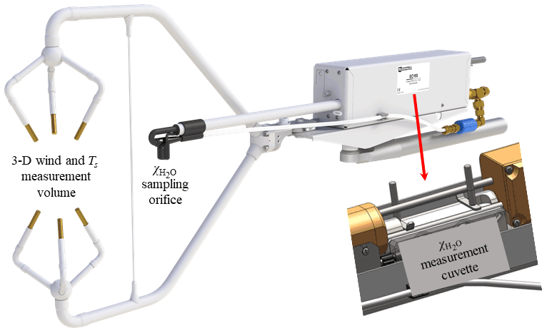
Figure 1 Measurement volume for three-dimensional (3-D) wind and sonic temperature (T_s), sampling orifice for the H₂O molar mixing ratio (${\mathit{\chi }}_{{\mathrm{H}}_{\mathrm{2}}\mathrm{O}}$), and measurement cuvette for ${\mathit{\chi }}_{{\mathrm{H}}_{\mathrm{2}}\mathrm{O}}$ in the CPEC300 series (Campbell Scientific Inc., UT, USA).

In this paper, the authors (1) derive a T equation in terms of T_s and χ_w based on first principles as an alternative to the commonly used equations that are based on approximations, (2) estimate and verify the accuracy of the first-principles T, (3) assess the expected advantages of the first-principles T as a high-frequency signal insensitive to solar contamination suffered by conventional T sensor measurements (Lin et al., 2001; Blonquist and Bugbee, 2018), and (4) brief the potential applications of the derived T equation in flux measurements. We first provide a summary of the moist turbulence thermodynamics of the boundary-layer flows measured by CPEC flux systems.

2 Background

A CPEC system is commonly used to measure boundary-layer flows for the CO₂, H₂O, heat, and momentum fluxes between ecosystems and the atmosphere. Such a system is equipped with a 3-D sonic anemometer to measure the speed of sound in three dimensions in the central open space of the instrument (hereafter referred to as open space), from which can be calculated T_s and 3-D components of wind with a fast response. Integrated with this sonic anemometer, a fast-response infrared analyzer concurrently measures CO₂ and H₂O in its cuvette (closed space) of infrared measurements, through which air is sampled under pump pressure while being heated (Fig. 1). The analyzer outputs the CO₂ mixing ratio (i.e., ${\mathit{\chi }}_{{\mathrm{CO}}_{\mathrm{2}}}={\mathit{\rho }}_{{\mathrm{CO}}_{\mathrm{2}}}/{\mathit{\rho }}_{\mathrm{d}}$, where ${\mathit{\rho }}_{{\mathrm{CO}}_{\mathrm{2}}}$ is CO₂ density and ρ_d is dry-air density) and χ_w (i.e., ${\mathit{\rho }}_{\mathrm{w}}/{\mathit{\rho }}_{\mathrm{d}}$). Together, these instruments provide high-frequency (e.g., 10 Hz) measurements from which the fluxes are computed (Aubinet et al., 2012) at a point represented by the sampling space of the CPEC system.

These basic high-frequency measurements of 3-D wind speed, T_s, χ_w, and ${\mathit{\chi }}_{{\mathrm{CO}}_{\mathrm{2}}}$ provide observations from which mean and fluctuation properties of air, such as ρ_d, ρ, ρ_w, and ${\mathit{\rho }}_{{\mathrm{CO}}_{\mathrm{2}}}$, and, hence, fluxes can be determined. For instance, water vapor flux is calculated from ${\overline{\mathit{\rho }}}_{\mathrm{d}}\stackrel{\mathrm{‾}}{w^{\prime }{\mathit{\chi }}_{\mathrm{w}}^{\prime }}$, where w is the vertical velocity of air, and the prime indicates the fluctuation of the variable away from its mean as indicated by the overbar (e.g., $w^{\prime }=w-\overline{w}$). Given the measurements of χ_w and P from CPEC systems and based on the gas laws (Wallace and Hobbs, 2006), ρ_d is derived from

$$\begin{array}{}\text{(1)}& {\mathit{\rho }}_{\mathrm{d}}={\displaystyle \frac{P}{T\left(R_{\mathrm{d}}+R_{\mathrm{v}}{\mathit{\chi }}_{\mathrm{w}}\right)}},\end{array}$$

where R_d is the gas constant for dry air and R_v is the gas constant for water vapor. In turn, ρ_w is equal to ρ_dχ_w and ρ is a sum of ρ_d and ρ_w. All mentioned physical properties can be derived if T in Eq. (1) for ρ_d is acquired.

Additionally, equations for ecosystem exchange and flux require ${\overline{\mathit{\rho }}}_{\mathrm{d}}$ (Gu et al., 2012) and $\stackrel{\mathrm{‾}}{{\mathit{\rho }}_{\mathrm{d}}w}$ (Foken et al., 2012). Furthermore, due to accuracy limitations in measurements of w from a modern sonic anemometer, the dry-air flux of $\stackrel{\mathrm{‾}}{{\mathit{\rho }}_{\mathrm{d}}w}$ must be derived from $\stackrel{\mathrm{‾}}{{\mathit{\rho }}_{\mathrm{d}}^{\prime }{w}^{\prime }}-{\overline{\mathit{\rho }}}_{\mathrm{d}}\overline{w}$ (Webb et al., 1980; Lee and Massman, 2011). Because of its role in flux measurements, a high-frequency representation of ρ_d is needed. To acquire such a ρ_d from Eq. (1) for advanced applications, high-frequency T in temporal synchronization with χ_w and P is needed.

In a modern CPEC system, P is measured using a fast-response barometer suitable for measurements at a high frequency (e.g., 10 Hz; Campbell Scientific Inc., 2018a), and, as discussed above, χ_w is a high-frequency signal from a fast-response infrared analyzer (e.g., commonly up to 20 Hz). If T is measured using a slow-response sensor, the three independent variables in Eq. (1) do not have equivalent synchronicity in their frequency response. In terms of frequency response, ${\mathit{\rho }}_{\mathrm{d}}^{\prime }$ cannot be correctly acquired. ${\overline{\mathit{\rho }}}_{\mathrm{d}}$ derived based on Eq. (1) also has uncertainty, although it can be approximated from either of the two following equations:

$$\begin{array}{}\text{(2)}& {\overline{\mathit{\rho }}}_{\mathrm{d}}=\stackrel{\mathrm{‾}}{{\displaystyle \frac{P}{T\left(R_{\mathrm{d}}+R_{\mathrm{v}}{\mathit{\chi }}_{\mathrm{w}}\right)}}}\end{array}$$

and

$$\begin{array}{}\text{(3)}& {\overline{\mathit{\rho }}}_{\mathrm{d}}={\displaystyle \frac{\overline{P}}{\overline{T}\left(R_{\mathrm{d}}+R_{\mathrm{v}}{\overline{\mathit{\chi }}}_{\mathrm{w}}\right)}}.\end{array}$$

Equation (2) is mathematically valid in averaging rules (Stull, 1988), but the response of the system to T is slower than to χ_w and even P, while Eq. (3) is invalid under averaging rules, although its three overbar independent variables can be evaluated over an average interval. Consequently, neither $\stackrel{\mathrm{‾}}{{\mathit{\rho }}_{\mathrm{d}}w}$ nor ${\overline{\mathit{\rho }}}_{\mathrm{d}}$ can be evaluated strictly in theory.

Measurements of T at a high frequency (similarly to those at a low frequency) are contaminated by solar radiation, even under shields (Lin et al., 2001) and when aspirated (Campbell Scientific Inc., 2010; R.M. Young Company, 2004; Apogee Instruments Inc., 2013; Blonquist and Bugbee, 2018). Although a naturally ventilated or fan-aspirated radiation shield could ensure the accuracy of a conventional (i.e., slow-response) thermometer often within ±0.2 K at 0 ^∘C (Harrison and Burt, 2021) to satisfy the standard for conventional T measurement as required by the World Meteorological Organization (WMO, 2018), the aspiration shield method cannot acquire T at a high frequency due to the disturbance of an aspiration fan and the blockage of a shield to natural turbulent flows. Additionally, fine wires have limited applicability for long-term measurements in rugged field conditions typically encountered in ecosystem monitoring.

To avoid the issues above in use of either slow- or fast-response T sensors under field conditions, deriving T from T_s and χ_w (Schotanus et al., 1983; Kaimal and Gaynor, 1991) is an advantageous alternative to the applications of T in CPEC measurements and is a significant technology for instrumentation to pursue. In a CPEC system, T_s is measured at a high frequency (e.g., 10 Hz) using a fast-response sonic anemometer to detect the speed of sound in the open space (Munger et al., 2012), provided there is no evidence of contamination by solar radiation. It is a high-frequency signal. χ_w is measured at the same frequency as for T_s using an infrared analyzer equivalent to the sonic anemometer with a high-frequency response time (Ma et al., 2017). χ_w reported from a CPEC system is converted from water vapor molar density measured inside the closed-space cuvette, whose internal pressure and internal temperature are more stable than P and T in the open space and can be more accurately measured. Because of this, solar warming and radiation cooling of the cuvette is irrelevant, as long as water molar density, pressure, and temperature inside the closed-space cuvette are more accurately measured. Therefore, it could be reasonably expected that T calculated from T_s and χ_w in a CPEC system should be a high-frequency signal insensitive to solar radiation.

The first of two equations commonly used to compute T from T_s and air-moisture-related variables is given by Schotanus et al. (1983) as

$$\begin{array}{}\text{(4)}& T=T_{\mathrm{s}}{\left(\mathrm{1}+\mathrm{0.51}q\right)}^{-\mathrm{1}},\end{array}$$

where q is specific humidity, defined as a ratio of water vapor to moist-air density. The second equation is given by Kaimal and Gaynor (1991) as

$$\begin{array}{}\text{(5)}& T=T_{\mathrm{s}}{\left(\mathrm{1}+\mathrm{0.32}{\displaystyle \frac{e}{P}}\right)}^{-\mathrm{1}},\end{array}$$

where e is water vapor pressure. Rearranging these two equations gives T in terms of T_s and χ_w. Expressing q in terms of ρ_d and ρ_w, Eq. (4) becomes

$$\begin{array}{}\text{(6)}& \begin{array}{rl}T& =T_{\mathrm{s}}{\left(\mathrm{1}+\mathrm{0.51}{\displaystyle \frac{{\mathit{\rho }}_{\mathrm{w}}}{{\mathit{\rho }}_{\mathrm{d}}+{\mathit{\rho }}_{\mathrm{w}}}}\right)}^{-\mathrm{1}}\\ & =T_{\mathrm{s}}{\left(\mathrm{1}+\mathrm{0.51}{\displaystyle \frac{{\mathit{\chi }}_{\mathrm{w}}}{\mathrm{1}+{\mathit{\chi }}_{\mathrm{w}}}}\right)}^{-\mathrm{1}},\end{array}\end{array}$$

and expressing e and P using the equation of state, Eq. (5) becomes

$$\begin{array}{}\text{(7)}& \begin{array}{rl}T& =T_{\mathrm{s}}{\left(\mathrm{1}+\mathrm{0.32}{\displaystyle \frac{R_{\mathrm{v}}T{\mathit{\rho }}_{\mathrm{w}}}{R_{\mathrm{d}}T{\mathit{\rho }}_{\mathrm{d}}+R_{\mathrm{v}}T{\mathit{\rho }}_{\mathrm{w}}}}\right)}^{-\mathrm{1}}\\ & =T_{\mathrm{s}}{\left(\mathrm{1}+\mathrm{0.51}{\displaystyle \frac{{\mathit{\chi }}_{\mathrm{w}}}{\mathrm{1}+\mathrm{1.61}{\mathit{\chi }}_{\mathrm{w}}}}\right)}^{-\mathrm{1}}.\end{array}\end{array}$$

The χ_w-related terms in the denominator inside parentheses in both equations above clearly reveal that T values from the same T_s and χ_w using the two commonly used Eqs. (4) and (5) will not be the same. The absolute difference in the values (ΔT_e, i.e., the difference in T between Eqs. 4 and 5) can be analytically expressed as

$$\begin{array}{}\text{(8)}& \mathrm{\Delta }{T}_e={\displaystyle \frac{\mathrm{0.31}{T}_{\mathrm{s}}{\mathit{\chi }}_{\mathrm{w}}^{\mathrm{2}}}{\mathrm{1}+\mathrm{3.63}{\mathit{\chi }}_{\mathrm{w}}+\mathrm{3.20}{\mathit{\chi }}_{\mathrm{w}}^{\mathrm{2}}}}.\end{array}$$

Given that, in a CPEC system, the sonic anemometer has an operational range in T_s of −30 to 57 ^∘C (Campbell Scientific Inc., 2018b) and an infrared analyzer has a measurement range in χ_w of 0 to 0.045 kgH₂O kg⁻¹ (Campbell Scientific Inc., 2018a), ΔT_e ranges up to 0.177 K, which brings an uncertainty in the accuracy of T calculated from either Eq. (4) or Eq. (5) and raises the question of which equation is better.

Reviewing the sources of Eq. (4) (Schotanus et al., 1983; Swiatek, 2009; van Dijk, 2002) and Eq. (5) (Ishii, 1935; Barrett and Suomi, 1949; Kaimal and Businger, 1963; Kaimal and Gaynor, 1991), it was found that approximation procedures were used in the derivation of both equations, but the approach to the derivation of Eq. (4) (Appendix A) is different from that of Eq. (5) (Appendix B). These different approaches create a disparity between the two commonly used equations as shown in Eq. (8), and the approximation procedures lead to the controversy as to which equation is more accurate. The controversy can be avoided if the T equation in terms of T_s and χ_w can be derived from the T_s equation and first-principles equations, if possible without an approximation and verified against precision measurements of T with minimized solar contamination.

3 Theory

As discussed above, a sonic anemometer measures the speed of sound (c) concurrently with measurement of the 3-D wind speed (Munger et al., 2012). The speed of sound in the homogeneous atmospheric boundary layer is defined by Barrett and Suomi (1949) as

$$\begin{array}{}\text{(9)}& c^{\mathrm{2}}=\mathit{\gamma }{\displaystyle \frac{P}{\mathit{\rho }}},\end{array}$$

where γ is the ratio of moist-air specific heat at constant pressure (C_p) to moist-air specific heat at constant volume (C_v). Substitution of the equation of state into Eq. (9) gives T as a function of c:

$$\begin{array}{}\text{(10)}& T={\displaystyle \frac{c^{\mathrm{2}}}{\mathit{\gamma }R}}.\end{array}$$

This equation reveals the opportunity to use measured c for the T calculation; however, both γ and R depend on air humidity, which is unmeasurable by sonic anemometry itself; Eq. (10) is, therefore, not applicable for T calculations inside a sonic anemometer. Alternatively, γ is replaced with its counterpart for dry air (γ_d, 1.4003, i.e., the ratio of dry-air specific heat at constant pressure (C_pd, 1004 J K⁻¹ kg⁻¹) to dry-air specific heat at constant volume (C_vd, 717 J K⁻¹ kg⁻¹)) and R is replaced with its counterpart for dry air (R_d, 287.06 J K⁻¹ kg⁻¹, i.e., the gas constant for dry air). Both replacements make the right side of Eq. (10) become $c^{\mathrm{2}}/{\mathit{\gamma }}_{\mathrm{d}}{R}_{\mathrm{d}}$, which is no longer a measure of T. However, γ_d and R_d are close to their respective values of γ and R in magnitude, and, after the replacements, the right side of Eq. (10) is defined as sonic temperature (T_s), given by (Campbell Scientific Inc., 2018b)

$$\begin{array}{}\text{(11)}& T_{\mathrm{s}}={\displaystyle \frac{c^{\mathrm{2}}}{{\mathit{\gamma }}_{\mathrm{d}}{R}_{\mathrm{d}}}}.\end{array}$$

Comparing this equation to Eq. (10), given c, if air is dry, T must be equal to T_s; therefore, the authors state that “sonic temperature of moist air is the temperature that its dry-air component reaches when moist air has the same enthalpy.” Since both γ_d and R_d are constants and c is measured by a sonic anemometer and corrected for the crosswind effect inside the sonic anemometer based on its 3-D wind measurements (Liu et al., 2001; Zhou et al., 2018), Eq. (11) is used inside the operating system (OS) of modern sonic anemometers to report T_s instead of T.

Equations (9) to (11) provide a theoretical basis of first principles to derive the relationship of T to T_s and χ_w. In Eq. (9), γ and ρ vary with air humidity and P is related to ρ as described by the equation of state. Consequently, the derivation of T from T_s and χ_w for CPEC systems needs to address the relationship of γ, ρ, and P to air humidity in terms of χ_w.

3.1 Relationship of γ to χ_w

For moist air, the ratio of specific heat at constant pressure to specific heat at constant volume is

$$\begin{array}{}\text{(12)}& \mathit{\gamma }={\displaystyle \frac{C_{\mathrm{p}}}{C_{\mathrm{v}}}},\end{array}$$

where C_p varies with air moisture between C_pd and C_pw (water vapor specific heat at constant pressure, 1952 J kg⁻¹ K⁻¹). It is the arithmetical average of C_pd and C_pw weighted by the dry air mass and water vapor mass, respectively, given by (Stull, 1988; Swiatek, 2009)

$$\begin{array}{}\text{(13)}& C_{\mathrm{p}}={\displaystyle \frac{C_{\mathrm{pd}}{\mathit{\rho }}_{\mathrm{d}}+C_{\mathrm{pw}}{\mathit{\rho }}_{\mathrm{w}}}{{\mathit{\rho }}_{\mathrm{d}}+{\mathit{\rho }}_{\mathrm{w}}}}.\end{array}$$

Based on the same rationale, C_v is

$$\begin{array}{}\text{(14)}& C_{\mathrm{v}}={\displaystyle \frac{C_{\mathrm{vd}}{\mathit{\rho }}_{\mathrm{d}}+C_{\mathrm{vw}}{\mathit{\rho }}_{\mathrm{w}}}{{\mathit{\rho }}_{\mathrm{d}}+{\mathit{\rho }}_{\mathrm{w}}}},\end{array}$$

where C_vw is the specific heat of water vapor at constant volume (1463 J kg⁻¹ K⁻¹). Substituting Eqs. (13) and (14) into Eq. (12) generates

$$\begin{array}{}\text{(15)}& \mathit{\gamma }={\mathit{\gamma }}_{\mathrm{d}}{\displaystyle \frac{\mathrm{1}+\left(C_{\mathrm{pw}}/C_{\mathrm{pd}}\right){\mathit{\chi }}_{\mathrm{w}}}{\mathrm{1}+\left(C_{\mathrm{vw}}/C_{\mathrm{vd}}\right){\mathit{\chi }}_{\mathrm{w}}}}.\end{array}$$

3.2 Relationship of $P/\mathit{\rho }$ to χ_w

Atmospheric P is the sum of P_d and e. Similarly, ρ is the sum of ρ_d and ρ_w. Using the equation of state, the ratio of P to ρ can be expressed as

$$\begin{array}{}\text{(16)}& {\displaystyle \frac{P}{\mathit{\rho }}}={\displaystyle \frac{R_{\mathrm{d}}T{\mathit{\rho }}_{\mathrm{d}}+R_{\mathrm{v}}T{\mathit{\rho }}_{\mathrm{w}}}{{\mathit{\rho }}_{\mathrm{d}}+{\mathit{\rho }}_{\mathrm{w}}}}={\displaystyle \frac{R_{\mathrm{d}}T\left(\mathrm{1}+\frac{R_{\mathrm{v}}}{R_{\mathrm{d}}}{\mathit{\chi }}_{\mathrm{w}}\right)}{\mathrm{1}+{\mathit{\chi }}_{\mathrm{w}}}}.\end{array}$$

In this equation, the ratio of R_v to R_d is given by

$$\begin{array}{}\text{(17)}& {\displaystyle \frac{R_{\mathrm{v}}}{R_{\mathrm{d}}}}={\displaystyle \frac{R^{\ast }/M_{\mathrm{w}}}{R^{\ast }/M_{\mathrm{d}}}}={\displaystyle \frac{\mathrm{1}}{M_{\mathrm{w}}/M_{\mathrm{d}}}},\end{array}$$

where R^∗ is the universal gas constant, M_w is the molecular mass of water vapor (18.0153 kg kmol⁻¹), and M_d is the molecular mass of dry air (28.9645 kg kmol⁻¹). The ratio of M_w to M_d is 0.622, conventionally denoted by ε. Substituting Eq. (17), after its denominator is represented by ε, into Eq. (16) leads to

$$\begin{array}{}\text{(18)}& {\displaystyle \frac{P}{\mathit{\rho }}}={\displaystyle \frac{R_{\mathrm{d}}T\left(\mathit{\epsilon }+{\mathit{\chi }}_{\mathrm{w}}\right)}{\mathit{\epsilon }\left(\mathrm{1}+{\mathit{\chi }}_{\mathrm{w}}\right)}}.\end{array}$$

3.3 Relationship of T_s to T and χ_w

Substituting Eqs. (15) and (18) into Eq. (9), c² is expressed in terms of T and χ_w along with atmospheric physics constants:

$$\begin{array}{}\text{(19)}& c^{\mathrm{2}}={\displaystyle \frac{R_{\mathrm{d}}{\mathit{\gamma }}_{\mathrm{d}}T\left(\mathit{\epsilon }+{\mathit{\chi }}_{\mathrm{w}}\right)\left[\mathrm{1}+\left(C_{\mathrm{pw}}/C_{\mathrm{pd}}\right){\mathit{\chi }}_{\mathrm{w}}\right]}{\mathit{\epsilon }\left(\mathrm{1}+{\mathit{\chi }}_{\mathrm{w}}\right)\left[\mathrm{1}+\left(C_{\mathrm{vw}}/C_{\mathrm{vd}}\right){\mathit{\chi }}_{\mathrm{w}}\right]}}.\end{array}$$

Further, substituting c² into Eq. (11) generates

$$\begin{array}{}\text{(20)}& T_{\mathrm{s}}=T{\displaystyle \frac{\left(\mathit{\epsilon }+{\mathit{\chi }}_{\mathrm{w}}\right)\left[\mathrm{1}+\left(C_{\mathrm{pw}}/C_{\mathrm{pd}}\right){\mathit{\chi }}_{\mathrm{w}}\right]}{\mathit{\epsilon }\left(\mathrm{1}+{\mathit{\chi }}_{\mathrm{w}}\right)\left[\mathrm{1}+\left(C_{\mathrm{vw}}/C_{\mathrm{vd}}\right){\mathit{\chi }}_{\mathrm{w}}\right]}}.\end{array}$$

This Eq. (20) now expresses T_s in terms of the T of interest to this study, χ_w measured in CPEC systems, and atmospheric physics constants (i.e., ε, C_pw, C_pd, C_vw, and C_vd).

3.4 Air temperature equation

Rearranging the terms in Eq. (20) results in

$$\begin{array}{}\text{(21)}& T=T_{\mathrm{s}}{\displaystyle \frac{\mathit{\epsilon }\left(\mathrm{1}+{\mathit{\chi }}_{\mathrm{w}}\right)\left[\mathrm{1}+\left(C_{\mathrm{vw}}/C_{\mathrm{vd}}\right){\mathit{\chi }}_{\mathrm{w}}\right]}{\left(\mathit{\epsilon }+{\mathit{\chi }}_{\mathrm{w}}\right)\left[\mathrm{1}+\left(C_{\mathrm{pw}}/C_{\mathrm{pd}}\right){\mathit{\chi }}_{\mathrm{w}}\right]}}.\end{array}$$

This equation shows that T is a function of T_s and χ_w that are measured at a high frequency in a CPEC system by a sonic anemometer and an infrared analyzer.

A CPEC system outputs the water vapor molar mixing ratio (Campbell Scientific Inc., 2018a) commonly used in the community of eddy-covariance fluxes (AmeriFlux, 2018). The relation of water vapor mass to the molar mixing ratio (${\mathit{\chi }}_{{\mathrm{H}}_{\mathrm{2}}\mathrm{O}}$ in molH₂O mol⁻¹) is given by

$$\begin{array}{}\text{(22)}& {\mathit{\chi }}_{\mathrm{w}}={\displaystyle \frac{M_{\mathrm{w}}}{M_{\mathrm{d}}}}{\mathit{\chi }}_{{\mathrm{H}}_{\mathrm{2}}\mathrm{O}}=\mathit{\epsilon }{\mathit{\chi }}_{{\mathrm{H}}_{\mathrm{2}}\mathrm{O}}.\end{array}$$

Substituting this relation into Eq. (21) and denoting $C_{\mathrm{vw}}/C_{\mathrm{vd}}$ with γ_v = 2.04045 and $C_{\mathrm{pw}}/C_{\mathrm{pd}}$ with γ_p=1.94422, Eq. (21) is expressed as

$$\begin{array}{}\text{(23)}& T=T_{\mathrm{s}}{\displaystyle \frac{\left(\mathrm{1}+\mathit{\epsilon }{\mathit{\chi }}_{{\mathrm{H}}_{\mathrm{2}}\mathrm{O}}\right)\left(\mathrm{1}+\mathit{\epsilon }{\mathit{\gamma }}_{\mathrm{v}}{\mathit{\chi }}_{{\mathrm{H}}_{\mathrm{2}}\mathrm{O}}\right)}{\left(\mathrm{1}+{\mathit{\chi }}_{{\mathrm{H}}_{\mathrm{2}}\mathrm{O}}\right)\left(\mathrm{1}+\mathit{\epsilon }{\mathit{\gamma }}_{\mathrm{p}}{\mathit{\chi }}_{{\mathrm{H}}_{\mathrm{2}}\mathrm{O}}\right)}}.\end{array}$$

This is the air temperature equation in terms of T_s and ${\mathit{\chi }}_{{\mathrm{H}}_{\mathrm{2}}\mathrm{O}}$ for use in CPEC systems. It is derived from a theoretical basis of first principles (i.e., Eqs. 9 to 11). In its derivation, except for the use of the equation of state and Dalton's law, no other assumptions or approximations are used. Therefore, Eq. (23) is an exact equation of T in terms of T_s and ${\mathit{\chi }}_{{\mathrm{H}}_{\mathrm{2}}\mathrm{O}}$ for the turbulent airflow sampled through a CPEC system and thus avoids the controversy in the use of Eqs. (4) and (5) arising from approximations, as shown in Appendices A and B. Therefore, T computed from this equation (hereafter referred to as equation-computed T) should be accurate, as long as the values of T_s and ${\mathit{\chi }}_{{\mathrm{H}}_{\mathrm{2}}\mathrm{O}}$ are exact.

For this study, however, T_s and ${\mathit{\chi }}_{{\mathrm{H}}_{\mathrm{2}}\mathrm{O}}$ are measured by the CPEC systems deployed in the field under changing weather conditions through four seasons. Their measured values must include measurement uncertainty in T_s, denoted by ΔT_s, and in ${\mathit{\chi }}_{{\mathrm{H}}_{\mathrm{2}}\mathrm{O}}$ as well, denoted by $\mathrm{\Delta }{\mathit{\chi }}_{{\mathrm{H}}_{\mathrm{2}}\mathrm{O}}$. The uncertainties, ΔT_s and/or $\mathrm{\Delta }{\mathit{\chi }}_{{\mathrm{H}}_{\mathrm{2}}\mathrm{O}}$, unavoidably propagate to create uncertainty in equation-computed T, denoted by ΔT, which makes an exact T impossible. In numerical analysis (Burden and Faires, 1993) or in statistics (Snedecor and Cochran, 1989), any applicable equation requires the specification of an uncertainty term. Therefore, the equations for T should include a specification of their respective uncertainty expressed as the bounds (i.e., the maximum and minimum limits) specifying the range of the equation-computed T that need to be known for any application. According to the definition of accuracy that was advanced by the International Organization for Standardization (2012), this uncertainty range is equivalent to the “accuracy” of the range contributed by both systematic errors (trueness) and random variability (precision). Apparently, ΔT_s is the accuracy of T_s measurements and $\mathrm{\Delta }{\mathit{\chi }}_{{\mathrm{H}}_{\mathrm{2}}\mathrm{O}}$ is the accuracy of ${\mathit{\chi }}_{{\mathrm{H}}_{\mathrm{2}}\mathrm{O}}$ measurements. Both should be evaluated from their respective measurement uncertainties. The accuracy of equation-computed T is ΔT. It should be specified through its relationship to ΔT_s and $\mathrm{\Delta }{\mathit{\chi }}_{{\mathrm{H}}_{\mathrm{2}}\mathrm{O}}$.

3.5 Relationship of ΔT to ΔT_s and $\mathrm{\Delta }{\mathit{\chi }}_{{\mathrm{H}}_{\mathrm{2}}\mathrm{O}}$

As measurement accuracies, ΔT_s and $\mathrm{\Delta }{\mathit{\chi }}_{{\mathrm{H}}_{\mathrm{2}}\mathrm{O}}$ can be reasonably considered small increments in a calculus sense. As such, depending on both small increments, ΔT is the total differential of T with respect to T_s and ${\mathit{\chi }}_{{\mathrm{H}}_{\mathrm{2}}\mathrm{O}}$, given by

$$\begin{array}{}\text{(24)}& \mathrm{\Delta }T={\displaystyle \frac{\partial T}{\partial T_{\mathrm{s}}}}\mathrm{\Delta }{T}_{\mathrm{s}}+{\displaystyle \frac{\partial T}{\partial {\mathit{\chi }}_{{\mathrm{H}}_{\mathrm{2}}\mathrm{O}}}}\mathrm{\Delta }{\mathit{\chi }}_{{\mathrm{H}}_{\mathrm{2}}\mathrm{O}}.\end{array}$$

The two partial derivatives on the right side of this equation can be derived from Eq. (23). Substituting the two partial derivatives into this equation leads to

$$\begin{array}{}\text{(25)}& \begin{array}{rl}\mathrm{\Delta }T=& {\displaystyle \frac{T}{T_{\mathrm{s}}}}\mathrm{\Delta }{T}_{\mathrm{s}}+T\left[{\displaystyle \frac{\mathit{\epsilon }+\mathit{\epsilon }{\mathit{\gamma }}_{\mathrm{v}}\left(\mathrm{1}+\mathrm{2}\mathit{\epsilon }{\mathit{\chi }}_{{\mathrm{H}}_{\mathrm{2}}\mathrm{O}}\right)}{\left(\mathrm{1}+\mathit{\epsilon }{\mathit{\chi }}_{{\mathrm{H}}_{\mathrm{2}}\mathrm{O}}\right)\left(\mathrm{1}+\mathit{\epsilon }{\mathit{\gamma }}_{\mathrm{v}}{\mathit{\chi }}_{{\mathrm{H}}_{\mathrm{2}}\mathrm{O}}\right)}}\right.\\ & \left.-{\displaystyle \frac{\mathrm{1}+\mathit{\epsilon }{\mathit{\gamma }}_{\mathrm{p}}\left(\mathrm{1}+\mathrm{2}{\mathit{\chi }}_{{\mathrm{H}}_{\mathrm{2}}\mathrm{O}}\right)}{\left(\mathrm{1}+{\mathit{\chi }}_{{\mathrm{H}}_{\mathrm{2}}\mathrm{O}}\right)\left(\mathrm{1}+\mathit{\epsilon }{\mathit{\gamma }}_{\mathrm{p}}{\mathit{\chi }}_{{\mathrm{H}}_{\mathrm{2}}\mathrm{O}}\right)}}\right]\mathrm{\Delta }{\mathit{\chi }}_{{\mathrm{H}}_{\mathrm{2}}\mathrm{O}}.\end{array}\end{array}$$

This equation indicates that in dry air when T=T_s, ΔT is equal to ΔT_s if ${\mathit{\chi }}_{{\mathrm{H}}_{\mathrm{2}}\mathrm{O}}$ is measured accurately (i.e., $\mathrm{\Delta }{\mathit{\chi }}_{{\mathrm{H}}_{\mathrm{2}}\mathrm{O}}=\mathrm{0}$ while ${\mathit{\chi }}_{{\mathrm{H}}_{\mathrm{2}}\mathrm{O}}=$ 0). However, air in the atmospheric boundary layer where CPEC systems are used is always moist. Given this equation, ΔT at T_s and ${\mathit{\chi }}_{{\mathrm{H}}_{\mathrm{2}}\mathrm{O}}$ can be evaluated by using ΔT_s and $\mathrm{\Delta }{\mathit{\chi }}_{{\mathrm{H}}_{\mathrm{2}}\mathrm{O}}$, both of which are related to the measurement specifications of sonic anemometers for T_s (Campbell Scientific Inc., 2018b) and of infrared analyzers for ${\mathit{\chi }}_{{\mathrm{H}}_{\mathrm{2}}\mathrm{O}}$ (Campbell Scientific Inc., 2018a). Sonic anemometers and infrared analyzers with different models and brands have different specifications from their manufacturers. The manufacturer of the anemometer we studied (Fig. 1) employs carbon fiber with minimized thermo-expansion and thermo-contraction for sonic strut stability (via personal communication with CSAT structural designer Antoine Rousseau, 2021); structural design with optimized sonic volume for less aerodynamic disturbance (Fig. 1); and advanced proprietary sonic firmware for more accurate measurements (Zhou et al., 2018), which reduces the variability in T_s by several kelvins compared to what has been reported for sonics from other models (Mauder and Zeeman, 2018). Any combination of sonic and infrared instruments has a combination of ΔT_s and $\mathrm{\Delta }{\mathit{\chi }}_{{\mathrm{H}}_{\mathrm{2}}\mathrm{O}}$, which are specified by their manufacturers. In turn, from Eq. (25), the combination generates ΔT of equation-computed T for the corresponding combination of the sonic and infrared instruments with given models and brands. Therefore, Eqs. (23) and (25) are applicable to any CPEC system beyond the brand of our study (Fig. 1). The applicability of Eq. (23) for any sonic or infrared instrument can be assessed based on ΔT against the required T accuracy for a specific application.

On the right side of Eq. (25), the first term with ΔT_s can be expressed as $\mathrm{\Delta }{T}_{T_{\mathrm{s}}}$ (i.e., uncertainty portion of ΔT due to ΔT_s) and the second term with $\mathrm{\Delta }{\mathit{\chi }}_{{\mathrm{H}}_{\mathrm{2}}\mathrm{O}}$ can be expressed as $\mathrm{\Delta }{T}_{{\mathit{\chi }}_{{\mathrm{H}}_{\mathrm{2}}\mathrm{O}}}$ (i.e., uncertainty portion of ΔT due to $\mathrm{\Delta }{\mathit{\chi }}_{{\mathrm{H}}_{\mathrm{2}}\mathrm{O}}$). Using $\mathrm{\Delta }{T}_{T_{\mathrm{s}}}$ and $\mathrm{\Delta }{T}_{{\mathit{\chi }}_{{\mathrm{H}}_{\mathrm{2}}\mathrm{O}}}$, this equation can be simplified as

$$\begin{array}{}\text{(26)}& \mathrm{\Delta }T=\mathrm{\Delta }{T}_{T_{\mathrm{s}}}+\mathrm{\Delta }{T}_{{\mathit{\chi }}_{{\mathrm{H}}_{\mathrm{2}}\mathrm{O}}}.\end{array}$$

Assessment of the accuracy of equation-computed T is to evaluate $\mathrm{\Delta }{T}_{T_{\mathrm{s}}}$ and $\mathrm{\Delta }{T}_{{\mathit{\chi }}_{{\mathrm{H}}_{\mathrm{2}}\mathrm{O}}}$ correspondingly from ΔT_s and $\mathrm{\Delta }{\mathit{\chi }}_{{\mathrm{H}}_{\mathrm{2}}\mathrm{O}}$.

4 Accuracy

The CPEC system for this study is CPEC310 (Campbell Scientific Inc., UT, USA), whose major components are a CSAT3A sonic anemometer (updated version in 2016) for a fast response to 3-D wind and T_s and an EC155 infrared analyzer for a fast response to H₂O along with CO₂ (Burgon et al., 2015; Ma et al., 2017). The system operates in a T range of −30 to 50 ^∘C and measures ${\mathit{\chi }}_{{\mathrm{H}}_{\mathrm{2}}\mathrm{O}}$ in a range up to 79 mmolH₂O mol⁻¹ (i.e., 37 ^∘C dew point temperature at 86 kPa in manufacturer environment); therefore, the accuracy of equation-computed T, depending on ΔT_s and $\mathrm{\Delta }{\mathit{\chi }}_{{\mathrm{H}}_{\mathrm{2}}\mathrm{O}}$, should be defined and estimated in a domain over both ranges.

4.1 ΔT_s (measurement accuracy in T_s)

As is true for other sonic anemometers (e.g., Gill Instruments, 2004), the CSAT3A has not been assigned a T_s measurement performance (Campbell Scientific Inc., 2018b) because the theories and methodologies of how to specify this performance, to the best of our knowledge, have not been clearly defined. The performance of the CSAT series for T_s is best near the production temperature at around 20 ^∘C and drifts a little away from this temperature. Within the operational range of a CPEC system in ambient air temperature, the updated version of CSAT3A has an overall uncertainty of ±1.00 ^∘C (i.e., |ΔT_s|<1.00 K, via personal communication with CSAT authority Larry Jacobsen through email in 2017 and in person in 2018).

4.2 $\mathrm{\Delta }{\mathit{\chi }}_{{\mathrm{H}}_{\mathrm{2}}\mathrm{O}}$ (measurement accuracy in ${\mathit{\chi }}_{{\mathrm{H}}_{\mathrm{2}}\mathrm{O}}$)

The accuracy in H₂O measurements from infrared analyzers depends upon analyzer measurement performance. This performance is specified using four component uncertainties: (1) precision variability (${\mathit{\sigma }}_{{\mathrm{H}}_{\mathrm{2}}\mathrm{O}}$), (2) maximum zero drift range with ambient air temperature (d_wz), (3) maximum gain drift with ambient air temperature (±${\mathit{\delta }}_{{\mathrm{H}}_{\mathrm{2}}\mathrm{O}}{\mathit{\chi }}_{{\mathrm{H}}_{\mathrm{2}}\mathrm{O}}$, where ${\mathit{\delta }}_{{\mathrm{H}}_{\mathrm{2}}\mathrm{O}}$ is the gain drift percentage), and (4) cross-sensitivity to CO₂ (s_c) (LI-COR Biosciences, 2016; Campbell Scientific Inc., 2018c). Zhou et al. (2021) composited the four component uncertainties as an accuracy model formulated as the H₂O accuracy equation for CPEC systems applied in ecosystems, given by

$$\begin{array}{}\text{(27)}& \begin{array}{rl}\mathrm{\Delta }{\mathit{\chi }}_{{\mathrm{H}}_{\mathrm{2}}\mathrm{O}}=& \pm \left[\mathrm{1.96}{\mathit{\sigma }}_{{\mathrm{H}}_{\mathrm{2}}\mathrm{O}}+\mathrm{585}\left|s_{\mathrm{c}}\right|+{\displaystyle \frac{\left|d_{\mathrm{wz}}\right|+{\mathit{\delta }}_{{\mathrm{H}}_{\mathrm{2}}\mathrm{O}\mathrm{\_}\mathrm{g}}{\mathit{\chi }}_{{\mathrm{H}}_{\mathrm{2}}\mathrm{O}}}{T_{\mathrm{rh}}-T_{\mathrm{rl}}}}\right.\\ & \left.\times \left\{\begin{array}{ll}{T}_{\mathrm{c}}-T& T_{\mathrm{c}}>T>T_{\mathrm{rl}}\\ T-T_{\mathrm{c}}& T_{\mathrm{c}}<T<T_{\mathrm{rh}}\end{array}\right.\right],\end{array}\end{array}$$

where T_c is the ambient air temperature at which an infrared analyzer was calibrated by the manufacturer to fit its working equation or zeroed/spanned by a user in the field to adjust the zero/gain drift; subscripts rh and rl indicate the range of the highest and lowest values, respectively; and T_rh and T_rl are the highest and lowest T, respectively, over the operational range in T of CPEC systems. Given the infrared analyzer specifications – ${\mathit{\sigma }}_{{\mathrm{H}}_{\mathrm{2}}\mathrm{O}}$, s_c, d_wz, ${\mathit{\delta }}_{{\mathrm{H}}_{\mathrm{2}}\mathrm{O}\mathrm{\_}\mathrm{g}}$, T_rl, and T_rh – this equation can be used to estimate $\mathrm{\Delta }{\mathit{\chi }}_{{\mathrm{H}}_{\mathrm{2}}\mathrm{O}}$ in Eq. (25) and eventually $\mathrm{\Delta }{T}_{{\mathit{\chi }}_{{\mathrm{H}}_{\mathrm{2}}\mathrm{O}}}$ in Eq. (26) over the domain of T and ${\mathit{\chi }}_{{\mathrm{H}}_{\mathrm{2}}\mathrm{O}}$.

4.3 ΔT (accuracy of equation-computed T)

The accuracy of equation-computed T can be evaluated using ΔT_s and $\mathrm{\Delta }{\mathit{\chi }}_{{\mathrm{H}}_{\mathrm{2}}\mathrm{O}}$ (Eq. 25), varying with T, T_s, and ${\mathit{\chi }}_{{\mathrm{H}}_{\mathrm{2}}\mathrm{O}}$. Both T and T_s reflect air temperature, being associated with each other through ${\mathit{\chi }}_{{\mathrm{H}}_{\mathrm{2}}\mathrm{O}}$ (Eq. 23). Given ${\mathit{\chi }}_{{\mathrm{H}}_{\mathrm{2}}\mathrm{O}}$, T can be calculated from T_s, and vice versa; therefore, for the figure presentations in this study, it is sufficient to use either T or T_s, instead of both, to show ΔT with air temperature. Considering T to be of interest to this study, T will be used. As such, ΔT can be analyzed over a domain of T and ${\mathit{\chi }}_{{\mathrm{H}}_{\mathrm{2}}\mathrm{O}}$ within the operational range in T of CPEC systems from −30 to 50 ^∘C across the analyzer measurement range of ${\mathit{\chi }}_{{\mathrm{H}}_{\mathrm{2}}\mathrm{O}}$ from 0 to 0.079 molH₂O mol⁻¹.

To visualize the relationship of ΔT with T and ${\mathit{\chi }}_{{\mathrm{H}}_{\mathrm{2}}\mathrm{O}}$, ΔT is presented better as the ordinate along T and as the abscissa associated with ${\mathit{\chi }}_{{\mathrm{H}}_{\mathrm{2}}\mathrm{O}}$. However, due to the positive dependence of air water vapor saturation on T (Wallace and Hobbs, 2006), ${\mathit{\chi }}_{{\mathrm{H}}_{\mathrm{2}}\mathrm{O}}$ has a range that is wider at a higher T and narrower at a lower T. To present ΔT over the same measure of air moisture, even at different T values, the saturation water vapor pressure is used to scale air moisture to 0, 20, 40, 60, 80, and 100 (i.e., RH, relative humidity in %). For each scaled RH value, ${\mathit{\chi }}_{{\mathrm{H}}_{\mathrm{2}}\mathrm{O}}$ can be calculated at different T and P values (Appendix C) for use in Eq. (25). In this way, over the range of T, the trend of ΔT due to each measurement uncertainty source can be shown along the curves with equal RH as the measure of air moisture (Fig. 2).

Figure 2 Accuracy of air temperature computed from Eq. (23) (equation-computed T) over the measurement range of the H₂O molar mixing ratio (${\mathit{\chi }}_{{\mathrm{H}}_{\mathrm{2}}\mathrm{O}}$) within the operational range of T for the CPEC300 series (Campbell Scientific Inc., UT, USA): (a) accuracy component of equation-computed T due to sonic temperature (T_s) measurement uncertainty, (b) accuracy component of equation-computed T due to ${\mathit{\chi }}_{{\mathrm{H}}_{\mathrm{2}}\mathrm{O}}$ measurement uncertainty, and (c) overall accuracy of equation-computed T.

4.3.1 $\mathrm{\Delta }{T}_{T_{\mathrm{s}}}$ (uncertainty portion of ΔT due to ΔT_s)

Given $\mathrm{\Delta }{T}_{\mathrm{s}}=\pm$1.00 K and T_s from the algorithm in Appendix C, $\mathrm{\Delta }{T}_{T_{\mathrm{s}}}$ in Eq. (26) was calculated over the domain of T and ${\mathit{\chi }}_{{\mathrm{H}}_{\mathrm{2}}\mathrm{O}}$ (Fig. 2a). Over the whole T range, the $\mathrm{\Delta }{T}_{T_{\mathrm{s}}}$ limits range ±1.00 K, becoming a little narrower with ${\mathit{\chi }}_{{\mathrm{H}}_{\mathrm{2}}\mathrm{O}}$ increasing due to a decrease, at the same T_s, in the magnitude of $T/T_{\mathrm{s}}$ in Eq. (25). The narrowest limits of $\mathrm{\Delta }{T}_{T_{\mathrm{s}}}$, in an absolute value, vary < 0.01 K over the range of T below 20 ^∘C, although > 0.01 K but < 0.03 K above 20 ^∘C.

4.3.2 $\mathrm{\Delta }{T}_{{\mathit{\chi }}_{{\mathrm{H}}_{\mathrm{2}}\mathrm{O}}}$ (uncertainty portion of ΔT due to $\mathrm{\Delta }{\mathit{\chi }}_{{\mathrm{H}}_{\mathrm{2}}\mathrm{O}}$)

Given ${\mathit{\chi }}_{{\mathrm{H}}_{\mathrm{2}}\mathrm{O}}$ from the algorithm in Appendix C and $\mathrm{\Delta }{\mathit{\chi }}_{{\mathrm{H}}_{\mathrm{2}}\mathrm{O}}$ from Eq. (27), $\mathrm{\Delta }{T}_{{\mathit{\chi }}_{{\mathrm{H}}_{\mathrm{2}}\mathrm{O}}}$ was calculated over the domain of T and ${\mathit{\chi }}_{{\mathrm{H}}_{\mathrm{2}}\mathrm{O}}$ (Fig. 2b). The parameters in Eq. (27) are given through the specifications of the CPEC300 series (Campbell Scientific Inc., 2018a, c; ${\mathit{\sigma }}_{{\mathrm{H}}_{\mathrm{2}}\mathrm{O}}$ is 6.0 × 10⁻⁶ molH₂O mol⁻¹, where mol is a unit (moles) for dry air; d_wz, ±5.0 × 10⁻⁵ molH₂O mol⁻¹; ${\mathit{\delta }}_{{\mathrm{H}}_{\mathrm{2}}\mathrm{O}\mathrm{\_}\mathrm{g}}$, 0.30 %; s_c, ±5.0 × 10⁻⁸ molH₂O mol⁻¹ (µmolCO₂ mol${}^{-\mathrm{1}}{)}^{-\mathrm{1}}$; T_c, 20 ^∘C as normal temperature – Wright et al., 2003; T_rl, −30 ^∘C; T_rh, 50 ^∘C).

As shown in Fig. 2b, $\mathrm{\Delta }{T}_{{\mathit{\chi }}_{{\mathrm{H}}_{\mathrm{2}}\mathrm{O}}}$ tends to be smallest at T=T_c. However, away from T_c, its range nonlinearly becomes wider, very gradually widening below T_c but widening more abruptly above it because, as temperature increases, ${\mathit{\chi }}_{{\mathrm{H}}_{\mathrm{2}}\mathrm{O}}$ at the same RH increases exponentially (Eqs. C1 and C5 in Appendix C), while $\mathrm{\Delta }{\mathit{\chi }}_{{\mathrm{H}}_{\mathrm{2}}\mathrm{O}}$ increases linearly with ${\mathit{\chi }}_{{\mathrm{H}}_{\mathrm{2}}\mathrm{O}}$ in Eq. (27). This nonlinear range can be summarized as ±0.01 K below 30 ^∘C and ±0.02 K above 30 ^∘C. Compared to $\mathrm{\Delta }{T}_{T_{\mathrm{s}}}$, $\mathrm{\Delta }{T}_{{\mathit{\chi }}_{{\mathrm{H}}_{\mathrm{2}}\mathrm{O}}}$ is much smaller by 2 orders of magnitude. $\mathrm{\Delta }{T}_{T_{\mathrm{s}}}$ is a larger component in ΔT.

4.3.3 ΔT (combined uncertainty as the accuracy in equation-computed T)

Equation (26) is used to determine the maximum combined uncertainty in equation-computed T for the same RH grade in Fig. 2 by adding together the same sign (i.e., ±) curve data of $\mathrm{\Delta }{T}_{T_{\mathrm{s}}}$ in Fig. 2a and $\mathrm{\Delta }{T}_{{\mathit{\chi }}_{{\mathrm{H}}_{\mathrm{2}}\mathrm{O}}}$ in Fig. 2b. ΔT ranges at different RH grades are shown in Fig. 2c. Figure 2c specifies the accuracy of equation-computed T at 101.325 kPa (i.e., normal atmospheric pressure as used by Wright et al., 2003) over the ${\mathit{\chi }}_{{\mathrm{H}}_{\mathrm{2}}\mathrm{O}}$ measurement range to be within ±1.01 K. This accuracy for high-frequency T is currently the best in turbulent flux measurement because ±1.00 K is the best in terms of the accuracy of T_s from the individual sonic anemometers which are widely used for sensible heat flux in almost all CPEC systems.

4.4 Accuracy of equation-computed T from CPEC field measurements

Equation (23) is derived particularly for CPEC systems in which T_s and ${\mathit{\chi }}_{{\mathrm{H}}_{\mathrm{2}}\mathrm{O}}$ are measured neither at the same volume nor at the same time. Both variables are measured separately using a sonic anemometer and an infrared analyzer in a spatial separation between the T_s measurement center and the ${\mathit{\chi }}_{{\mathrm{H}}_{\mathrm{2}}\mathrm{O}}$ measurement cuvette (e.g., Fig. 1), along with a temporal lag in the measurement of ${\mathit{\chi }}_{{\mathrm{H}}_{\mathrm{2}}\mathrm{O}}$ relative to T_s due to the transport time and phase shift (Ibrom et al., 2007) of turbulent airflows sampled for ${\mathit{\chi }}_{{\mathrm{H}}_{\mathrm{2}}\mathrm{O}}$ through the sampling orifice to the measurement cuvette (Fig. 3).

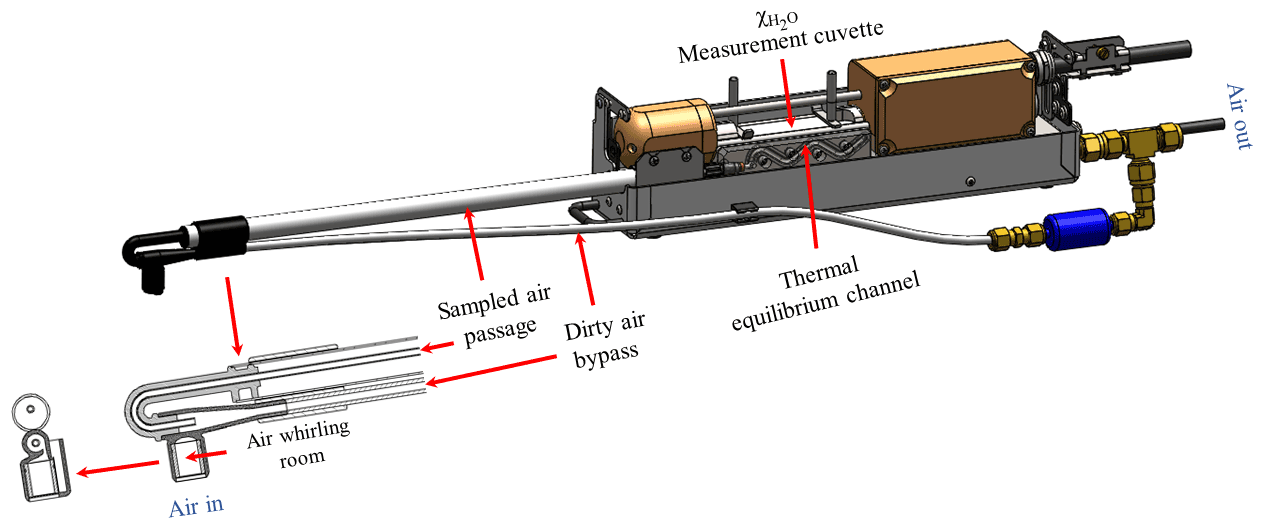
Figure 3 Vortex intake system for airflow through its individual compartments: air whirling room (2.200 mL), sampled air passage (1.889 mL), thermal equilibrium channel (0.587 mL), and ${\mathit{\chi }}_{{\mathrm{H}}_{\mathrm{2}}\mathrm{O}}$ measurement cuvette (5.887 mL). The internal space of all compartments adds up to a total volume of 10.563 mL.

Fortunately, the spatial separation scale is tens of centimeters, and the temporal lag scale is tens of milliseconds. In eddy-covariance flux measurements, such a separation misses some covariance signals at a higher frequency, which is correctable (Moore, 1986), and such a lag diminishes the covariance correlation, which is recoverable (Ibrom et al., 2007). How such a separation along with the lag influences the accuracy of Eq. (23), as shown in Fig. 2, needs testing against precision measurements of air temperature. The two advantages of the equation-computed T discussed in the Introduction, namely the fast response to high-frequency signals and the insensitivity to solar contamination in measurements, were studied and assessed during testing when a CPEC system was set up in the Campbell Scientific instrument test field (41.8^∘ N, 111.9^∘ W; 1360 m a.s.l.; UT, USA).

5 Materials and methods

5.1 Field test station

A CPEC310 system was set as the core of the station in 2018. Beyond its major components briefly described in Sect. 4, the system also included a barometer (model MPXAZ6115A, Freescale Semiconductor, TX, USA) for flow pressure; pump module (SN 1001) for air sampling; valve module (SN 1003) to control flows for auto-zero/span CO₂ and H₂O; scrub module (SN 1002) to generate zero air (i.e., without CO₂ and H₂O) for the auto-zero procedure; CO₂ cylinder for CO₂ span; and EC100 electronic module (SN 1002, OS Rev 07.01) to control and measure a CSAT3A, EC155, and barometer. In turn, the EC100 was connected to and instructed by a central CR6 datalogger (SN 2981, OS 04) for sensor measurements, data processing, and data output. In addition to receiving the data output from the EC100, the CR6 also controlled the pump, valve, and scrub modules and measured other micrometeorological sensors in support of this study.

The micrometeorological sensors included an LI-200 pyranometer (SN 18854, LI-COR Biosciences, NE, USA) to monitor incoming solar radiation, a precision platinum resistance temperature detector (RTD, model 41342, SN TS25360) inside a fan-aspirated radiation shield (model 43502, R.M. Young Company, MI, USA) to more accurately measure the T considered with minimized solar contamination due to higher fan-aspiration efficiency, and an HMP155A temperature and humidity sensor (SN 1073, Vaisala Corporation, Helsinki, Finland) inside a 14-plate wind-aspirated radiation shield (model 41005) to measure the T under conditions of potentially significant solar contamination during the day due to low wind-aspiration efficiency. The sensing centers of all sensors related to T_s, T, and RH were set at a height of 2.57 m above ground level. The land surface was covered by natural prairie with a grass height of 5 to 35 cm.

A CR6, supported by EasyFlux DL CR6CP (revised version for this study, Campbell Scientific Inc., UT, USA), controlled and sampled the EC100 at 20 Hz. For spectral analysis, the EC100 filtered the data of T_s and ${\mathit{\chi }}_{{\mathrm{H}}_{\mathrm{2}}\mathrm{O}}$ for anti-aliasing using a finite-impulse-response filter with a 0-to-10 Hz (Nyquist folding frequency) passing band (Saramäki, 1993). The EC155 was zeroed for CO₂–H₂O and spanned for CO₂ automatically every other day and spanned for H₂O monthly using an LI-610 Portable Dew Point Generator (LI-COR Biosciences, NE, USA). The LI-200, RTD, and HMP155A were sampled at 1 Hz because of their slow response and the fact that only their measurement means were of interest to this study.

The purpose of this station was to measure the eddy-covariance fluxes to determine turbulent transfers in the boundary-layer flows. The air temperature equation (i.e., Eq. 23) was developed for the T of the turbulent airflows sampled through the CPEC systems. Therefore, this equation can be tested based on how the CPEC310 measures the boundary-layer flows related to turbulent transfer.

5.2 Turbulent transfer and CPEC310 measurement

In atmospheric boundary-layer flows, air constituents along with heat and momentum (i.e., air properties) are transferred dominantly by individual turbulent flow eddies with various sizes (Kaimal and Finnigan, 1994). Any air property is considered to be more homogenous inside each smaller eddy and more heterogenous among larger eddies (Stull, 1988). Due to this heterogeneity, an eddy in motion among others transfers air properties to its surroundings. Therefore, to measure the transfer in amount and direction, a CPEC system was designed to capture T_s, ${\mathit{\chi }}_{{\mathrm{H}}_{\mathrm{2}}\mathrm{O}}$, and 3-D flow speeds from individual eddies. Ideal measurements, although impossible, would be fast enough to capture all eddies with different sizes through the measurement volume and sampling orifice of the CPEC system (Fig. 1). To capture more eddies of as many sizes as possible, the CPEC measurements were set at a high frequency (20 Hz in this study) because, given 3-D speeds, the smaller the eddy, the shorter time the said eddy takes to pass the sensor measurement volume. Ideally, each measurement captures an individual eddy for all variables of interest so that the measured values are representative of this eddy. So, for instance, in our effort to compute T from a pair of T_s and ${\mathit{\chi }}_{{\mathrm{H}}_{\mathrm{2}}\mathrm{O}}$ values, the pair simultaneously measured from the same eddy could better reflect its T at the measurement time; however, in a CPEC system, T_s and ${\mathit{\chi }}_{{\mathrm{H}}_{\mathrm{2}}\mathrm{O}}$ are measured with separation in both space (Fig. 1) and time (Fig. 3).

If an eddy passing the sonic anemometer is significantly larger than the dimension of separation between the T_s measurement volume and the ${\mathit{\chi }}_{{\mathrm{H}}_{\mathrm{2}}\mathrm{O}}$ sampling orifice (Fig. 1), the eddy is instantaneously measured for its 3-D wind and T_s in the volume while also sampled in the orifice for ${\mathit{\chi }}_{{\mathrm{H}}_{\mathrm{2}}\mathrm{O}}$ measurements. However, if the eddy is smaller and flows along the alignment of separation, the sampling takes place either a little earlier or a little later than the measurement (e.g., earlier if T_s is measured later, and vice versa). However, depending on its size, an eddy flowing beyond the alignment from other directions, although measured by the sonic anemometer, may be missed by the sampling orifice passed by other eddies and, in other cases, although sampled by the orifice, may be missed by the measurement of the sonic anemometer.

Additionally, the airflow sampled for ${\mathit{\chi }}_{{\mathrm{H}}_{\mathrm{2}}\mathrm{O}}$ measurements is not measured at its sampling time on the sampling orifice but instead is measured, in lag, inside the ${\mathit{\chi }}_{{\mathrm{H}}_{\mathrm{2}}\mathrm{O}}$ measurement cuvette (Fig. 3). The lag depends on the time needed for the sampled flow to travel through the CPEC sampling system (Fig. 3). Therefore, for the computation of $T,{\mathit{\chi }}_{{\mathrm{H}}_{\mathrm{2}}\mathrm{O}}$ is better synchronized and matched with T_s as if they were simultaneously measured from the same eddy.

5.3 Temporal synchronization and spatial match for T_s with ${\mathit{\chi }}_{{\mathrm{H}}_{\mathrm{2}}\mathrm{O}}$

In the CPEC310 system, a pair of T_s and ${\mathit{\chi }}_{{\mathrm{H}}_{\mathrm{2}}\mathrm{O}}$ values that were received by the CR6 from the EC100 in one data record (i.e., data row) were synchronously measured, through the Synchronous Device for Measurement communication protocol (Campbell Scientific Inc., 2018c), in the T_s measurement volume and ${\mathit{\chi }}_{{\mathrm{H}}_{\mathrm{2}}\mathrm{O}}$ measurement cuvette (Fig. 1). Accordingly, within one data row of time series received by the CR6, ${\mathit{\chi }}_{{\mathrm{H}}_{\mathrm{2}}\mathrm{O}}$ was sampled earlier than T_s was measured. As discussed above, T_s and ${\mathit{\chi }}_{{\mathrm{H}}_{\mathrm{2}}\mathrm{O}}$ in the same row, although measured at the same time, might not be measured from the same eddy. If so, the ${\mathit{\chi }}_{{\mathrm{H}}_{\mathrm{2}}\mathrm{O}}$ measurement from the same eddy of this T_s might occur in another data row, and vice versa. In any case, a logical procedure for a synchronized match is first to pair T_s with ${\mathit{\chi }}_{{\mathrm{H}}_{\mathrm{2}}\mathrm{O}}$ programmatically in the CR6, as the former was measured at the same time as the latter was sampled.

5.3.1 Synchronize T_s measured to ${\mathit{\chi }}_{{\mathrm{H}}_{\mathrm{2}}\mathrm{O}}$ sampled at the same time

Among the rows in time series received by the CR6, any two consecutive rows were measured sequentially at a fixed time interval (i.e., measurement interval). Accordingly, anemometer data in any data row can be synchronized with analyzer data in a later row from the eddy sampled by the analyzer sampling orifice at the measurement time of the sonic anemometer. How many rows later depends on the measurement interval and the time length of the analyzer sample from its sampling orifice to the measurement cuvette. The measurement interval commonly is 50 or 100 ms for a 20 or 10 Hz measurement frequency, respectively. The time length is determined by the internal space volume of the sampling system (Fig. 3) and the flow rate of sampled air driven by a diaphragm pump (Campbell Scientific Inc., 2018a).

As shown in Fig. 3, the total internal space is 10.563 mL. The rate of sampled air through the sampling system nominally is 6.0 L min⁻¹, at which the sampled air takes 106 ms to travel from the analyzer sampling orifice to the cuvette exhaust outlet (Fig. 3). Given that the internal optical volume inside the cuvette is 5.887 mL, the air in the cuvette was sampled during a period of 47 to 106 ms earlier. Accordingly, anemometer data in a current row of time series should be synchronized with analyzer data in the next row for 10 Hz data and, for 20 Hz data, in the row after that. After synchronization, the CR6 stores anemometer and analyzer data in a synchronized matrix (variables unrelated to this study were omitted) as a time series:

$$\begin{array}{}\text{(28)}& \left[\begin{array}{l}\mathrm{\cdots }\\ u\left(t_i\right)v\left(t_i\right)w\left(t_i\right)T_{\mathrm{s}}\left(t_i\right)d_{\mathrm{s}}\left(t_i\right){\mathit{\chi }}_{{\mathrm{H}}_{\mathrm{2}}\mathrm{O}}\left(t_i\right)d_{\mathrm{g}}\left(t_i\right)s\left(t_i\right)\\ \mathrm{\cdots }\end{array}\right],\end{array}$$

where u and v are horizontal wind speeds orthogonal to each other; w is vertical wind speed; d_s and d_g are diagnosis codes for the sonic anemometer and infrared analyzer, respectively; s is the analyzer signal strength for H₂O; t is time, and its subscript i is its index; and the difference between t_i and t_i+1 is a measurement interval ($\mathrm{\Delta }t=t_{i+\mathrm{1}}$ − t_i). In any row of the matrix (28) (e.g., the ith row), t_i for anemometer data is the measurement time plus instrument lag, and t_i for analyzer data is the sampling time plus the same lag. The instrument lag is defined as the number of measurement intervals used for data processing inside the EC100 after the measurement and subsequent data communication to the CR6. Regardless of instrument lag, T_s and ${\mathit{\chi }}_{{\mathrm{H}}_{\mathrm{2}}\mathrm{O}}$ in each row of the synchronization matrix were temporally synchronized as measured and sampled at the same time.

5.3.2 Match T_s measured to ${\mathit{\chi }}_{{\mathrm{H}}_{\mathrm{2}}\mathrm{O}}$ sampled from the same eddy

As discussed in Sect. 5.2, at either the T_s measurement or the ${\mathit{\chi }}_{{\mathrm{H}}_{\mathrm{2}}\mathrm{O}}$ sampling time, if an eddy is large enough to enclose both the T_s measurement volume and the ${\mathit{\chi }}_{{\mathrm{H}}_{\mathrm{2}}\mathrm{O}}$ sampling orifice (Fig. 1), T_s and ${\mathit{\chi }}_{{\mathrm{H}}_{\mathrm{2}}\mathrm{O}}$ in the same row of the synchronization matrix (28) belong to the same eddy; otherwise, they belong to different eddies. For any eddy size, it would be ideal if T_s could be spatially matched with ${\mathit{\chi }}_{{\mathrm{H}}_{\mathrm{2}}\mathrm{O}}$ as a pair for the same eddy; however, this match would not be possible for all T_s values simply because, in some cases, an eddy measured by the sonic anemometer might never be sampled by the ${\mathit{\chi }}_{{\mathrm{H}}_{\mathrm{2}}\mathrm{O}}$ sampling orifice, and vice versa (see Sect. 5.2). Realistically, T_s may be matched with ${\mathit{\chi }}_{{\mathrm{H}}_{\mathrm{2}}\mathrm{O}}$ overall with the most likelihood to as many pairs as possible for a period (e.g., an averaging interval).

The match will eventually lag either T_s or ${\mathit{\chi }}_{{\mathrm{H}}_{\mathrm{2}}\mathrm{O}}$, relatively, in the synchronization matrix (28). The lag can be counted as an integer number (l_s, where subscript s indicates the spatial separation causing lag) in measurement intervals, where l_s is positive if an eddy flowed through the T_s measurement volume earlier, negative if it flowed through later, or zero if it flowed through the ${\mathit{\chi }}_{{\mathrm{H}}_{\mathrm{2}}\mathrm{O}}$ sampling orifice at the same time. This number is estimated through the covariance maximization (Irwin, 1979; Moncrieff et al., 1997; Ibrom et al., 2007; Rebmann et al., 2012). According to l_s over an averaging interval, the data columns of the infrared analyzer over an averaging interval in the synchronization matrix (28) can be moved together up l_s rows as positive, down l_s rows as negative, or nowhere as zero to form a matched matrix:

$$\begin{array}{}\text{(29)}& \left[\begin{array}{l}\mathrm{\cdots }\\ u\left(t_i\right)v\left(t_i\right)w\left(t_i\right)T_{\mathrm{s}}\left(t_i\right)d_{\mathrm{s}}\left(t_i\right){\mathit{\chi }}_{{\mathrm{H}}_{\mathrm{2}}\mathrm{O}}\left(t_{i+l_{\mathrm{s}}}\right)d_{\mathrm{g}}\left(t_{i+l_{\mathrm{s}}}\right)s\left(t_{i+l_{\mathrm{s}}}\right)\\ \mathrm{\cdots }\end{array}\right].\end{array}$$

For details on how to find l_s, see EasyFlux DL CR6CP on https://www.campbellsci.com (last access: 11 December 2021). In the matched matrix (29), over an averaging interval, a pair of T_s and ${\mathit{\chi }}_{{\mathrm{H}}_{\mathrm{2}}\mathrm{O}}$ values in the same row can be assumed to be matched as if they were measured and sampled from the same eddy.

Using Eq. (23), the air temperature can now be computed using

$$\begin{array}{}\text{(30)}& T_{l_{\mathrm{s}}i}=T_{\mathrm{s}}\left(t_i\right){\displaystyle \frac{\left[\mathrm{1}+\mathit{\epsilon }{\mathit{\chi }}_{{\mathrm{H}}_{\mathrm{2}}\mathrm{O}}\left(t_{i+l_{\mathrm{s}}}\right)\right]\left[\mathrm{1}+\mathit{\epsilon }{\mathit{\gamma }}_{\mathrm{v}}{\mathit{\chi }}_{{\mathrm{H}}_{\mathrm{2}}\mathrm{O}}\left(t_{i+l_{\mathrm{s}}}\right)\right]}{\left[\mathrm{1}+{\mathit{\chi }}_{{\mathrm{H}}_{\mathrm{2}}\mathrm{O}}\left(t_{i+l_{\mathrm{s}}}\right)\right]\left[\mathrm{1}+\mathit{\epsilon }{\mathit{\gamma }}_{\mathrm{p}}{\mathit{\chi }}_{{\mathrm{H}}_{\mathrm{2}}\mathrm{O}}\left(t_{i+l_{\mathrm{s}}}\right)\right]}},\end{array}$$

where subscript l_s for t indicates that spatially lagged ${\mathit{\chi }}_{{\mathrm{H}}_{\mathrm{2}}\mathrm{O}}$ is used for computation of T. In verification of the accuracy of equation-computed T and in assessments of its expected advantages of high-frequency signals insensitive to solar contamination in measurements, $T_{l_{\mathrm{s}}i}$ could minimize the uncertainties due to the spatial separation in measurements of T_s and ${\mathit{\chi }}_{{\mathrm{H}}_{\mathrm{2}}\mathrm{O}}$ between the T_s measurement volume and the ${\mathit{\chi }}_{{\mathrm{H}}_{\mathrm{2}}\mathrm{O}}$ sampling orifice (Fig. 1).

6 Results

6.1 Verification of the accuracy of equation-computed T

The accuracy of equation-computed T was theoretically specified by Eqs. (25) to (27) and was estimated in Fig. 2c. This accuracy specifies the range of equation-computed T minus true T (i.e., ΔT). However, true T was not available in the field, but, as usual, precision measurements could be considered benchmarks to represent true T. In this study, T measured by the RTD inside a fan-aspirated radiation shield (T_RTD) was the benchmark to compute ΔT (i.e., equation-computed T minus T_RTD). If almost all ΔT values fall within the accuracy-specified range over a measurement domain of T and ${\mathit{\chi }}_{{\mathrm{H}}_{\mathrm{2}}\mathrm{O}}$, the accuracy is correctly defined, and the equation-computed T is accurate as specified.

To verify that the accuracy over the domain is as large as possible, ΔT values in the coldest (January) and hottest (July) months were used as shown in Fig. 4 (−21 ^∘C < T < 35.5 ^∘C, and ${\mathit{\chi }}_{{\mathrm{H}}_{\mathrm{2}}\mathrm{O}}$ up to 20.78 mmolH₂O mol⁻¹ in a 30 min mean over both months). Out of 2976 ΔT values from both months, 44 values fell out of the specified accuracy range but were near the range line within 0.30 K. The ΔT values were 0.549 ± 0.281 K in January and 0.436 ± 0.290 K in July. Although these values were almost all positively away from the zero line due to either overestimation for T_s by the sonic anemometer within ±1.00 K accuracy or underestimation for T_RTD by the RTD within ±0.20 K accuracy, the ranges are significantly narrower than the specified accuracy range of equation-computed T (Figs. 2c and 4).

It is common for sonic anemometers to have a systematic error in T_s of ±0.5 ^∘C or a little greater, which is the reason that the T_s accuracy is specified by Larry Jacobsen (anemometer authority) to be ±1.0 ^∘C for the updated CSAT3A. The fixed deviation in measurements of sonic path lengths is asserted as a source of bias in T_s (Zhou et al., 2018). This bias brings an error to equation-computed T. If the T equation were not exact as in Eqs. (4) and (5), there would be an additional equation error. In our study effort, this bias from fixed deviation is possibly around 0.5 ^∘C. With this bias, the equation-computed T is still accurate, as specified by Eqs. (25) to (27), and even better.

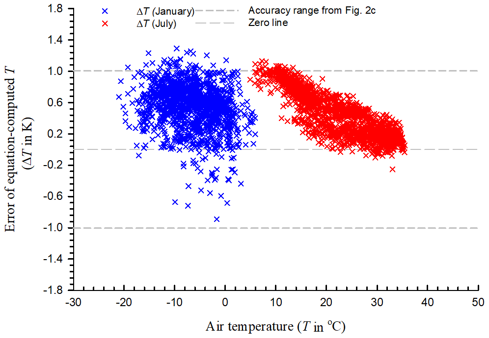
Figure 4 The error in equation-computed T in the coldest (January) and hottest (July) months of 2019 in Logan, UT, USA. ΔT is equation-computed T minus RTD-measured T, where RTD denotes a precision platinum resistance temperature detector inside a fan-aspirated radiation shield. ΔT is 0.549 ± 0.281 K in January and 0.436 ± 0.290 K in July. See Fig. 2c for the accuracy range.

6.2 Assessments of the advantages of equation-computed T

As previously discussed, the data stream of equation-computed T consists of high-frequency signals insensitive to solar contamination in measurements. Its frequency response can be assessed against known high-frequency signals of T_s, and the insensitivity can be assessed by analyzing the equation-computed, RTD-measured, and sensor-measured T, where the sensor is an HMP155A inside a wind-aspirated radiation shield.

6.2.1 Frequency response

The matched matrix (29) and Eq. (30) were used to compute $T_{l_{\mathrm{s}}i}$ (i.e., equation-computed T). Paired power spectra of equation-computed T and T_s are compared in Fig. 5 for three individual 2 h periods of atmospheric stratifications, including unstable ($z/L$ is −0.313 to −2.999, where z is a dynamic height of measurement minus displacement height and L is the Monin–Obukhov length), near-neutral ($z/L$ is −0.029 to +0.003), and stable ($z/L$ is +0.166 to +0.600). Slower response of equation-computed T than T_s at a higher frequency (e.g., > 5 Hz) was expected because equation-computed T is derived from two variables (T_s and ${\mathit{\chi }}_{{\mathrm{H}}_{\mathrm{2}}\mathrm{O}}$) measured in a spatial separation, which attenuates the frequency response of correlation of two measured variables (Laubach and McNaughton, 1998), and ${\mathit{\chi }}_{{\mathrm{H}}_{\mathrm{2}}\mathrm{O}}$ from a CPEC system has a slower response than T_s in terms of frequency (Ibrom et al., 2007). However, the expected slower response was not found in this study. In unstable and stable atmospheric stratifications (Fig. 5a and c), each pair of power spectra almost overlaps. Although they do not overlap in the near-neutral atmospheric stratification (Fig. 5b), the pairs follow the same trend slightly above or below one another. In the higher-frequency band of 1 to 10 Hz in Fig. 5a and b, equation-computed T has a little more power than T_s. The three pairs of power spectra in Fig. 5 indicate that equation-computed T has a frequency response equivalent to T_s up to 10 Hz, with a 20 Hz measurement rate considered to be a high frequency. The equivalent response might be accounted for by a dominant role of T_s in the magnitude of equation-computed T.

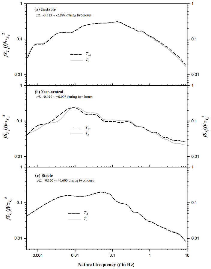
Figure 5 Paired comparisons of power spectra for equation-computed air temperature (T) and sonic temperature (T_s) at each of three atmospheric stratifications: unstable (a), near-neutral (b), and stable (c). T₊₁ and T₋₃ are equation-computed T from T_s and the H₂O mixing ratio of air sampled by the CPEC system through its sampling orifice in +1 lag (50 ms behind) and in −3 lags (150 ms ahead) of T_s measurement; z is the dynamic height of measurement minus the displacement height; L is the Monin–Obukhov length; $S_{T_{\mathrm{s}}}\left(f\right)$, $S_{T_{+\mathrm{1}}}\left(f\right)$, and $S_{T_{-\mathrm{3}}}\left(f\right)$ are the power spectra of T_s, T₊₁, and T₋₃ at f; and ${\mathit{\sigma }}_{T_{\mathrm{s}}}^{\mathrm{2}}$, ${\mathit{\sigma }}_{T_{+\mathrm{1}}}^{\mathrm{2}}$, and ${\mathit{\sigma }}_{T_{-\mathrm{3}}}^{\mathrm{2}}$ represent the variance of T_s, T₊₁, and T₋₃.

6.2.2 Insensitivity to solar contamination in measurements

The data of equation-computed, sensor-measured, and RTD-measured T in July, during which incoming solar radiation (R_s) at the site was strongest in a yearly cycle, are used to assess the insensitivity of equation-computed T. From the data, ΔT is considered to be an error in equation-computed T. The error in sensor-measured T can be defined as sensor-measured T minus RTD-measured T, denoted by ΔT_m. From Fig. 6, ΔT (0.690 ± 0.191 K) is > ΔT_m (0.037 ± 0.199 K) when R_s < 50 W m⁻² at lower radiation. However, ΔT (0.234 ± 0.172 K) is < ΔT_m (0.438 ± 0.207 K) when R_s>50 W m⁻² at higher radiation. This difference between ΔT and ΔT_m shows a different effect of R_s on equation-computed and sensor-measured T.

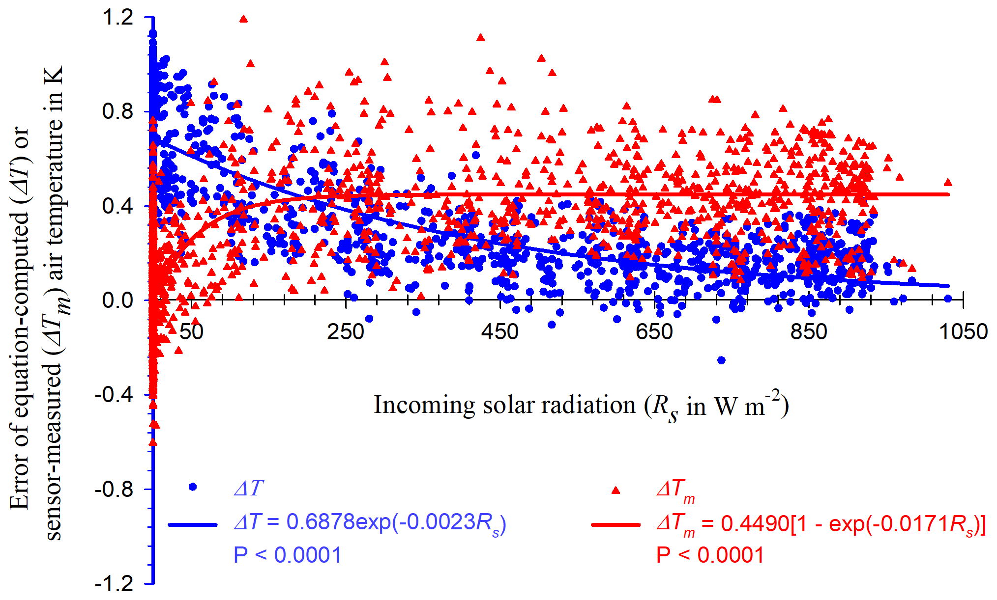
Figure 6 Errors in equation-computed and sensor-measured air temperature (T) with incoming solar radiation. ΔT is equation-computed T minus RTD-measured T, where RTD denotes a precision platinum resistance temperature detector inside a fan-aspirated radiation shield. ΔT_m is sensor-measured T minus RTD-measured T, where the sensor is an HMP155A air temperature and humidity probe inside a wind-aspirated radiation shield.

As shown in Fig. 6, ΔT_m increases sharply with increasing R_s for R_s<250 W m⁻², beyond which it asymptotically approaches 0.40 K. In the range of lower R_s, atmospheric stratification was likely stable (Kaimal and Finnigan, 1994), under which the heat exchange by wind was ineffective between the wind-aspirated radiation shield and boundary-layer flows. In this case, sensor-measured T was expected to increase with R_s increase (Lin et al., 2001; Blonquist and Bugbee, 2018). Along with R_s increase, the atmospheric boundary layer develops from stable to neutral or unstable conditions (Kaimal and Finnigan, 1994). During the stability change, the exchange becomes increasingly more effective, offsetting the further heating from R_s increase on the wind-aspirated radiation shield as indicated by the red asymptote portion in Fig. 6. Compared to the ΔT_m mean (0.037 K) while R_s<50 W m⁻², the magnitude of the asymptote above the mean is the overestimation of sensor-measured T due to solar contamination.

However, ΔT decreases asymptotically from about 0.70 K toward zero with the increase in R_s from 50 to 250 W m⁻² and beyond, with a more gradual rate of change than ΔT_m at the lower radiation range. Lower R_s (e.g., < 250 W m⁻²) concurrently occurs with lower T, higher RH, and/or unfavorable weather to T_s measurements. Under lower T (e.g., below 20 ^∘C of normal CSAT3A manufacturing conditions), the sonic path lengths of CSAT3A (Fig. 1) must become, due to thermo-contraction of sonic anemometer structure, shorter than those at 20 ^∘C. As a result, the sonic anemometer could overestimate the speed of sound (Zhou et al., 2018) and, hence, T_s for equation-computed T, resulting in greater ΔT with lower R_s. Under higher RH conditions, dew may form on the sensing surface of the six CSAT3A sonic transducers (Fig. 1). The dew, along with unfavorable weather, could contaminate the T_s measurements, resulting in ΔT greater in magnitude. Higher R_s (e.g., > 250 W m⁻²) concurrently occurs with weather favorable to T_s measurements, which is the reason that ΔT slightly decreases rather than increases with R_s when R_s > 250 W m⁻².

Again from Fig. 6, the data pattern of ΔT>ΔT_m in the lower R_s range and ΔT<ΔT_m in the higher R_s range shows that equation-computed T is not as sensitive to R_s as sensor-measured T. The decreasing trend of ΔT with R_s increase shows the insensitivity of equation-computed T to R_s. Although the purpose of this study is not particularly to eliminate solar radiation contamination, equation-computed T is indeed less contaminated by solar radiation, as shown in Fig. 6.

7 Discussion

7.1 Actual accuracy

The range of ΔT curves for each RH level in Fig. 2 is the maximum at that level because the data were evaluated using the maximized measurement uncertainties from all sources. Accordingly, in field applications under weather favorable to T_s measurements, the range of actual accuracy in equation-computed T can be reasonably inferred to be narrower. In our study case as shown in Figs. 4 and 6, the variability in ΔT was narrower than the accuracy range as specified in Fig. 2. In other words, the actual accuracy is better.

However, under weather conditions unfavorable to T_s measurements, such as dew, rain, snow, or dust storms, the accuracy of T_s measurements cannot be easily evaluated. T_s measurements also possibly have a systematic error due to the fixed deviation in the measurements of sonic path lengths for sonic anemometers, although the error should be within the accuracy specified in Fig. 2. A ${\mathit{\chi }}_{{\mathrm{H}}_{\mathrm{2}}\mathrm{O}}$ measurement can also be erroneous if the infrared analyzer is not periodically zeroed and spanned for its measurement environment. Therefore, if T_s is measured under unfavorable weather conditions and the sonic anemometer produces a systematic T_s error and if the infrared analyzer is not zeroed and spanned as instructed in its manual, then the accuracy of equation-computed T would be unpredictable. Normally, the actual accuracy is better than that specified in Fig. 2. Additionally, with the improvement in measurement accuracies of sonic anemometers (e.g., weather-condition-regulated, heated, 3-D sonic anemometers; Mahan et al., 2021) and infrared analyzers, this accuracy of equation-computed T would gradually become better.

For this study, filtering out the T_s data in the periods of unfavorable weather could narrow the error range of equation-computed T. The unfavorable weather was suspected of contributing to the stated error. However, although filtering out unfavorable weather cases could create a lower error estimate, most field experiments include periods when weather increases a T_s error, so including a weather contribution to error would prevent overstating instrument accuracy under typical (unfiltered) applications. Therefore, both T_s and ${\mathit{\chi }}_{{\mathrm{H}}_{\mathrm{2}}\mathrm{O}}$ data in this study were not programmatically or manually filtered based on weather.

7.2 Spatial separation of T_s and ${\mathit{\chi }}_{{\mathrm{H}}_{\mathrm{2}}\mathrm{O}}$ in measurements

In this study, T was successfully computed from T_s and ${\mathit{\chi }}_{{\mathrm{H}}_{\mathrm{2}}\mathrm{O}}$ as a high-frequency signal (Fig. 5) with expected accuracy as tested in Figs. 2, 4, and 6, where both were measured separately from two sensors in a spatial separation. Some open-path eddy-covariance (OPEC) flux systems (e.g., CSAT3A + EC150 and CSAT3B + LI-7500) measure T_s and ρ_w also using two sensors in a spatial separation. To OPEC systems, although the air temperature equation (Eq. 23) is not applicable, the algorithms developed in Sect. 5.3 to temporally synchronize and spatially match T_s with ${\mathit{\chi }}_{{\mathrm{H}}_{\mathrm{2}}\mathrm{O}}$ for computation of T are applicable for computation of T from T_s and ρ_w along with P in such OPEC systems (Swiatek, 2018).

In Sect. 5.3, programming and computing are needed to pair T_s measured to ${\mathit{\chi }}_{{\mathrm{H}}_{\mathrm{2}}\mathrm{O}}$ sampled at the same time into the synchronization matrix (28) as the first step and from the same eddy into matched matrix (29) as the second step. The second requires complicated programming and much computing. To test the necessity of this step in specific cases, using Eq. (30), T_0i was computed from a row of the synchronization matrix, and $T_{l_{\mathrm{s}}i}$ was computed from this matrix by lagging ${\mathit{\chi }}_{{\mathrm{H}}_{\mathrm{2}}\mathrm{O}}$ columns up l_s rows if l_s>0 and down $\left|l_{\mathrm{s}}\right|$ rows if l_s<0, where l_s is $-\mathrm{5},\mathrm{\dots },-$1 and $+\mathrm{1},\mathrm{\dots },+$5. From the data of this study, individual $T_{l_{\mathrm{s}}i}$ values were different for different subscript l_s values, but their means for subscript i over an averaging interval $\left(T_{l_{\mathrm{s}}}\right)$ are the same to at least the fourth digit after the decimal place. Further, the power spectrum of T_0i time series was compared to those of $T_{l_{\mathrm{s}}i}$ time series, where l_s≠0. Any pair of power spectra from the same period overlaps exactly (figures omitted). Therefore, the second step of lag maximization to match T_s measured to ${\mathit{\chi }}_{{\mathrm{H}}_{\mathrm{2}}\mathrm{O}}$ sampled from the same eddy is not needed if only the hourly mean and power spectrum of equation-computed T are of interest to computations, for both CPEC and OPEC systems.

7.3 Applications

The air temperature equation (Eq. 23) is derived from first principles without any assumption and approximation. It is an exact equation from which T can be computed in CPEC systems as a high-frequency signal insensitive to solar radiation. These merits, in additional to its consistent representation of spatial measurement and temporal synchronization scales with other thermodynamic variables for boundary-layer turbulent flows, will be particularly needed for advanced applications. The EasyFlux series is one of the two most popular field eddy-covariance flux software packages used in the world, the other being EddyPro (LI-COR Biosciences, 2015). Currently, it has used equation-computed T for ρ_d in Eq. (1), sensible heat flux (H), and RH as a high-frequency signal in CPEC systems (Campbell Scientific Inc., 2018a).

7.3.1 Dry-air density

As a high-frequency signal insensitive to solar radiation, equation-computed T is more applicable than sensor-measured T for calculations of ${\overline{\mathit{\rho }}}_{\mathrm{d}}$ and $\stackrel{\mathrm{‾}}{{\mathit{\rho }}_{\mathrm{d}}w}$ for advanced applications (Gu et al., 2012; Foken et al., 2012). In practice, equation-computed T can surely be used for ${\overline{\mathit{\rho }}}_{\mathrm{d}}$ and $\stackrel{\mathrm{‾}}{{\mathit{\rho }}_{\mathrm{d}}w}$ under normal weather conditions while the sonic anemometer and infrared analyzer are normally running, which can be judged by their diagnosis codes (Campbell Scientific Inc., 2018a). Under a weather condition unfavorable to T_s measurements, such as dew, rain, snow, and/or ice, equation-computed T from weather-condition-regulated, heated, 3-D sonic anemometers (Mahan et al., 2021) and infrared analyzers could be an alternative.

Currently, in CO₂, H₂O, and trace gas flux measurements, ${\overline{\mathit{\rho }}}_{\mathrm{d}}$ for flux calculations is estimated from T and RH along with P. T and RH are measured mostly by a slow-response T–RH probe without fan aspiration (e.g., HMP155A; Zhu et al., 2021). As shown in Fig. 6, equation-computed T is better than probe-measured T. The air moisture measured by an infrared analyzer in CPEC systems must be more accurate (Eq. 27 and Fig. 2b) than probe-measured air moisture. The better equation-computed T along with more accurate air moisture has no reason not to improve the estimation for ${\overline{\mathit{\rho }}}_{\mathrm{d}}$.

7.3.2 Sensible heat flux estimated from a CPEC system

Currently, beyond the EasyFlux DL CR6CP series, H is derived from $\stackrel{\mathrm{‾}}{T_{\mathrm{s}}^{\prime }{w}^{\prime }}$ with a humidity correction (van Dijk, 2002). The correction equations were derived by Schotanus et al. (1983) and van Dijk (2002) in two ways, but both were derived with the approximation from Eq. (4) (see Appendix A). Using the exact equation from this study, theoretically H can be more accurately estimated directly from $\stackrel{\mathrm{‾}}{T^{\prime }{w}^{\prime }}$, where T is the equation-computed air temperature, although more studies and tests for this potential application are needed. Without our exact T equation, in any flux software, either Eq. (4) or Eq. (5) must be used for H computation. Both equations are approximate (see Appendices A and B). Compared to either, our exact equation must be an improvement on the mathematical representation of H. If the equation for sensible heat flux is approximate, then even a perfect measurement gives only an approximate value for the flux.

7.3.3 RH as a high-frequency signal

Conventionally, RH is measured using a T–RH probe, which is unable to track the high-frequency fluctuations in RH. In a CPEC system, equation-computed T, analyzer-measured ${\mathit{\chi }}_{{\mathrm{H}}_{\mathrm{2}}\mathrm{O}}$, and transducer-measured P are able to catch the fluctuations in these variables at a high frequency, from which RH can be computed (Sonntag, 1990; also see Appendix C). This method should provide high-frequency RH, although verification for a frequency response is needed. Currently, the applications of high-frequency properties in this RH are unknown in a CPEC system. Regardless, equation-computed T provides a potential opportunity to acquire the high-frequency RH for its application in the future.

8 Concluding remarks

In a CPEC flux system, the air temperature (T) of boundary-layer flows through the space of sonic anemometer measurement and infrared analyzer sampling (Fig. 1) is desired for a high frequency (e.g., 10 Hz) with consistent representation of spatial and temporal scales for moist turbulence thermodynamics characterized by three-dimensional wind from the sonic anemometer and H₂O–CO₂ and atmospheric pressure from the infrared analyzer. High-frequency T in the space can be measured using fine-wire thermocouples, but this kind of thermocouple for such an application is not durable under adverse climate conditions, being easily contaminated by solar radiation (Campbell, 1969). Nevertheless, the measurements of sonic temperature (T_s) and H₂O inside a CPEC system are high-frequency signals. Therefore, high-frequency T can be reasonably expected when computed from T_s and H₂O-related variables. For this expectation, two equations (i.e., Eqs. 4 and 5) are currently available. In both equations, converting H₂O-related variables into H₂O mixing ratios analytically reveals the difference between the two equations. This difference in CPEC systems reaches ±0.18 K, bringing an uncertainty into the accuracy of T from either equation and raising the question of which equation is better. To clarify the uncertainty and answer this question, the air temperature equations in terms of T_s and H₂O-related variables are thoroughly reviewed (Sects. 2 and 3, Appendices A and B). The two currently used equations (i.e., Eqs. 4 and 5) were developed and completed with approximations (Appendices A and B). Because of the approximations, neither of their accuracies was evaluated, nor was the question answered.

Using the first-principles equations, the air temperature equation in terms of T_s and ${\mathit{\chi }}_{{\mathrm{H}}_{\mathrm{2}}\mathrm{O}}$ (H₂O molar mixing ratio) is derived without any assumption and approximation (Eq. 23); therefore, the equation derived in this study does not itself have any error, and, as such, the accuracy in equation-computed T depends solely on the measurement accuracies of T_s and ${\mathit{\chi }}_{{\mathrm{H}}_{\mathrm{2}}\mathrm{O}}$. Based on the specifications for T_s and ${\mathit{\chi }}_{{\mathrm{H}}_{\mathrm{2}}\mathrm{O}}$ in the CPEC300 series, the accuracy of equation-computed T over the T_s and ${\mathit{\chi }}_{{\mathrm{H}}_{\mathrm{2}}\mathrm{O}}$ measurement ranges can be specified within ±1.01 K (Fig. 2). This accuracy range is propagated mainly (±1.00 K) from the uncertainty in T_s measurements (Fig. 2a) and a little (±0.02 K) from the uncertainty in ${\mathit{\chi }}_{{\mathrm{H}}_{\mathrm{2}}\mathrm{O}}$ measurements (Fig. 2b).

Under normal sensor and weather conditions, the specified accuracy is verified based on field data as valid, and actual accuracy is better (Figs. 4 and 6). Field data demonstrate that equation-computed T values under unstable, near-neutral, and stable atmospheric stratifications all have frequency responses equivalent to high-frequency T_s up to 10 Hz at a 20 Hz measurement rate (Fig. 5), being insensitive to solar contamination in measurements (Fig. 6).

The current applications of equation-computed T in a CPEC system are to calculate dry-air density (ρ_d) for the estimations of CO₂ flux (${\overline{\mathit{\rho }}}_{\mathrm{d}}\stackrel{\mathrm{‾}}{{\mathit{\chi }}_{{\mathrm{CO}}_{\mathrm{2}}}^{\prime }{w}^{\prime }}$, where ${\mathit{\chi }}_{{\mathrm{CO}}_{\mathrm{2}}}$ is the CO₂ mixing ratio, w is vertical velocity of air, the prime indicates the fluctuation of the variable away from its mean, and the overbar implies the mean), H₂O flux (${\overline{\mathit{\rho }}}_{\mathrm{d}}\stackrel{\mathrm{‾}}{{\mathit{\chi }}_{{\mathrm{H}}_{\mathrm{2}}\mathrm{O}}^{\prime }{w}^{\prime }}$), and other fluxes. Combined with measurements of ${\mathit{\chi }}_{{\mathrm{H}}_{\mathrm{2}}\mathrm{O}}$, 3-D wind speeds, and P, the equation-computed T can be applied to the estimation of ${\overline{\mathit{\rho }}}_{\mathrm{d}}$ and $\stackrel{\mathrm{‾}}{{\mathit{\rho }}_{\mathrm{d}}w}$ if needed (Gu et al., 2012; Foken et al., 2012), to the computation of high-frequency RH (Sonntag, 1990), and to the derivation of sensible heat flux (H) avoiding the humidity correction as needed for H indirectly from T_s (Schotanus et al., 1983; van Dijk, 2002).

In a CPEC flux system, although T_s and ${\mathit{\chi }}_{{\mathrm{H}}_{\mathrm{2}}\mathrm{O}}$ are measured using two spatially separated sensors of a sonic anemometer and infrared analyzer, T was successfully computed from both measured variables as a high-frequency signal (Fig. 5) with an expected accuracy (Figs. 2 and 4). Some open-path eddy-covariance (OPEC) flux systems measure T_s and water vapor density (ρ_w) also using two sensors in a similar way. The algorithms developed in Sect. 5.3 to temporally synchronize and spatially match T_s with ${\mathit{\chi }}_{{\mathrm{H}}_{\mathrm{2}}\mathrm{O}}$ for computation of T are applicable to such OPEC systems to compute T from T_s and ρ_w along with P. This T would be a better option than sensor-measured T in the systems for the correction of the spectroscopic effect in measuring CO₂ fluctuations at high frequencies (Helbig et al., 2016; Wang et al., 2016). With the improvements in measurement technologies for T_s and ${\mathit{\chi }}_{{\mathrm{H}}_{\mathrm{2}}\mathrm{O}}$, particularly for T_s, the T from our developed equation will become increasingly more accurate. Having its accuracy combined with its high frequency, this T with consistent representation of all other thermodynamic variables for moist air at the spatial and temporal scales in CPEC measurements has its advanced merits in boundary-layer meteorology and applied meteorology.

Appendix A: Derivation of Eq. (4)

The sonic temperature (T_s) reported by a three-dimensional sonic anemometer is internally calculated from its measurements of the speed of sound in moist air (c) after the crosswind correction (Zhou et al., 2018), using

$$\begin{array}{}\text{(A1)}& T_{\mathrm{s}}={\displaystyle \frac{c^{\mathrm{2}}}{{\mathit{\gamma }}_{\mathrm{d}}{R}_{\mathrm{d}}}},\end{array}$$

where subscript d indicates dry air, γ_d is the specific heat ratio of dry air between constant pressure and constant volume, and R_d is the gas constant for dry air (Campbell Scientific Inc., 2018b). The speed of sound in the atmospheric boundary layer as in a homogeneous gaseous medium is well defined in acoustics (Barrett and Suomi, 1949), given by

$$\begin{array}{}\text{(A2)}& c^{\mathrm{2}}=\mathit{\gamma }{\displaystyle \frac{P}{\mathit{\rho }}},\end{array}$$

where γ is the counterpart of γ_d for moist air, P is atmospheric pressure, and ρ is moist-air density. These variables are related to air temperature and air specific humidity (q, i.e., the mass ratio of water vapor to moist air).

A1 Moist-air density (ρ)

Moist-air density is the sum of dry-air and water vapor densities. Based on the ideal gas law (Wallace and Hobbs, 2006), dry-air density (ρ_d) is given by

$$\begin{array}{}\text{(A3)}& {\mathit{\rho }}_{\mathrm{d}}={\displaystyle \frac{P-e}{R_{\mathrm{d}}T}},\end{array}$$

where e is water vapor pressure, and the water vapor density (ρ_w) is given by

$$\begin{array}{}\text{(A4)}& {\mathit{\rho }}_{\mathrm{w}}={\displaystyle \frac{e}{R_{\mathrm{v}}T}},\end{array}$$

where R_v is the gas constant for water vapor. Therefore, moist-air density in Eq. (A2) can be expressed as

$$\begin{array}{}\text{(A5)}& \mathit{\rho }={\displaystyle \frac{P-e}{R_{\mathrm{d}}T}}+{\displaystyle \frac{e}{R_{\mathrm{v}}T}}.\end{array}$$

Because $R_{\mathrm{d}}/R_{\mathrm{v}}=\mathit{\epsilon }$ (i.e., 0.622, the molar mass ratio between water vapor and dry air), this equation can be rearranged as

$$\begin{array}{}\text{(A6)}& \mathit{\rho }={\displaystyle \frac{P}{R_{\mathrm{d}}T}}\left[\mathrm{1}-\left(\mathrm{1}-\mathit{\epsilon }\right){\displaystyle \frac{e}{P}}\right].\end{array}$$

Using Eqs. (A4) and (A6), the air specific humidity can be expressed as

$$\begin{array}{}\text{(A7)}& q\equiv {\displaystyle \frac{{\mathit{\rho }}_{\mathrm{w}}}{\mathit{\rho }}}={\displaystyle \frac{\mathit{\epsilon }e}{P-(\mathrm{1}-\mathit{\epsilon })e}}.\end{array}$$

Because $P\gg (\mathrm{1}-\mathit{\epsilon })e$, q can be approximated as

$$\begin{array}{}\text{(A8)}& q\approx \mathit{\epsilon }{\displaystyle \frac{e}{P}}.\end{array}$$

Substituting this relation into Eq. (A6) generates

$$\begin{array}{}\text{(A9)}& \mathit{\rho }={\displaystyle \frac{P}{R_{\mathrm{d}}T}}\left(\mathrm{1}-{\displaystyle \frac{\mathrm{1}-\mathit{\epsilon }}{\mathit{\epsilon }}}q\right).\end{array}$$

A2 Specific heat ratio of moist air (γ)

The specific heat ratio of moist air is determined by two moist-air properties: (1) the specific heat at constant pressure (C_p) and (2) specific heat at constant volume (C_v). C_p varies with the air moisture content between the specific heat of dry air at constant pressure (C_pd) and the specific heat of water vapor at constant pressure (C_pw). It must be the average of C_pd and C_pw that is arithmetically weighted by the dry air mass and water vapor mass, respectively, given by (Stull, 1988)

$$\begin{array}{}\text{(A10)}& C_{\mathrm{p}}={\displaystyle \frac{C_{\mathrm{pd}}{\mathit{\rho }}_{\mathrm{d}}+C_{\mathrm{pw}}{\mathit{\rho }}_{\mathrm{w}}}{\mathit{\rho }}}.\end{array}$$

C_v can be similarly determined:

$$\begin{array}{}\text{(A11)}& C_{\mathrm{v}}={\displaystyle \frac{C_{\mathrm{vd}}{\mathit{\rho }}_{\mathrm{d}}+C_{\mathrm{vw}}{\mathit{\rho }}_{\mathrm{w}}}{\mathit{\rho }}},\end{array}$$

where C_vd is the specific heat of dry air at constant volume and C_vw is the specific heat of water vapor at constant volume. Denoting $C_{\mathrm{pd}}/C_{\mathrm{vd}}$ as γ_d, Eqs. (A10) and (A11) are used to express γ as

$$\begin{array}{}\text{(A12)}& \mathit{\gamma }={\displaystyle \frac{C_{\mathrm{p}}}{C_{\mathrm{v}}}}={\mathit{\gamma }}_{\mathrm{d}}{\displaystyle \frac{(\mathrm{1}-q)+q{C}_{\mathrm{pw}}/C_{\mathrm{pd}}}{(\mathrm{1}-q)+q{C}_{\mathrm{vw}}/C_{\mathrm{vd}}}}.\end{array}$$

A3 Relation of sonic temperature to air temperature

Substituting Eqs. (A9) and (A12) into Eq. (A2) leads to

$$\begin{array}{}\text{(A13)}& c^{\mathrm{2}}={\mathit{\gamma }}_{\mathrm{d}}{R}_{\mathrm{d}}T{\displaystyle \frac{(\mathrm{1}-q)+q{C}_{\mathrm{pw}}/C_{\mathrm{pd}}}{\left[(\mathrm{1}-q)+q{C}_{\mathrm{vw}}/C_{\mathrm{vd}}\right]\left(\mathrm{1}-\frac{\mathrm{1}-\mathit{\epsilon }}{\mathit{\epsilon }}q\right)}}.\end{array}$$

Using this equation to replace c² in Eq. (A1), T_s is expressed as

$$\begin{array}{}\text{(A14)}& T_{\mathrm{s}}=T{\displaystyle \frac{(\mathrm{1}-q)+q{C}_{\mathrm{pw}}/C_{\mathrm{pd}}}{\left[(\mathrm{1}-q)+q{C}_{\mathrm{vw}}/C_{\mathrm{vd}}\right]\left(\mathrm{1}-\frac{\mathrm{1}-\mathit{\epsilon }}{\mathit{\epsilon }}q\right)}}.\end{array}$$

Given C_pw=1952, C_pd=1004, C_vw=1463, and C_vd=717 J K⁻¹ kg⁻¹ (Wallace and Hobbs, 2006), this equation becomes

$$\begin{array}{}\text{(A15)}& \begin{array}{rl}{T}_{\mathrm{s}}=& T\left(\mathrm{1}+\mathrm{0.944223}q\right)\left({\displaystyle \frac{\mathrm{1}}{\mathrm{1}+\mathrm{1.040446}q}}\right)\\ & \left({\displaystyle \frac{\mathrm{1}}{\mathrm{1}-\mathrm{0.607717}q}}\right).\end{array}\end{array}$$

Expression of the last two parenthesized terms on the right side of this equation separately as Taylor series of q (Burden and Faires, 1993) by dropping, due to q≪1, the second-or-higher-order terms related to q leads to

$$\begin{array}{}\text{(A16)}& \begin{array}{rl}{T}_{\mathrm{s}}\approx & T\left(\mathrm{1}+\mathrm{0.944223}q\right)\left(\mathrm{1}-\mathrm{1.040446}q\right)\\ & \left(\mathrm{1}+\mathrm{0.607717}q\right).\end{array}\end{array}$$

On the right side of this equation, the three parenthesized terms can be expanded into a polynomial of q of the third order. Also due to q≪1 in this polynomial, the terms of q of the second or third order can be dropped. Further arithmetical manipulations result in

$$\begin{array}{}\text{(A17)}& T_{\mathrm{s}}\approx T\left(\mathrm{1}+\mathrm{0.51}q\right).\end{array}$$

This is Eq. (4) in a different form. In its derivations from Eqs. (A1) and (A2), three approximation procedures were used from Eqs. (A7) to (A8), (A15) to (A16), and (A16) to (A17). The three approximations must bring unspecified errors into the derived equation.

Appendix B: Derivation of Eq. (5)

Equation (5) was sourced from Ishii (1935) in which the speed of sound in moist air (c) was expressed in his Eq. (1) as

$$\begin{array}{}\text{(B1)}& c^{\mathrm{2}}=\mathit{\gamma }\left({\displaystyle \frac{P}{\mathit{\rho }}}\right)\left({\displaystyle \frac{\mathit{\alpha }}{\mathit{\beta }}}\right),\end{array}$$

where all variables in this equation are for moist air, γ is the specific heat ratio of moist air between constant pressure and constant volume, P is moist-air pressure, ρ is moist-air density, α is the moist-air expansion coefficient, and β is the moist-air pressure coefficient. Accordingly, the speed of sound in dry air (c_d) is given by

$$\begin{array}{}\text{(B2)}& c_{\mathrm{d}}^{\mathrm{2}}={\mathit{\gamma }}_{\mathrm{d}}\left({\displaystyle \frac{P_{\mathrm{d}}}{{\mathit{\rho }}_{\mathrm{d}}}}\right)\left({\displaystyle \frac{{\mathit{\alpha }}_{\mathrm{d}}}{{\mathit{\beta }}_{\mathrm{d}}}}\right),\end{array}$$

where subscript d indicates dry air in which γ_d, P_d, ρ_d, α_d, and β_d are the counterparts of γ, P, ρ, α, and β in moist air. Equations (B1) and (B2) can be combined as

$$\begin{array}{}\text{(B3)}& c^{\mathrm{2}}=c_{\mathrm{d}}^{\mathrm{2}}\left({\displaystyle \frac{\mathit{\gamma }}{{\mathit{\gamma }}_{\mathrm{d}}}}\right)\left({\displaystyle \frac{P{\mathit{\rho }}_{\mathrm{d}}}{P_{\mathrm{d}}\mathit{\rho }}}\right)\left({\displaystyle \frac{\mathit{\alpha }{\mathit{\beta }}_{\mathrm{d}}}{{\mathit{\alpha }}_{\mathrm{d}}\mathit{\beta }}}\right).\end{array}$$

Experimentally by Ishii (1935), each term inside the three pairs of parentheses in this equation was linearly related to the ratio of water vapor pressure (e) to dry-air pressure (P_d). Substituting the relationship into Eq. (B3) leads to

$$\begin{array}{}\text{(B4)}& \begin{array}{rl}{c}^{\mathrm{2}}=& c_{\mathrm{d}}^{\mathrm{2}}\left(\mathrm{1}+\mathrm{0.00163}{\displaystyle \frac{e}{P_{\mathrm{d}}}}\right){\left(\mathrm{1}-\mathrm{0.378}{\displaystyle \frac{e}{P_{\mathrm{d}}}}\right)}^{-\mathrm{1}}\\ & \left(\mathrm{1}-\mathrm{0.0613}{\displaystyle \frac{e}{P_{\mathrm{d}}}}\right).\end{array}\end{array}$$

The three parenthesized terms in this equation sequentially correspond to the three parenthesized terms in Eq. (B3). Dividing γ_dR_d, where R_d is the gas constant for dry air, over both sides of Eq. (B4) and referencing Eq. (11), sonic temperature (T_s) is expressed in terms of air temperature (T), e, and P_d as

$$\begin{array}{}\text{(B5)}& \begin{array}{rl}{T}_{\mathrm{s}}=& T\left(\mathrm{1}+\mathrm{0.00163}{\displaystyle \frac{e}{P_{\mathrm{d}}}}\right){\left(\mathrm{1}-\mathrm{0.378}{\displaystyle \frac{e}{P_{\mathrm{d}}}}\right)}^{-\mathrm{1}}\\ & \left(\mathrm{1}-\mathrm{0.0613}{\displaystyle \frac{e}{P_{\mathrm{d}}}}\right).\end{array}\end{array}$$

Using the relationship of P_d=P–e, this equation can be manipulated as

$$\begin{array}{}\text{(B6)}& \begin{array}{l}{T}_{\mathrm{s}}=T\left(\frac{P-\mathrm{0.9984}e}{P-e}\right){\left(\frac{P-\mathrm{1.3780}e}{P-e}\right)}^{-\mathrm{1}}\left(\frac{P-\mathrm{1.0613}e}{P-e}\right)\\ \\ =T\left(\frac{P-\mathrm{0.9984}e}{P-e}\right)\left(\frac{P-\mathrm{1.0613}e}{P-\mathrm{1.3780}e}\right)\\ \\ =T\frac{\mathrm{1}-\mathrm{2.0597}e/P+\mathrm{1.0596}(e/P{)}^{\mathrm{2}}}{\mathrm{1}-\mathrm{2.3780}e/P+\mathrm{1.3780}(e/P{)}^{\mathrm{2}}}.\end{array}\end{array}$$

Dropping the second-order terms due to $e/P\ll \mathrm{1}$ in boundary-layer flows, this equation becomes

$$\begin{array}{}\text{(B7)}& T_{\mathrm{s}}\approx T\left(\mathrm{1}-\mathrm{2.0597}{\displaystyle \frac{e}{P}}\right){\left(\mathrm{1}-\mathrm{2.3780}{\displaystyle \frac{e}{P}}\right)}^{-\mathrm{1}}.\end{array}$$

Expanding the second parenthesized term into Taylor series and, also due to $e/P\ll \mathrm{1}$, dropping the terms related to $e/P$ of an order of 2 or higher, this equation becomes

$$\begin{array}{}\text{(B8)}& T_{\mathrm{s}}\approx T\left(\mathrm{1}-\mathrm{2.0597}{\displaystyle \frac{e}{P}}\right)\left(\mathrm{1}+\mathrm{2.3780}{\displaystyle \frac{e}{P}}\right).\end{array}$$

Further expanding the two parenthesized terms on the right side of this equation and dropping the second-order term of $e/P$ led to

$$\begin{array}{}\text{(B9)}& T_{\mathrm{s}}\approx T\left(\mathrm{1}+\mathrm{0.32}{\displaystyle \frac{e}{P}}\right).\end{array}$$

This is Eq. (5) in a different form. From the experimental source of Eq. (B4), it was derived using three approximations from Eqs. (B4) to (B7), (B7) to (B8), and (B8) to (B9). The approximations and therefore combined uncertainty in T bring unspecified errors into Eq. (5) (i.e., Eq. B9) as an equation error.

Appendix C: Water vapor mixing ratio and sonic temperature from relative humidity, air temperature, and atmospheric pressure

For a given air temperature (T in ^∘C) and atmospheric pressure (P in kPa), air has a limited capacity to hold water vapor (Wallace and Hobbs, 2006). This limited capacity is described in terms of saturation water vapor pressure (e_s in kPa) for moist air, given through the Clausius–Clapeyron equation (Sonntag, 1990):

$$\begin{array}{}\text{(C1)}& e_{\mathrm{s}}\left(T,P\right)=\mathrm{0.6112}f\left(P\right)\times \left\{\begin{array}{l}\exp \left(\frac{\mathrm{17.62}T}{T+\mathrm{243.12}}\right)T\ge \mathrm{0}\\ \\ \exp \left(\frac{\mathrm{22.46}T}{T+\mathrm{272.62}}\right)T<\mathrm{0}\end{array}\right.,\end{array}$$

where f(P) is an enhancement factor for moist air, being a function of atmospheric pressure: $f\left(P\right)=\mathrm{1.0016}+\mathrm{3.15}\times {\mathrm{10}}^{-\mathrm{5}}P-\mathrm{0.0074}{P}^{-\mathrm{1}}$. At relative humidity (RH in %), the water vapor pressure (e_RH(T,P) in kPa) is

$$\begin{array}{}\text{(C2)}& e_{\mathrm{RH}}\left(T,P\right)=\mathrm{RH}{e}_{\mathrm{s}}\left(T,P\right).\end{array}$$

Given the mole numbers of H₂O (n_RH) and dry air (n_d) at RH, the H₂O molar mixing ratio at RH (${\mathit{\chi }}_{{\mathrm{H}}_{\mathrm{2}}\mathrm{O}}^{\mathrm{RH}})$ is

$$\begin{array}{}\text{(C3)}& {\mathit{\chi }}_{{\mathrm{H}}_{\mathrm{2}}\mathrm{O}}^{\mathrm{RH}}\equiv {\displaystyle \frac{n_{\mathrm{RH}}}{n_{\mathrm{d}}}}={\displaystyle \frac{n_{\mathrm{RH}}{R}^{\ast }(T+\mathrm{273.15})}{n_{\mathrm{d}}{R}^{\ast }(T+\mathrm{273.15})}}={\displaystyle \frac{e_{\mathrm{RH}}\left(T,P\right)}{P_{\mathrm{d}}}},\end{array}$$

where R^∗ is the universal gas constant and P_d is dry-air pressure in kilopascals. Using this equation and the relation

$$\begin{array}{}\text{(C4)}& P=P_{\mathrm{d}}+e_{\mathrm{RH}}\left(T,P\right),\end{array}$$

${\mathit{\chi }}_{{\mathrm{H}}_{\mathrm{2}}\mathrm{O}}^{\mathrm{RH}}$ can be expressed as

$$\begin{array}{}\text{(C5)}& {\mathit{\chi }}_{{\mathrm{H}}_{\mathrm{2}}\mathrm{O}}^{\mathrm{RH}}={\displaystyle \frac{e_{\mathrm{RH}}\left(T,P\right)}{P-e_{\mathrm{RH}}\left(T,P\right)}}.\end{array}$$

Using Eq. (23), this ${\mathit{\chi }}_{{\mathrm{H}}_{\mathrm{2}}\mathrm{O}}^{\mathrm{RH}}$ along with T can be used to calculate sonic temperature (T_s in K) at RH, given by

$$\begin{array}{}\text{(C6)}& \begin{array}{rl}{T}_{\mathrm{s}}\left(T,{\mathit{\chi }}_{{\mathrm{H}}_{\mathrm{2}}\mathrm{O}}^{\mathrm{RH}}\right)=& (T+\mathrm{273.15})\\ & {\displaystyle \frac{\left(\mathrm{1}+{\mathit{\chi }}_{{\mathrm{H}}_{\mathrm{2}}\mathrm{O}}^{\mathrm{RH}}\right)\left(\mathrm{1}+\mathit{\epsilon }{\mathit{\gamma }}_{\mathrm{p}}{\mathit{\chi }}_{{\mathrm{H}}_{\mathrm{2}}\mathrm{O}}^{\mathrm{RH}}\right)}{\left(\mathrm{1}+\mathit{\epsilon }{\mathit{\chi }}_{{\mathrm{H}}_{\mathrm{2}}\mathrm{O}}^{\mathrm{RH}}\right)\left(\mathrm{1}+\mathit{\epsilon }{\mathit{\gamma }}_{\mathrm{v}}{\mathit{\chi }}_{{\mathrm{H}}_{\mathrm{2}}\mathrm{O}}^{\mathrm{RH}}\right)}},\end{array}\end{array}$$

where ε=0.622 (Eq. 17), γ_v=2.04045, and γ_p=1.94422 (Eq. 23). Through Eqs. (C1) and (C2), Eqs. (C5) and (C6) express ${\mathit{\chi }}_{{\mathrm{H}}_{\mathrm{2}}\mathrm{O}}^{\mathrm{RH}}$ and $T_{\mathrm{s}}(T,{\mathit{\chi }}_{{\mathrm{H}}_{\mathrm{2}}\mathrm{O}}^{\mathrm{RH}})$, respectively, in terms of T, RH, and P. ${\mathit{\chi }}_{{\mathrm{H}}_{\mathrm{2}}\mathrm{O}}^{\mathrm{RH}}$ and $T_{\mathrm{s}}(T,{\mathit{\chi }}_{{\mathrm{H}}_{\mathrm{2}}\mathrm{O}}^{\mathrm{RH}})$ can be used to replace ${\mathit{\chi }}_{{\mathrm{H}}_{\mathrm{2}}\mathrm{O}}$ (H₂O molar mixing ratio) and T_s in Eq. (25). After replacements, Eq. (25) can be used to evaluate the uncertainty, due to T_s and ${\mathit{\chi }}_{{\mathrm{H}}_{\mathrm{2}}\mathrm{O}}$ measurement accuracy uncertainties, in air temperature computed from Eq. (23) for different RH values over a T range.