Precipitable water vapor retrievals using a ground-based infrared sky camera in subtropical South America

Atmospheric precipitable water vapor (PWV) is a critical quantity in fast-changing weather processes. Current retrieval techniques lack the spatial and/or temporal resolution necessary for a full PWV characterization. Here we investigate a retrieval method using an all-sky ground-based camera comprising a 14-bit 644 × 512-pixel microbolometer sensor array. The radiometrically calibrated infrared downwelling spectral radiance, L_λ, was acquired at rates of up to 3 min⁻¹. For the studied site (23.56^∘ S, 46.74^∘W; 786 m a.s.l.) and spectral interval, L_λ is sensitive to the PWV; the vertical distribution of humidity; and their temporal, spatial, or seasonal variations. By comparing measured and simulated L_λ, we show that the PWV can be retrieved from prior knowledge of the local humidity profile. This information can originate from radiosonde data or statistical analysis of past vertical humidity distributions. Comparison with sun photometer PWV retrievals, for stable atmospheric conditions, showed an agreement of the average PWV within 2.8 % and a precision of subsequent retrievals of 1.9 %. The PWV was also retrieved as a bi-dimensional array, allowing for the investigation of spatial inhomogeneities of humidity distribution. The method can be used for daytime or nighttime retrievals, under partly cloudy sky conditions. Potential applications include studies on convection initiation processes.

1 Introduction

Local-, meso-, and synoptic-scale convective cloud systems are a key component of the weather and climate in the tropics and subtropics. These systems can only occur due to the availability of copious amounts of water vapor in the atmosphere. The frequency and intensity of such convective systems are associated with large sources of water vapor (Holloway and Neelin, 2009, 2010) and well-known transport mechanisms between different planetary regions (Hartmann, 2016; Salby, 1996).

Precipitable water vapor (PWV) is defined as the equivalent column of liquid water contained in a vertical atmospheric column extending from the ground to the top of the atmosphere and is expressed in units of length. PWV is given by the vertically integrated mass mixing ratio of water vapor (ω_v) between the pressure levels of the top of the atmosphere and the observation surface (p₀):

$$\begin{array}{}\text{(1)}& \mathrm{PWV}={\displaystyle \frac{\mathrm{1}}{\mathit{\rho }g}}\underset{\mathrm{0}}{\overset{p_{\mathrm{0}}}{\int }}{\mathit{\omega }}_{\mathrm{v}}\left(p\right)\mathrm{d}p,\end{array}$$

where ρ is the mass density of liquid water, and g is the acceleration due to gravity (Salby, 1996).

Although it is a critical quantity to understand fast-changing processes in the atmosphere such as cloud formation and convection initiation, the appropriate determination of PWV levels is not a trivial matter. PWV measurements can be made by operational radiosondes, usually twice a day, which is far from enough to investigate the life cycle of water vapor and atmospheric convection. Based on a near-infrared band algorithm, polar-orbiting satellite sensors can also retrieve PWV twice daily (Seemann et al., 2003). Microwave PWV remote sensing from the ground (Renju et al., 2015) can derive the PWV in various conditions, including near precipitating clouds, but fails when there is too much liquid water or when the sensor gets wet by precipitation. Satellite microwave PWV retrievals are restricted to oceanic surfaces for which the emissivity is smaller than over the land (Gong et al., 2022). Current geostationary platforms (e.g., the Geostationary Operational Environmental Satellites, GOES) can retrieve PWV with a frequency of minutes and 10 km nominal spatial resolution (Schmit et al., 2019). The Global Positioning System (GPS) signal delay technique (Adams et al., 2011, 2013) can also be used to derive the columnar PWV, with retrievals possible every 5 min. Both GPS and GOES retrieval algorithms derive the PWV at intervals of a few minutes, but they cannot provide information on the azimuthal distribution of humidity. Sun photometers on the ground can also retrieve PWV (Holben et al., 1998) when the instrument has clear sight of the sun and is unobstructed by clouds. Another technique relates a cloudless sky brightness temperature at the zenith to the average PWV at specific locations where a particular vertical humidity profile can be assumed constant (Kelsey et al., 2022).

An alternative way of determining PWV is by measuring the descending infrared (IR) radiance, with a radiometrically calibrated IR sensor array on the ground, and comparing the measurements with tables of previously calculated results under a range of different geometries and physical setups (lookup tables, LUTs) (Klebe et al., 2014). This technique has some advantages compared to other options: (1) it has high temporal resolution since IR imagery can be recorded at rates of several images per minute, providing frequent water vapor retrievals; (2) even with a significant proportion of the sky covered by clouds, the cloud-free pixels of an image can be analyzed to derive the PWV; (3) PWV can be retrieved as a scene-average result or as per-pixel retrievals; and (4) it is possible to have nighttime retrievals. An additional advantage is that when the full scene is used (i.e., pixel-level retrievals) it is possible to study azimuthal variations of water vapor that are usually associated with horizontal vapor transport, such as in regions close to the ocean. A limitation of this method is that to compute the LUTs it is necessary to assume, for a given amount of PWV, a prescribed vertical profile of water vapor. However, the true atmospheric profile can be different from the reference profiles, and in general, it can vary with season. If the true profile is unknown, computations of the descending radiance based on a certain profile can result in potential biases due to differences between the prescribed profile and the real one. For instance, if a prescribed profile has higher specific humidity closer to the surface when compared to the real profile, the calculated spectral radiance will be overestimated and the PWV underestimated.

In this work, a critical analysis of PWV retrievals was performed using an IR camera in the megacity of São Paulo, Brazil (23.56^∘ S, 46.74^∘ W; 786 m a.s.l.), to explore how this instrument can fare against the established methods employing sun photometers and radiosondes. This location undergoes large seasonal variations in PWV and in vertical humidity profiles, which makes it particularly interesting for testing the method under various atmospheric conditions. We show that retrievals with the proposed method (1) agree with PWV estimates by radiosondes and sun photometers from the AErosol RObotic NETwork (AERONET), (2) reproduce the diurnal cycle and variability of PWV, and (3) can be used to investigate the azimuthal PWV variations. This work is structured as follows. Section 2 describes the experimental setup and the physical basis for interpreting IR imager measurements, the radiative transfer simulations used to compute lookup tables, the database of radiosonde and sun photometer data used in this work, and a strategy to derive PWV by matching radiance measurements to precomputed results; Sect. 3 describes our main results, comparing the retrieved PWV to sun-photometer- and radiosonde-derived results. We discuss these results critically in Sect. 4 and present our conclusions in Sect. 5.

2 Materials and methods

2.1 Sky imager measurements

The Solmirus All-Sky Infrared and Visible Analyzer (ASIVA) is a multipurpose instrument that produces whole-sky images in visible and infrared wavelengths. The ASIVA infrared camera operates with a 14-bit radiometric resolution microbolometer sensor, which generates 644×512-pixel images in the infrared atmospheric window, between 8 and 13 µm. The instrument is equipped with a set of four filters: 8–9, 10–11, 11–12, and 10–12 µm, named channels 1 to 4, respectively (Klebe et al., 2014). Due to its higher signal-to-noise ratio, channel 4 (i.e., 10–12 µm) was selected for the analyses shown in this study.

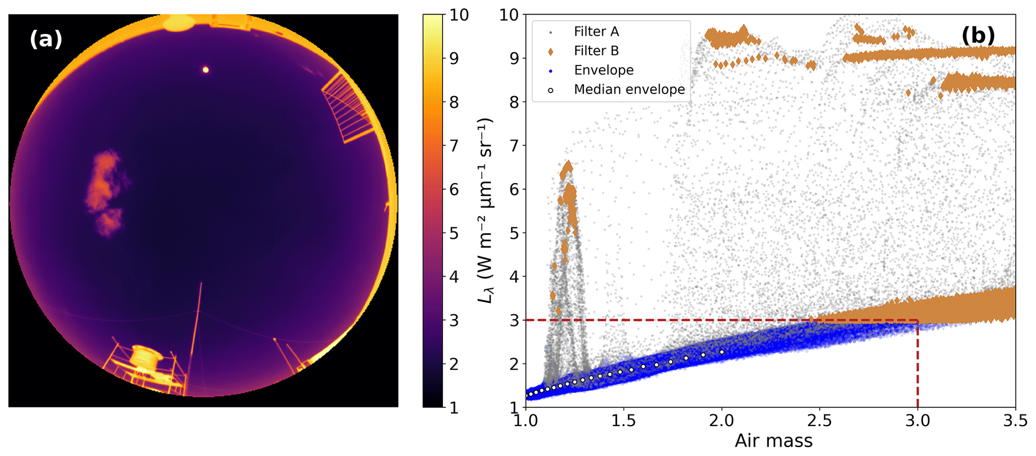
Figure 1 Spectral radiance (L_λ) measured at ASIVA’s channel 4 (i.e., 10–12 µm) on 6 July 2017 at 15:17 UTC (12:17 LT) in São Paulo: (a) calibrated radiance image; (b) L_λ plotted as a function of the air mass. Cloudy and physical structure pixels were eliminated by applying the procedure described in the text (Filters A and B). Envelope data points correspond to clear-sky L_λ, from which medians were computed at specific air mass values.

Downward spectral radiance can be determined for each image pixel, which is related to a specific angle of incidence of radiation. The zenithal and azimuthal view angles for each pixel are calibrated from the camera lens equation and the position of the sun over an entire day or, ideally, a summer day and a winter day. The gain of the camera for each pixel is radiometrically calibrated using a heated target blackbody, kept at a controlled temperature, by measuring the pixel count difference relative to a reference blackbody at room temperature, assuming a linear response of the sensor. More details on the instrument hardware and calibration are given elsewhere (Klebe et al., 2014). The pixel-level gain factor G_λ is calculated as

$$\begin{array}{}\text{(2)}& G_{\mathit{\lambda }}={\displaystyle \frac{C_{\mathit{\lambda }}\left(\mathrm{tar}\right)-C_{\mathit{\lambda }}\left(\mathrm{ref}\right)}{{\mathit{ϵ}}_{\mathit{\lambda }}\left({\mathrm{BB}}_{\mathit{\lambda }}\left(T_{\mathrm{tar}}\right)-{\mathrm{BB}}_{\mathit{\lambda }}\left(T_{\mathrm{ref}}\right)\right)}},\end{array}$$

where C_λ(tar) and C_λ(ref) are the measured count levels at the specified channel of central wavelength λ for the target and reference blackbodies, respectively; ϵ_λ is the emissivity of the bodies at λ; and BB_λ(T_tar) and BB_λ(T_ref) are the theoretical spectral radiances of a blackbody at the temperatures T_tar and T_ref, respectively (in units of $\mathrm{W}{\mathrm{m}}^{-\mathrm{2}}\mathrm{\mu }{\mathrm{m}}^{-\mathrm{1}}{\mathrm{sr}}^{-\mathrm{1}}$). This quantity is given by the integral of the Planck spectral radiative emission function over the detection spectral region, normalized by the system response:

$$\begin{array}{}\text{(3)}& {\mathrm{BB}}_{\mathit{\lambda }}\left(T\right)={\displaystyle \frac{\int \frac{\mathrm{1.19}\times {\mathrm{10}}^{\mathrm{8}}{\mathit{\lambda }}^{-\mathrm{5}}}{e^{\mathrm{1.44}\times {\mathrm{10}}^{\mathrm{4}}/\mathit{\lambda }T}-\mathrm{1}}{t}_{\mathit{\lambda }}\mathrm{d}\mathit{\lambda }}{\int t_{\mathit{\lambda }}\mathrm{d}\mathit{\lambda }}},\end{array}$$

where the wavelength λ is given in units of micrometer (µm) and t_λ is the effective system response, including the effects of filter and lens transmittance, as well as detector sensitivity (Klebe et al., 2014).

Sky spectral radiance measurements are obtained using an image of the sky and an image of the reference blackbody at a known temperature T_ref, positioned in a mobile hatch that slides open for an unobstructed view of the sky and closes for the reference measurement (see Fig. 1 in Klebe et al., 2014). The spectral radiance L_λ is then calculated for each pixel as

$$\begin{array}{}\text{(4)}& L_{\mathit{\lambda }}={\displaystyle \frac{C_{\mathit{\lambda }}\left(\mathrm{sky}\right)-C_{\mathit{\lambda }}\left(\mathrm{ref}\right)}{G_{\mathit{\lambda }}}}+{\mathrm{BB}}_{\mathit{\lambda }}\left(T_{\mathrm{ref}}\right),\end{array}$$

where C_λ(sky) and C_λ(ref) are the measured counts for the sky and reference images, respectively, and BB_λ(T_ref) is the theoretical spectral radiance of the blackbody at T_ref (Klebe et al., 2014). In theory, the first term in Eq. (4) $\left(C_{\mathit{\lambda }}\right(\mathrm{sky})/G_{\mathit{\lambda }})$ represents the spectral radiance of the sky. However, the experimental measurements are also influenced by infrared radiation emitted by nearby instrument components and even by the lens. In order to eliminate any unwanted local contribution, the measured spectral radiance of the blackbody $\left(C_{\mathit{\lambda }}\right(\mathrm{ref})/G_{\mathit{\lambda }})$ is subtracted from the signal, and its theoretical value BB_λ(T_ref) is added in such a way that any spurious contamination present in both sky and reference measurements are removed in the final result.

The spectral radiance can then be analyzed as a function of the observation geometry. In this work, we study the spectral radiance as a function of air mass, defined as $\mathrm{1}/\cos \left(\mathit{\theta }\right)$, where θ is the view zenith angle for each pixel. Figure 1 shows, as an example, L_λ measurements using ASIVA’s infrared channel 4. Figure 1a presents L_λ for each image pixel, and Fig. 1b shows L_λ as a function of air mass. The lower L_λ envelope in Fig. 1b, clearly defined, corresponds to the emission of cooler regions observed in the image, which are those of clear sky, while the points with greater radiance are warmer bodies such as clouds and nearby structures in the camera's view. It is expected that near the zenith the measured radiance for clear skies will be lower than in regions closer to the horizon. This is clearly observable in Fig. 1a and in the shape of the lower envelope in Fig. 1b. This is due to the thinner atmosphere between the camera and outer space at the zenith, with this thickness increasing with the air mass. Cloudy and partially cloudy pixels were identified and removed from the analyses by excluding pixels with either (a) high spatial L_λ variability or (b) values above a maximum L_λ threshold. The spatial variability filter was applied by computing, for a given pixel, the L_λ sample standard deviation for the eight nearest-neighbor pixels and removing cases with standard deviation above 0.07 $\mathrm{W}{\mathrm{m}}^{-\mathrm{2}}\mathrm{\mu }{\mathrm{m}}^{-\mathrm{1}}{\mathrm{sr}}^{-\mathrm{1}}$ (“Filter A” data points in Fig. 1b). The maximum L_λ threshold filter depends on the pixel air mass, the instrument temperature, and the cloud type possibly present (e.g., it can be more complex to exclude very cold thin cirrus clouds). This limit is defined, for a given temperature condition, as the median L_λ computed at air mass 3.00 ± 0.01. In the particular example shown in Fig. 1b, this threshold was 3.0 $\mathrm{W}{\mathrm{m}}^{-\mathrm{2}}\mathrm{\mu }{\mathrm{m}}^{-\mathrm{1}}{\mathrm{sr}}^{-\mathrm{1}}$, as indicated by the horizontal dashed line. Data points identified as “Filter B” in Fig. 1b were eliminated by the threshold filter. Finally, after applying filters A and B, the minimum L_λ envelope is defined as the median of L_λ, calculated for each ± 0.001 air mass interval, around discrete air mass values in the LUTs described further ahead for air masses below 2.0. These correspond to “Median envelope” data points in Fig. 1b. At the channel-4 range, the sky radiance L_λ strongly depends on the amount of columnar PWV, its vertical distribution and temperature, the optical path from the emission to the sensor, and the transmittance of the medium. Using radiative transfer simulation software, such as libRadtran, the expected L_λ as a function of air mass can be calculated for a series of atmospheric humidity profiles. A PWV retrieval can be obtained by determining, for a given humidity profile, which of the simulations most closely matches the measured lower envelope such as the one shown in Fig. 1b.

The ASIVA sky imager was installed at the Institute of Physics, University of São Paulo (23.56^∘ S, 46.74^∘ W; 786 m a.s.l.), and operated during three different periods: from 5–22 July 2017 (the 2017 austral winter) with high acquisition frequency (images every 3 min, approximately); from 1–23 February 2018 (the 2018 summer), producing images every 20 min; and from 20 July–24 August 2018 (the 2018 winter), imaging the sky every 30 min.

2.2 Sun photometer PWV retrievals

An AERONET sun photometer (Holben et al., 1998), colocated with the ASIVA sky imager (23.56^∘ S, 46.74^∘ W; 786 m a.s.l.), was used to independently assess columnar PWV retrievals. The sun photometer is equipped with a collimated photodetector that measures solar and sky radiance at different wavelengths. The integrated PWV content is determined from the attenuation of solar radiation at 940 nm along its optical path in the atmosphere by applying a modified Beer–Lambert–Bouguer law (Pérez-Ramírez et al., 2014). Only level-2.0 calibrated PWV data from AERONET (Smirnov et al., 2000) were used in this work. According to Pérez-Ramírez et al. (2014), sun photometer results can have systematic calibration uncertainties corresponding to 4 %–5 % of the PWV retrievals and random radiance measurement uncertainties below 1 %. Besides that, simplifications in modeling the atmospheric water vapor radiative transmission process can lead to about a 5 % PWV uncertainty. Hence, the final number of 10 % uncertainty in AERONET PWV retrievals that has been quoted in the literature corresponds to a composition of all these sources of errors, which is the figure used in this work.

AERONET PWV retrievals have been performed in São Paulo from November 2000 to the present day, with some gaps from February 2012 to November 2014 (Hack, 2023a). We used the AERONET retrievals in two different ways in this work. First, all available PWV retrievals were used in comparison with radiosonde data. This was done by averaging sun photometer retrievals within ± 30 min of each 12:00 UTC (09:00 LT) sounding launch. Secondly, AERONET and ASIVA PWV retrievals were compared on selected days with clear skies or few clouds.

2.3 Vertical water vapor profiles and integrated PWV

Radiosondes have been regularly launched from the Campo de Marte Airport (International Civil Aviation Organization code SBMT; latitude, longitude: 23.52^∘ S, 46.63^∘ W; altitude: 722 m a.s.l.) at 00:00 and 12:00 UTC (21:00 and 09:00 LT, respectively). The airfield is 11 km distant, and 64 m below in altitude, from the ASIVA and sun photometer operation site. Direct measurements of the specific humidity along the vertical radiosonde profile are integrated to yield the PWV for each radiosonde launch. Castro-Almazán et al. (2016) argue that calibration biases can lead to up to 5 % uncertainty in the retrieved PWV by radiosondes. They also indicate that daytime radiosonde launches can have a dry bias of 2 %–8 % due to the solar heating of the humidity sensor. Following the results from a semiempirical analysis by Castro-Almazán et al. (2016), we use in this work a figure of 3 % uncertainty for radiosonde PWV retrievals. All radiosonde data were accessed via the University of Wyoming website (https://weather.uwyo.edu/upperair/sounding.html, last access: 19 August 2022 12:00 UTC).

Radiosonde data (Hack, 2023a) were used in this work in multiple ways that will be discussed in greater detail further ahead. Firstly, when available, a radiosonde vertical profile at 09:00 LT is used to derive one type of LUT where L_λ is simulated for a range of PWV values. This is done by normalizing the given radiosonde profile to match each PWV in the simulated range. In this way, the computed LUT represents what downwelling radiance would be expected if the relative vertical distribution of humidity were given by the radiosonde profile for a range of different PWV values. Secondly, a total of 10 years (2005 to 2015) of summertime and wintertime radiosonde data were aggregated to derive seasonal average atmospheric profiles. These São Paulo seasonal profiles were used in comparison to other literature profiles (e.g., “tropical profile”; Anderson et al., 1986) to assess how each of them fares when used to compute L_λ with respect to the measured L_λ. Thirdly, wintertime radiosonde profiles were used to build simplified synthetic profiles that will be addressed in the next section. These synthetic profiles capture the range of vertical variability in the median distribution of humidity. Finally, all 09:00 LT PWV radiosonde data available from 2000–2019 were used in comparison with AERONET retrievals, as discussed previously.

2.4 Synthetic moisture profiles

Besides PWV, one critical issue in computing the theoretical L_λ expected at the surface level is the water vapor vertical distribution. The intensity of downwelling radiation is inversely proportional to the square of the distance between the emitting parcel and the detector. Furthermore, the signal will be attenuated more by interaction with the atmosphere, depending on the length of the optical path. It is also important to note that the closer the bulk of water vapor molecules is to the surface, the higher its temperature and the greater its radiative emission; hence, the higher the measured L_λ on the ground will be.

If radiosonde data are not available to clearly define the humidity profile in a given day, one has to resort to hypothetical vertical distributions, such as the tropical profile from libRadtran (Emde et al., 2016), or seasonal average profiles for the specific location. In addition to examining these solutions in the Results section, we also built simplified synthetic moisture profiles, based on the observed wintertime variability of the vertical distributions of water vapor for the study site. The key issue these synthetic profiles seek to solve is only the “relative” vertical distribution of water vapor. That is to say, how far from the surface the median distribution of water vapor is, regardless of the absolute PWV value. The reason for this is that in LUT calculations such relative water vapor distributions are used, and the integral PWV is normalized to a specific value.

The variability of the vertical profile of water vapor was studied on winter days with clear skies or few clouds. Winter was used as it is the season with the majority of available measurements since it is drier in São Paulo (i.e., lowest yearly PWV observed) and therefore with less frequent clouds than summer. A dataset with radiosondes at 09:00 LT for the austral winter months (July–September) was scrutinized to select profiles that represented conditions with less cloud cover. This was done by taking the frequency of AERONET PWV retrievals within ±30 min from the radiosonde launching time as a proxy for the occurrence of clouds. Radiosonde profiles were retained for analysis whenever at least five sun photometer retrievals were successful within the 1 h matching window. The median humidity altitude in the radiosonde subset was investigated to identify typical “low-altitude” and “high-altitude” profiles, regardless of their absolute PWV, and average profiles were computed (Fig. 2). From these, synthetic simplified versions of such profiles were built by visual inspection. A profile corresponding to “medium altitude” was computed as the average between the low- and high-altitude profiles. Figure 2 shows the three resulting synthetic profiles, which are meant to be used when no radiosonde information is available for a given day, as described further below. Table 1 shows the data points used in the profiles. The same synthetic profiles were used for summer PWV retrievals, i.e., by keeping the same relative vertical distribution of water vapor, while the method retrieves PWV values within the expected range for summer. Even though there will always be discrepancies between real radiosondes and synthetic profiles, in general such differences show little influence on the final integrated PWV.

Table 1 Synthetic atmospheric humidity profiles shown in Fig. 2.

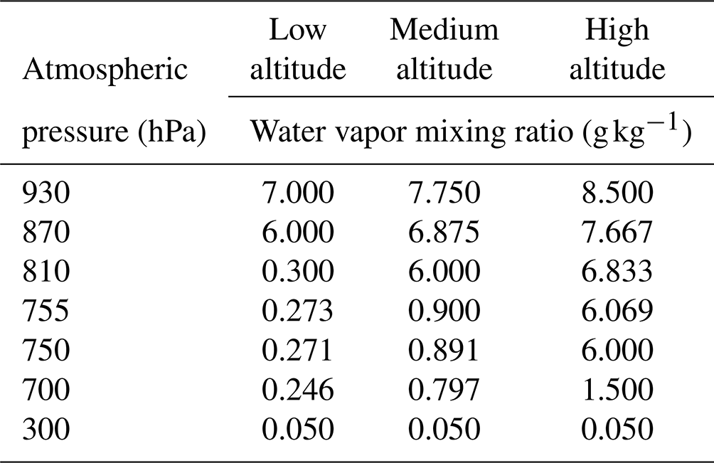
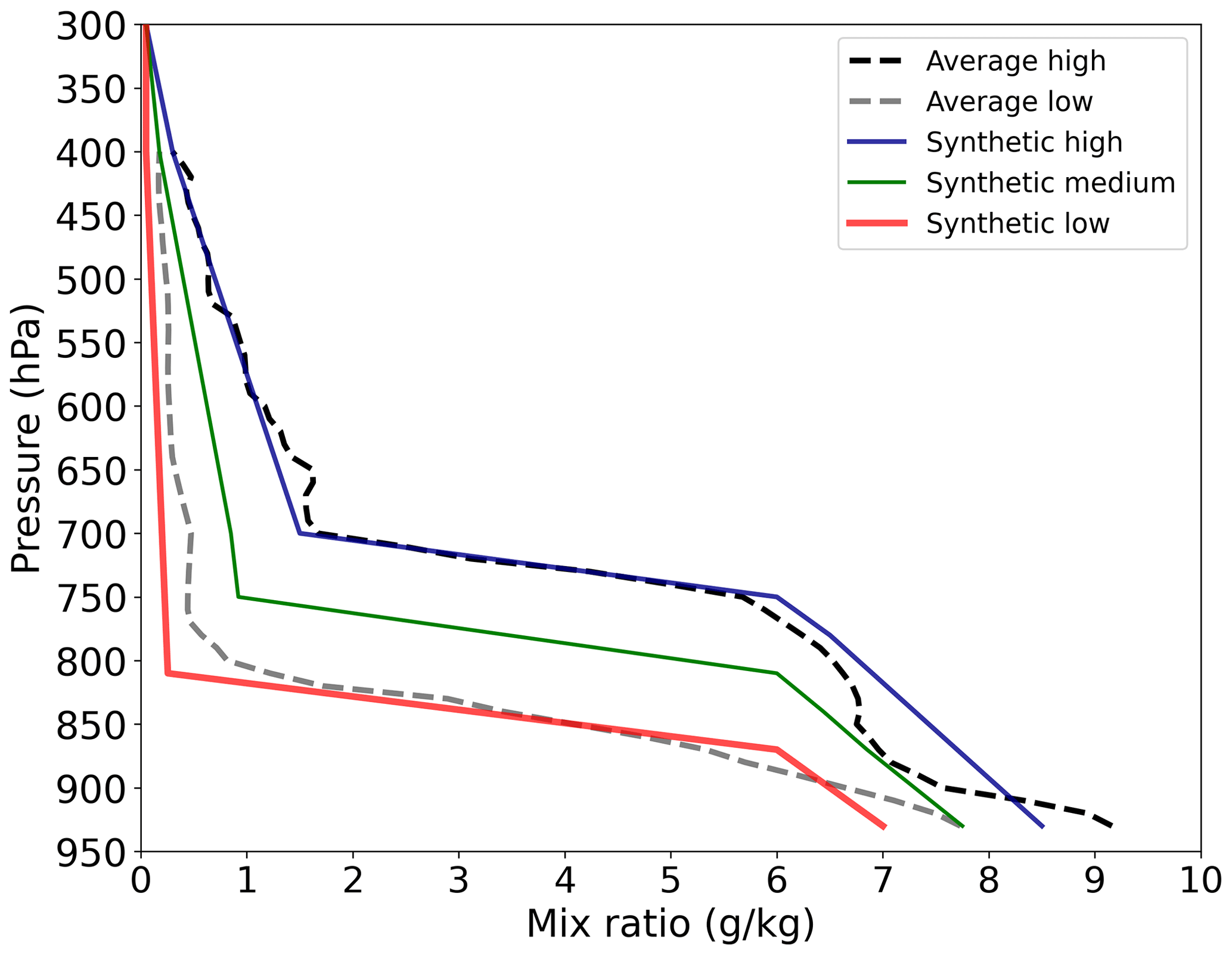
Figure 2 Simplified synthetic humidity profiles that describe the observed variability of winter radiosonde profiles. The high-altitude (blue) and low-altitude (red) synthetic profiles were based on average profiles of radiosonde data from 2016–2019, shown as black and gray dashed curves. The medium-altitude synthetic profile (green) is an intermediate between the high- and low-altitude profiles.

Figure 3 Method flow diagrams depending on the availability of radiosonde data: (a) ASIVA PWV retrievals without radiosonde data and (b) with additional radiosonde information at 09:00 LT (12:00 UTC).

2.5 Radiative transfer simulations

In this work, we used the libRadtran software package, which is a library for atmospheric radiative transfer calculations (Emde et al., 2016; Mayer and Kylling, 2005). The program solves the radiative transfer equation for a given atmospheric setup and then obtains simulated radiances and irradiances for a specified viewing geometry. We used the DISORT (DIScrete Ordinate Radiative Transfer) method to solve the radiative transfer equation and the plane-parallel atmosphere approximation. Internal and user-provided atmospheric humidity profiles were used in different steps of the work. Three internal standard atmospheric profiles were studied: tropical, midlatitude summer, and midlatitude winter (Anderson et al., 1986), seeking to understand how they might represent the physical conditions at the observing site. Even though the site location is in the subtropics, midlatitude profiles were included in the analyses for the sake of comparison. We also used average seasonal atmospheric profiles as input, obtained from radiosonde data from 2005 to 2015, to study the influence of the vertical distribution of humidity on simulated L_λ.

Figure 4 (a) Sampling site location in São Paulo, Brazil (23.56^∘ S, 46.74^∘ W; 786 m a.s.l.). (b) Comparison between level-2.0 AERONET sun photometer (SP) PWV retrievals and radiosonde (RS) integrated PWV from 2001 to 2019. The regression result is shown as a continuous red line. The 1:1 line is shown dashed. SP data were temporally matched within 30 min to daytime RS launches at 09:00 LT (12:00 UTC). The RS launch site is located 11 km from and at an altitude 64 m below the sampling site. To avoid cloudy cases, only days with at least five SP retrievals within the temporal window were considered. MB and RMSD are the mean bias and the root-mean-square deviation of RS with respect to SP data.

Two types of LUTs were computed with libRadtran in this study. Firstly, when radiosonde data are not available, a LUT of simulated $L_{\mathit{\lambda },i}^{\mathrm{c},\mathrm{s}}$ as a function of air mass was produced for the high-, medium-, and low-altitude synthetic humidity profiles (presented in Sect. 2.4). The “c” and “s” superscripts indicate calculated radiances for the synthetic profiles. The “i” subscript indicates the three possible profiles (i=1, 2, 3). The LUT integrated PWV varied from 5.0 to 40.0 mm in increments of 0.1 mm. By using this PWV range, the LUT covers the scope of all available winter and summer measurements at the sampling site. Air masses were simulated for 21 values from 1.0 to 2.0, corresponding to a maximum view zenith angle of 60^∘. Another LUT of simulated $L_{\mathit{\lambda }}^{\mathrm{c},\mathrm{p}}$ is computed when a humidity profile is available from a 09:00 LT radiosonde launch. The “p” superscript indicates that the LUT is to be computed using a radiosonde profile. In this case, the simulation uses the same configurations described above, except that the relative vertical humidity distribution is taken from the radiosonde profile. The rationale here is to assume that the profile information taken at 09:00 LT remains constant throughout the day, thus allowing for deriving PWV retrievals using this LUT.

2.6 Method description

The ASIVA PWV retrieval method depends on the availability of radiosonde data that inform the vertical distribution of humidity at the sampling site. Figure 3 shows a diagram depicting two basic pathways to retrieve PWV, for cases where no radiosonde data are available for a specific day, and a different path when such data can be employed. Ultimately, the precision of PWV retrievals is linked to the degree at which the vertical distribution of water vapor is known.

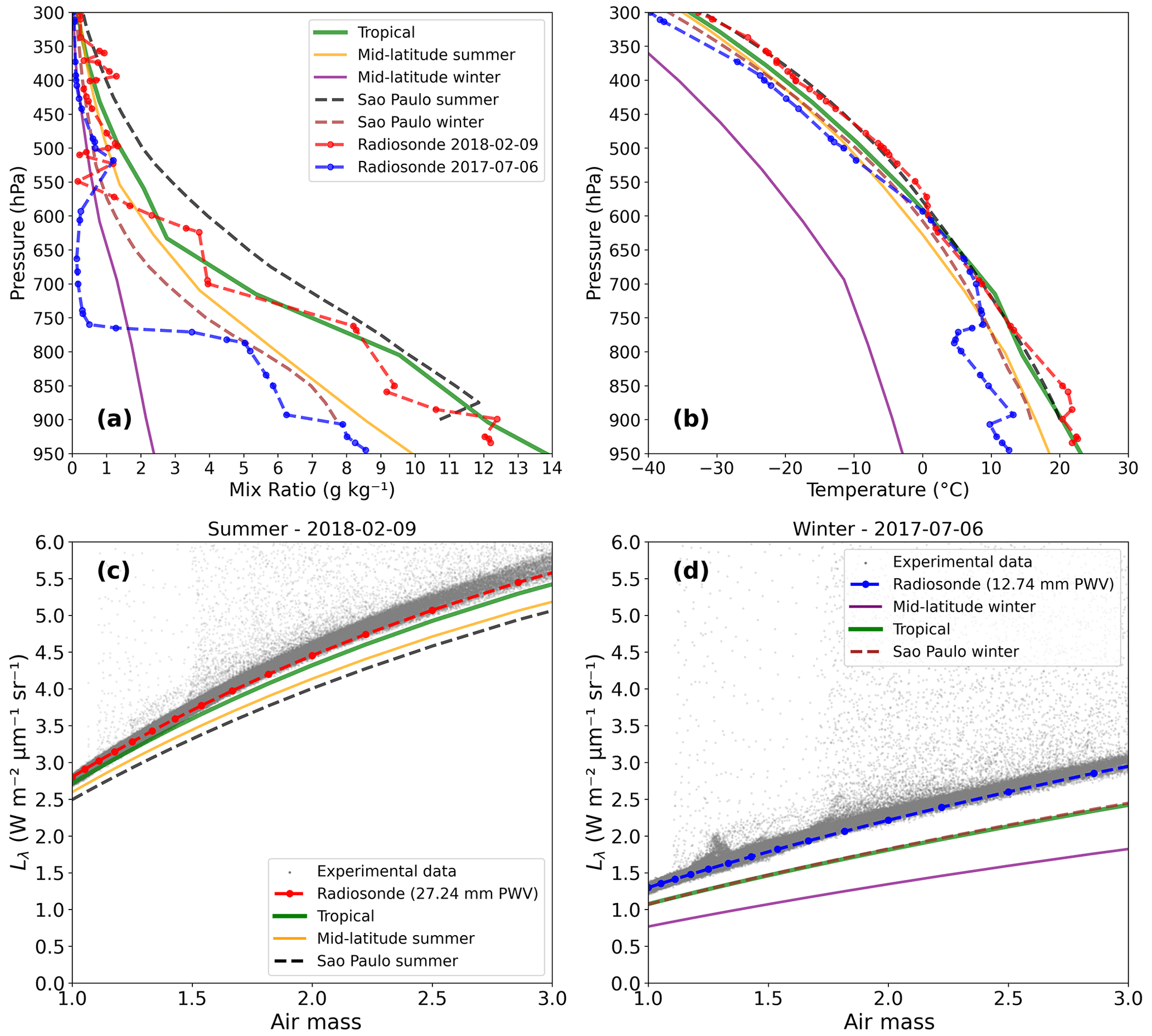
Figure 5 (a) Water vapor mixing ratio and (b) temperature vertical profiles for tropical (green), midlatitude summer (orange), and midlatitude winter (purple) standard atmospheric models, as well as climatological averages for São Paulo in summer (black) and winter (brown), with examples for a summer day (9 February 2018, red) and a winter day (6 July 2017, blue). Measured L_λ (gray) for (c) 9 February 2018 and (d) 6 July 2017, compared to libRadtran simulations for each atmospheric profile model. Radiance measurements were made within a few minutes from each 09:00 LT radiosonde launch. Notice that São Paulo winter and tropical profile curves are nearly coincident in panel (d). The simulations used the relative vertical moisture distribution in each profile, normalizing them to the PWV measured by the radiosonde.

When no radiosonde data are available (Fig. 3a), the method relies on the three-profile $L_{\mathit{\lambda },i}^{\mathrm{c},\mathrm{s}}$ LUT discussed above, derived from previous knowledge about the typical distribution of water vapor over the sampling site. The measured $L_{\mathit{\lambda }}^{\mathrm{m}}$ values were processed to remove cloudy pixels and by selecting only the lower envelope of the $L_{\mathit{\lambda }}^{\mathrm{m}}$ vs. air mass data. The measured envelope radiance medians, in air mass intervals of ± 0.001 around the simulated air masses, were compared to the 21 simulated $L_{\mathit{\lambda },i}^{\mathrm{c},\mathrm{s}}$ values in the LUT to find the amount of PWV that minimizes the sum of squared differences δ²= ($L_{\mathit{\lambda }}^{\mathrm{m}}$-$L_{\mathit{\lambda },i}^{\mathrm{c},\mathrm{s}}{)}^{\mathrm{2}}$ for each of the i=1, 2, 3 profiles. At this point, we get three time series, noted as PWV_i, with each one corresponding to a different median altitude for the vertical distribution of water vapor (circled “1” in Fig. 3a). To choose from the three options, one can use statistics on atmospheric profiles for the specific location and time of the year or else choose the medium-altitude profile if no additional information is known. In the case when there are partial AERONET PWV data, e.g., on a cloudy day when few AERONET retrievals are successful, a comparison between the AERONET PWV to the PWV_i retrieval time series can be used to discriminate between the three options. In this situation, we derive a single “best” PWV time series; hence, we additionally get information about the median vertical distribution of water vapor, since we are able to distinguish between the three altitude profiles (indicated “2” in Fig. 3a). Finally, in the case when a full AERONET PWV time series is available, a comparison with the retrieved ASIVA PWV_i can be used to analyze qualitatively altitude variations in the median distribution of water vapor. Since the method originally results in three PWV time series, corresponding to each of the altitude profiles, the relative closeness between AERONET PWV and each ASIVA PWV_i time series can be a proxy for the median water vapor altitude or its change over time (“3” in Fig. 3a).

If a 09:00 LT radiosonde profile is available, the retrieval method follows the flow diagram in Fig. 3b. It is assumed that the relative vertical humidity distribution remains constant throughout the day. With the specific profile and the array filter function as inputs, a LUT is organized from the calculated $L_{\mathit{\lambda }}^{\mathrm{c},\mathrm{p}}$, considering the PWV and air mass ranges described above. Next, two options for the PWV retrieval are possible. First, taking a time series of the measured $L_{\mathit{\lambda }}^{\mathrm{m}}$ envelope as a function of air mass, we minimize the difference δ²= ($L_{\mathit{\lambda }}^{\mathrm{m}}$-$L_{\mathit{\lambda }}^{\mathrm{c},\mathrm{p}}{)}^{\mathrm{2}}$ between measurements and LUT entries to yield a time series of the average columnar PWV over the sampling site for that specific day (marked as a circled “4” in Fig. 3b). Another possibility is the pixel-level retrieval of PWV from a single $L_{\mathit{\lambda }}^{\mathrm{m}}$ sky mapping. In that case, a linear interpolation is applied to the $L_{\mathit{\lambda }}^{\mathrm{c},\mathrm{p}}$ LUT, such that a function is derived to relate the calculated PWV and $L_{\mathit{\lambda }}^{\mathrm{c},\mathrm{p}}$ for each pixel air mass in the acquired imagery. The final step is to apply another linear interpolation, project the actual $L_{\mathit{\lambda }}^{\mathrm{m}}$ measurement onto the derived function, and achieve the pixel-level PWV retrievals. The resulting PWV sky mapping (“5” in Fig. 3b) can reveal azimuthal water vapor inhomogeneities (“6” in Fig. 3b) that can be used, for instance, for analyses of horizontal vapor transport. Examples of all retrievals described in Fig. 3 are shown in the Results section. The software code suite used in this study is available elsewhere (Hack, 2023b).

3 Results

3.1 AERONET and radiosonde PWV retrievals

In São Paulo, PWV retrievals are available from regular radiosonde profiles and from an AERONET sun photometer administered by the National Aeronautics and Space Administration (NASA) (Holben et al., 1998). Figure 4 shows a comparison between both instruments at the sampling site, between 2001 and 2019. In order to minimize the influence of clouds, we only considered matching data points when at least five AERONET PWV retrievals were successful within a 1 h time window centered on the 09:00 LT radiosonde launch time. PWV uncertainty was assumed to be 10 % for sun photometer retrievals (Pérez-Ramírez et al., 2014) and 3 % for radiosondes (Castro-Almazán et al., 2016).

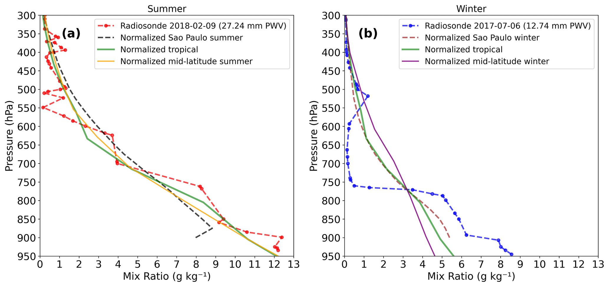
Figure 6 Vertical water vapor mixing ratio profiles normalized to the radiosonde integral PWV values for (a) a summer day (9 February 2018) and (b) a winter day (6 July 2017). Atmospheric profile coloring is the same as in Fig. 5.

Figure 4 shows that the PWV varies from around 5.0 mm on the driest days (usually in austral winter) to almost 40.0 mm on the most humid days (summer). The radiosonde PWV shows a positive mean bias (MB) of 0.75 mm relative to AERONET retrievals and a root-mean-square deviation (RMSD) of 1.9 mm. The observed bias may be in part due to the different locations where the two measurements were performed (11 km horizontal distance, 64 m altitude difference). A linear regression of radiosonde PWV against AERONET retrievals resulted in an angular coefficient of 1.039 ± 0.016 and a linear coefficient of −0.15 ± 0.19 mm, with R²=0.93. This indicates that both instruments are in general agreement, with radiosonde results slightly above sun photometer retrievals, on average. However, the dispersion of data points is considerably larger for summer (i.e., larger PWV), indicating a poorer correspondence during that season. On some summer days, the radiosonde can show a PWV of more than 10.0 mm higher than the AERONET retrieval. Taking a subset of the data for which the AERONET PWV is above 20.0 mm, the resulting MB was 1.5 mm, and the RMSD was 3.0 mm.

3.2 Vertical profiles of water vapor and L_λ measurements

Figure 5 presents the mixing ratio and temperature profiles (Fig. 5a and b, respectively) for the standard tropical, midlatitude summer, and midlatitude winter atmospheric profiles (Anderson et al., 1986), as well as seasonal (summer and winter) radiosonde averages for São Paulo. Figure 5a and b also show radiosonde data for specific days of austral summer (9 February 2018) and winter (6 July 2017). São Paulo is located at the threshold between the tropics and subtropics. The midlatitude profiles are only included in Fig. 5 for the sake of comparison. These vertical profiles were used as input to libRadtran L_λ simulations with the PWV integral column normalized to the value measured by the radiosonde. The results are shown in Fig. 5c and d for summer and winter, respectively, and compared to the ASIVA experimental data.

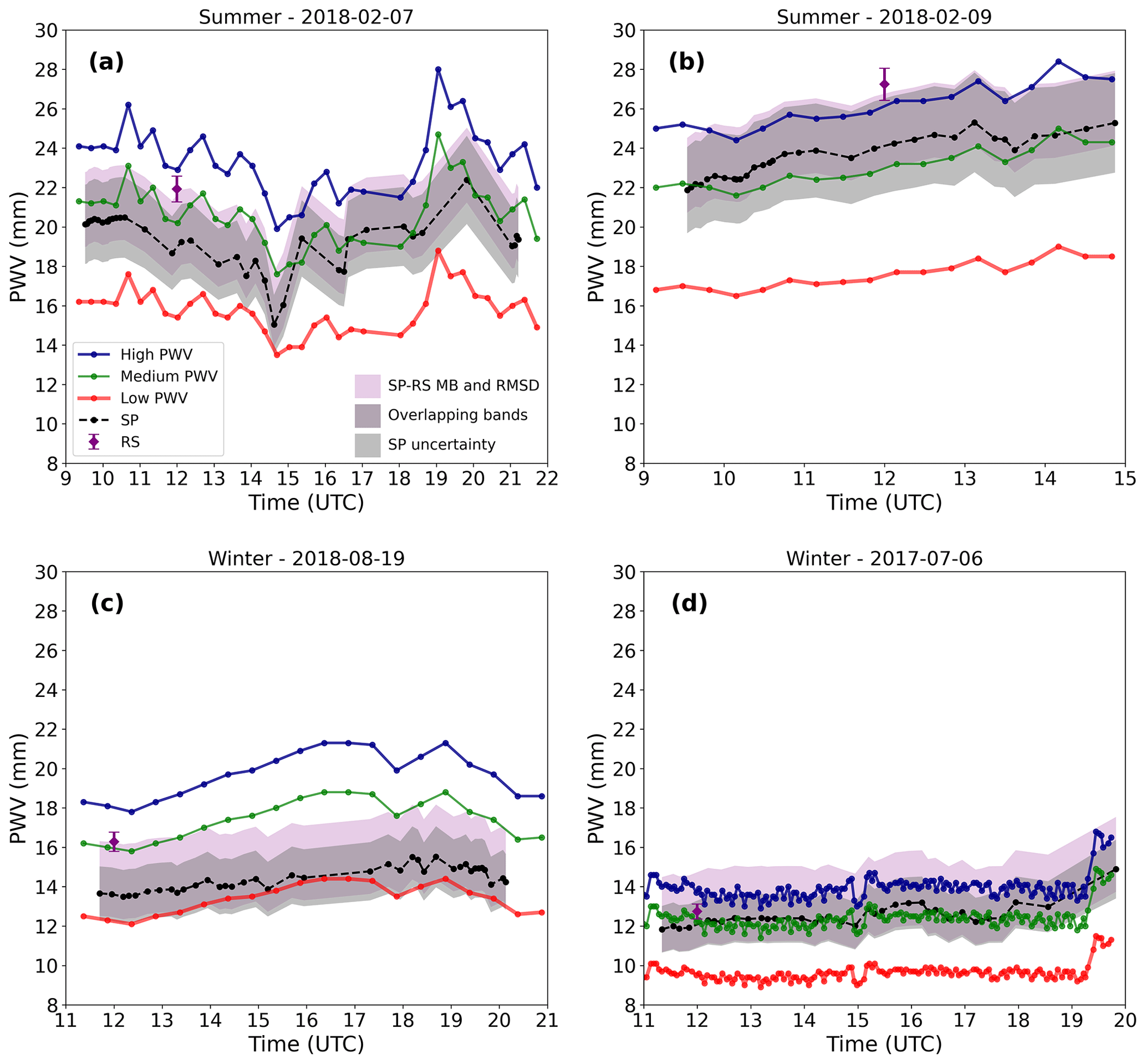
Figure 7 Examples of ASIVA PWV retrieval time series using synthetic profiles compared to AERONET sun photometer (SP, black) and radiosonde (RS, purple) for two summer days, (a) 7 February 2018 and (b) 9 February 2018, and two winter days, (c) 19 August 2018 and (d) 6 July 2017. The retrievals use the high-altitude (blue), medium-altitude (green), and low-altitude (red) simplified synthetic vertical profiles presented in Fig. 3 under the method described in Sect. 2.6. The darker gray shading indicates the nominal SP retrieval uncertainty of 10 %. The RS error bar corresponds to a 3 % uncertainty. The purple shading indicates the observed MB and RMSD when comparing SP and RS retrievals from Fig. 4.

A comparison between Fig. 5a and b indicates that, for this case, the vertical profile of water vapor shows a much greater percentage variation than the temperature profile. The variations in temperature are small with the exception of the midlatitude winter model, which proves to be very different from the radiosondes. None of the standard atmospheric profiles fits the real conditions of São Paulo's atmosphere, although the tropical model seems to be a better option, with the vertical water vapor distribution closest to the surface. The midlatitude summer profile is the closest to the average of radiosondes for winter (marked as “Sao Paulo winter” in Fig. 5).

Comparing Fig. 5c (summer) and 5d (winter), when PWV was 27.24 and 12.74 mm, respectively, the measured and simulated L_λ values for the summer day are almost twice as high as on the winter day. In both cases, only the libRadtran simulations using the specific radiosonde profile for each day match the measured L_λ envelope; all other simulations show biases toward smaller values. These L_λ observed biases are higher in the winter (Fig. 5d) than in the summer (Fig. 5c).

The simulations using the standard tropical profile and the São Paulo winter profile (Fig. 5d) show very similar L_λ values due to the nearly coincident shape of their relative vertical humidity distribution. To highlight differences in the relative vertical humidity distribution, artificial profiles were computed by normalizing each of them to the same integral PWV value. Fig. 6 shows the vertical profiles used in Fig. 5 after the normalization procedure. In Fig. 6a, the normalized tropical profile shows that its vertical humidity distribution is closer to the surface when compared to the normalized midlatitude summer or the normalized São Paulo summer profiles. These differences in the vertical humidity distribution are even more pronounced in the winter profiles in Fig. 6b, where we see the contrasting features for each of the profiles. At pressure levels below about 800 hPa, the normalized tropical and average São Paulo winter profiles are similar; however, both are very different from the example radiosonde for 6 July 2017. The conclusion is that besides the integral PWV value, the relative vertical distribution of humidity is also a key factor in modeling the observed L_λ, as shown in Fig. 5d, and the radiosonde profile for the specific day under analysis is the best option to describe the humidity distribution.

3.3 Retrieved PWV time series

Following the method described in Sect. 2.6, we start by showing results for PWV retrievals when no radiosonde data are available on a specific day. Measured L_λ vs. air mass envelopes were compared to simulated L_λ for the high-, medium-, and low-altitude synthetic humidity profiles to retrieve the PWV. Figure 7 shows the resulting ASIVA PWV time series for two summer days (Fig. 7a and b) and two winter days (Fig. 7c and d). The radiosonde PWV and the AERONET sun photometer time series are shown in Fig. 7 for context. The ASIVA PWV retrievals are highly sensitive to the assumed vertical distribution of humidity represented by the synthetic profiles, as expected from Fig. 5. The three PWV time series indicated in Fig. 7 examples as red, green, and blue datasets correspond to the circled “1” solution in the method flow diagram (Fig. 3a). In case no other piece of information is available, one can consider the PWV time series represented by the typical seasonal average vertical distribution of water vapor, defined by the medium-altitude (green) profile, which in general approximates better AERONET PWV retrievals. However, notice in Fig. 7c that occasionally the medium-altitude profile will be biased with respect to AERONET, since the natural variability of the humidity profiles for this location is shown by the range between low- and high-altitude synthetic profiles (red and blue curves).

On partially cloudy days, it is possible to have some AERONET PWV retrievals when the sun is unobstructed by clouds. For instance, Fig. 7a shows many AERONET retrievals at the beginning of the day (∼10:00–11:00 UTC) and fewer in the afternoon when it is cloudier (∼19:00–20:00 UTC). By comparing a few AERONET PWV retrievals on such occasions with the three ASIVA PWV time series, one can gauge which profile is most appropriate to represent the atmospheric humidity distribution state. This “best solution” approach would result in the medium-altitude PWV time series being selected in Fig. 7a, b, and d and the low-altitude PWV time series in Fig. 7c. This outcome corresponds to the solution circled “2” in Fig. 3a.

On less cloudy days in which a longer AERONET dataset is available, it is possible to get more information than just the PWV by combining AERONET and ASIVA retrievals. Because the ASIVA synthetic three-profile method relies on a fixed altitude for each humidity distribution, one can infer the effective median altitude of the humidity distribution by comparing the time series from the two instruments. For instance, in Fig. 7b the AERONET PWV time series is consistently above ASIVA’s medium-altitude profile, and both series show a similar temporal trend and variability. If the ASIVA retrievals were to match AERONET, we would need to use a synthetic profile with a slightly more elevated median for the humidity distribution than the one in the medium-altitude profile (see Fig. 2). Thus, provided that both the temporal trend and variability from the two series can be considered equivalent, the PWV distance between them can be seen as a proxy for the effective median humidity distribution along the vertical direction. Notice in Fig. 7b that both the medium- and high-altitude ASIVA profiles (green and blue curves) are within the nominal AERONET uncertainty interval and the expected RMSD when comparing AERONET to radiosondes (Fig. 4).

Figure 7c shows an example of wintertime AERONET PWV retrievals close to but consistently above the ASIVA results in the low-altitude profile, with few AERONET retrievals between ∼15:00 and 17:00 UTC. This corresponds to a median humidity distribution altitude slightly above the one shown for the low-altitude profile in Fig. 2. In Fig. 7a, notice that AERONET retrievals are situated between ASIVA’s low- and medium-altitude time series from ∼09:00–15:00 UTC (∼06:00–12:00 LT), with a descending temporal trend in the PWV, and they then shift to roughly match ASIVA’s medium-altitude time series in the afternoon, with an increasing trend. This is consistent with an increased afternoon convective activity on that summer day, which typically involves moisture convergence over the site. The uncertainty bands around AERONET retrievals are mostly coherent with the medium-altitude ASIVA time series.

In contrast, the very stable and dry winter day shown in Fig. 7d shows AERONET and the medium-altitude ASIVA time series matching during most of the day. ASIVA was operated at a high frequency of acquisition of about one image every 3 min. After about 18:00 UTC, only three AERONET PWV retrievals were possible due to increased cloud cover. AERONET results show little variation in the retrieved PWV, with a range only slightly above 1.0 mm from about 11:00–19:00 UTC (08:00–16:00 LT). Due to the stable atmospheric conditions on that day, we take the AERONET results as a reference between 12:00 and 14:00 UTC to be compared to ASIVA results. The average of 35 ASIVA medium-altitude retrievals was 12.01 mm, which is about 2.8 % below the AERONET average PWV of 12.35 mm (10 retrievals). For this same time period, ASIVA’s precision was estimated as the sample standard deviation of 0.23 mm or approximately 1.9 % of the average ASIVA PWV. These considerations for a proxy to estimate an effective humidity median altitude correspond to the solution type circled “3” in Fig. 3a.

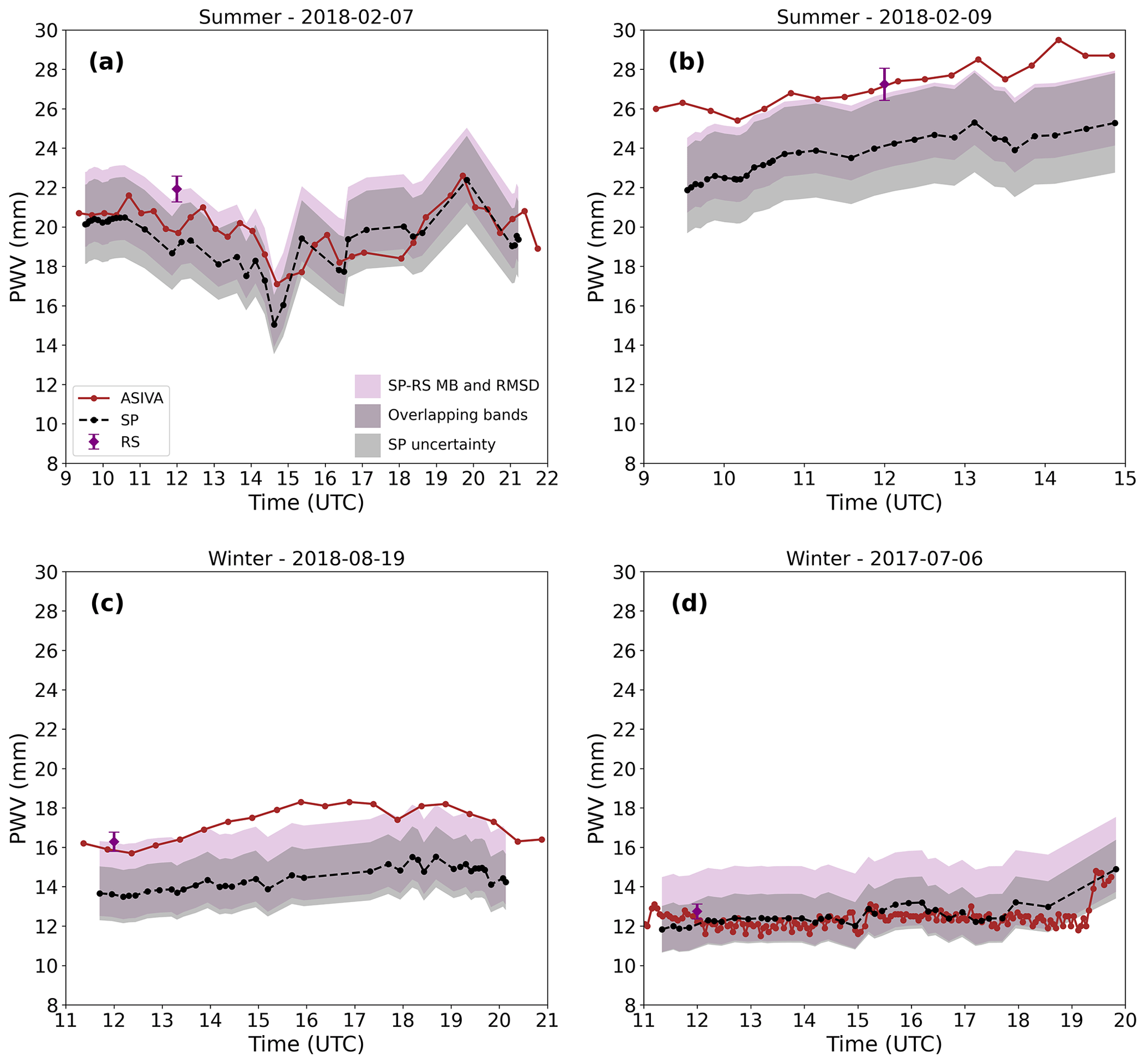
Figure 8 Examples of ASIVA PWV retrieval time series (brown) using specific 09:00 LT (12:00 UTC) radiosonde profiles for each case compared to AERONET (black) and radiosonde (purple) for two summer days, (a) 7 February 2018 and (b) 9 February 2018, and two winter days, (c) 19 August 2018 and (d) 6 July 2017. Shaded bands and radiosonde error bars are the same as in Fig. 7.

Now we turn the analysis to the particular case when a radiosonde profile is available for the specific day under consideration. In general, using a radiosonde profile will result in a better fit to the measured L_λ than resorting to average or synthetic profiles (see Fig. 5). However, the comparison between radiosonde and AERONET results can be significantly noisy for some days (Fig. 4). The measured $L_{\mathit{\lambda }}^{\mathrm{m}}$ vs. air mass envelopes were compared to the LUT with simulated $L_{\mathit{\lambda }}^{\mathrm{c},\mathrm{p}}$, calculated using the specific radiosonde data for the days we studied. Figure 8 shows the AERONET and ASIVA radiosonde PWV retrievals for the same cases shown in Fig. 7. For the summer and winter days in Fig. 8a and d, there is a close agreement between ASIVA and AERONET time series, including temporal trends in each day. Differences in the retrieved PWV are within about 2.0 mm in Fig. 8a and 1.0 mm in Fig. 8d, and they sit within the expected AERONET uncertainty range.

Figure 8b shows that the ASIVA PWV time series is consistently higher than AERONET but with similar temporal trends and variability. In particular, notice the radiosonde PWV is compatible with an interpolation of ASIVA retrievals around 12:00 UTC, within the 3 % radiosonde uncertainty, which is not always the case (e.g., Fig. 8a). Among the 4 measurement days presented in Fig. 8, this is the case with water vapor distributed higher in the atmosphere and also higher PWV. In the summer, like in this particular case, there is considerably more scattering when comparing radiosondes to AERONET retrievals, as discussed in Fig. 4. Therefore, a larger spread between these results is expected in this case and in the ASIVA time series, since it is derived from the radiosonde data. In this context, we consider the ASIVA retrievals in Fig. 8b to be adequate with respect to AERONET, regardless of the gap between the two time series.

Figure 8c apparently shows the larger discrepancy between ASIVA and AERONET time series in the Fig. 8 examples. There is coherence between the two series in the early morning (∼11:00–13:00 UTC) and in the afternoon (∼18:00–20:00 UTC) in the sense that both show temporal variations in the same direction. There are no AERONET data between ∼16:00–17:30 UTC. The core of the disparities occurs between about ∼13:00–16:00 UTC when the ASIVA series shows a higher positive slope in the increasing PWV compared to AERONET. This case in particular corresponds to an extreme winter condition in the radiosonde vs. AERONET comparison in Fig. 4; that is, the matching point sits at the very edge of the data cloud. The largest PWV discrepancy between the two series at ∼16:00 UTC is about the same size as the differences discussed in Fig. 8b. The ASIVA PWV around 12:00 UTC is compatible with the radiosonde data point within the 3 % uncertainty range. The retrieved ASIVA PWV time series in Fig. 8b is very similar to the solution using the medium-altitude synthetic profile (green curve in Fig. 7c). The conclusion here is that there are inherent discrepancies between the source radiosonde data and the AERONET PWV retrieval for this particular complex case. Hence, the radiosonde-derived ASIVA series will also show differences from the AERONET results. Such differences, however, are still under the variations that can be expected statistically. The ASIVA retrieval results discussed in Fig. 8, based on radiosonde profile data, correspond to the solution circled “4” in Fig. 3b.

Table 2 ASIVA, sun photometer, and radiosonde PWV retrieval statistics for the cases shown in Figs. 7 and 8.

^∗ SH F7, SM F7, and SL F7 refer to the ASIVA retrievals in Fig. 7 using the synthetic high-, medium-, and low-altitude profiles, respectively. RS F8 is the ASIVA retrieval using the radiosonde profile in Fig. 8.

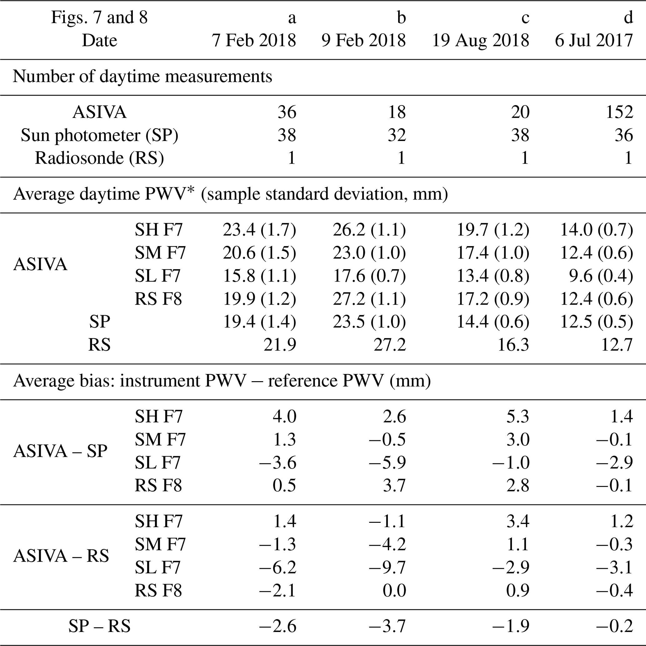
Table 2 shows a summary of PWV statistics for ASIVA, sun photometer, and radiosonde retrievals for the cases analyzed in Figs. 7 and 8. Although the PWV can vary during the day, Table 2 shows the daytime number of samples, average, and sample standard deviation for the three instruments, for the sake of comparison. The ASIVA instrument can operate at a higher frequency than AERONET, as exemplified in Figs. 7d and 8d, with 152 daytime retrievals. The PWV sample standard deviations behave similarly when comparing ASIVA and AERONET. A day with larger PWV variations (Figs. 7a and 8a) shows the AERONET standard deviation of 1.4 mm, while the ASIVA retrieval strategies varied between 1.1 and 1.7 mm. When smaller PWV variations were observed (Figs. 7d and 8d), the AERONET standard deviation was 0.5 mm, while ASIVA showed 0.4 to 0.7 mm. Differences between the daytime average PWV retrieved by ASIVA and either AERONET or radiosondes are generally within a few millimeters. In particular, for the cases under analysis the ASIVA retrieval method using the radiosonde humidity profile discussed in Fig. 8 (“RS F8” in Table 2) showed smaller absolute biases with respect to the radiosonde PWV, ranging from −2.1 to +0.9 mm, compared to the AERONET biases, which varied from −3.7 to −0.2 mm. However, since only the single available daytime radiosonde profile was used in Fig. 8 ASIVA retrievals, this result is contingent on the atmospheric profile remaining relatively stable throughout the day, and more statistics are necessary to study these results in greater detail.

3.4 PWV sky mapping and azimuthal dependence

According to the method described in Sect. 2.6, if the vertical humidity profile is available, the PWV can be retrieved for each pixel of a sky image (“5” in Fig. 3b), and this PWV sky mapping can be used to study the PWV azimuthal dependence (“6” in Fig. 3b). Figure 9a shows the PWV sky mapping for the same ASIVA measurement presented in Fig. 1. The PWV retrieval was made between air masses 1.0 and 2.0, so the region close to the horizon (air mass >2.0) was excluded from the analysis and is shown in white. The other white regions in the image are excluded pixels that represent clouds, the sun, or nearby structures in the camera's field of view. Figure 9b shows the PWV vs. true north azimuth for pixels within air mass 1.45 ± 0.02 (represented as the green circle in Fig. 9a) compared to the equivalent AERONET result. This air mass was used due to the corresponding solar position, which is used by the AERONET retrieval. The original L_λ was acquired at 12:17 LT, i.e., close to solar noon when the solar disk is in its northernmost daily position, consistent with the sun's spot at azimuths 356.0–3.0^∘. The sun position in the upper central region of Fig. 9a (gray rectangle) and a structure in the lower central region (magenta rectangle) can be used as azimuth references, as they intersect the green line in Fig. 9a and show up as data gaps in Fig. 9b or PWV retrievals that need to be excluded due to the influence of such structures.

At air mass 1.45, the PWV presents a minimum of around 11.5 mm in the azimuth range of 150–170^∘ (dark sector in lower left of Fig. 9a) and a maximum of around 13.8 mm in the azimuth 230–240^∘ (light sector in lower right of Fig. 9a). In the region adjacent to the sun (azimuth ranges 3–30^∘ and 330–356^∘), the ASIVA-retrieved PWV presents an average value around 12.8 mm, which is similar to the AERONET retrieval of 12.63 mm, shown as the dashed black line in Fig. 9b. Virtually all of the ASIVA PWV values are compatible with the AERONET PWV retrieval within the 10 % uncertainty interval, represented as the gray shaded area in Fig. 9b.

Figure 9 (a) PWV sky mapping corresponding to Fig. 1 measurements on 6 July 2017 at 15:17 UTC (12:17 LT). Masked-out pixels are shown in white. The green line indicates an air mass of 1.45 ± 0.02. The solar disk and a nearby structure are highlighted as gray and magenta rectangles, respectively; (b) PWV vs. true north azimuth along the green line in (a). The temporally matched sun photometer (SP) PWV retrieval is shown as a horizontal dashed line. The shaded area corresponds to the SP uncertainty. Gray and magenta rectangles identify data gaps or ASIVA PWV retrievals influenced by the structures identified in panel (a).

4 Discussion

The six products described in this work can be used to study PWV and its temporal and spatial variations depending on how well the atmospheric profile over the site is known. When no radiosonde data are available for a specific day but there is information on the typical atmospheric profile (or synthetic profiles), the retrievals exemplified in Fig. 7 can be used to learn about the diurnal PWV variability. If there is a parallel method to derive the PWV, such as with AERONET sun photometers, the technique can provide an approximation for the vertical distribution of water vapor and its variations by pinpointing which synthetic profile is a better fit for the measured L_λ. Linear interpolation can be further used to derive intermediate vertical vapor distribution profiles in cases such as in Fig. 7a. By gaining information on the vertical distribution of water vapor, the technique can potentially be applied in studies involving PWV assessments at high temporal resolution and the initiation of convection (Benevides et al., 2015).

If radiosonde data are available, this typically means two daily soundings in São Paulo and in many other places. Atmospheric profiles from these data can be used in LUTs to derive the PWV time series exemplified in Fig. 8 and the sky-mapping product shown in Fig. 9. In this way, the method described in this work can be applied to derive spatiotemporal analyses of the PWV from the retrieved time series and water vapor azimuthal variations.

Using ASIVA to determine PWV has some advantages over currently available methods. The AERONET sun photometers need a direct line of sight toward the sun to perform radiance measurements. Therefore, they can only derive daytime products under cloudless conditions. The ASIVA approach, on the other hand, allows for measurements at any time of the day and when the sky is partly cloudy, provided that the lower envelope of the L_λ vs. air mass graph can be observed. Sky mapping of the PWV under cloudier conditions may be used to investigate the twilight zone between clouds and aerosols as a function of the distance to the nearest cloud (Eytan et al., 2020). An advantage over the radiosonde technique is the possibility of acquiring data every few minutes since the only limiting factor is the time needed for imaging the sky, the reference blackbody, and the subsequent processing time of the files.

In the future, in order to improve the method described here, it would be ideal to operate the ASIVA instrument alongside radiosondes launched from a nearby location, with a higher temporal frequency. Another alternative way to monitor the water vapor vertical profile that can be used in association with ASIVA to perfect the method is a lidar system capable of measuring the water vapor Raman scattering signal (Dionisi et al., 2015; Labzovskii et al., 2018). In theory, it would also be possible to use the other ASIVA channels and take advantage of the different atmospheric transmittances at different wavelengths. A channel in a wavelength range where the atmosphere is more transparent would be more sensitive to radiation emitted by water vapor furthest from the ground. Using this extra information, it could be possible to solve the vertical water vapor profile and the PWV column simultaneously. However, so far the signal-to-noise ratio in other ASIVA channels has proven insufficient for this method to be applied, and further research is needed.

5 Conclusions

This work analyzed IR imagery produced by the ASIVA sky camera to measure the downwelling radiance at 10–12 µm, L_λ. By comparing measurements to L_λ simulations, we discussed a method for retrieving the atmospheric PWV column and PWV maps. The results showed that the L_λ measurements are highly sensitive to both the integrated PWV and the vertical distribution of water vapor in the atmosphere. From our analyses, we showed that a key factor is the relative vertical distribution of water vapor, i.e., how close to the surface the bulk of the water vapor radiative emission occurs. If such a typical relative distribution of water vapor is known a priori from the climatology of the sampling location, the method discussed here can be used to derive the PWV. If complementary radiosonde profiles are available, the proposed method can retrieve PWV time series that, in general, show adequate agreement with independent AERONET retrievals, and it can also generate PWV maps that are not possible with other current techniques. In one case study, under very stable atmospheric conditions, we showed the precision of consecutive retrievals to be about 1.9 %, with an average PWV of 12.01 mm about 2.8 % below the AERONET estimate. For comparison, radiosondes at the sampling site in São Paulo have shown (Fig. 4) a positive bias toward AERONET retrievals, corresponding to about 6.3 % (0.75 mm), and an RMSD of 15.8 % (1.9 mm), both considering a reference PWV of 12.0 mm. Daytime ASIVA PWV averages and standard deviations are compatible with AERONET and radiosonde retrievals within a few millimeters (Table 2). Full validation of the technique will require extensive testing under a variety of environmental conditions and site locations to ascertain its usefulness and reliability.

The method can be applied at any time of the day, with a repeatability of a few minutes, and under partially cloudy conditions. We hypothesize that by using sky imagery acquired at other IR wavelengths it could be possible to simultaneously retrieve the PWV and the vertical distribution of humidity in the atmosphere, independently from ancillary instrumentation. These results can be useful for applications seeking to study the role of spatiotemporal transformations of water vapor in the atmosphere, especially in time-sensitive processes such as the initiation of convection.