the Creative Commons Attribution 4.0 License.
the Creative Commons Attribution 4.0 License.
 | 14 Mar 2023
New methods for the calibration of optical resonators: integrated calibration by means of optical modulation (ICOM) and narrow-band cavity ring-down (NB-CRD)
Henning Finkenzeller
Denis Pöhler
Martin Horbanski
Johannes Lampel
Ulrich Platt
Optical resonators are used in spectroscopic measurements of atmospheric trace gases to establish long optical path lengths L with enhanced absorption in compact instruments. In cavity-enhanced broad-band methods, the exact knowledge of both the magnitude of L and its spectral dependency on the wavelength λ is fundamental for the correct retrieval of trace gas concentrations. L(λ) is connected to the spectral mirror reflectivity R(λ), which is often referred to instead. L(λ) is also influenced by other quantities like broad-band absorbers or alignment of the optical resonator. The established calibration techniques to determine L(λ), e.g. introducing gases with known optical properties or measuring the ring-down time, all have limitations: limited spectral resolution, insufficient absolute accuracy and precision, inconvenience for field deployment, or high cost of implementation. Here, we present two new methods that aim to overcome these limitations: (1) the narrow-band cavity ring-down (NB-CRD) method uses cavity ring-down spectroscopy and a tunable filter to retrieve spectrally resolved path lengths L(λ); (2) integrated calibration by means of optical modulation (ICOM) allows the determination of the optical path length at the spectrometer resolution with high accuracy in a relatively simple setup. In a prototype setup we demonstrate the high accuracy and precision of the new approaches. The methods facilitate and improve the determination of L(λ), thereby simplifying the use of cavity-enhanced absorption spectroscopy.
- Article
(2952 KB) - Full-text XML
- BibTeX
- EndNote


Spectroscopic measurements of atmospheric trace gases are based on the extinction (i.e. scattering and absorption) of light along its propagation path: I0(λ)→I(λ). The degree of attenuation depends on the particular gas concentrations ci, the absorption cross-sections σi, the scattering coefficient of air σscat, and the light path length L(λ). Especially for only weakly absorbing gases, long light paths are required to enhance the extinction. Multi-pass spectroscopic absorption cells have employed mirrors to enhance the path length in laboratory setups by 1 to 2 orders of magnitude (e.g. Pfund, 1939; White, 1942; Herriott and Schulte, 1965; Thoma et al., 1994). More recently, cavity-enhanced resonating designs using concave dichroic mirrors have become feasible (Zheng et al., 2018), in which the light undergoes a non-geometrical number of reflections (O'Keefe and Deacon, 1988; Berden and Engeln, 2009). The path length enhancements established with this technique can routinely exceed a factor of >104. It is a characteristic property of broad-band cavity-enhanced absorption spectroscopy (BB-CEAS) or cavity-enhanced differential optical absorption spectroscopy (CE-DOAS) that the length of the light path L(λ) is usually strongly wavelength dependent (e.g. He et al., 2021) – for most other differential optical absorption spectroscopy (DOAS; Platt and Stutz, 2008) variants, the light path is independent of or only weakly varies with wavelength. Once L(λ) and the material properties σi are known, conclusions about the concentrations ci can be drawn from measurements of I(λ) and I0(λ) as, for example, shown in Zhu et al. (2018) and Tang et al. (2020). The spectral shape of L(λ) modulates the strength of absorption features and needs to be known to unambiguously attribute observed absorption features to particular absorbers and determine their concentrations (Platt et al., 2009; Horbanski et al., 2019). To not limit the accuracy of the retrieved trace gas concentration, the path length accuracy should be better than the uncertainty in the absorption cross-sections, which commonly reaches a few percent.
In optical resonators, L(λ) cannot be determined solely by geometrical considerations, unlike for multi-pass cells. It is given by the quality of the resonator, predominately the mirror separation, the mirror reflectivity, the Rayleigh extinction of the sample gas, and the aerosol load in the measurement cell (Fiedler et al., 2007; Platt et al., 2009; Thalman and Volkamer, 2010; Wang et al., 2015):
where d0 is the distance between the two mirrors, R(λ) the mirror reflectivity, and ϵ(λ) the extinction coefficient within the measurement cell. Given that d0 and ϵ(λ) are easily determined, the determination of L(λ) is therefore closely connected to the determination of the mirror reflectance R(λ), which is often used as the characterising parameter and a key parameter in the retrieval of trace gases (e.g. Fiedler et al., 2003). At typical mirror reflectances close to unity (typically R>0.999), the mirrors cannot be cleaned and prepared to a sufficiently reproducible state. Consequently, L(λ), or R(λ), varies between measurement setups and needs to be individually determined. Periodical calibrations are necessary to account for contamination and de-adjustments.
The determination of the mirror reflectivity R by measuring the mirror transmission Θ within the instrument itself is not viable, as besides Θ the absorption A also has to be measured: . Both quantities may have different wavelength dependencies. Additionally, the mirror properties may vary across the mirror surface (e.g. due to local contamination) and need to be characterised under illumination of the actual measurement configuration. Table 1 shows different methods used to determine the path length in resonators. In principle, L(λ), as well as R(λ) (via Eq. 1), can be determined from either the temporal behaviour of the intensity of a modulated light input or the light intensity variation when absorbers with known optical properties are introduced into the resonator. For the former, L(λ) and the decay time τ(λ) of the resonator photon charge are connected by
where c is the speed of light. For commonly established path lengths km this corresponds to µs and kHz. In the following, we discuss the various methods in detail.
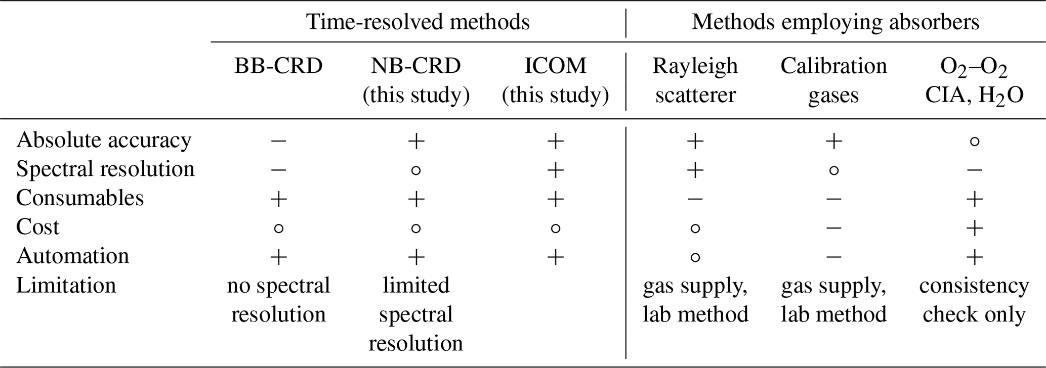
Table 1Strengths (+), limitations (−), and adequate sufficiency (∘) of current methods for the path length determination in optical resonators. CIA denotes collision-induced absorption.
2.1 Time-resolved methods
-
Broad-band cavity ring-down (BB-CRD). In cavity ring-down (CRD) spectroscopy, the decay of light intensity leaving the cavity is monitored for a modulated light source. In the simplest case, a monochromatic laser is used together with a fast photodetector, commonly a photomultiplier (O'Keefe and Deacon, 1988). Path length information is only retrieved at the laser wavelength. When broad-band light sources are used instead (broad-band CRD, BB-CRD), a multi-exponential decay in the signal is observed, as spectrally differently populated path lengths are superposed (Ball and Jones, 2003; Meinen et al., 2010). The spectral information of L(λ) is concealed and cannot be reconstructed without further assumptions.
-
Narrow-band cavity ring-down (NB-CRD). We present here a further development of the CRD method that also determines spectral information of the mirror reflectance by combining broad light sources with tunable narrow-band filters. NB-CRD is described in detail in Sect. 3.
-
Integrated calibration by means of optical modulation (ICOM). This study establishes ICOM as powerful new time-resolved method which adds only a little complexity. It is described in Sect. 4.
More time-resolved calibration methods exist (e.g. phase shift cavity ring-down spectroscopy (PSCRDS) – Engeln et al., 1996; Langridge et al., 2008; high-frequency clocked 2D spectrometers – Ball and Jones, 2003), which are however prohibitively expensive and not suitable as a mere calibration technique. PSCRDS employs a modulated light source (typically direct modulation of an LED, pulse length a few tens of nanoseconds) and a fast detector (photomultiplier tube, PMT). Spectral information is gained with a monochromator. The temporal evolution at the selected wavelength is sampled with a phase-sensitive lock-in amplifier. The measured phase shift readily determines the intra-cavity photon lifetime. PSCRDS therefore differs from ICOM in both the hardware and the analysis approach.
2.2 Methods employing absorbers
Other than time-resolved calibration methods, absorber-using calibration methods exploit the fact that the optical properties of gas in the measurement cell affect the transmission through the cavity. Operating the light source continuously at a constant intensity, slow dispersive detectors (spectrometers) can be used to retrieve spectral information. The extinction in the resonator can be adjusted by introducing gases exhibiting suitable absorption and scattering properties (Rayleigh and Mie) or an antireflection-coated optical substrate of known loss (Varma et al., 2009). The challenge is to accurately control cavity extinction properties, i.e. to introduce adequately strong absorbers or scatterers at accurate concentrations. An inherent problem of all absorber-using calibration techniques is low sensitivity at short path lengths, i.e. when the light attenuation is small. Additionally, intensity fluctuations of the light source can affect the retrieved path length if the total absorption instead of the differential absorption is used.
The most popular absorber calibration methods are the following:
-
Rayleigh scatterer. One can determine the setup properties by comparing gases of known and distinct Rayleigh scattering coefficient, e.g. helium and zero air (Washenfelder et al., 2008). Helium scatters less than air, such that more light passes to the spectrometer. In the case of zero air, O2–O2 collision-induced absorption needs to be considered as well. This method is relatively cheap but difficult to apply in the field: the handling and supply of gas during field campaigns (in particular aircraft campaigns) are critical. The complete purging of the measurement cell can be hard, both to accomplish and to verify. This method relies on a stable light source and transfer optics.
-
Calibration gases. Absorbing gases imprint their characteristic (differential) absorption signature on the retrieved spectrum. The spectral shape of the path length can be derived from the relative strength of the individual absorption structures. If the absorber is introduced at a known concentration, even an absolute path length retrieval is possible (Thalman and Volkamer, 2013). However, many relevant calibration gases (e.g. NO2, SO2) are toxic, are not stable and require on-site production; they might not cover the full wavelength range, or the accuracy of literature cross-sections are insufficient.
-
O2–O2 CIA, H2O. O2–O2 collision-induced absorption (CIA) occurs correlated to the concentration of oxygen in the entire UV–Vis spectral range (Finkenzeller and Volkamer, 2022) and can be predicted accurately if the air temperature, pressure, and humidity are known. As such, oxygen is a ubiquitous calibration gas (Platt et al., 2009; Thalman and Volkamer, 2013). However, the density of differential absorption features is insufficient to spectrally characterise the path length. Oxygen can only be used as a consistency check. Similarly, the absorption due to water can be compared to parallel measurements to check for consistency. For water, strong absorption in narrow absorption lines that are not resolved by typical spectrometers can lead to apparent non-Beer–Lambert behaviour, and special care may be required in the interpretation (Langridge et al., 2008).
While the above methods work in principle, they substantially complicate the use of optical resonators and either are difficult to implement or do not allow us to accurately retrieve the path length with spectral resolution and coverage. Here, we present two new methods: (1) integrated calibration by means of optical modulation (ICOM), which enables a high accuracy with spectral resolution and coverage in a relatively simple setup, easing the hitherto efforts needed in calibration. (2) We also present a closer look at the narrow-band cavity ring-down (NB-CRD) method.
3.1 Method description
The extension of the cavity ring-down method allows the retrieval of wavelength-dependent path length information by placing a wavelength-discriminating element in the instrument's light path. Ideally, the transmitted wavelength window should be tunable over the full range of wavelengths. One convenient, simple, and robust solution is to exploit the sensitivity of interference band-pass filters to the light incidence angle. The higher the incidence angle, the shorter the centre wavelength of the transmitted light (Fig. 1; Pollack, 1966). At the same time, the transmission peak is slightly broadened and the peak transmission is reduced. The maximum tilt angle is determined geometrically, when the effective section of the filter (perpendicular to the incident light) becomes smaller than the beam diameter. Typically, the usable wavelength range is on the order of 30 nm or 10 % of the centre wavelength. This approximately matches typical bandwidths of high-reflectivity mirrors and allows spectrally complete path length information for optimal mirror–filter combinations. The spectral tuning range could be extended by using multiple interference filters.
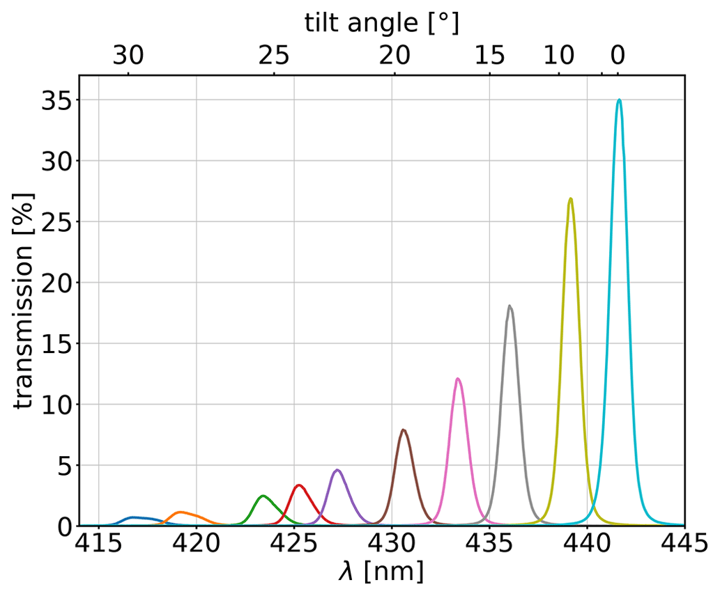
Figure 1Tilt angle sensitivity of transmission characteristics of interference band-pass filter with 441.6 nm nominal centre wavelength. Measured transmission curves are shown for tilt angles from 0∘ (orthogonal, 441.6 nm centre wavelength) to 30∘.
3.2 Instrument implementation
Figure 2 shows a schematic of the instrumental setup including an NB-CRD system. To record ring-down curves, a mirror is introduced into the light path, directing the light exiting the resonator onto a PMT (Hamamatsu H6780-01). The PMT signal is amplified by a custom three-stage amplifier and analysed by a small USB oscilloscope (PicoScope 2204). The highest sensitivity of the utilised PMT is at 400 nm. A Schott BG25 band-pass filter directly in front of the PMT blocks light with wavelengths longer than 470 nm. The interference filter used in this study (LOT-Oriel 442FS02-50) has a nominal centre wavelength of 441.6 nm at a nominal full width at half maximum of 1.0 nm. The LED feeding the resonator can be switched from the usual constant current operation into a pulsed mode using custom circuitry, in which it is turned on and off with a frequency of 8.7 kHz. A LabVIEW interface is used to control the tilt angle of the filter, record the ring-down signal from the oscilloscope, average data, fit the model function, and save the results.
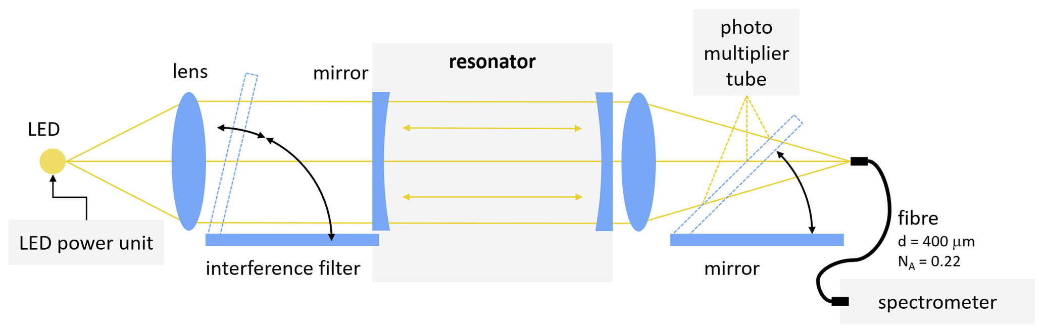
Figure 2Schematic of the CE-DOAS instrument assembly fitted for NB-CRD calibration. For spectrally resolved ring-down measurements, the interference filter can be driven into the light path under different angles. A mirror is used to deflect the beam into a photomultiplier tube.
3.3 Calibration routine
Path length calibration using NB-CRD is performed as follows. First, by acquiring spectra under constant illumination and different filter angles, the spectrometer wavelength calibration is used to determine the angle-specific centre transmission wavelength. Then, the LED is switched to pulsed operation and, for each selected filter angle, i.e. wavelength, ring-down signals are recorded with the PMT, of which 1000 are averaged. The path length is determined from an exponential fit to the ring-down signal. Usually, three sets are taken for each position to determine their standard deviation as a measure of precision. The wavelength-resolved calibration curve is derived by fitting a polynomial to wavelength-mapped data points. Depending on the number of sampling points and ring-down measurement sets per point, a calibration L(λ) takes between 30 and 60 min.
The temporal behaviour of systems is commonly sampled with detectors that allow exposure times TE significantly shorter than the characteristic setup timescales τ (Fig. 3a). Spectrometers used in CE-DOAS applications commonly have minimum exposure times of a few milliseconds, much longer than typical decay times of few microseconds. In ICOM, the time resolution of the spectrometer is effectively enhanced to the time resolution of an optical modulator added between the resonator and the spectrometer.
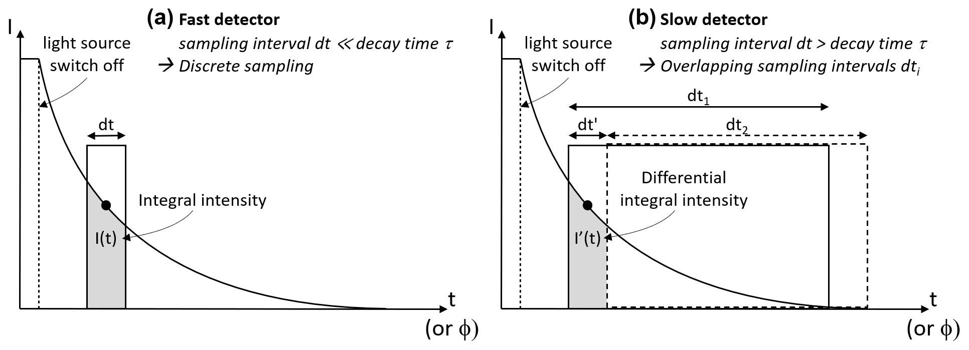
Figure 3Sampling of temporal evolution using fast and slow detectors. In conventional sampling (a), a fast detector with a sampling interval shorter than the characteristic time constant allows us to sample the temporal evolution point by point. If slow detectors are used (b), the same information can be retrieved by comparing overlapping sampling intervals.
Figure 4 illustrates the microscopic principle of ICOM, i.e. the evolution of physical parameters during individual cycles.
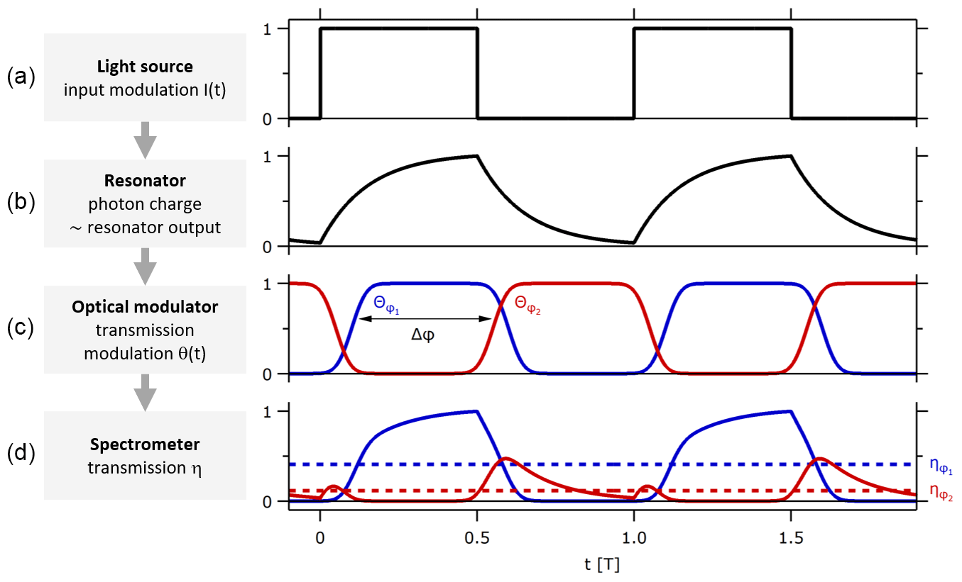
Figure 4Temporal evolution of physical properties in apparatus within two exemplary pulse cycles: (a) light input I(t) from the light source, (b) photon population in the resonator or output towards the spectrometer, (c) transmission θ(t) of the optical modulator for two exemplary phases, and (d) instantaneous (solid) and apparent (dashed) transmission η to the detector. The apparent transmission η is a function of the phase ϕ, τ, I(t), θ(t), and the modulation frequency ν.
The light source is operated in a modulated mode (pulsed) with period T and delivers an intensity I(t) (Fig. 4a). The photon population in the resonator changes correspondingly to the light input; the temporal evolution of the population, i.e. the shape of rise and decay, is determined by the decay time τ(λ). Photons are lost from the resonator by scattering, absorption, or transmission through the mirrors (Fig. 4b). The transmission θ(t) of the optical modulator between the resonator and the spectrometer oscillates between blocking and transmission of the light, with the same frequency ν as the light source and with a distinct, adjustable phase relation ϕ to the light input signal (Fig. 4c). The intensity reaching the spectrometer is the product of unblocked output (proportional to the photon population in the resonator) and transmission. The spectrometer does not resolve the instantaneous intensity but rather integrates the arriving photons over many pulse cycles (dashed lines in Fig. 4d). We refer to the averaged ratio of light intensity reaching the modulator and leaving the modulator (being transmitted) as apparent transmission η:
Critically for the ICOM idea, η is a function of decay time τ, i.e. path length L. It also depends on the phase ϕ, modulation frequency ν, and the direct and indirect modulation profile I and Θ. Using the modulation profiles I and Θ of the prototype employed in this study (Sect. 5.1), η is given in Fig. 5.
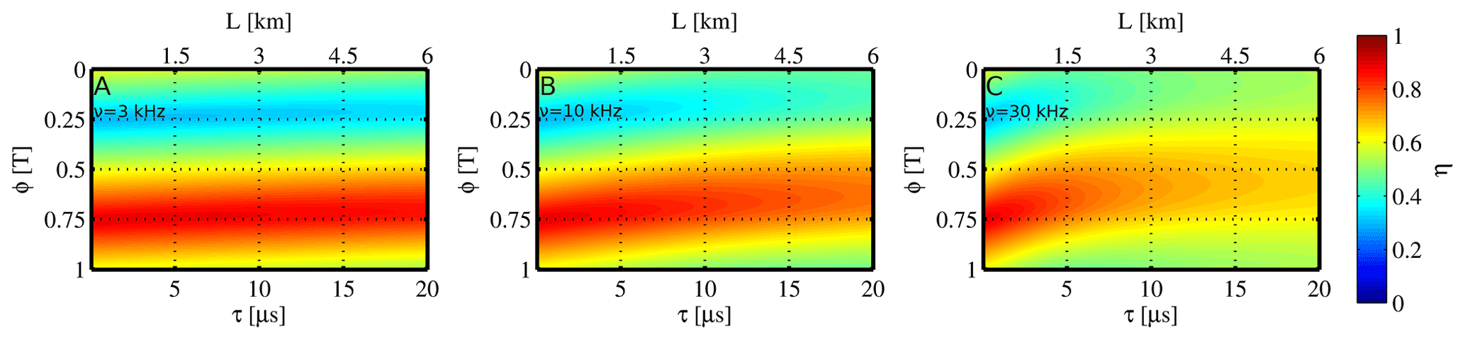
Figure 5Apparent transmission (colour-coded) of the demonstration setup (Sect. 5.1, quasi-rectangular I(t) and Θ(t) profile), modelled for three different modulation frequencies ν. The characteristic landscape of η(τ,ϕ) can be used to retrieve the path length.
Notably, even when the light source and the modulator are operated at a modulation frequency ν considerably slower than the corresponding decay times τ (approximately 1 order of magnitude), sufficient sensitivities for the determination of the path length can be achieved. This is clear in Fig. 3, as the intensity is still retrieved from a differential measurement. Even for modulators with non-rectangular transmission profiles, the temporal behaviour can be exploited, as long as the transmission profiles are characterised.
4.1 Shutter ratio and light pulse width
The pattern of both the direct modulation I(t) (of the light source) and the indirect modulation θ(t) (of the optical modulator) can be adapted to maximise the sensitivity for the retrieval of the path length. If the shutter transmitted only during a very narrow, i.e. short, time window and otherwise blocked the light (mean transmission -like transmittance), the exponential decay could be well explored point by point, without any broadening of the curve. However, at the same time, very little light would be transmitted to the spectrometer, resulting in a poor signal-to-noise ratio (or long measurement times). In the other extreme case, light throughput could be maximised with continuous transmission (), but all temporal information would be lost. Our simulations suggest that – depending on the expected path length range – best sensitivities S (Sect. 4.3) are achieved for a shutter ratio (i.e. 30 % mean transmission for a quasi-rectangular temporal transmission profile θ(t)) and a rectangular light pulse width of ∼50 %. The data presented in this study are based on the instrumental setup used (Sect. 5.1), where a slit wheel as a modulator with 50 % transmittance and an LED with a 50 % duty cycle were applied. This way, approximately 80 % of the potential sensitivity of ICOM to the determination of L(λ) is exploited.
4.2 Operation mode: single-shot mode and phase sweep mode
There are two modes in ICOM to determine the path length which are depicted in Fig. 6.
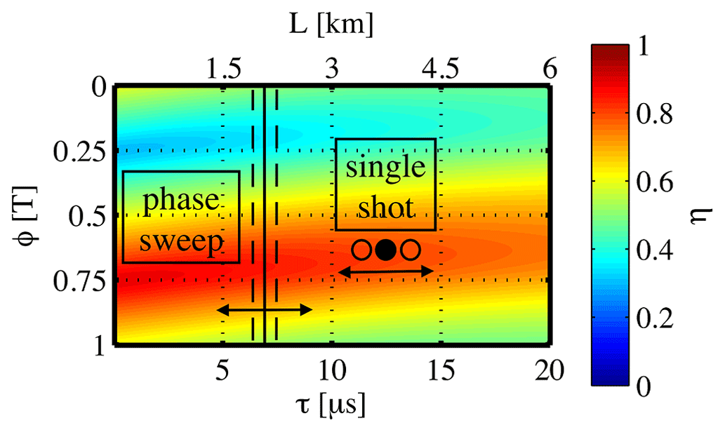
Figure 6Illustration of the two ICOM operation modes. Phase sweep mode: the apparent transmission η (Eq. 4) is measured at a quasi-continuous set of phases. The acquired ηMeas(ϕ) curve is then fitted into the modelled ηMod(ϕ,τ) landscape to retrieve the path length. Single-shot mode: the apparent transmission η is sampled at a fixed phase ϕ0. The acquired η(ϕ0) is then fitted to a modelled η(ϕ0,τ) curve to retrieve the path length.
-
The simplest approach to determine τ(λ) would be to set the phase relation ϕ between I(t) and θ(t) to a fixed value ϕ0, where is high (Eq. 5, Fig. 5, single-shot mode). η(ϕ0) could be determined as the ratio of the intensity measured once with an operational optical modulator to that measured once with a permanently transmitting modulator. τ can be determined as η(ϕ0) is a function thereof. This approach relies on the comparison of two intensities and is therefore susceptible to drifts in light input intensity and transmission of transfer optics and to offsets of ϕ0.
-
A more robust interpretation of η is readily possible if the phase is swept quasi-continuously (phase sweep mode). This way, an η(ϕ) spectrum is acquired, whose characteristic shape can be used for the path length retrieval. The absolute intensity is not relevant. The variation in the η(ϕ) spectra for different decay times is visualised in Fig. 7 for different modulation frequencies.
In evaluation, measured transmission spectra ηMeas(ϕ) are compared to modelled transmission spectra ηMod(τ,ϕ).

Figure 7Apparent transmission , as defined in Eq. (4), of the demonstration setup (Sect. 5.1, quasi-rectangular I(t) and Θ(t) profile), for three different modulation frequencies ν. Both the variable shape and the position of the extrema can be exploited for the retrieval of L(λ). Sufficient modulation frequencies ν are necessary for reasonable sensitivity.
4.3 Theoretical precision of the idealised ICOM setup
The precision of the phase modulation ICOM approach is determined by how precisely the shape of η(ϕ) can be measured and how much the shape of η(ϕ,τ) varies with changes in τ. For a specific phase ϕ, we define the single-shot sensitivity S′ as the relative change in the transmission η for small relative changes in τ:
Its dependency on ϕ and τ is visualised in Fig. 8.
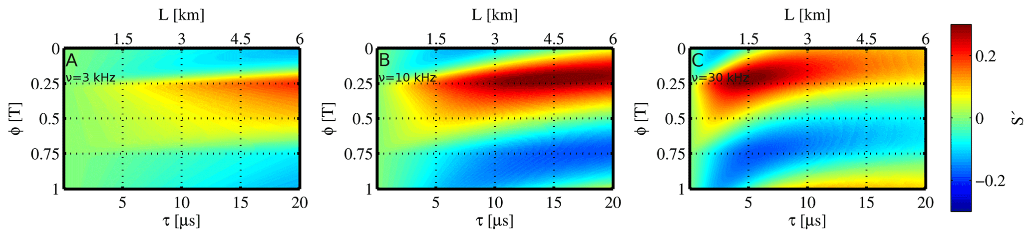
Figure 8Single-shot sensitivity (colour-coded) of the demonstration setup (Sect. 5.1, quasi-rectangular I(t) and Θ(t) profile), for three different modulation frequencies ν. Fields of high indicate where ICOM is sensitive to retrieving L.
In phase modulation mode, a set of n transmissions at different phases ϕi is acquired: . For the analysis of this case we define the sensitivity S for relative changes in τ:
where σ denotes the standard deviation. The standard deviation mathematically reduces information from the set of individual sampling points into one scalar and is (amongst possible others) a measure for how much the transmission curve changes with changing τ. One feature of the standard deviation exploited here is that a uniform scaling between two curves (e.g. two curves differ only by a constant scaling factor as a result of intensity drift in light source intensity) does not affect S, whereas a change in the shape of (i.e. there is a non-trivial transformation between two curves) does contribute to S.
It turns out that for our demonstration setup with rectangular light profile I(t) and quasi-rectangular transmission profile Θ(t), a modulation frequency ν=10 kHz yields a sensitivity S≥0.1 for decay times larger than 5 µs (Fig. 9). Faster modulation frequencies allow higher sensitivities at short path lengths and vice versa.
Starting from S≥0.1, we can estimate the precision in L in measurements, not taking into account systematic errors however. Let the precision of the individual transmission (intensity) measurement at the detector (e.g. one spectrometer channel) be a typical value of about
Then, the assumption (Eq. 7) and S≥0.1 in Eq. (6) yield the relative statistical uncertainty in path length:
The phase space does not need to be sampled with constant increments of ϕ. Selected sampling of the transmission curve η(τ,ϕ) at phases of high information content could enhance the precision of the method. However, in this study only equidistantly distributed phase series were considered.
In the following we discuss the practical realisation of an instrument based on the theoretical considerations and model calculations presented above.
5.1 Demonstration setup
The schematic description of the resonator and components used in the demonstration setup is given in Fig. 10.
The optical modulator Thorlabs MC2000 with 100-slot disc Thorlabs MC1F100 (transmission ratio 50 %) was used. Its electronic control unit allows the digital selection of modulation frequencies ν of up to 10 kHz. Its transistor–transistor logic (TTL) trigger output with selective delayed phase feeds the power supply unit of the light source (LED, Martin Anthofer, personal communication, 19 February 2015), generating a quasi-rectangular light pulse profile with a 50 % duty cycle.
In the standard CE-DOAS instrument a fibre of 400 µm diameter and a numerical aperture NA=0.22 is used to connect the resonator exit and the spectrometer assembly. This single fibre was split into two fibres, with the modulation optics in between. The exit of the first fibre is projected onto the plane of the slit wheel by a 1 in. plano-convex lens of 25 mm focal length. The object distance and image distance are 50 mm each, resulting in a unity magnification. After passing the chopper wheel, the image of the fibre is then projected by a second lens onto the fibre connected to the spectrometer.
An unfortunate artefact of the demonstration prototype is due to the fact that the electronic control unit used has two distinct operation regimes (phase , 90∘] and ϕ∈(90, 270∘)); i.e. at the transition a discontinuity in measured intensities appears. As a consequence, special care had to be taken to connect both regimes of ϕ.
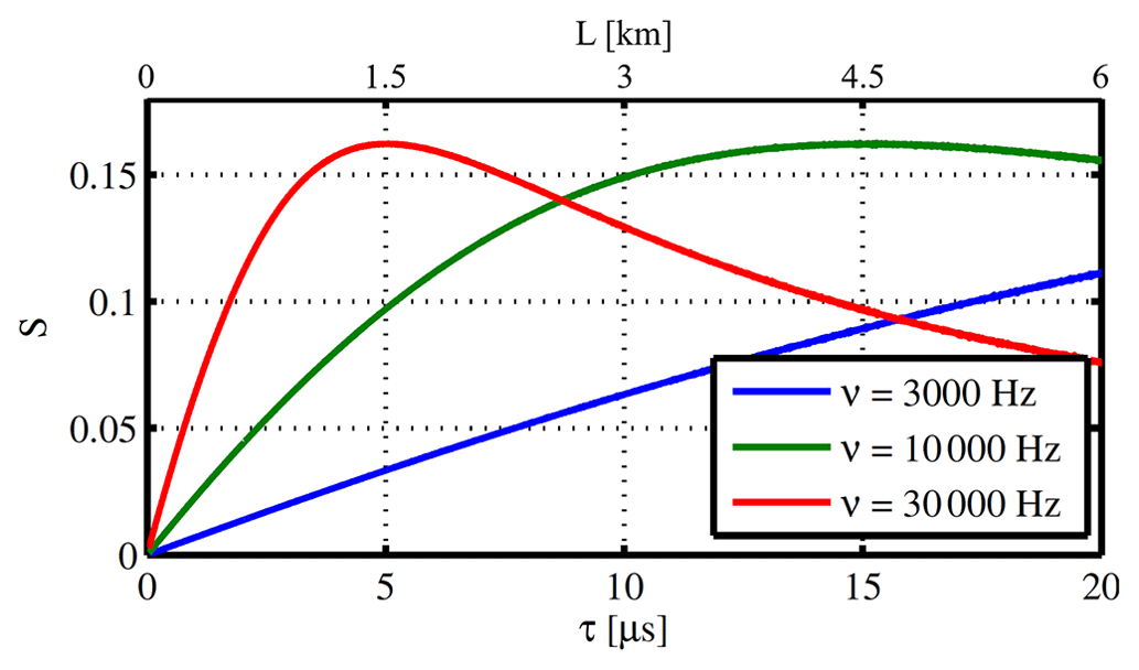
Figure 9Sensitivity S(τ) (Eq. 6) of the demonstration setup (Sect. 5.1, quasi-rectangular I(t) and Θ(t) profile) for three different modulation frequencies ν. At ν=3 kHz, S increases nearly linearly with decay time in the investigated path length range. At higher ν there are optimal sensitivities at certain decay times. ν should to be chosen accordingly to achieve maximum sensitivity S in the expected path length ranges.
5.2 Modelling of the apparent transmission η
The apparent transmission for k different values of τ (spanning the range of expected decay times) and the used set of ϕ is modelled numerically, using the laboratory-determined light pulse profile I(t) of the LED and the measured transmission profile θ(t) of the optical modulator. The respective profiles were recorded with a PIN photodiode and a transimpedance amplifier (Martin Anthofer, personal communication, 19 February 2015). The spacing between neighbouring ϕ values was 1∘ and 30 ns for τ (equivalent to 9 m), comparable to measurement noise. A look-up table of k spectra is generated for later comparison to measured data.

Figure 10Scheme of the experimental setup used in this study. The optical modulator is introduced in between the resonator (bottom) and the spectrometer.
Table 2Available optical modulators. ICOM demands modulation frequencies in the kilohertz range for fibre-sized beam diameters.
5.3 Data acquisition
Data were acquired with the software DOASIS (Kraus, 2006). It communicates with the spectrometer (Avantes AvaSpec ULS2048L-U2) and controls the phase ϕ. The modulation frequency ν of the optical modulator and of the LED was set to a constant value for a calibration run. As such, sets of measured spectra where were recorded. At typical integration times of 6 s, data acquisition requires approximately 40 min.
5.4 Data evaluation
The wavelengths λj of the individual spectrometer channels are evaluated separately. First, the data from the spectra are reordered channel-wise to yield phase spectra . Then, each measured phase spectrum is compared to modelled phase spectra of the previously generated look-up table using the Levenberg–Marquardt least-χ2 fitting algorithm:
Here, A and B are fit coefficients for the offset and scaling in intensity (to account for the pixel-dependent offset, dark current, offset in the shutter profile, and offset in the LED pulse profile); the constant phase offset ϕ0 is an instrument parameter. It can be determined either in auxiliary measurements or at wavelengths of known negligible path length. The root mean square (rms) of the fit residual is taken as a measure for the quality of the match. The phase spectrum with smallest rms identifies the most probable decay time, i.e. path length.
To account for the two distinct phase regimes of the specific chopper control unit used (discontinuity in the spectra at occurring in the instrumental setup used), the fitting scenario had to be extended by a box reference that allows different offsets in the two regimes:
Here, C is an additional fit coefficient accounting for the discontinuity.
6.1 Accuracy estimation: comparison of ICOM to NB-CRD and helium calibration
Figure 11 shows the comparison of retrieved wavelengths for an optical cavity in the blue wavelength range using ICOM, helium, and NB-CRD. The wavelength calibration of the spectrometer was performed using krypton emission lines.
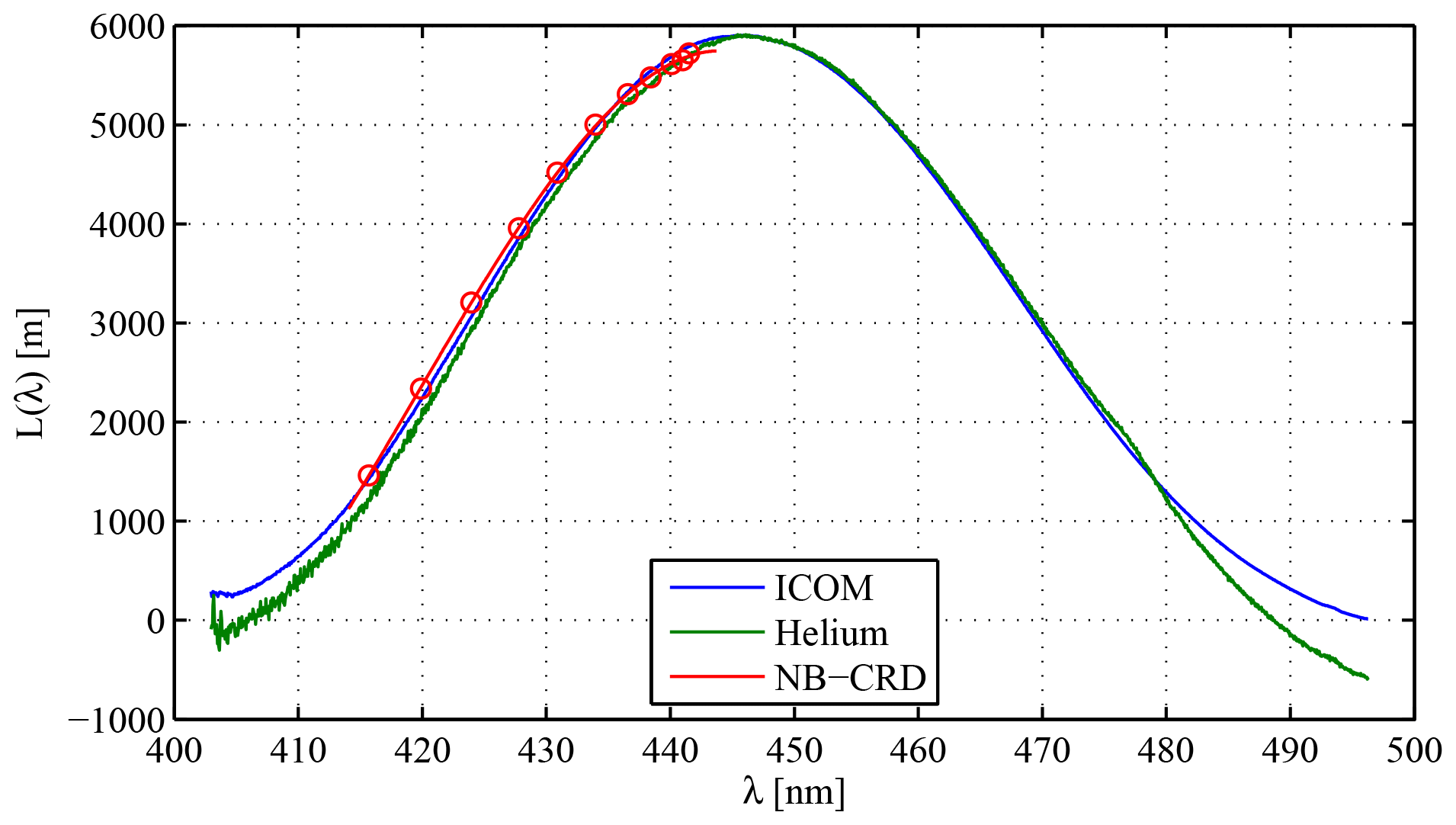
Figure 11Comparison of spectral path lengths retrieved with ICOM (blue line), helium (green line), and NB-CRD (red circles and line). The NB-CRD information is limited to λ≤442 nm, corresponding to the band-pass filter tuning range; the circles indicate the sampled wavelengths that were interpolated by a second-order polynomial. Significant differences only exist at the spectral margins, were the helium calibration determines non-physical negative path lengths.

Figure 12Demonstration of ICOM precision: deviation of five individually acquired Li values at ν=10 kHz from the mean path length . The variable noise in the spectrum is due to the spectrally non-homogeneous light intensity distribution. The path length assumes its maximum of ∼6 km at 443 nm (Fig. 11; ΔL=30 m corresponds to a relative difference of 0.5 %) and is essentially zero at the margins of the spectrometer range.

Figure 13Acquired intensity as function of phase ϕ and corresponding relative fit residual for modulation frequency ν=10 kHz. The congruence of modelled transmission and measured transmission is in the low percent range. The intensity spectra exhibit a discontinuity at ϕ=90 and 270∘ due to an instrumental artefact.
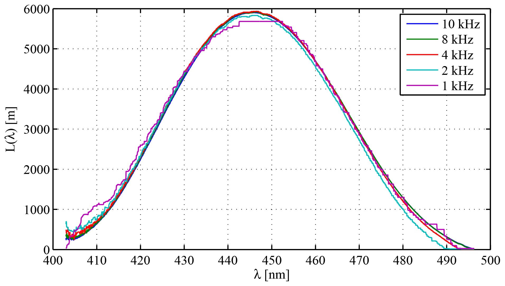
Figure 14Successful ICOM path length retrieval using artificially reduced modulation frequencies ν.
-
Helium calibration. The wavelength calibration of the spectrometer was performed using krypton emission lines. The measurement cell of the instrument was then purged with ambient air and helium repeatedly to verify complete flushing from reproducible intensity changes. Following the evaluation according to Washenfelder et al. (2008), the different amount of Rayleigh scattering between air and helium was used to derive the light path. The literature Rayleigh scattering cross-sections for helium and air (laboratory air passed through an active charcoal filter and drying cartridge to remove absorbing species and humidity) were calculated according to Thalman et al. (2014) and Bodhaine et al. (1999) (at λ=430 nm: , ); for the absorption cross-section of O2–O2 collision-induced absorption, data from Thalman and Volkamer (2013) were used (peak absorption at λ=446 nm: ). The resulting path length curve is included in Fig. 11.
Incomplete flushing of the resonator volume with helium can bias the path length short. Additionally, the exchange of the resonator gas bath by helium can alter the instrument illumination, compared to the illumination during measurements. This can bias the retrieved path length whether long or short (compare non-physical negative path lengths at 405 and 495 nm wavelength, Fig. 11). While the helium calibration achieves small statistical uncertainties of a few tens of metres (same order as noise on the curve), systematic errors due to incomplete flushing and drift in the light source intensity are likely much larger. Based on the derived non-physical negative path lengths, the accuracy of the helium-derived path length estimate is on the order of 300 m for the setup used, or 5 % of the peak path length.
-
Narrow-band CRD calibration. An NB-CRD calibration following Sect. 3 was performed for comparison. With the available filter, a path length retrieval for wavelengths longer than 442 nm was not possible. The ring-down signal was recorded at 11 different tilt angles. The individual L(λi) values were fitted by a second-order polynomial. L(λ) and the L(λi) values are included in Fig. 11. The accuracy of the NB-CRD path length estimate is comparable to the accuracy of the helium-derived path length estimate, i.e. on the order of 300 m, or 5 % of the peak path length.
The differently acquired L(λ) values (Fig. 11) show a good agreement for path lengths above a few kilometres with differences smaller than ∼100 m. Strikingly, the path length retrieved with helium calibration seems to be wavelength-shifted against the others. This could be due to inaccurate scattering cross-sections used in the helium calibration evaluation. It is difficult to specify the absolute accuracy of ICOM, as the comparison of both the NB-CRD and the helium calibration apparently does not exceed the accuracy of ICOM.
6.2 Precision estimation: repeated measurements
The precision of ICOM was assessed by five successive measurements of the path length of the same optical resonator, as in Sect. 6.1. The deviations of each path length from the mean path length are illustrated in Fig. 12. The five retrieved ICOM path lengths are very similar. The statistical uncertainty of the path length can be estimated from the channel-to-channel noise to be on the order of few 10 m for individual runs. A possible explanation for the systematical deviations of several tens of metres is a slightly shifting alignment of the optics, resulting in a shifting phase offset ϕ0. Electronic optical modulators would not be sensitive to such an effect. However, the reproducibility seems to be better than 50 m, independent of the absolute path length.
6.3 Agreement of modelled and measured data
Figure 13 shows the agreement between measured and modelled phase spectra from a single run at ν=10 kHz, consisting of statistical noise and systematic structures. The low noise, compared to the magnitude of systematic residual structures, demonstrates the high brightness of the ICOM approach, allowing swift and precise calibrations. The most relevant instrument interference in the demonstration prototype stems from the two distinct operation regimes of the phase control unit, creating discontinuities at ϕ=90 and 270∘. These are satisfactorily but not fully accounted for by the box reference included in the fit algorithm (Sect. 5.4), and should be no concern in future setups. We hypothesise that the residuals may arise partially due to jitter of the mechanical optical modulator, i.e. deviations from the average modulation θ(t) that lead to a distortion of modified apparent transmission η, and slight imperfections in the characterisation of I(t) and θ(t).
6.4 Required modulation frequencies
To investigate the minimum modulation frequency necessary for an accurate path length determination in our setup with a maximum path length of 6 km, the optical modulator was operated at reduced frequencies of , and 1 kHz. Figure 14 shows that the respective path lengths agree well down to ν≈ 2 kHz, where systematical differences start to appear. The path length for ν=1 kHz is non-physically coarsely step-shaped, suggesting numerical problems. However, ICOM appears to be also applicable for modulation frequencies in the low kHz range that are accessible by slower modulators.
6.5 Applicable optical modulators
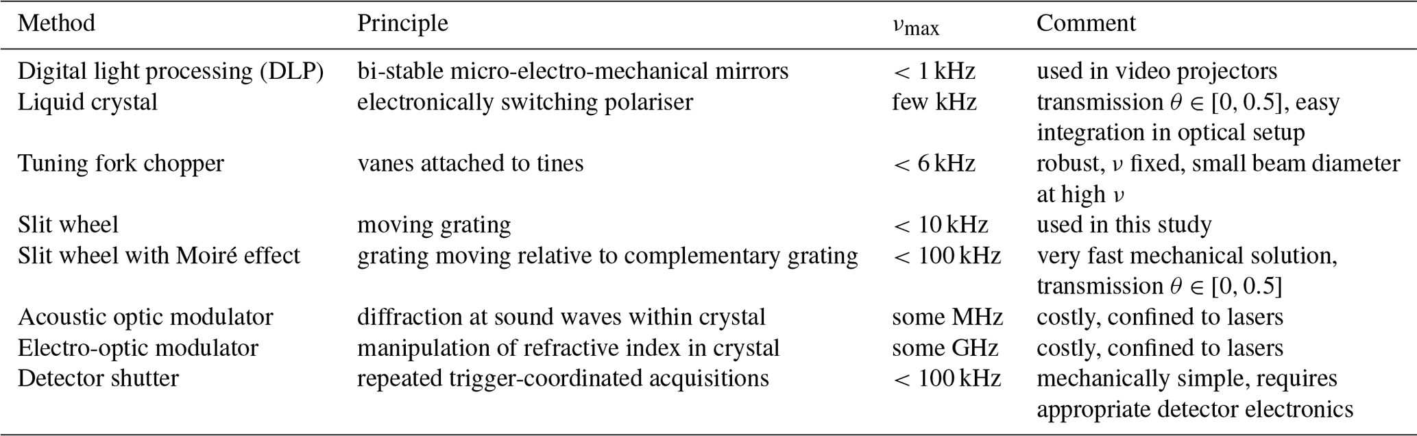
ICOM requires optical modulators that operate at frequencies of several kilohertz to ensure sensitivity and that have an aperture comparable to the beam diameters (e.g. the fibre diameter 400 µm). A high contrast, i.e. a strong modulation, is desirable. A potential wavelength dependence of the modulation would need to be characterised and considered appropriately. Table 2 lists various types of devices for the indirect modulation of optical beams. For the proof of concept, a rotating slit wheel was used because of its easy implementation and high performance. Slit wheels exploiting the Moiré effect, where instead of a slit a grating is swept over by a complementary grating, allow even higher frequencies of several tens of kilohertz. Tuning fork choppers are extremely robust but limited by the small beam diameter they permit at high frequencies. Liquid crystal optical modulators are promising, as they avoid moving parts and are likely easy to integrate into optical setups. Their maximum modulation frequency of liquid crystal optical modulators is limited by the autonomous aligning of the crystals after removal of the electric field. Micro-electro-mechanical mirrors (digital light processing (DLP)) and acousto- and electro-optic modulators are less relevant because of their complexity and cost.
Even without an additional optical modulator, it is in principle possible to sample the temporal evolution of a resonator charge with comparably slow detectors (conventional spectrometers). Rather than continuously modulating the light input and measuring mean intensities at the detector, single modulations can be sampled as long as the shift between input modulation and acquisition can be controlled (Fig. 3). The challenge of this approach consists in appropriate timing control and an appropriate signal-to-noise ratio, especially when the processing of a spectrum (detector clearing, exposure, read-out) for later software averaging takes much longer than the resonator decay time τ. The benefit is its simplicity is that it does not require calibration-specific transfer optics.
The agreement of ICOM, helium, and NB-CRD calibrations demonstrates the feasibility of the two new methods. NB-CRD is a relatively simple method that requires few components (filter, servo, photodetector, electronics) and yields robust path length measurements independent of consumables. With servo-actuated mirrors and filters, calibrations can be automated. The main challenge consists in achieving full spectral coverage by using band-pass filters matched to the spectral range. In ICOM, the path length in the resonator was determined with excellent statistical uncertainty of ∼10 m at the spectral resolution of the spectrometer, independently of the absolute path length. For typical multi-kilometre path lengths, this figure translates into a relative error in L well below 1 %. We show that ICOM also allows the accurate path length determination at modulation frequencies of few kilohertz that are accessible by optical modulators that avoid complexity and consumables. Advantages of ICOM are the high spectral resolution of the spectrometer (as during actual measurements), the high accuracy in path length, and the method's cost-efficient and robust design without consumables and wear objects (e.g. if a tuning fork chopper is used or if single modulations are sampled, Sect. 6.5). ICOM is an integrated calibration; i.e. even during calibration, spectral data are acquired that could be used to retrieve trace gas concentrations. The performance of ICOM can still be enhanced through the optimisation of control parameters. The combination of high performance and easy implementation makes ICOM and NB-CRD promising techniques for the spectral path length calibration of optical resonators, where other techniques are not feasible, e.g. in the field or in open-path setups.
The program code underlying this study is unfortunately no longer available due to a ransom-ware attack.
The raw and figure data underlying this study are unfortunately no longer available due to a ransom-ware attack.
UP, DP and MH developed the idea of NBCRD. MH implemented the respective setup. HF developed the idea of ICOM and, with the help from all co-authors, conducted the experiments and wrote the manuscript.
At least one of the (co-)authors is a member of the editorial board of Atmospheric Measurement Techniques. The peer-review process was guided by an independent editor, and the authors also have no other competing interests to declare.
Publisher’s note: Copernicus Publications remains neutral with regard to jurisdictional claims in published maps and institutional affiliations.
This research has been supported by the Deutsche Forschungsgemeinschaft within the funding programme “Open Access Publikationskosten” as well as by Heidelberg University.
This paper was edited by Hendrik Fuchs and reviewed by two anonymous referees.
Ball, S. M. and Jones, R.: Broad-Band Cavity Ring-Down Spectroscopy, Chem. Rev., 103, 5239–5262, 2003. a, b
Berden, G. and Engeln, R.: Cavity ring-down spectroscopy: techniques and applications, John Wiley & Sons, ISBN 978-1-4051-7688-0, 323 pp., 2009. a
Bodhaine, B. A., Wood, N. B., Dutton, E. G., and Slusser, J. R.: On Rayleigh optical depth calculations, J. Atmos. Ocean. Technol., 16, 1854–1861, 1999. a
Engeln, R., von Helden, G., Berden, G., and Meijer, G.: Phase shift cavity ring down absorption spectroscopy, Chem. Phys. Lett., 262, 105–109, https://doi.org/10.1016/0009-2614(96)01048-2, 1996. a
Fiedler, S. E., Hese, A., and Ruth, A. A.: Incoherent broad-band cavity-enhanced absorption spectroscopy, Chem. Phys. Lett., 371, 284–294, https://doi.org/10.1016/S0009-2614(03)00263-X, 2003. a
Fiedler, S. E., Hese, A., and Heitmann, U.: Influence of the cavity parameters on the output intensity in incoherent broadband cavity-enhanced absorption spectroscopy, Rev. Sci. Instrum., 78, 73104, https://doi.org/10.1063/1.2752608, 2007. a
Finkenzeller, H. and Volkamer, R.: O2–O2 CIA in the gas phase: Cross-section of weak bands, and continuum absorption between 297–500 nm, J. Quant. Spectrosc. Rad. Transf., 279, 108 063, https://doi.org/10.1016/j.jqsrt.2021.108063, 2022. a
He, Q., Fang, Z., Shoshanim, O., Brown, S. S., and Rudich, Y.: Scattering and absorption cross sections of atmospheric gases in the ultraviolet–visible wavelength range (307–725 nm), Atmos. Chem. Phys., 21, 14927–14940, https://doi.org/10.5194/acp-21-14927-2021, 2021. a
Herriott, D. R. and Schulte, H. J.: Folded Optical Delay Lines, Appl. Opt., 4, 883–889, https://doi.org/10.1364/AO.4.000883, 1965. a
Horbanski, M., Pöhler, D., Lampel, J., and Platt, U.: The ICAD (iterative cavity-enhanced DOAS) method, Atmos. Meas. Tech., 12, 3365–3381, https://doi.org/10.5194/amt-12-3365-2019, 2019. a
Kraus, S.: DOASIS – A Framework Design for DOAS, Shaker, ISBN 978-3832254520, 162 pp., 2006. a
Langridge, J. M., Ball, S. M., Shillings, A. J. L., and Jones, R. L.: A broadband absorption spectrometer using light emitting diodes for ultrasensitive, in situ trace gas detection, Rev. Sci. Instrum., 79, 123110, https://doi.org/10.1063/1.3046282, 2008. a, b
Meinen, J., Thieser, J., Platt, U., and Leisner, T.: Technical Note: Using a high finesse optical resonator to provide a long light path for differential optical absorption spectroscopy: CE-DOAS, Atmos. Chem. Phys., 10, 3901–3914, https://doi.org/10.5194/acp-10-3901-2010, 2010. a
O'Keefe, A. and Deacon, D. A. G.: Cavity ring-down optical spectrometer for absorption measurements using pulsed laser sources, Rev. Sci. Instrum., 59, 2544–2551, 1988. a, b
Pfund, A. H.: Atmospheric contamination, Science, 80, 326–327, 1939. a
Platt, U. and Stutz, J.: Differential Optical Absorption Spectroscopy; Principles and Applications, Physics of Earth and Space Environments, Springer-Verlag Berlin Heidelberg, https://doi.org/10.1007/978-3-540-75776-4, ISBN 978-3-540-21193-8, 2008. a
Platt, U., Meinen, J., Pöhler, D., and Leisner, T.: Broadband Cavity Enhanced Differential Optical Absorption Spectroscopy (CE-DOAS) – applicability and corrections, Atmos. Meas. Tech., 2, 713–723, https://doi.org/10.5194/amt-2-713-2009, 2009. a, b, c
Pollack, S. A.: Angular dependence of transmission characteristics of interference filters and application to a tunable fluorometer, Appl. Opt., 5, 1749–1756, 1966. a
Tang, K., Qin, M., Fang, W., Duan, J., Meng, F., Ye, K., Zhang, H., Xie, P., He, Y., Xu, W., Liu, J., and Liu, W.: Simultaneous detection of atmospheric HONO and NO2 utilising an IBBCEAS system based on an iterative algorithm, Atmos. Meas. Tech., 13, 6487–6499, https://doi.org/10.5194/amt-13-6487-2020, 2020. a
Thalman, R. and Volkamer, R.: Inherent calibration of a blue LED-CE-DOAS instrument to measure iodine oxide, glyoxal, methyl glyoxal, nitrogen dioxide, water vapour and aerosol extinction in open cavity mode, Atmos. Meas. Tech., 3, 1797–1814, https://doi.org/10.5194/amt-3-1797-2010, 2010. a
Thalman, R. and Volkamer, R.: Temperature dependent absorption cross-sections of O2-O2 collision pairs between 340 and 630 nm and at atmospherically relevant pressure., Phys. Chem. Chem. Phys., 15, 15371–15381, https://doi.org/10.1039/c3cp50968k, 2013. a, b, c
Thalman, R., Zarzana, K. J., Tolbert, M. A., and Volkamer, R.: Rayleigh scattering cross-section measurements of nitrogen, argon, oxygen and air, J. Quant. Spectrosc. Ra. Transf., 147, 171–177, https://doi.org/10.1016/j.jqsrt.2014.05.030, 2014. a
Thoma, M. L., Kaschow, R., and Hindelang, F. J.: A multiple-reflection cell suited for absorption measurements in shock tubes, Shock Waves, 4, 51–53, https://doi.org/10.1007/BF01414633, 1994. a
Varma, R. M., Venables, D. S., Ruth, A. A., Heitmann, U., Schlosser, E., and Dixneuf, S.: Long optical cavities for open-path monitoring of atmospheric trace gases and aerosol extinction, Appl. Opt., 48, B159–B171, https://doi.org/10.1364/AO.48.00B159, 2009. a
Wang, S., Schmidt, J. A., Baidar, S., Coburn, S., Dix, B., Koenig, T. K., Apel, E., Bowdalo, D., Campos, T. L., Eloranta, E. W., Evans, M. J., DiGangi, J. P., Zondlo, M. A., Gao, R.-S., Haggerty, J. A., Hall, S. R., Hornbrook, R. S., Jacob, D., Morley, B., Pierce, B., Reeves, M., Romashkin, P., ter Schure, A., and Volkamer, R.: Active and widespread halogen chemistry in the tropical and subtropical free troposphere, P. Natl. Acad. Sci. USA, 112, 9281–9286, https://doi.org/10.1073/pnas.1505142112, 2015. a
Washenfelder, R. A., Langford, A. O., Fuchs, H., and Brown, S. S.: Measurement of glyoxal using an incoherent broadband cavity enhanced absorption spectrometer, Atmos. Chem. Phys., 8, 7779–7793, https://doi.org/10.5194/acp-8-7779-2008, 2008. a, b
White, J. U.: Long Optical Paths of Large Aperture, J. Opt. Soc. Am., 32, 285–288, https://doi.org/10.1364/JOSA.32.000285, 1942. a
Zheng, K., Zheng, C., Zhang, Y., Wang, Y., and Tittel, F. K.: Review of Incoherent Broadband Cavity-Enhanced Absorption Spectroscopy (IBBCEAS) for Gas Sensing, Sensors, 18, 3646 pp., https://doi.org/10.3390/s18113646, 2018. a
Zhu, Y., Chan, K. L., Lam, Y. F., Horbanski, M., Pöhler, D., Boll, J., Lipkowitsch, I., Ye, S., and Wenig, M.: Analysis of spatial and temporal patterns of on-road NO2 concentrations in Hong Kong, Atmos. Meas. Tech., 11, 6719–6734, https://doi.org/10.5194/amt-11-6719-2018, 2018. a