the Creative Commons Attribution 4.0 License.
the Creative Commons Attribution 4.0 License.
 | 12 Jan 2023
Source apportionment of black carbon and combustion-related CO2 for the determination of source-specific emission factors
Balint Alfoldy
Asta Gregorič
Matic Ivančič
Irena Ježek
Martin Rigler
Black carbon (BC) aerosol typically has two major sources in the urban environment: traffic and domestic biomass burning, which has a significant contribution to urban air pollution during the heating season. Traffic emissions have been widely studied by both laboratory experiments (individual vehicle emission) and real-world measurement campaigns (fleet emission). However, emission information from biomass burning is limited, especially an insufficiency of experimental results from real-world studies. In this work, the black carbon burden in the urban atmosphere was apportioned to fossil fuel (FF) and biomass burning (BB) related components using the Aethalometer source apportionment model. Applying the BC source apportionment information, the combustion-related CO2 was apportioned by multilinear regression analysis, supposing that both CO2 components should be correlated with their corresponding BC component. The combination of the Aethalometer model with the multilinear regression analysis (AM-MLR) provided the source-specific emission ratios (ERs) as the slopes of the corresponding BC–CO2 regressions. Based on the ER values, the source-specific emission factors (EFs) were determined using the carbon content of the corresponding fuel. The analysis was carried out on a 3-month-long BC and CO2 dataset collected at three monitoring locations in Ljubljana, Slovenia, between December 2019 and March 2020. The measured mean site-specific concentration values were in the 3560–4830 ng m−3 and 458–472 ppm ranges for BC and CO2, respectively. The determined average EFs for BC were 0.39 and 0.16 g(kg fuel)−1 for traffic and biomass burning, respectively. It was also concluded that the traffic-related BC component dominates the black carbon concentration (55 %–64 % depending on the location), while heating has the major share in the combustion-related CO2 (53 %–62 % depending on the location). The method gave essential information on the source-specific emission factors of BC and CO2, enabling better characterization of urban anthropogenic emissions and the respective measures that may change the anthropogenic emission fingerprint.
- Article
(5819 KB) - Full-text XML
- BibTeX
- EndNote


Biomass burning (BB) is a significant source of black carbon (BC), brown carbon (BrC), and organic particulate matter, creating a contribution to climate change (Myhre et al., 2013; Tomlin, 2021) and a severe risk to human health (Naeher et al., 2007; Janssen et al., 2011; Sigsgaard et al., 2015; Chen et al., 2017; Brown et al., 2020; Karanasiou et al., 2021). Global hotspots of BB are associated with extensive and persistent wildfires (e.g., deliberate forest burning in Amazonia and Indonesia, accidental forest and savanna fires in central Africa, North America, the Mediterranean basin, and Siberia) (see, e.g., Val Martin et al., 2006; Giglio et al., 2013; Smirnov et al., 2015; Chiloane et al., 2017; Healy et al., 2019; Reddington et al., 2019). On the other hand, emission from domestic wood combustion for the purpose of space heating, water boiling, or cooking significantly contributes to the BB emission as well, especially in locations of high population density and reduced ventilation (Karagulian et al., 2015; Klimont et al., 2017; Mitchell et al., 2017).
Wood combustion is an important energy source, even in well-developed countries, where its emissions add to traffic-related air pollution. The share of wood combustion in the total European energy budget is expected to increase dramatically due to the current energy crisis that most European countries face nowadays.
The emission characteristics of BB differ from those of internal combustion of fossil fuel (FF), where the combustion is more complete. Consequently, FF combustion emits less CO, particulate matter, and organic compounds per unit of fuel mass while having higher NOX emissions compared to BB due to the higher combustion temperature and excess of air (see EEA, 2019: 1.A.3.b. versus 1.A.4.a–b.).
Black carbon is a dominant form of particulate matter emitted from fossil fuel combustion. Diesel engines (before the Euro 5 legislation standard) emit more than 80% of the particle mass (PM) as BC (EEA, 2019: 1.A.3.b.). Since diesel vehicles dominate the European vehicle fleet (Cooper, 2020), the high traffic-related BC emission poses significant air quality problems in cities, which is complemented by the BB emission during the heating season.
Due to their harmful health effects, BC emissions of diesel engines have been studied intensively worldwide for a long time (see the original work of Hansen and Rosen, 1990). The BC emission factors have been determined by numerous studies based on laboratory chassis dynamometer tests (Alves et al., 2015; Park et al., 2020) or real-world on-road measurements using either the chasing method (Wang et al., 2012; Ježek et al., 2015; Zavala et al., 2017) or on-board tailpipe measurements by the PEMS (Portable Emission Measurement System) (Zheng et al., 2015; Giechaskiel et al., 2019). These tests refer to the emission factors (EFs, emitted pollutant per kilogram of fuel or kilometer) of individual vehicles and do not reflect the emission of the entire vehicle fleet. By contrast, roadside monitoring offers the opportunity to measure a statistically significant number of vehicles. These measurements are usually carried out in tunnels (Sánches-Ccoyllo, 2005; Ban-Weiss et al., 2009; Brimblecombe et al., 2015; Blanco-Alegre et al., 2020), where elevated pollution concentration levels and negligible interference of other combustion sources (like wood burning) can be ensured. In these studies, the EF calculation is usually based on the carbon-balance method (Brimblecombe et al., 2015), when the plume CO2 increment is used to determine the burnt fuel mass.
In contrast, emissions from biomass burning are not controlled nearly as strictly as from mobile sources. Some studies have investigated specific combustion appliances, providing the emission factors of various pollutants (Querol, 2016; Nielsen et al., 2017; Holder et al., 2019; Trubetskaya et al., 2021). The advantages of these studies are the controlled experimental conditions, the information about the combustion parameters (fuel type, combustion temperature, excess of air), and the opportunity to change these parameters, and thus EFs concerning a wide spectrum of fuels and combustion conditions were reported. However, since only a limited number of stoves and combustion scenarios were studied, it is difficult to extrapolate these results to a “real-world situation” of a city.
For this reason, other papers focus on the real-world situation and report the atmospheric concentrations of the BB-related air pollution. However, since the contribution of the traffic emission always interferes, the pure BB-related air pollution is difficult to study. Consequently, some studies selected specific locations like Glojek et al. (2022) in Loški Potok, Slovenia, that can be considered a model village of biomass burning emission with a negligible contribution of other sources of air pollution. Other studies utilize the source apportionment model (Aethalometer model) of Sandradewi et al. (2008) and reported BB- and FF-related BC concentrations separately (see, e.g., Dumka et al., 2018; Deng et al., 2020; Liakakou et al., 2020; Mbengue et al., 2020; Milinković et al., 2021).
Despite the reliable source apportionment of BC by the Aethalometer model, the determination of the source-specific EFs in a real-world situation is still problematic due to the lack of the CO2 source apportionment. However, inverse modeling can offer the opportunity to trace back the air pollution to their sources. For example, Olivares et al. (2008) applied inverse modeling to retrieve the traffic- and BB-related emission factors of NOX, PM10, BC, and particle number.
In this paper we aimed to determine the biomass burning and traffic-specific BC emission factors in the urban atmosphere during the heating season. We used the carbon-balance method that required the simultaneous source apportionment of BC and CO2 concentrations. The BC source apportionment was performed by the Aethalometer model (AM), while the source apportionment of CO2 was implemented by multilinear regression analysis (MLR). After the source apportionment of both components, the specific emission ratios (ERs) for BB and FF were determined and converted to EF values following the carbon-balance method. The measurements were taken during a 3-month-long monitoring campaign in Ljubljana, Slovenia, during winter 2019–2020. The atmospheric concentration of black carbon was monitored with simultaneous CO2 measurement at three locations of the city with different emission characteristics involving traffic- and heating-related emissions as well as an urban background site.
In the following we introduce our combined Aethalometer model–multilinear regression analysis (AM-MLR) method that we applied for the determination of the source-specific emission factors. We present the BB- and FF-related emission factors for three different locations of the city. In order to validate the AM-MLR method, an auxiliary measurement campaign was performed during summer, when only fossil fuel combustion was assumed to be present. The FF-related emission factors determined during the summer campaign were compared to the result of the AM-MLR method.
2.1 Measurement sites and instrumentation
The measurement campaign took place from December 2019 to March 2020. Three measurement sites were selected in the city with different microenvironments, source profiles, and emission activities (Fig. 1). One location was selected in the historical center of the city (Trnovo, TRO), where wood combustion represents the primary energy source for domestic heating during winter. This site is located in the restricted traffic area of the old town, where low direct vehicle emission is expected. The measurement setup was installed in a family house, with the sampling inlet on the roof, 8 m above the ground, to ensure the access of air masses arriving from all directions.
Another location was selected close to major roads and far from biomass burning sources that ensured measurement of the higher relative contribution of traffic emission. The instruments were installed in a waterproof cabinet in the open recreational area of the Atlantis sport complex in the BTC commercial center (BTC site). Due to the open environment of the location, a 3 m sampling height was chosen.
The third measurement location was the atmospheric observatory of Aerosol d.o.o (Skylab, SKY) that is considered to be an urban background location. This location is far from the major roads of the city and is not affected directly either by traffic emission or wood combustion. The sampling inlet was at 10 m above the ground, which ensured free access of air masses from each direction.
The equivalent black carbon (eBC, referred to as BC in the following) concentrations were monitored using multi-wavelength Aethalometers (AE33, Magee Scientific/Aerosol d.o.o. Slovenia, Drinovec et al., 2015) that measure the light attenuation of the particle sample collected on a Teflon-coated glass filter tape (M8060) at seven wavelengths (370–950 nm). The absorption coefficient of the particle sample (babs, Mm−1) was obtained by dividing the attenuation coefficient by the multiple scattering parameter (C=1.39 for the M8060 filter tape; Weingartner et al., 2003; Yus-Díez et al., 2021). The BC mass concentrations were generated as the ratio of the absorption and the wavelength-dependent mass absorption cross-section parameter (MACλ, m2 g−1) provided by the manufacturer. Although the default MAC values cannot be used universally, their validity has been proven for Ljubljana (Ogrizek et al., 2022).
Aerosol size selection was provided at the inlet of the Aethalometer by a cyclone sampling head with a PM2.5 cut-off diameter. The flow rate was set to 5 L min−1 and the measurement time resolution to 1 min. The “dual-spot” technology enables the real-time loading effect correction, which is especially important when the spectral dependence of optical absorption is used for source apportionment (Drinovec et al., 2015).
The CO2 concentrations were measured by flow-through CO2 sensors (Carbocap GMP 343, Vaisala, Finland). The CO2 sensors were directly connected to the exhaust of the AE33, and thus they analyzed the identical air stream to the Aethalometer. The accuracy of the sensor was 3 ppm + 1 % of the reading below the 1000 ppm concentration range, which was the case during the campaign even on the most polluted days. The response time of the sensor was comparable with the AE33, so the 1 min average signals of BC and CO2 were well correlated when common sources were measured.
The three measurement systems were compared in the air quality laboratory of Aerosol d.o.o before the campaign. The variation between the AE33 units was below 1 % at 1 min averaging time for all the used wavelengths (880 nm for the BC concentration and 470 and 950 nm for the source apportionment). This precision was expected from the results of Cuesta-Mosquera et al. (2021), who compared 23 AE33 units and found variation between the measurement results of less than 1 %. The unit-to-unit variability of the CO2 sensors was below 4 ‰ on a 1 min time basis.
2.2 Meteorological situation
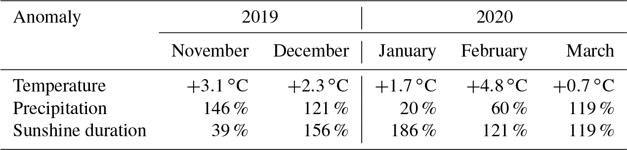
The measurement campaign started on 6 December 2019, during a warming-up period that was continued by an unusually warm and dry January and February (Fig. 2). Table 1 summarizes the basic climatological anomalies compared to the reference long-term averages of the 1981–2010 period. The average monthly temperatures in Ljubljana during the 3-month-long campaign were warmer than the long-term averages of the 1981–2010 period (2.3, 1.7, and 4.8 ∘C above the long-term average in December, January, and February, respectively). February 2020 was the second-warmest February in the history of measurements. Usually, January and February are the driest periods of the year, and in 2020, they were even drier than the average. The snow cover was negligible, limited to a few days during the measurement period.
Atmospheric dilution and dispersion significantly affect the pollution accumulation in the planetary boundary layer and play an essential role in the formation of the concentration level (Alfoldy and Steib, 2011). For the quantification of the dispersion of the pollution, the ventilation coefficient (VC, m2 s−1) as the product of the horizontal wind speed and the depth of the planetary boundary layer was applied. These parameters were provided by the Real-time Environmental Applications and Display System (READY) of the NOAA. The meteorological data used for the model calculations were obtained by the Global Data Assimilation System (GDAS), with a spatial resolution of 1 ∘ and a temporal resolution of 3 h.
The VC value for Ljubljana followed a lognormal distribution from 166 to 63 500 m2s−1 during the measurement period, with the median of the 2530 and 1460–4570 m2 s−1 interquartile range (see Fig. 3).
We identified the well-mixed, diluted cases based on high VC values, while low VC values referred to the opposite cases, when the atmospheric dispersion of the pollution was moderate, and thus emissions of local sources dominated the measured concentrations.
Table 1Monthly meteorological anomalies relative to reference long-term averages of the 1981–2010 period.
2.3 ER and EF calculation
Air pollution emission from combustion sources is usually reported with respect to burnt fuel mass and is given in a fuel-consumption-specific EF in g(kg fuel)−1. Although the combustion is never complete, more than 99 % of the fuel carbon content is oxidized to carbon dioxide (EEA, 2019) that can be used as a tracer for fuel consumption estimation. Dividing the pollution concentration increment by the CO2 increment of the plume, the pollution-to-CO2 ER can be determined.
The ratio of concentration increments in the plume can be calculated in an integrative or derivative way. If the time resolution of the measurement technique of the two components differs significantly, the two concentrations would not be correlated even if they have a common source. In this case, the integrative method is the preferable option for ER calculation. In this way the time integrals of the concentration peaks are calculated (peak area), and the ratio of the net peak areas (after background removal) provides the ER (see, e.g., Ježek et al., 2015). The disadvantage of this method is that the peak identification is arbitrary, and the background definition and removal burden the calculation with an additional uncertainty.
On the other hand, if the time resolution of the two measurement techniques is similar, the recorded pollutant concentrations originating from a common source are correlated in time. In this case a threshold value can be defined for the minimum required R2 of the correlation. Above the threshold R2 the two components are considered to originate from the same source (plume event), and the slope of regression provides the ER (derivative way). The offset of the regression line depends on the background concentrations that do not need to be taken into consideration during the calculation. This method also provides a well-defined plume event identification since the correlation between the two components is weak out of the plume, while a strong correlation indicates simultaneous concentration peaks of the two components.
In our case the 2 ER was calculated by the derivative method, and later it was transformed to EF using the carbon content of the concerned fuel:
where CC is the carbon content of the fuel that is 0.86 for diesel oil and petrol (Huss et al., 2013), while it ranges between 0.42 (eucalypt) and 0.47 (olive wood) when considering dry wood (Gonçalves et al., 2012). Here we applied the value of 0.45, which corresponds to the most usually used pine and oak wood. The measured CO2 concentration was converted from ppm to mg m−3 using a 1.82 mg m−3 ppm−1 conversion factor considering the AMCA (Air Movement and Control Association International Inc.) atmospheric standard (T=21.11 ∘C, P=1013.25 mbar) that was also applied by the Aethalometer for the BC concentration calculation. Molecular weights of CO2 (44) and C (12) were used to calculate the carbon mass fraction in CO2.
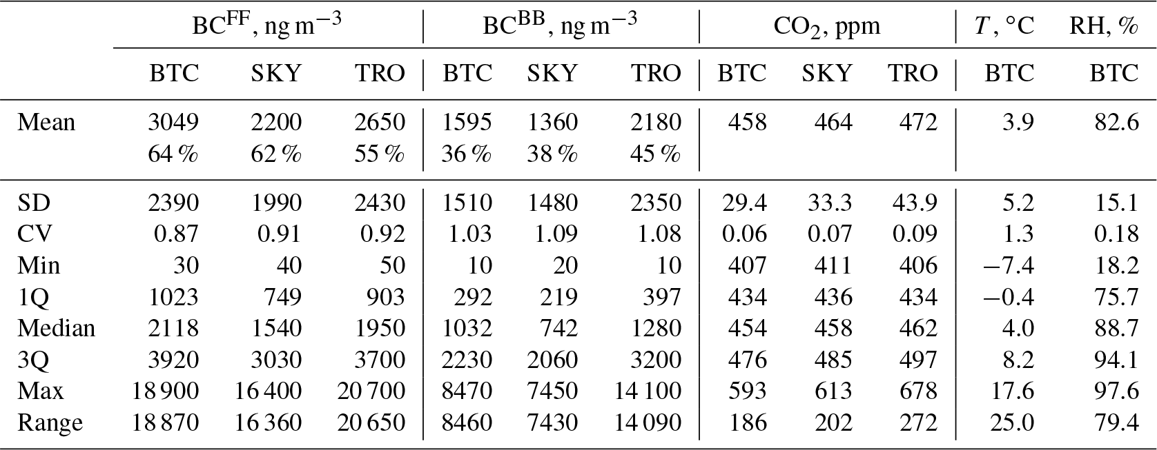
Table 2Statistical metrics of the measurements at the three monitoring locations. Mean (with the source-specific percental share with respect to the total BC), standard deviation (SD), their ratio (coefficient of variation, CV), the three quartiles (1Q, “Median”, 3Q), minimum and maximum values as well as their difference (“Range”) were calculated from the FF- and BB-related BC and CO2 concentrations. Statistical values for the temperature (T) and relative humidity (RH) were given as well for the BTC locations only.
2.4 Source apportionment and source-specific emission ratios
Measurement of the spectrally resolved absorption coefficient provides an insight into the composition of light-absorbing particles, allowing us to distinguish the highly (and widely) absorbing black carbon (soot) particles from brown carbon (light-absorbing organic aerosols; see Bond and Bergstorm, 2006; Drinovec et al., 2015). Fossil fuel combustion generates mostly pure soot particles that are strong light absorbers over the whole NIR-visible wavelength domain, while particles generated by biomass burning contain other light-absorbing compounds such as brown carbon that have characteristic absorbance bands in the near-UV domain (Sandradewi et al., 2008; Helin et al., 2018).
Sandradewi et al. (2008) developed the so-called “Aethalometer model”, where the absorptions at the 470 and 950 nm wavelengths were expressed as the sum of the absorptions of the FF- and BB-related BC components (BCFF and BCBB), while the ratios of the absorptions at different wavelengths follow a reciprocal power law of the wavelength ratio with a corresponding exponent (absorption Ångström exponent, AAE) of FF- or BB-related BC. In this study, an AAE of 1.15 was used for the FF-related emission whose value was determined during the summer auxiliary measurements when only FF sources were considered (see Sect. 2.5). For the BB-related component, an AAE of 2.1 was set according to the maximal AAE values that we measured at the TRO location (wood burning site) during nights when a low traffic contribution was assumed. The solution of the equation system results in the BB-related absorption at the 950 nm wavelength whose ratio to the total absorption provides the ratio of the BB-related BC concentration.
2.4.1 CO2 source apportionment
In order to apply the carbon-balance method for the source-specific EF calculation, source apportionment of the carbon dioxide is needed as well, which was implemented using the BC source apportionment combined with MLR. The method assumes that either the FF- or BB-related CO2 component is correlated with the corresponding BC component (BCFF or BCBB) in the plume. The total measured CO2 can be expressed as follows:
where CO and CO stand for the FF- and BB-related CO2 components of the plume, respectively, while CO represents the background concentration that changes much more slowly than the combustion-related components; thus, it can be considered constant during a plume event.
Equation (2) can be formulated using the FF- and BB-related BC concentrations and emission ratios (ERFF, ERBB),
or written in an equivalent form:
Equation (4) expresses that the linear combination of BCFF(t) and BCBB(t) is correlated with the measured CO2 using an appropriate ERFF/ERBB ratio. Our task is to find a particular ERFF/ERBB ratio which provides the best correlation between the two sides of Eq. (4). After the best correlation was found, the slope of the regression line provides 1/ERFF, so ERBB can also be calculated. The background CO2 concentration determines the offset of the regression and does not need to be taken into consideration during the calculation. However, the background CO2 provided by MLR is also valuable information that we present in this paper.
It has to be noted that oil burning for heating purposes is not usual in Ljubljana, so we could apportion all the FF-related BC to traffic sources. A high contribution of oil burning in the household energy production would interfere with the source apportionment that limits the applicability of the method in those locations, where oil heating is negligible.
The MLR analysis is a well-known and widely used method in source apportionment calculations; however, its combination with the Aethalometer model just recently appeared in the literature. Blanco-Alegre et al. (2022) applied the MLR method to decouple the BB- and coal-combustion-related BC based on source-specific correlations between specific tracers (K for wood burning and As for coal combustion).
Kalogridis et al. (2018) used the source apportionment information provided by the Aethalometer model for the source apportionment of carbon monoxide (CO) in Athens. They compared their result with the linear CO–NOX model (see there) and concluded that the CO–NOX model overestimates the BB-related CO contribution, maybe due to the photochemical loss of NOX, while the MLR analysis provided more reliable results.
Table 3Fitting parameters of the lognormal ER distributions (ng m−3 ppm−1) at the three locations of the city (see Fig. 5). The distributions are normalized to 1. The derived median and mean ER values are also shown.

The AM-MLR presented here can thus be a universal technique for source apportionment of any air pollution component that co-emitted with BC (for example, organic carbon, CO2, CO, NO, NO2, SO2, PM, or volatile organic compounds (VOCs).
For the application of the MLR analysis, the R statistical package “stats” (R Core Team, 2021) was used. The correlations were studied in a running time window with 1 h duration. During this time interval the background concentration is supposed to be constant, while the FF and BB sources have characteristic emission peaks.
The minimum R2 criterion for the MLR analysis was set to 0.9, which represents a good correlation between the source-specific BC and CO2 components. The correlation coefficient exceeded this threshold value during pronounced peak events only. A low R2 value means uncorrelated BC and CO2 peaks (i.e., shifted in time) or no presence of peaks in the time window. However, numerous BC peaks had to be discarded from the analysis due to the low or noisy CO2 peak that resulted in a lower correlation coefficient than the threshold (see more in Sect. 3.2).
It should be noted that, during the 1 h time window, several FF- and BB-related sources contribute to the measured plume with different ERs. The emitted BC and CO2 concentrations have been averaged out during the MLR, so the ER received from the actual time window refers to the 1 h average emission of the sources. The shorter the time window, the shorter the averaging period, which results in higher variation and a wider distribution of the ER values. However, the choice of the time window does not affect the mode of the distribution (the most frequent ER value).
In the following special conditions, the MLR method provided false results, and so they were discarded.
-
If the FF and BB components are well correlated (R2>0.8), the MLR method cannot separate the two components and provided similar ERs for the two components. Typically, this was the case when a transported pollution plume was measured within the FF and BB components arriving together at the measurement location, resulting in correlated concentration increments. In this case the ERs refer to the average BC emission ratio including all the combustion sources (FF + BB) and must be discarded from the results.
-
If the concentrations are dominated by one of the sources (BB or FF), good correlation was obtained between the corresponding BC component and the total CO2 concentration. In this case the CO2 source apportionment fails, and the total CO2 increment is accounted for the dominant source, and consequently the calculation provides an underestimated EF. For this reason, cases when one of the components correlated well with the total CO2 concentration (R2>0.8) were discarded from the analysis.
-
The maximal P value for significance criteria was set to 10−5 for both components. Results exceeding this threshold were discarded from the dataset.
Table 4Fitting parameters of the lognormal EF distributions g(kg fuel)−1 measured at the three locations under low (VC < 3200 m2 s−1) and high (VC > 4600 m2 s−1) ventilation conditions (see Fig. 6). The total number of cases (A) as well as the derived median and mean values were also presented. Bold numbers denote the EFs of direct sources, while italic numbers refer to EFs from transported pollution.
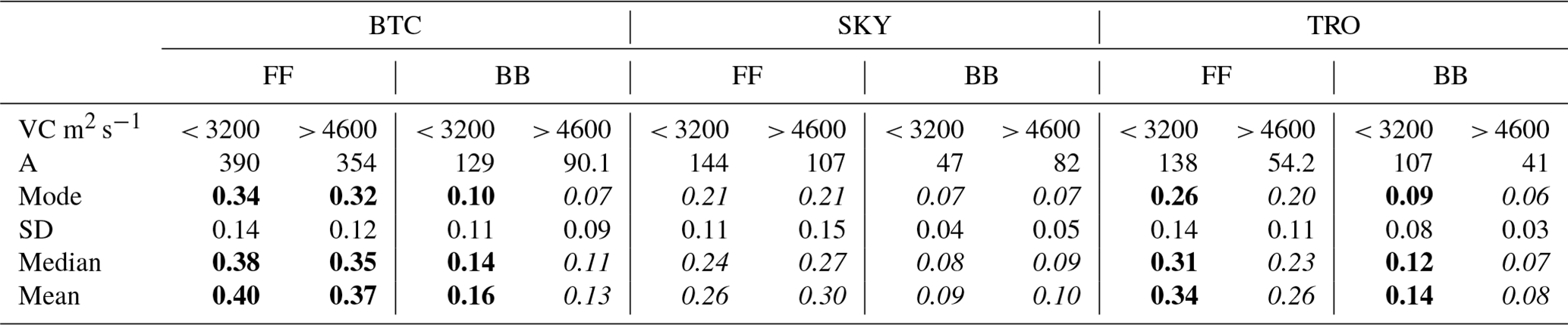
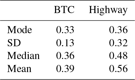
Table 5Fitting parameters of the lognormal distributions of the fossil-fuel-related emission factor (EF, g(kg fuel)−1) at BTC (all data) and the highway. The distributions are normalized to 1. The derived median and mean are also shown.
2.5 Auxiliary measurements
For the validation of the AM-MLR method, a well-defined case is needed with exclusively one type of source (traffic or wood burning). Since this was never the case during winter, we performed additional measurements during summertime next to the E61 highway ring around Ljubljana, where the plumes were expected to originate from pure FF emission sources only. A portable monitoring unit was used for the measurement, including an AE43 Aethalometer (Aerosol d.o.o, Slovenia) and a Vaisala GMP 343 CO2 sensor, as in the winter campaign. The AE43 is a recently released battery-powered portable version of the AE33 Aethalometer with an identical optical chamber, flow system, and operation principle. In addition to its portable setup, the AE43 has a developed firmware and software system that offers improved user experiences with the real-time concentration and pollution-rose plots.
The measurement station was installed on an overpass road above the highway. The overpass makes a connection between two sections of an unpaved road that has negligible traffic (mostly agricultural vehicles), so practically the highway emission dominates the concentrations. Due to the fast fluctuation of the concentration and the short lifetime of the pollution peaks emitted by individual sources, a 1 s measurement time was used.
Since only FF-related sources were measured, the source apportionment and MLR procedures were not needed. The BC and the CO2 concentration increments were well correlated during the peaks, and the slope of the regression was considered the ERFF. Due to the rapid fluctuation of the concentrations, the regression was calculated using a 10 s running time window.
2.6 Uncertainty estimation
The resulting ER values are burdened by uncertainties that originated from several sources, such as (1) the concentration measurements, (2) the BC source apportion, and (3) the MLR calculation. In the following we discuss the different uncertainty sources and estimate the final error of the ER (EF) values.
The measurement is always burdened by a random fluctuation of the readings. As was already mentioned above, the unit-to-unit deviance was 1 % for the BC monitor and 0.4 % for the CO2 sensor. In addition, there is a maximum of 2 % uncertainty of the CO2 measurement and a significantly higher, 25 % systematic error of the BC measurement that comes from the uncertainty in the MAC value and the C factor (Ivančič et al., 2022).
Table 6Emission factors of fossil fuel and biomass burning sources. Comparison of the results of this study with the literature. Results from the present study are shown as mean values and the interquartile range in brackets (q1–q3).
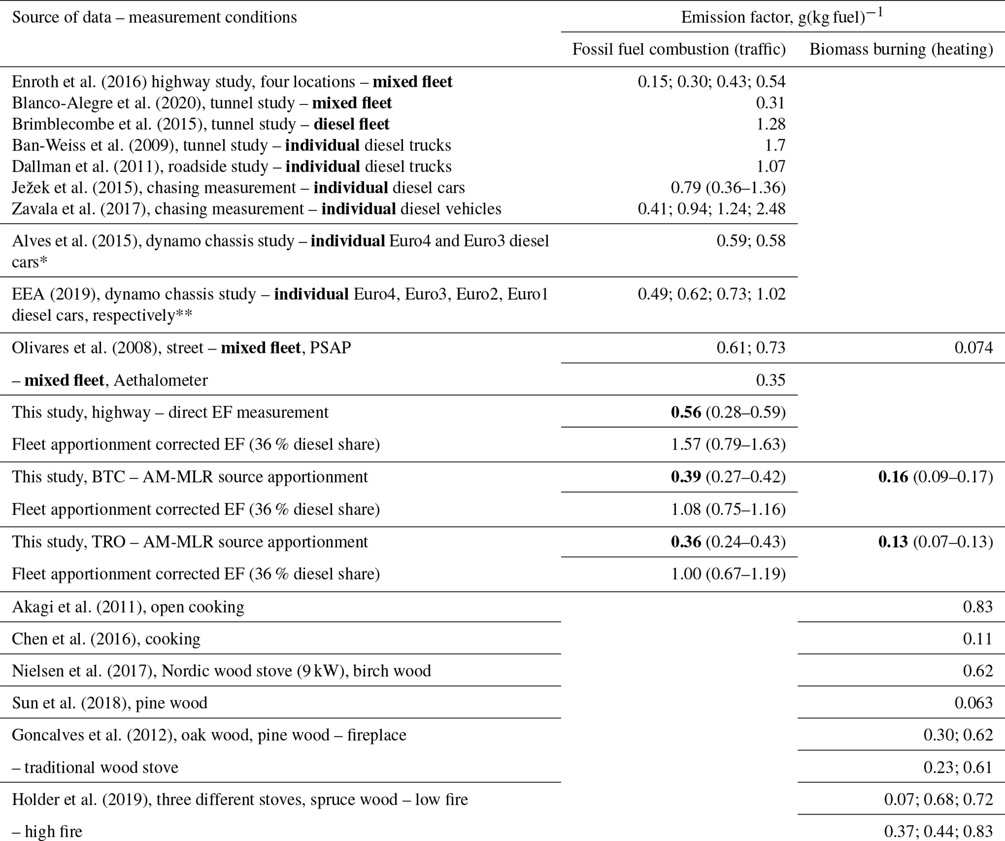
∗ Converted from mg km−1 units using the CO2 EF from the same study. Converted from PM2.5 g km−1 EF using fuel consumption and BC percentage of PM2.5 published by the same study.
The error of the BC source apportionment is caused by the uncertainties in the BB- and FF-related AAEs. Generally, when there is no independent measurement available for correlating the traffic or BB-related BC emissions, this error is estimated as 20 % (Healy et al., 2017). In our case, the source apportionment was combined with a correlation analysis (MLR) that increased the precision of the final values, since only those cases were considered where the source-specific BC–CO2 correlation was high.
The abovementioned random error of the measured data and the uncertainty of the source apportionment result in uncertainties of the BC–CO2 slopes given by the MLR analysis. Besides them, an additional error is generated by the failure of the presumed conditions of the MLR. During the MLR analysis it was assumed that the CO2 background and the ER values are constant during the applied 1 h time window (see Eq. 4). Any significant variation of these parameters during the time window increases the uncertainty of the slopes.
The uncertainties of the slopes given by the MLR analysis performed by the “lm” function of the “stats” package were 6 % for the FF source and 8 % for the BB source on average. This is a combined uncertainty that includes the random error and the source apportionment uncertainty. It is seen that the original 20 % uncertainty was significantly improved by the MLR analysis due to the applied strict threshold of the correlation coefficient (R2=0.9). The systematic 25 % error of the BC measurement increases these uncertainties, so the final uncertainties of the ERs are 31 % for the FF sources and 33 % for the BB sources. The carbon content of the diesel fuel is exactly known, while the wood carbon content also has a ∼7 % uncertainty if the exact type of burnt wood is unknown (see Eq. 1 and the related text). So, the final EFFF uncertainty is the same (31 %), while it is about 40 % for the EFBB.
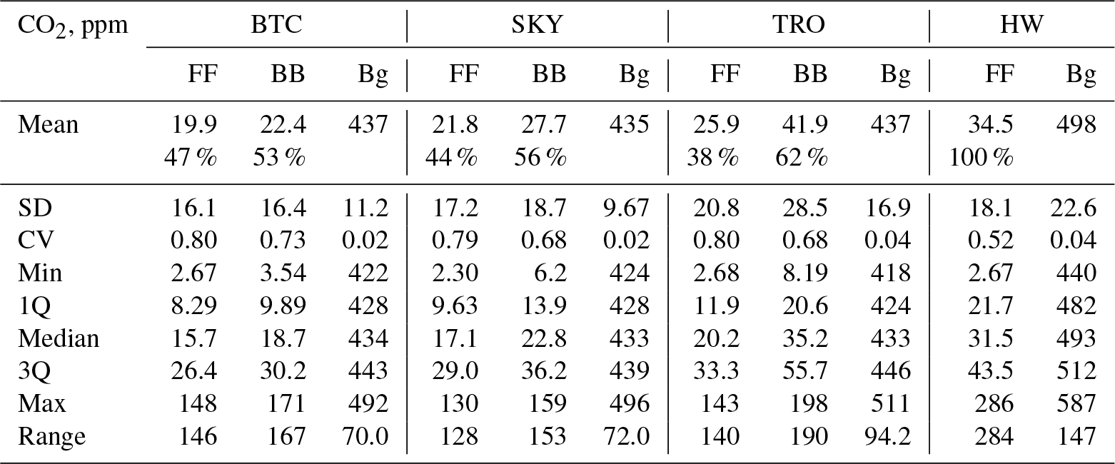
Table 7Source apportionment of the combustion-related CO2 and the background level (Bg) at the three monitoring locations as well as at the highway (FF component only). The mean (with the percental share with respect to the total combustion-related CO2), standard deviation (SD), their ratio (coefficient of variation, “CV”), the three quartiles (1Q, “Median”, 3Q), minimum and maximum values, as well as their difference (“Range”) were calculated from hourly averages for the FF- and BB-related CO2 concentration increments.
3.1 Overview of the measurement results and diurnal cycle of the pollution
The statistical metrics of the hourly measurement averages at the three locations are summarized in Table 2. The BCFF and BCBB fractions are shown separately, as well as the CO2 concentrations, temperature, and relative humidity. The meteorological parameters were measured at the BTC locations only but can be considered generally valid values for the whole city area.
It is seen that the traffic-related BCFF component dominates the BC load at all the locations. The mean BCFF concentrations were 3049, 2200, and 2650 ng m−3 at the BTC, SKY, and TRO locations, respectively, while the corresponding BCBB concentrations were 1595, 1360, and 2180 ng m−3. The biggest difference between the FF- and BB-related components can be observed at the BTC location (64 % vs. 36 % of the total BC), while the smallest one was at TRO (55 % vs. 45 %), indicating a higher influence of wood combustion in the historical center of the city.
The spatial variation of the BC components shows an interesting pattern. Relative to the SKY location, the traffic-related FF component is higher by 38 % at BTC and 36 % at TRO. At the same time, the BB-related BC is higher by 17 % at BTC but 57 % at TRO, indicating that this (TRO) location is a definite hotspot in terms of wood combustion. On the other hand, the influence of traffic emission from the surrounding busy roads is still significant at the TRO measurement site even though it is located in a restricted traffic area.
The BC and CO2 concentrations were highly affected by the atmospheric conditions at all the locations. Figure 3 shows the relationship between the VC and the BC concentration at the BTC and TRO locations. In the background of the figure the frequency distribution of the VC is plotted. The plotted BC values correspond to the average concentrations in the corresponding VC bin. The concentrations follow a decreasing trend with the increasing ventilation, indicating the dilution effect of the atmosphere. A significant concentration drop can be observed between 3200 and 4600 m2 s−1 VC values. It can be interpreted that, in the high concentration interval (BC > 4500 ng m−3, VC < 3200 m2s−1), the local sources dominate the air pollution, while in the low concentration interval (BC < 2500 ng m−3, VC > 4600 m2 s−1) the contribution of transported, diluted pollution is the determinant.
The daily variation of pollution can be followed in the composite day concentration plots shown in Fig. 4. The FF- and BB-related BC concentrations are presented separately. It is seen that a pronounced FF peak can be found in the morning at 08:00 local time at all the locations, representing traffic emissions during the morning rush hours.
By contrast, the BB sources are more active in the afternoon. After 14:00 the BCBB component starts to increase and reaches its daily maximum in the evening. An especially high evening maximum (3500 ng m−3) was found at the BB-influenced TRO location.
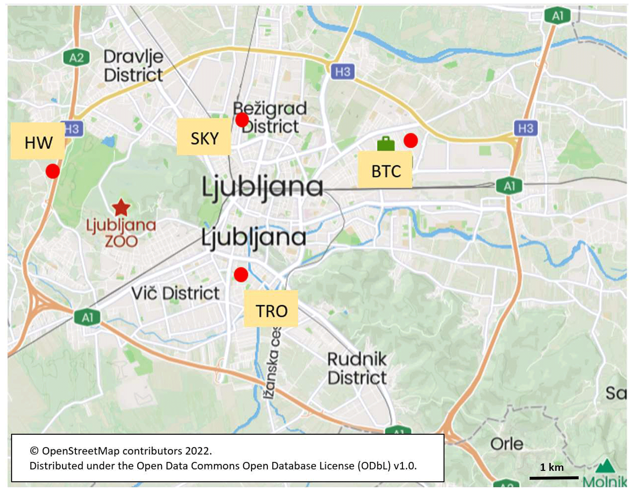
Figure 1Measurement locations on the map of Ljubljana. HW shows the location of the traffic measurement next to the highway.
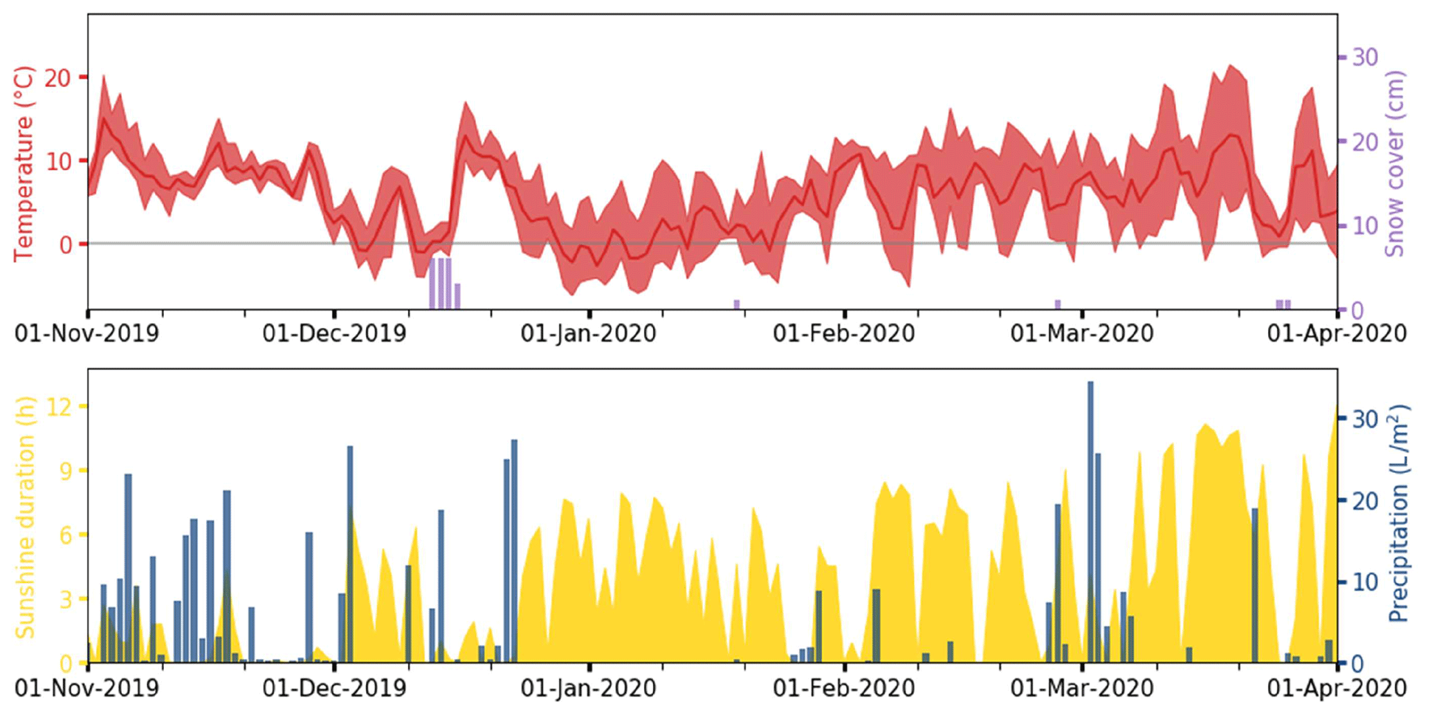
Figure 2Time series of minimal, mean, and maximal daily temperatures, snow cover, daily sunshine duration and daily precipitation accumulation in Ljubljana from November 2019 to March 2020.

Figure 3Frequency distribution of the ventilation coefficient (VC, histogram) and the averaged BC concentrations in the corresponding VC bins at the BTC and TRO locations (scatter plots).
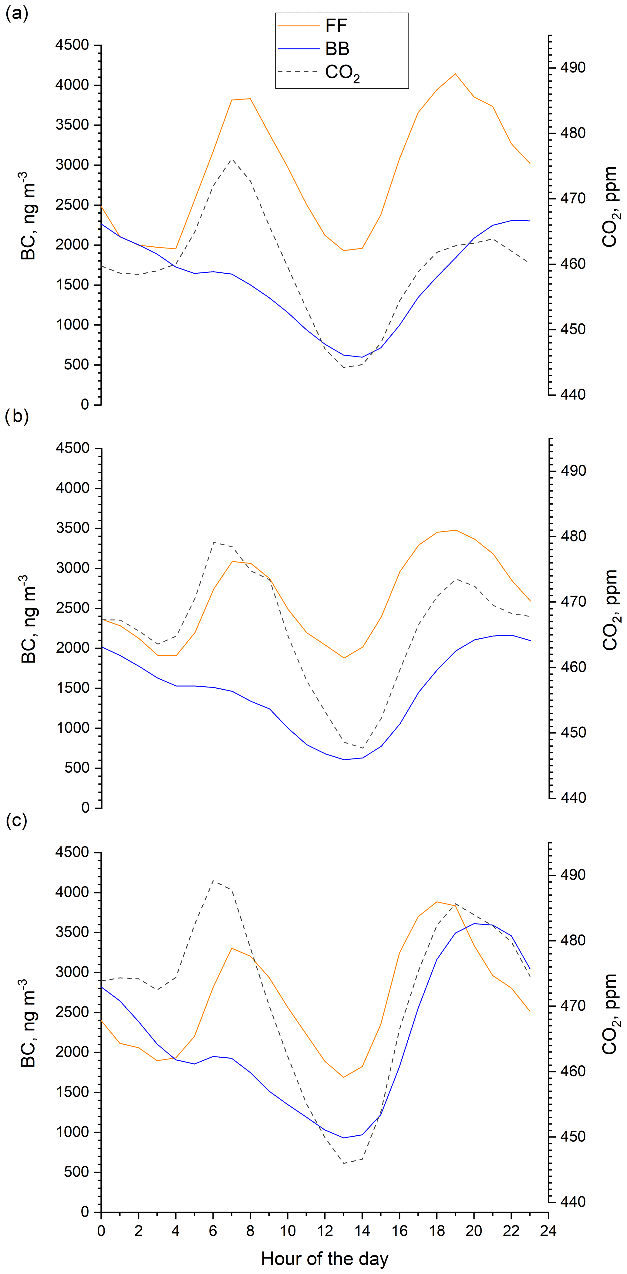
Figure 4Diurnal variation of the FF- and BB-related BC components as well as the CO2 concentration at the (a) BTC, (b) SKY, and (c) TRO monitoring locations. The timescale represents local time.
3.2 2 emission ratios
Using the BC source apportionment results of the Aethalometer model, the MLR analysis provided the CO2 source apportionment and the source-specific emission ratios. The normalized ER distributions are shown in Fig. 5 for the three locations. The distributions are wide and follow a lognormal pattern ranging from 10 to 1000 ng m−3 ppm−1 according to the wide diversity of the sources. Lognormal curves were fitted on the distributions (solid lines in the figures), the parameters of which are summarized in Table 3. The mode and standard deviation that determine a normalized lognormal distribution are presented in the first two rows of the table. Since the median and mean differ from the mode for a lognormal distribution, these derived parameters are also shown in the last two rows of the table.
The wide distribution of ER can be explained by two main reasons. Firstly, the high variety of sources results in a wide range of emission ratios. For example, the BC emission factor of gasoline vehicles varies in the range of 0.001–0.01 g(kg fuel)−1, while that of diesel vehicles falls into the 0.1–10 g(kg fuel)−1 interval (EEA, 2019: 1.A.3.b.). Thus, the measured ER depends on the actual composition of the traffic, moving towards the higher values during the periods when the contribution of diesel sources (e.g., trucks, buses, and goods vehicles) is higher. In contrast, during periods when the traffic is dominated by personal vehicles, the ER decreases due to the higher contribution of gasoline vehicles.
Regarding the BB sources, the contribution of gas heating to the combustion-related CO2 emission must be taken into account. The BC emission of gas heaters is much smaller than that of wood burning (0.6 vs. 74 g GJ−1; EEA, 2019: 1.A.4.b), and thus the contribution of gas burning in the CO2 plume dilutes the BB-related emissions. At the same time, the different burning conditions of wood stows from smoldering to high temperature flaming or the quality of the fuel (wood type, dryness degree) render high divergence of the emission ratios (see low fire–high fire variability in Table 6). More information about the relationship between combustion conditions and BC emissions can be found in the review of Shen et al. (2021).
Additionally, a measurement artifact caused by the high CO2 background level also widens the ER distribution. Typically, the combustion-related CO2 increments were measured in the 8–55 ppm interquartile interval, while the average CO2 background concentration was 437 ppm with a 22 ppm interquartile range (see Table 7). This indicates how quickly a combustion-related CO2 increment can immerse in the fluctuation of the background during the dispersion of the plume. For this reason, sources with high ER (i.e., low CO2 increment) can be detected close to the sources only, and their relative contribution decreases with the increasing distance between the source and the measurement point. Therefore, diluted plumes always provide lower ERs than the direct ones, even if the composition of the sources is similar. Simultaneous measurement of direct and diluted plumes thus results in a wider ER distribution with a lower mode compared to the direct measurement. The same phenomenon leads to lower ER values in well-mixed atmospheres (high VC value) due to the dispersion of the CO2 emission, while atmospheric inversion (low VC value) favors the detection of low CO2 increments, thus resulting in higher ERs.
It is seen in the table that the ERs significantly vary between the locations. Maximal mean ERs were obtained at the BTC location (219 and 161 ng m−3 ppm−1 for FF and BB, respectively), while the minimal mean ERs were found at the SKY location (160 and 100 ng m−3 ppm−1 for FF and BB, respectively).
3.3 Emission factors of biomass burning and fossil fuel combustion
The emission factors were calculated from the ER values for biomass burning and traffic using Eq. (1). However, the dependence of the ER distribution on the pollution dispersion affects the calculated EF distributions as well. Figure 6 shows the EF distributions at the three locations considering two dispersion cases for both components, such as the (1) low-ventilation case (VC < 3200 m2 s−1) and the (2) high-ventilation case (VC > 4600 m2 s−1). The lognormal distribution function was fitted on the data points, and the fitting parameters are summarized in Table 4.
Figure 6a demonstrates that the atmospheric dispersion does not affect the FF emission factor distribution at the BTC site, while the mean BB emission factor is significantly lower in the case of high-ventilation conditions. This means that close FF sources were measured at the BTC site (local traffic), so the ventilation condition does not affect the EF. Regarding the BB component, a mixture of local and distant sources was measured, which later have more contribution with lower EFs during high-ventilation cases that shifted the EF distribution towards the lower EFs.
At the SKY location (Fig. 6b), no difference can be observed in the EF distributions, which indicates that diluted, distant plumes were measured even in low-ventilation cases (negligible contribution of local sources).
At the TRO location (Fig. 6c), both BB and FF emission factors decreased during high-ventilation conditions, but a more pronounced shift can be observed for the FF distribution.
The EFBB mode under high-ventilation conditions at the BTC and TRO locations and the EFFF mode at the TRO location are smaller than that obtained under low-ventilation conditions and match with the corresponding modes at the background (SKY) location (marked by italic numbers; see Table 4). This can be interpreted by the fact that transported plumes dominated the measurements during high-ventilation conditions at all locations and that a direct FF plume was measured at BTC only. It means that EF values under low-ventilation conditions (marked by bold numbers) are less affected by the atmospheric dilution and better estimations of the real emission factors.
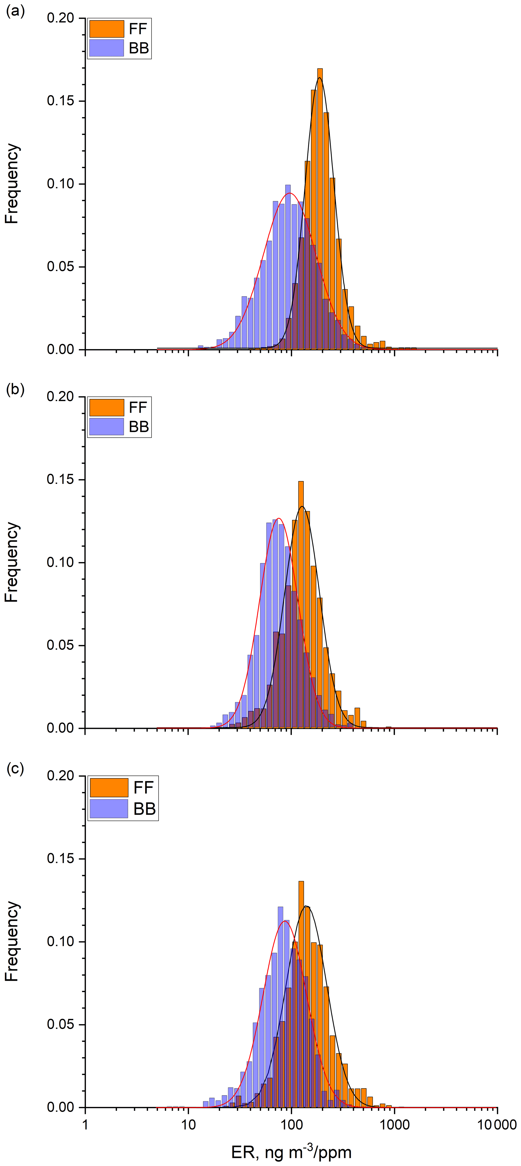
Figure 5FF-related (orange) and BB-related (blue) ERs at (a) BTC, (b) SKY, and (c) TRO locations, respectively. The distributions are normalized to 1. Lognormal distributions (solid lines) were fitted to the results: the parameters are summarized in Table 3.
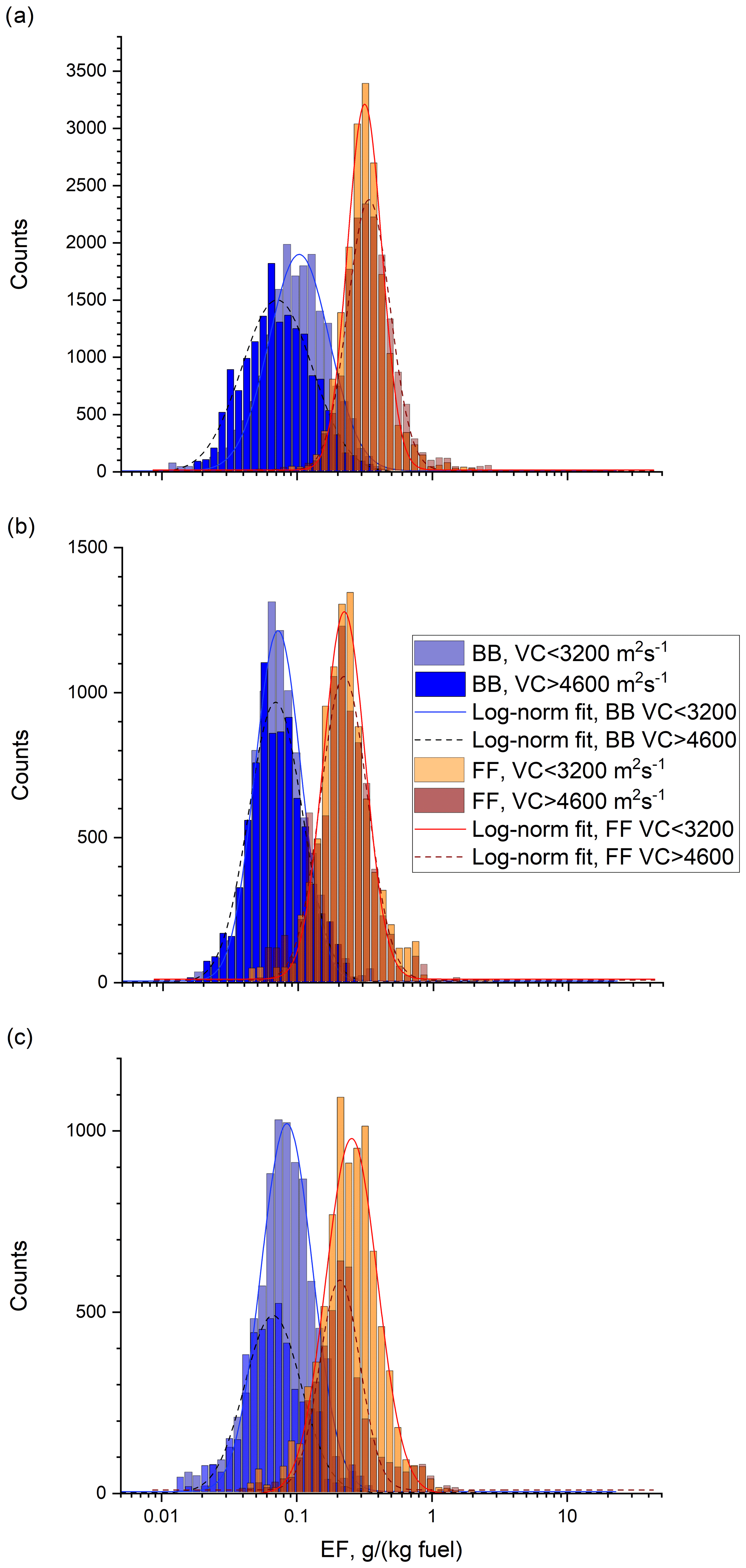
Figure 6FF-related (brown bars) and BB-related (blue bars) emission factors at the (a) BTC, (b) SKY, and (c) TRO locations, respectively. Low (VC < 3200 m2 s−1) and high (VC > 4600 m2 s−1) ventilation cases were plotted separately. Lognormal distributions (solid and dashed lines) were fitted to the results: the parameters are summarized in Table 4.
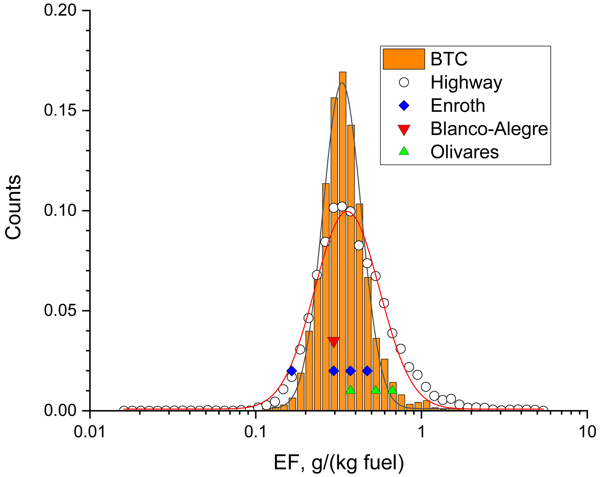
Figure 7Distributions of the emission factors originating from traffic at BTC (all data) and the highway. Lognormal functions were fitted on the points with parameters summarized in Table 5. Colorized scatter symbols refer to the literature data (only X axis concerned). See more details in Table 6.

Figure 8Distribution of the transformed FF EFs referring to the diesel emission at the BTC location (a). Scatter points show average EF data from the literature and the highway measurement (only X axis concerned). (b) Distribution of the BB EFs at the TRO location. Scatter points show average EF data from the literature and the BTC result (only X axis concerned). See more details in Table 6.
In Table 6 we summarize our results together with other data from the relevant literature. Mean values are shown in the table according to the literature data with the interquartile ranges in brackets. The presented data correspond to the low-ventilation case when the EF values were less affected by the atmospheric dilution. Notwithstanding, the comparison with the literature data is still problematic. Our results represent the average case of numerous urban sources involving low BC emitters (or non-smoking sources) that mostly contribute to the CO2 increment (e.g., gas heating, gasoline vehicles). Thus, our results show lower EFs than of individual sources published in the literature. In the following we discuss our results in the context of the literature data considering the abovementioned aspect.
3.3.1 Traffic emission
Since the traffic-related EF does not depend on the ventilation condition at the BTC site, all the measured data were used for EF distribution without the consideration of the VC value. Figure 7 shows the EF distribution at BTC and at the highway that was measured during the summer campaign. The lognormal fits on the measured data are also shown. It is seen that the EF distribution at the highway site is much wider according to the applied short averaging window (10 s) during the correlation analysis that allows us to detect even individual sources. On the other hand, the two distributions covered each other with similar modes (0.33 and 0.36 g(kg fuel)−1 at BTC and the highway, respectively; see Table 5). This good agreement between the AM-MLR method and the pure FF measurement verifies the validity of the AM-MLR method and indicates that the EF values were not distorted by the dilution effect.
In Fig. 7 relevant data from the literature are also shown in scatter plots (see more details in Table 6). Enroth et al. (2016) studied EFs of a mixed fleet in Finland near a highway. Their mean EFs were in the 0.15–0.54 g(kg fuel)−1 range that overlaps with the EF distribution curve at BTC provided by the AM-MLR method.
Blanco-Alegre et al. (2020) measured BC EF in a 1 km-long urban tunnel in Braga, Portugal. Tunnels ensure well-defined conditions for traffic EF measurements with concentrated pollution that mostly originates from vehicle emission. The authors obtained an average EF of 0.31 g(kg fuel)−1 for the fleet of nearly 56 000 vehicles, whose composition is probably similar to the Slovenian fleet (Cooper, 2020). This value is in very good agreement with the result of our AM-MLR method at BTC (0.39 g(kg fuel)−1 average).
Olivares et al. (2008) measured source-specific black carbon concentration in Temuco, Chile, by Aethalometer and particle soot absorption photometer (PSAP). They determined the EF for a mixed fleet by inverse modeling that gave results of 0.35 g(kg fuel)−1 mean EF for Aethalometer and 0.61–0.73 g(kg fuel)−1 EFs for PSAP that fit into our EF distribution.
Assuming that BC emissions of gasoline vehicles are negligible compared to those of diesel engines (as is supported by tailpipe emission measurements – EEA, 2019), all the measured BCFF can be attributed to diesel emission. On the other hand, the diesel-emission-related carbon dioxide can be estimated based on the share of diesel cars in the vehicle fleet, that is, 36 % in Slovenia (National interoperability framework – portal NIO, https://nio.gov.si/nio, last access: January 2023). This means that the diesel-emission-related CO2 is roughly 36 % of the total CO. The emission factor of diesel engines can thus be calculated by dividing the original EF by 0.36.
In Table 6 the transformed EFs are presented for BTC, TRO and highway locations. These numbers refer to the diesel EF only, and they are in good agreement with Brimblecombe et al. (2015), who reported 1.28 g(kg fuel)−1 diesel EF from a tunnel experiment in Hong Kong. The reported EF values from individual diesel cars (Ježek et al., 2015; Alves et al., 2015; Zavala et al., 2017; EEA, 2019) and individual truck emission monitoring (Ban-Weiss et al., 2009; Dallmann et al., 2011) are in good agreement with our transformed EF distribution (Fig. 8a).
3.3.2 Biomass burning
According to the literature data, the biomass burning EF from individual stove emission measurements ranges from 0.063 g(kg fuel)−1 (Sun et al., 2018) to 0.83 g(kg fuel)−1 (Holder et al., 2019; Akagi et al., 2011). The wide dispersion of the literature values indicates the high variety of BB EFs according to the stove type and combustion conditions. Figure 8b demonstrates that most of the literature data fall above our EF distribution measured at the TRO location. The lower EFs we found here can be the consequences of the contribution of gas combustion sources that are common all around the city. Gas burning emits a very small mass of aerosol particles compared to wood combustion, but at the same time, it significantly contributes to the CO2 emissions from domestic heating. Since gas combustion for heating probably has the same time pattern as wood combustion (i.e., concentration increments during the evening and cold weather but drops during the midday and warmer periods), the CO2 increments that correlate with the BCBB component partially originated from gas heating. Our method thus cannot uniquely identify EFs from pure wood combustion but instead refers to the emission factor of the general domestic heating, including non-smoking sources as well. In an ideal case, when the measured sources were exclusively fueled by wood, the heating-related EF would equal the EFBB; otherwise, the higher the contribution of gas heating, the lower the EF.
However, we also note that the real-world EF data published by Olivares et al. (2008) and the stove emission EF for pine wood by Sun et al. (2018) fall on the low end of the EF distribution measured at the TRO location.
3.4 Source apportionment of CO2 emission
Using the source apportionment of BC and the calculated BC ER values, the BB and FF source-related CO2 components can be retrieved. By subtracting the total combustion-related CO2 increment from the measured CO2 level, the non-combustion-related CO2 level can also be determined.
Table 7 summarizes the statistical metrics of the BB and FF source-related CO2 concentrations as well as the background level at the three measurement locations. In addition to the absolute mean values of the BB- and FF-related CO2, their relative contributions to the total combustion-related CO2 concentration are also shown as percentiles.
It is seen that the average background CO2 concentration was the same (∼436 ppm) at all the locations. On the other hand, the source apportionment of the combustion-related CO2 shows significant variation according to the environmental conditions of the locations. At the BTC location the FF-related CO2 component is slightly lower than the BB component (47 vs. 53 %), while at the TRO location, the BB emission dominates the CO2 level (62 %).
Atmospheric concentrations of black carbon and CO2 were monitored in real time at three urban locations in Ljubljana, Slovenia, which had different impacts of traffic and wood burning during the winter heating season. The source-specific BC concentrations from the Aethalometer model were used to apportion the combustion-related CO2 by coupling a multilinear regression method. The analysis presumed two combustion-related sources, namely, domestic heating (biomass burning) and traffic (fossil fuel combustion). The combined AM-MLR method provided consistent and realistic “real-world” emission ratios and emission factors for the three measurement locations. The method can be further generalized for source apportionment of other combustion-related components, and that of EFs can be determined later. Information about the source-specific EFs helps to estimate the pollution emission rates based on the fuel consumption.
The specific conclusions are as follows.
-
The traffic-related BCFF concentration was higher than BCBB at all locations. The smallest difference was found at TRO (wood combustion site), while the largest difference was obtained at BTC (traffic site). In contrast, the heating-related CO2 concentrations were higher at all the locations.
-
The determined ERs follow a wide lognormal distribution according to the variety of the fuels (from the non-smoking gasoline or natural gas to the BC-producing diesel oil and wood) and sources (DPF equipped vs. conventional diesel vehicles; different types and conditions of wood stoves), as well as combustion conditions (high temperature, excess of air vs. low temperature, deficit air conditions). Also, it was shown that the distances of the sources affect the ER, since the relative contributions of high ER sources (means of low relative CO2 emission) are lower for higher distances due to the dilution and fast dispersion of the related CO2 increment.
-
Using the literature data of the carbon content of the fuels (diesel oil vs. wood), the related emission factors (EFs) were determined. The determined mean traffic-related EF (0.36 and 0.39 g(kg fuel)−1 for TRO and BTC, respectively) is in good agreement with published EF values for a mixed traffic fleet. Using the relative ratio of gasoline and diesel fleet for Slovenia, the diesel-emission-related EF could be calculated (1.00 and 1.08 g(kg fuel)−1 for TRO and BTC, respectively), which is in good agreement with diesel emission factors published in the literature.
-
The BB-related mean EF (0.13 and 0.16 g(kg fuel)−1 for TRO and BTC, respectively) is lower than the majority of the relevant literature data reported for individual stoves. The difference might be explained by the CO2 contribution of other, non-smoking combustion sources (i.e., gas heating).
-
The AM-MLR method was validated by direct traffic emission monitoring next to the highway during summertime, when only traffic-related sources were most likely sampled. Thus, the FF-related emission factors could be directly determined without source apportionment. The similarity of the modes of the two distributions (0.33 and 0.36 g(kg fuel)−1 for BTC and HW, respectively) indicates that the AM-MLR method provided reliable results.
Data presented in the paper are available from the authors upon request.
AG and IJ designed the experiments with the supervision and guidance of MR, while BA, MI, and AG carried out the measurements. BA developed the methodology for CO2 source apportionment and EF calculations. AG performed the MLR analysis using the R statistical software package. BA prepared the manuscript with contributions from all the co-authors.
At the time of the research, all the authors of this paper were employed by the manufacturer of the Aethalometer instruments, used to measure black carbon concentration in the study. The funding sponsors had no role in the design of the study, in the collection, analyses, or interpretation of data, in the writing of the manuscript, or in the decision to publish the results.
Publisher’s note: Copernicus Publications remains neutral with regard to jurisdictional claims in published maps and institutional affiliations.
Antony Hansen is thanked for his comments and corrections that helped to finalize the manuscript. Student Klemen Levičnik is thanked for his contribution in the measurement campaigns. Editor Jean-Philippe Putaud and the two anonymous referees are thanked for their valuable comments and recommendations.
This research has been supported by the Ministrstvo za Gospodarski Razvoj in Tehnologijo (grant no. C2130-19-096947) and the Javna Agencija za Raziskovalno Dejavnost Republike Slovenije (grant no. J1-1716 – D).
This paper was edited by Jean-Philippe Putaud and reviewed by two anonymous referees.
Akagi, S. K., Yokelson, R. J., Wiedinmyer, C., Alvarado, M. J., Reid, J. S., Karl, T., Crounse, J. D., and Wennberg, P. O.: Emission factors for open and domestic biomass burning for use in atmospheric models, Atmos. Chem. Phys., 11, 4039–4072, https://doi.org/10.5194/acp-11-4039-2011, 2011.
Alfoldy, B. and Steib, R.: Investigating the Real Air Pollution Exchange at Urban Sites Based on Time Variation of Columnar Content of the Cpmponents, Water Air Soil. Pollut., 220, 9–21, https://doi.org/10.1007/s11270-010-0730-4, 2011.
Alves, C. A., Lopes, D. J., Calvo, A. I., Evtyugina, M., Rocha, S., and Nunes, T.: Emissions from Light-Duty Diesel and Gasoline in-use Vehicles Measured on Chassis Dynamometer Test Cycles, Aerosol Air Qual. Res., 15, 99–116, https://doi.org/10.4209/aaqr.2014.01.0006, 2015.
Ban-Weiss, G. A., Lunden, M. M., Kirchstetter, T. W., and Harley, R. A.: Measurement of black carbon and particle number emission factors from individual heavy-duty trucks, Environ. Sci. Technol., 43, 1419–1424, https://doi.org/10.1021/es8021039, 2009.
Blanco-Alegre, C., Calvoa, A. I., Alves, C., Fialho, P., Nunes, T., Gomes, J., Castro, A., Oduber F., Coz, E., and Fraile, R.: Aethalometer measurements in a road tunnel: A step forward in the characterization of black carbon emissions from traffic, Sci. Total Environ., 703, 135483, https://doi.org/10.1016/j.atmosres.2021.105980, 2020.
Blanco-Alegre, C., Fialho, P., Calvo, A.I., Castro, A., Coz, E., Oduber, F., Prevot, A. S. H., Močnik, G., Alves, C., Giardi, F., Pazzi, G., and Fraile, R.: Contribution of coal combustion to black carbon: Coupling tracers with the aethalometer model, Atmos. Res., 267, 105980, https://doi.org/10.1016/j.atmosres.2021.105980, 2022.
Bond, T. C. and Bergstrom, R. W.: Light Absorption by Carbonaceous Particles: An Investigative Review, Aerosol Sci. Technol., 40, 27–67, https://doi.org/10.1080/02786820500421521, 2006.
Brimblecombe, P., Townsend, T., Lau, C. F., Rakowska, A., Chan, T. L., Mocnik, G., and Ning, Z.: Through-tunnel estimates of vehicle fleet emission factors, Atmos. Environ., 123, 180–189, 2015.
Brown, S. G., Lam-Snyder, J., McCarthy, M. C., Pavlovic, N. R., D'Andrea, S., Hanson, J., Sullivan, A. P., and Hafner, H. R.: Assessment of Ambient Air Toxics and Wood Smoke Pollution among Communities in Sacramento County. Int. J. Environ. Res. Public. Health., 17, 1080, https://doi.org/10.3390/ijerph17031080, 2020.
Chen, Y., Shen, G., Liu, W., Du, W., Su, S., Duan, Y., Lin, N., Zhuo, S., Wang, X., Xing, B., and Tao, S.: Field measurement and estimate of gaseous and particle pollutant emissions from cooking and space heating processes in rural households, northern China, Atmos. Environ., 125, 265–271, 2016.
Chen, J., Li, C., Ristovski, Z., Milic, A., Gu, Y., Islam, M. S., Wang, S., Hao, J., Zhang, H., He, C., Guo, H., Fu, H., Miljevic, B., Morawska, L., Thai, P., Fat LAM, Y., Pereira, G., Ding, A., Huang, X., and Dumka, U. C.: A review of biomass burning: Emissions and impacts on air quality, health and climate in China, Sci. Total Environ., 579, 1000–1034, https://doi.org/10.1016/j.scitotenv.2016.11.025, 2017.
Chiloane, K. E., Beukes, J. P., van Zyl, P. G., Maritz, P., Vakkari, V., Josipovic, M., Venter, A. D., Jaars, K., Tiitta, P., Kulmala, M., Wiedensohler, A., Liousse, C., Mkhatshwa, G. V., Ramandh, A., and Laakso, L.: Spatial, temporal and source contribution assessments of black carbon over the northern interior of South Africa, Atmos. Chem. Phys., 17, 6177–6196, https://doi.org/10.5194/acp-17-6177-2017, 2017.
Cooper, J. (edit): Statistical Report 2020, Fuels Europe, https://www.fuelseurope.eu/wp-content/uploads/SR_FuelsEurope-_2020-1.pdf (last access: January 2023), 2020.
Cuesta-Mosquera, A., Močnik, G., Drinovec, L., Müller, T., Pfeifer, S., Minguillón, M. C., Briel, B., Buckley, P., Dudoitis, V., Fernández-García, J., Fernández-Amado, M., Ferreira De Brito, J., Riffault, V., Flentje, H., Heffernan, E., Kalivitis, N., Kalogridis, A.-C., Keernik, H., Marmureanu, L., Luoma, K., Marinoni, A., Pikridas, M., Schauer, G., Serfozo, N., Servomaa, H., Titos, G., Yus-Díez, J., Zioła, N., and Wiedensohler, A.: Intercomparison and characterization of 23 Aethalometers under laboratory and ambient air conditions: procedures and unit-to-unit variabilities, Atmos. Meas. Tech., 14, 3195–3216, https://doi.org/10.5194/amt-14-3195-2021, 2021.
Dallmann, T. R., Harley, R. A., and Kirchstetter, T. W.: Effects of diesel particle filter retrofits and accelerated fleet turnover on drayage truck emissions at the port of Oakland, Environ. Sci. Technol., 45, 10773–10779, https://doi.org/10.1021/es202609q, 2011.
Deng, J., Guo, H., Zhang, H., Zhu, J., Wang, X., and Fu, P.: Source apportionment of black carbon aerosols from light absorption observation and source-oriented modeling: an implication in a coastal city in China, Atmos. Chem. Phys., 20, 14419–14435, https://doi.org/10.5194/acp-20-14419-2020, 2020.
Drinovec, L., Močnik, G., Zotter, P., Prévôt, A. S. H., Ruckstuhl, C., Coz, E., Rupakheti, M., Sciare, J., Müller, T., Wiedensohler, A., and Hansen, A. D. A.: The ”dual-spot” Aethalometer: an improved measurement of aerosol black carbon with real-time loading compensation, Atmos. Meas. Tech., 8, 1965–1979, https://doi.org/10.5194/amt-8-1965-2015, 2015.
Dumka, U. C., Kaskaoutis, D. G., Tiwari, S., Safai, P. D., Attri, S. D., Soni, V. K., Singh, N., and Mihalopoulos, N.: Assessment of biomass burning and fossil fuel contribution to black carbon concentrations in Delhi during winter, Atmos. Environ., 194, 93–109, https://doi.org/10.1016/j.atmosenv.2018.09.033, 2018.
EEA: EMEP/EEA air pollution emission inventory guidebook. Technical guidance to prepare national emission inventories, EEA Report No 13/2019, ISSN 1977–8449, https://doi.org/10.2800/293657, 2019.
Enroth, J., Saarikoski, S., Niemi, J., Kousa, A., Ježek, I., Močnik, G., Carbone, S., Kuuluvainen, H., Rönkkö, T., Hillamo, R., and Pirjola, L.: Chemical and physical characterization of traffic particles in four different highway environments in the Helsinki metropolitan area, Atmos. Chem. Phys., 16, 5497–5512, https://doi.org/10.5194/acp-16-5497-2016, 2016.
Giechaskiel, B., Bonnel, P., Perujo, A., and Dilara, P.: Solid Particle Number (SPN) Portable Emissions Measurement Systems (PEMS) in the European Legislation: A Review, Int. J. Environ. Res. Pub. Health, 16, 4819, https://doi.org/10.3390/ijerph16234819, 2019.
Giglio, L., Randerson, J. T., and van der Werf, G. R.: Analysis of daily, monthly, and annual burned area using the fourth-generation global fire emissions database (GFED4), J. Geophys. Res.-Biogeosci., 118, 317–328, https://doi.org/10.1002/jgrg.20042, 2013.
Glojek, K., Močnik, G., Alas, H. D. C., Cuesta-Mosquera, A., Drinovec, L., Gregorič, A., Ogrin, M., Weinhold, K., Ježek, I., Müller, T., Rigler, M., Remškar, M., van Pinxteren, D., Herrmann, H., Ristorini, M., Merkel, M., Markelj, M., and Wiedensohler, A.: The impact of temperature inversions on black carbon and particle mass concentrations in a mountainous area, Atmos. Chem. Phys., 22, 5577–5601, https://doi.org/10.5194/acp-22-5577-2022, 2022.
Gonçalves, C., Alves, C., and Pio, C.: Inventory of fine particulate organic compound emissions from residential wood combustion in Portugal, Atmospheric Environment, 50, 297–306, https://doi.org/10.1016/j.atmosenv.2011.12.013, 2012.
Hansen, A. D. A. and Rosen, H.: Individual measurement of the emission factor of aerosol black carbon in automobile plumes, J. Air Waste Manage. Assoc., 40, 1654–1657, 1990.
Healy, R. M., Sofowote, U., Su, Y., Debosz, J., Noble, M., Jeong, C.-H., Wang, J. M., Hilker, N., Evans, G. J., Doerksen, G., Jones, K., and Munoz, A.: Ambient measurements and source apportionment of fossil fuel and biomass burning black carbon in Ontario, Atmos. Environ., 161, 34–47, https://doi.org/10.1016/j.atmosenv.2017.04.034, 2017.
Healy, R. M., Wang, J. M., Sofowote, U., Su, Y., Debosz, J., Noble, M., Munoz, A., Jeong, C-H., Hilker, N., Evans, G. J., and Doerksen G.: Black carbon in the Lower Fraser Valley, British Columbia: Impact of 2017 wildfires on local air quality and aerosol optical properties, Atmos. Environ., 217, 116976, https://doi.org/10.1016/j.atmosenv.2019.116976, 2019.
Helin, A., Niemi, J. V., Virkkula, A., Pirjola, L., Teinila, K., Backman, J., Aurela, M., Saarikoski, S., Ronkko, T., Asmi, E., and Timonen, H.: Characteristics and source apportionment of black carbon in the Helsinki metropolitan area, Finland, Atmos. Environ., 190, 87–98, 2018.
Holder, A. L., Yelverton, T. L. B., Brashear, A. T., and Kariher, P. H.: Black carbon emissions from residential wood combustion appliances, US-EPA report, EPA/600/R-20/039, https://cfpub.epa.gov/si/si_public_record_Report.cfm?dirEntryId=348245&Lab=CEMM (last access: January 2023), May, 2019.
Huss, A., Maas, H., and Hass, H.: Well-to-wheels analysis of future automotive fuels and powertrains in the European context, Tankto-wheels (TTW) report, version 4, EC Joint Research Centre, Luxembourg, https://doi.org/10.2788/40409, 2013.
Ivančič, M., Gregorič, A., Lavrič, G., Alföldy, B., Ježek, I., Hasheminassab, S., Pakbin, P., Ahangar, F., Sowlat, M., Boddeker S., and Rigler, M.: Two-year-long high-time-resolution apportionment of primary and secondary carbonaceous aerosols in the Los Angeles Basin using an advanced total carbon–black carbon (TC-BC(λ)) method, Sci. Total Environ., 848, 157606, https://doi.org/10.1016/j.scitotenv.2022.157606, 2022.
Janssen, N. A. H., Hoek, G., Simic-Lawson, M., Fischer, P., van Bree, L., ten Brink, H., Keuken, M., Atkinson, R. W., Anderson, H. R., Brunekreef, B., and Cassee, F. R.: Black carbon as an additional indicator of the adverse health effects of Airborne particles compared with PM10 and PM2.5, Environ. Health Perspect., 119, 1691–1699. https://doi.org/10.1289/ehp.1003369, 2011.
Ježek, I., Katrašnik, T., Westerdahl, D., and Močnik, G.: Black carbon, particle number concentration and nitrogen oxide emission factors of random in-use vehicles measured with the on-road chasing method, Atmos. Chem. Phys., 15, 11011–11026, https://doi.org/10.5194/acp-15-11011-2015, 2015.
Kalogridis, A.-C., Vratolis, S., Liakakou, E., Gerasopoulos, E., Mihalopoulos, N., and Eleftheriadis, K.: Assessment of wood burning versus fossil fuel contribution to wintertime black carbon and carbon monoxide concentrations in Athens, Greece, Atmos. Chem. Phys., 18, 10219–10236, https://doi.org/10.5194/acp-18-10219-2018, 2018.
Karagulian, F., Belis, C. A., Dora, C. F. C., Prüss-Ustün, A. M., Bonjour, S., Adair-Rohani, H., and Amann, M.: Contributions to cities' ambient particulate matter (PM): A systematic review of local source contributions at global level, Atmos. Environ., 120, 475–483, 2015.
Karanasiou, A., Alastuey, A., Amato, F., Renzi, M., Stafoggia, M., Tobias, A., Reche, C., Forastiere, F., Gumy, S., Mudu, P., and Querol, X.: Short-term health effects from outdoor exposure to biomass burning emissions: A review, Sci. Total Environ., 781, 146739, https://doi.org/10.1016/j.scitotenv.2021.146739, 2021.
Klimont, Z., Kupiainen, K., Heyes, C., Purohit, P., Cofala, J., Rafaj, P., Borken-Kleefeld, J., and Schöpp, W.: Global anthropogenic emissions of particulate matter including black carbon, Atmos. Chem. Phys., 17, 8681–8723, https://doi.org/10.5194/acp-17-8681-2017, 2017.
Liakakou, E., Stavroulas, I., Kaskaoutis, D. G., Grivas, G., Paraskevopoulou, D., Dumka, U. C., Tsagkaraki, M., Bougiatioti, A., Oikonomou, K., Sciare, J., Gerasopoulos, E., and Mihalopoulos, N.: Long-term variability, source apportionment and spectral properties of black carbon at an urban background site in Athens, Greece, Atmos. Environ., 222, 117137, https://doi.org/10.1016/j.atmosenv.2019.117137, 2020.
Mbengue, S., Serfozo, N., Schwarz, J., Zikova, N., Smejkalova, A. H., and Holoubek, I.: Characterization of Equivalent Black Carbon at a Regional Background Site in Central Europe: Variability and Source Apportionment, Environ. Pollut., 260, 113771, https://doi.org/10.1016/j.envpol.2019.113771, 2020.
Milinković, A., Gregorič, A., Džaja Grgičin, V., Vidič, S., Penezić, A., Cvitešić Kušan, A., Bakija Alempijević, S., Kasper-Giebl, A., and Frka, S.: Variability of black carbon aerosol concentrations and sources at a Mediterranean coastal region, Atmos. Pollut. Res., 12, 101221, https://doi.org/10.1016/j.apr.2021.101221, 2021.
Mitchell, E. J. S., Coulson, G., Butt, E. W., Forster, P. M., Jones, J. M., and Williams, A.: Heating with biomass in the United Kingdom: Lessons from New Zealand, Atmos. Environ., 152, 431–454, https://doi.org/10.1016/j.atmosenv.2016.12.042, 2017.
Myhre, G., Samset, B. H., Schulz, M., Balkanski, Y., Bauer, S., Berntsen, T. K., Bian, H., Bellouin, N., Chin, M., Diehl, T., Easter, R. C., Feichter, J., Ghan, S. J., Hauglustaine, D., Iversen, T., Kinne, S., Kirkevåg, A., Lamarque, J.-F., Lin, G., Liu, X., Lund, M. T., Luo, G., Ma, X., van Noije, T., Penner, J. E., Rasch, P. J., Ruiz, A., Seland, Ø., Skeie, R. B., Stier, P., Takemura, T., Tsigaridis, K., Wang, P., Wang, Z., Xu, L., Yu, H., Yu, F., Yoon, J.-H., Zhang, K., Zhang, H., and Zhou, C.: Radiative forcing of the direct aerosol effect from AeroCom Phase II simulations, Atmos. Chem. Phys., 13, 1853–1877, https://doi.org/10.5194/acp-13-1853-2013, 2013.
Naeher, L. P., Brauer, M., Lipsett, M., Zelikoff, J. T., Simpson, C. D., Koenig, J. Q., and Smith, K. R.: Woodsmoke Health Effects: A Review, Inhalation Toxicol., 19, 67–106, 2007.
Nielsen, I. E., Eriksson, A. C., Lindgren, R., Martinsson, J., Nystrom, R., Nordin, E. Z., Sadiktsis, I., Boman, C., Nøjgaard, J. K., and Pagels, J.: Time-resolved analysis of particle emissions from residential biomass combustion – Emissions of refractory black carbon, PAHs and organic tracers, Atmos. Environ., 165, 179–190, 2017.
Ogrizek, M., Gregorič, A., Ivančič, M., Contini, D., Skube, U., Vidović, K., Bele, M., Šala, M., Gunde, M. K., Rigler, M., Menart, E., and Kroflič, A.: Characterization of fresh PM deposits on calcareous stone surfaces: Seasonality, source apportionment and soiling potential, Sci. Total Environ., 856, 159012, https://doi.org/10.1016/j.scitotenv.2022.159012, 2023.
Olivares, G., Ström, J., Johansson, C., and Gidhagen, L.: Estimates of black carbon and size-resolved particle number emission factors from residential wood burning based on ambient monitoring and model simulations, J. Air Waste Manage. Assoc., 58, 838–848, https://doi.org/10.3155/1047-3289.58.6.838, 2008.
Park, G., Kim, K., Park, T., Kang, S., Ban, J., Choi, S., Yu, D. G., Lee, S., Lim, Y., Kim, S., Lee, J., Woo, J. H., and Lee, T.: Characterizing black carbon emissions from gasoline, LPG, and diesel vehicles via transient chassis-dynamometer tests, Appl. Sci., 10, 5856, https://doi.org/10.3390/app10175856, 2020.
Querol, X. (project coordinator): Emission Factors of Biomass Burning, Life-AIRUSE report 9, LIFE11/ENV/ES/584, 2016/12, 1–30, http://airuse.eu/wp-content/uploads/2013/11/R09_AIRUSE-Emission-factors-for-biomass-burning.pdf (last access: January 2023), 2016.
R Core Team: A language and environment for statistical computing, R Foundation for Statistical Computing, Vienna, Austria, https://www.R-project.org/ (last access: January 2023), 2021.
Reddington, C. L., Morgan, W. T., Darbyshire, E., Brito, J., Coe, H., Artaxo, P., Scott, C. E., Marsham, J., and Spracklen, D. V.: Biomass burning aerosol over the Amazon: analysis of aircraft, surface and satellite observations using a global aerosol model, Atmos. Chem. Phys., 19, 9125–9152, https://doi.org/10.5194/acp-19-9125-2019, 2019.
Sánchez-Ccoyllo, O. R., Ynoue, R. Y., Martins, L. D., Astolfo, R., Miranda, R. M., Freitas, E. D., Borges, A. S., Fornaro, A., Freitas, H., Moreira, A., and Andrade, M. F.: Vehicular particulate matter emissions in road tunnels in Sao Paulo, Brazil, Environ. Monitor. Assess., 149, 241–249, https://doi.org/10.1007/s10661-008-0198-5, 2009.
Sandradewi, J., Prevot, A. S. H., Szidat, S., Perron, N., Alfarra, R. M., Lanz, V. A., Weingarten, E., and Baltensperger, U.: Using aerosol light absorption measurements for the quantitative determination of wood burning and traffic emission contributions to particulate matter, Environ. Sci. Technol., 42, 3316–3323, 2008.
Shen, H., Luo, Z., Xiong, R., Liu, X., Zhang, L., Li, Y., Du, W., Chen, Y., Cheng, H., Shen, G., and Tao, S.: A critical review of pollutant emission from fuel combustion in home stoves, Environ. Int., 157, 106841, https://doi.org/10.1016/j.envint.2021.106841, 2021.
Sigsgaard, T., Forsberg, B., Annesi-Maesano, I., Blomberg, A., Bølling, A., Boman, C., Bønløkke, J., Brauer, M., Bruce, N., Héroux, M. E., Hirvonen, M. R., Kelly, F., Künzli, N., Lundbäck, B., Moshammer, H., Noonan, C., Pagels, J., Sallsten, G., Sculier, J. P., and Brunekreef, B.: Health Impacts of Anthropogenic Biomass Burning in the Developed World, Eur. Respir. J., 46, 1577–1588, 2015.
Smirnov, N. S., Korotkov, V. N., and Romanovskaya, A. A.: Black carbon emission from wildfires on forest lands of the Russian Federation 2007–2017, Russ. Meteorol. Hydrol., 40, 435–442, https://doi.org/10.3103/S1068373915070018, 2015.
Sun, J., Zhi, G., Jin, W., Chen, Y., Shen, G., Tian, C., Zhang, Y., Zong, Z., Cheng, M., Zhang, X., Zhang, Y., Liu, C., Lu, J., Wang, H., Xiang, J., Tong, L., and Zhang, X.: Emission factors of organic carbon and elemental carbon for residential coal and biomass fuels in China- A new database for 39 fuel-stove combinations, Atmos. Environ., 190, 241–248, https://doi.org/10.1016/j.atmosenv.2018.07.032, 2018.
Tomlin, A. S.: Air Quality and Climate Impacts of Biomass Use as an Energy Source: A Review, Ener.Fuels, 35, 14213–14240, https://doi.org/10.1021/acs.energyfuels.1c01523, 2021.
Trubetskaya, A., Lin, C., Ovadnevaite, J., Ceburnis, D., O'Dowd, C., Leahy, J. J., Monaghan, R. F. D., Johnson, R., Layden, P., and Smith, W.: Study of Emissions from Domestic Solid-Fuel Stove Combustion in Ireland, Ener. Fuels, 35, 4966–4978, https://doi.org/10.1021/acs.energyfuels.0c04148, 2021.
Val Martin, M., Honrath, R. E., Owen, R. C., Pfister, G., Fialho, P., and Barata F.: Significant enhancements of nitrogen oxides, black carbon, and ozone in the North Atlantic lower free troposphere resulting from North American boreal wildfires, J. Geophys. Res., 111, D23S60, https://doi.org/10.1029/2006JD007530, 2006.
Wang, X., Westerdahl, D., Hu, J., Wu, Y., Yin, H., Pan, X., and Zhang, K. M.: On-road diesel vehicle emission factors for nitrogen oxides and black carbon in two Chinese cities, Atmos. Environ., 46, 45–55, 2012.
Weingartner, E., Saathoff, H., Schnaiter, M., Streit, N., Bitnar, B., and Baltensperger, U.: Absorption of light by soot particles: determination of the absorption coefficient by means of aethalometers, J. Aerosol Sci., 34, 1445–1463, https://doi.org/10.1016/S0021-8502(03)00359-8, 2003.
Yus-Díez, J., Bernardoni, V., Močnik, G., Alastuey, A., Ciniglia, D., Ivančič, M., Querol, X., Perez, N., Reche, C., Rigler, M., Vecchi, R., Valentini, S., and Pandolfi, M.: Determination of the multiple-scattering correction factor and its cross-sensitivity to scattering and wavelength dependence for different AE33 Aethalometer filter tapes: a multi-instrumental approach, Atmos. Meas. Tech., 14, 6335–6355, https://doi.org/10.5194/amt-14-6335-2021, 2021.
Zavala, M., Molina, L. T., Yacovitch, T. I., Fortner, E. C., Roscioli, J. R., Floerchinger, C., Herndon, S. C., Kolb, C. E., Knighton, W. B., Paramo, V. H., Zirath, S., Mejía, J. A., and Jazcilevich, A.: Emission factors of black carbon and co-pollutants from diesel vehicles in Mexico City, Atmos. Chem. Phys., 17, 15293–15305, https://doi.org/10.5194/acp-17-15293-2017, 2017.
Zheng, X., Wu, Y., Jiang, J., Zhang, S., Liu, H., Song, S., Li, Z., Fan, X., Fu, L., and Hao, J.: Characteristics of On-road Diesel Vehicles: Black Carbon Emissions in Chinese Cities Based on Portable Emissions Measurement, Environ. Sci. Technol., 49, 13492–13500, https://doi.org/10.1021/acs.est.5b04129, 2015.