the Creative Commons Attribution 4.0 License.
the Creative Commons Attribution 4.0 License.
 | 16 Mar 2023
Using tunable infrared laser direct absorption spectroscopy for ambient hydrogen chloride detection: HCl-TILDAS
John W. Halfacre
Jordan Stewart
Scott C. Herndon
Joseph R. Roscioli
Christoph Dyroff
Tara I. Yacovitch
Michael Flynn
Stephen J. Andrews
Steven S. Brown
Patrick R. Veres
The largest inorganic, gas-phase reservoir of chlorine atoms in the atmosphere is hydrogen chloride (HCl), but challenges in quantitative sampling of this compound cause difficulties for obtaining high-quality, high-frequency measurements. In this work, tunable infrared laser direct absorption spectroscopy (TILDAS) was demonstrated to be a superior optical method for sensitive, in situ detection of HCl at the 2925.89645 cm−1 absorption line using a 3 µm inter-band cascade laser. The instrument has an effective path length of 204 m, 1 Hz precision of 7–8 pptv, and 3σ limit of detection ranging from 21 to 24 pptv. For longer averaging times, the highest precision obtained was 0.5 pptv with a 3σ limit of detection of 1.6 pptv at 2.4 min. HCl-TILDAS was also shown to have high accuracy when compared with a certified gas cylinder, yielding a linear slope within the expected 5 % tolerance of the reported cylinder concentration (slope = 0.964 ± 0.008). The use of heated inlet lines and active chemical passivation greatly improve the instrument response times to changes in HCl mixing ratios, with minimum 90 % response times ranging from 1.2 to 4.4 s depending on inlet flow rate. However, these response times lengthened at relative humidities >50 %, conditions under which HCl concentration standards were found to elicit a significantly lower response (−5.8 %). The addition of high concentrations of gas-phase nitric acid (>3.0 ppbv) were found to increase HCl signal (<10 %), likely due to acid displacement with HCl or particulate chloride adsorbed to inlet surfaces. The equilibrium model ISORROPIA suggested a potential of particulate chloride partitioning into HCl gas within the heated inlet system if allowed to thermally equilibrate, but field results did not demonstrate a clear relationship between particulate chloride and HCl signal obtained with a denuder installed on the inlet.
- Article
(6034 KB) - Full-text XML
- BibTeX
- EndNote


Growing attention is being given to the role of reactive chlorine in tropospheric oxidation chemistry (Simpson et al., 2015), given its potential impacts on the lifetimes of volatile organic compounds; atomic chlorine reacts with hydrocarbons at rate constants often orders of magnitude greater than those with hydroxyl radical (Burkholder et al., 2015; Atkinson et al., 2006; Jahn et al., 2021), as in Reaction (R1), where R represents an alkane:
Even moderate amounts of such a potent oxidizer could lead to changes in concentrations of O3, NOx, and hydroxyl radicals. However, the high reactivity of atomic chlorine radicals, combined with a lack of effective gas-phase recycling mechanisms, only allows for a small degree of accumulation, with global tropospheric averages estimated to range between 102 and 105 atoms cm−3 (Allan et al., 2001; Pszenny et al., 2007; Wang et al., 2021; Wingenter et al., 1996; Singh et al., 1996). As such, in situ quantitative detection of atomic chlorine radicals remains out of reach. It is instead more practical to study chlorine through relatively more abundant and stable reservoir species, such as hydrogen chloride (e.g., Angelucci et al., 2021), molecular chlorine (e.g., Liao et al., 2014), chlorine monoxide (e.g., Tuckermann et al., 1997), and nitryl chloride (e.g., Osthoff et al., 2008).
Hydrogen chloride (HCl) is of particular interest because it is the most abundant form of inorganic chlorine in the gas phase and acts as both a source and end product of atomic chlorine. Reaction (R1) represents a significant gas-phase HCl formation pathway, but its largest atmospheric source on a global basis is sea salt aerosol via acid displacement (Graedel and Keene, 1995, 1996; Wang et al., 2019; Erickson et al., 1999), in which the presence or uptake of other acids, such as nitric acid (HNO3) or even organic acids (Laskin et al., 2012), shifts the equilibrium of aqueous chloride back toward gas-phase HCl, as in Reaction (R2) (Brimblecombe and Clegg, 1988; Clegg and Brimblecombe, 1986):
Additional contributions to the HCl budget come from volcanic emissions (von Glasow et al., 2009; Graedel and Keene, 1996) and anthropogenic emissions, including coal combustion, biomass burning, industrial processes (e.g., smelting, cement production), and solid-waste incineration (Zhang et al., 2022; Fu et al., 2018; Keene et al., 1999; McCulloch et al., 1999; Ren et al., 2017; Wang et al., 2019). The loss processes for HCl are governed by two major sinks: reaction with hydroxyl radical and deposition. The reaction of HCl with hydroxyl radical in Reaction (R3) directly produces chlorine radicals that can participate in tropospheric oxidation but is relatively slow ( cm3 molecule−1 s−1 at 298 K) (Atkinson et al., 2007):
While deposition of HCl removes a chlorine atom from the gas phase, its eventual uptake into an aqueous solution will produce chloride ions that can be reintroduced into the atmosphere, either by deacidification (as in R2) or via oxidation into other volatile molecular halogens (i.e., Cl2, ICl, BrCl) (Abbatt et al., 2010; Fickert et al., 1999; Frinak and Abbatt, 2006; Knipping et al., 2000; Oum et al., 1998) or nitryl chloride (Behnke and Zetzsch, 1990; Behnke et al., 1997, 1992). Recent field observations and modeling suggest the vast majority of tropospheric HCl can be found within 1 km of the surface, with mixing ratios decreasing with height until reaching the tropopause, where mixing ratios begin increasing again (Wang et al., 2019, 2021; Lee et al., 2018; Haskins et al., 2018). In the lower troposphere, ambient HCl mixing ratios are typically observed between 101 and 103 parts per trillion by volume (pptv), with the highest amounts found in polluted coastal regions (Angelucci et al., 2021; Crisp et al., 2014, and references therein; Tao et al., 2022).
Recent technological advances have enabled the production of suitable instrumentation for online, in situ detection of ambient HCl. Chemical ionization mass spectrometry (CIMS) is one such method and has been previously characterized in laboratory studies by 3σ limits of detection as low as 15 pptv and sensitivities as high as 2–4 counts s−1 pptv−1 (Eger et al., 2019a; Marcy et al., 2004; Roberts et al., 2010). CIMS instruments are also robust enough to deploy on mobile platforms, including aircraft (Marcy et al., 2004; Veres et al., 2008) and ships (Eger et al., 2019b). The primary disadvantages to CIMS exist in the possibility of sampling compounds (e.g., water) that may interfere with the desired ionization chemistry (e.g., Marcy et al., 2004), as well as issues of selectivity arising from non-analytes that create signal interferences at the desired mass-to-charge ratios meant to represent HCl and/or confirm appropriate isotopic ratios and high limits of detection (Eger et al., 2019a; Roberts et al., 2010). Additionally, CIMS instruments can be quite heavy, require low vacuums, have high power consumption, and often require use of large amounts of consumables (e.g., N2 gas).
An alternative, well-understood approach for HCl detection is infrared absorption spectroscopy. Optical methods benefit from analyzing well-defined and spectrally isolated HCl absorption features (Toth et al., 1970; Li et al., 2011), resulting in a virtually absolute and specific measurement technique. Previously published literature for laser-based HCl instrumentation has demonstrated potential efficacy for in situ detection, including cavity-enhanced (Wilkerson et al., 2021; Hagen et al., 2014; Furlani et al., 2021) and multi-pass cells (Harris et al., 1992; Webster et al., 1994; Scott et al., 1999), both of which benefit from path lengths spanning hundreds of meters to kilometers. These instruments have also been tested on mobile platforms, such as ships (Harris et al., 1992), aircraft (Webster et al., 1994), and balloons (Scott et al., 1999; Wilkerson et al., 2021). The development of small, thermoelectrically cooled, inter-band cascade lasers (ICLs) in recent years has increased the portability of these instruments while also allowing the ability to probe the major HCl infrared absorption feature wavelength (∼3.42 µm).
CIMS and optical methods have both proven to be excellent means of gas-phase HCl detection. However, quantitative sampling remains a challenge for all existing measurement techniques. Hydrogen chloride has a large dipole moment and strong hydrophilicity, which makes it susceptible to interactions with polar surface groups or surfaces on which water may be present. This “sticky” behavior results in long instrument response times during HCl concentration changes (e.g., >60 s) under sampling configurations that include sample tubing and particle filters (Furlani et al., 2021). Further, even inert surfaces, such as those made from polytetrafluoroethylene (PTFE) or perfluoroalkoxy (PFA) Teflon, contain sites where HCl or other sticky molecules (e.g., HNO3) may sorb (Roscioli et al., 2016; Neuman et al., 1999; Yokelson et al., 2003); it has also been estimated that PFA Teflon tubing may contain water films between 0.1 and 10 µm thickness at 20 %–50 % relative humidity, which will readily interact with small polar molecules (Liu et al., 2019; Laasonen and Klein, 1997). Several coatings have been reported in the literature to improve sticky-compound transmission, including halocarbon wax applied to glass (Yokelson et al., 2003; Webster et al., 1994), inert silicon coatings applied to stainless steel (Wilkerson et al., 2021), and continual flow of polyfluorinated acid vapor across glass and Teflon (Roscioli et al., 2016).
In this work, we present an optical method for the quantification of HCl: tunable laser infrared direct absorption spectroscopy (TILDAS), combined with a sampling methodology to minimize inlet artifacts. The TILDAS technique has the advantage of being highly sensitive due to its 204 m path length, a fast response time via incorporation of “active passivation”, and being virtually specific for HCl.
2.1 Gases and chemicals
For in-lab experiments, dry air for sample background measurements was generated with an air compressor and dehumidifying system (dew point approximately −60 ∘C, absolute water vapor concentration ∼0.01 %). When testing the effects of water on the sampling configuration in the laboratory, air was manually humidified using a Michell Instruments DG-3 dew point generator. This compressed air system was also used in generating nitrogen (N2) gas with a commercial N2 generator (Infinity NM32L, Peak Scientific Instruments, UK), which was used as carrier gas for active passivation (Sect. 2.3) and permeation sources (Sect. 2.4). During field studies, zero-grade air (270028-L, BOC Limited, UK) and oxygen-free N2 (44-W, BOC Limited, UK) were used for these purposes (Sect. 2.5).
Perfluorobutanesulfonic acid (PFBS, 97 % purity, CAS 375-73-5, Sigma Aldrich, United States) was used to actively chemically passivate inlet surfaces (Sect. 2.3). Concentrated HCl solution (37 % HCl, CAS 7647-01-0, Fisher Scientific, United States) and concentrated nitric acid (HNO3) solution (70 %, CAS 7697-37-2, Fisher Scientific, United States) were used in making permeation source standards (Sect. 2.4). A 5 ppm HCl gas cylinder (diluted in N2, certified as 4.7 ppm ± 5 %, 2760716, BOC Limited, UK) was used as an independent method validation standard (Sect. 2.4).
2.2 HCl-TILDAS
2.2.1 TILDAS design
The HCl-TILDAS instrument was developed at and purchased from Aerodyne Research Inc (ARI). The TILDAS design used herein has been described extensively by McManus et al. (2015, 2011), and we refer the reader to these publications for technical details on the instrument schematic, physical basis of operation, and instrument noise analysis. The underlying principle of the TILDAS technique is infrared absorption spectroscopy. Briefly, light from a 3 µm inter-band cascade laser (operated at 24.03 ∘C) is collected by an objective and is then focused through a flip-in pinhole that is removed during sampling. After this focus, the beam is reimaged into the multi-pass, astigmatic Herriott cell. In addition, a beam splitter enables the laser to travel down a reference path used intermittently to measure and verify the laser tuning rate. The Herriott cell used in this instrument has an effective path length of 204 m and is held to a temperature of 29 ∘C by circulating air past temperature controlled liquid along the sides of the instrument (Oasis Model T-Three). Temperature controlling the interior of the TILDAS mitigates the effects of exterior temperature changes that may cause optical fringe effects in the reported mixing ratios or changes to the mirror and table distances that may affect the path traveled by the laser light reaching the detector.
The instrument software sweeps the laser over the desired spectral window (2925.80 to 2926.75 cm−1), which it can find via strong absorption lines from other spectrally close absorbers, including methane (2926.18 cm−1, 2926.700231 cm−1) and water (2926.456 cm−1, 2926.742 cm−1) (see Fig. A1 for a HITRAN simulation of the transmittance spectrum). These lines are used to fix peak locations via a frequency-locking algorithm in the software. Incident laser radiation (inherent laser linewidth <0.001 cm−1) probes the strong R(R4) H35Cl line (2925.89645 cm−1) of the 1–0 rovibrational absorption band near 3.4 µm (Guelachvili et al., 1981); the line positions for HCl are extremely well known (±0.0002 cm−1), with a corresponding line strength of cm molec.−1 (uncertainties ranging between 1 % and 2 %) (Li et al., 2013). In addition, the laser is coincidentally able to estimate concentrations of methanol (2925.851 cm−1, 2925.998 cm−1), formaldehyde (2925.842 cm−1, 2926.1 cm−1), and nitrogen dioxide (2925.8 cm−1, 2926.128 cm−1). Line strengths for all species are based upon the HITRAN 2016 database (Gordon et al., 2017). Spectral fits are nonlinear least-squares fits of a ∼1 cm−1 spectral window, using a nonlinear least-squares fit that includes a polynomial baseline. Pressure and temperature are included in the fit to account for pressure broadening and rovibrational state populations, respectively. Since the absorbing features in this region are well resolved (FWHM = 0.010 cm−1, which is primarily pressure and Doppler broadened) and included on the spectral fit, spectral interferences for HCl are not expected for typical ambient mixing ratios observed for the above species.
2.2.2 Sampling inlet
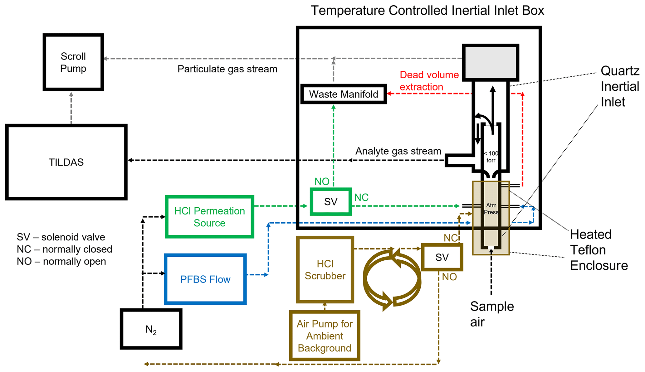
Filtration of particulate matter is required to protect and maintain the efficacy of the multi-pass optics described in the previous section, as well as to reduce the potential of scattering and absorption from particulates within the cell. However, traditional paper filters and filter holders provide surfaces onto which HCl may be removed from the sample stream, both lowering the observed concentration and providing a reservoir of HCl that could be later forced back into the gas phase via an acid displacement mechanism analogous to that which occurs on particulates (i.e., Reaction R2) (Roscioli et al., 2016; Beichert and Finlayson-Pitts, 1996). To obviate this problem, a custom-fabricated quartz virtual impactor (hereafter referred to as “inertial inlet”) was added into the instrument sampling line (Fig. 1). The inertial inlet glass is housed within a temperature-controlled enclosure set to 50 ∘C (Omega CNi32). Sample air that enters the inertial inlet is accelerated through a critical orifice into a low-pressure region (<100 torr). The resulting flow rate through the instrument was determined by the size of this critical orifice in the inertial inlet and cell pressure (set to approximately 40 torr); because different inlets were used for these experiments, experimental flow rates were 2.8, 3.7, or 12.7 L min−1, yielding cell residence times (1/e) of 2.0, 1.5 s, and 0.4 s, respectively. Once in the low-pressure region, particulate separation occurs as follows: large particles (>300 nm diameter) have large forward momentum and maintain their forward flow into a waste flow path (approximately 13 % of the total volumetric flow; flow restriction was dictated by a separate critical orifice installed in the waste flow path). Meanwhile, gas molecules and particles with an approximate diameter <300 nm have less inertia and can make the 180∘ turn necessary to continue along the sample flow path into the TILDAS (approximately 87 % of the total volumetric flow); because the astigmatic Herriott cell used in the TILDAS has a shorter path length and higher light throughput than high-finesse cavity systems, it is not as sensitive to decreased light throughput caused by the accumulation of smaller-diameter particulate matter on cell mirrors. Air flow paths are visualized in Fig. 1. The inertial inlet is connected to the HCl-TILDAS via 3 m of insulated, temperature-controlled (50 ∘C), 9.525 mm PFA Teflon tubing.
2.3 Active passivation
It has been previously shown that adding a small continuous flow of PFBS vapor to sampling lines is effective at increasing transmission of HNO3 through sampling tubing (Roscioli et al., 2016). This technique was used in this work to minimize loss of HCl to surfaces between the inertial inlet and the optical cell. Approximately 5 mL of PFBS was decanted into a bubbler (made from perfluoroalkoxy (PFA) Teflon or Pyrex for laboratory and field studies, respectively) within a chemical fume hood in a laboratory. Given the growing evidence on the deleterious effects of perfluorinated compound accumulation in the environment (e.g., Buck et al., 2011), this bubbler was installed inside a sealed, IP66-rated container to insulate it from potential environmental contamination, as well as to contain any potential spillage in the event of an accident. Compressed N2 gas was passed into the bubbler to flush the headspace (containing PFBS vapor) into the analyte flow path, just after the point of sample air entry into the inertial inlet (Fig. 1). Addition of fresh PFBS vapor into the flow path may quickly release several parts per billion by volume of HCl from unpassivated surfaces and may take several hours to fully condition the system. The temperature and carrier gas flow rate (containing PFBS) were adjusted (between 18 and 22 ∘C and 50 and 100 mL min−1, respectively) until no additional HCl was released to ensure optimal passivation conditions. Release of PFBS vapor from the outlet of the instrument was mitigated by adding a scrubber containing hydroxide salts, glass wool, and activated charcoal to the pump exhaust. When replacement was necessary, the bubbler and any contaminated tubing were washed with absolute ethanol and fully dried before reuse, with rinsings collected and disposed of as hazardous waste.
Passivation efficacy was regularly tested as a function of the timescale of signal change resulting from the addition or removal of HCl standard flow into the inertial inlet (Fig. 1). Timescales were calculated as detailed in Sect. 2.6.2.
2.4 HCl standards for technique validation
Custom HCl permeation sources were created for regular inlet transmission testing using a method modified from Furlani et al. (2021). HCl was pipetted into a 5 cm length of PTFE tubing (3 mm ID, 4 mm OD). Tubing was sealed by heating the ends, one at a time, using a small flame until the tubing became transparent. The end of the tubing was then clamped by pliers and removed from the flame, creating a seal upon cooling. The completed permeation source was then placed in a temperature-controlled aluminum block (set to 35 ∘C). A flow (30 mL min−1) of N2 gas carries the HCl vapor into the instrument flow path (Fig. 1). Additionally, a permeation source for HNO3 was created and utilized in the same manner for the purpose of studying interferences (Sect. 3.3.2).
A cylinder of 5 ppmv (4.7 ± 5 %) HCl (Sect. 2.1) was used to validate the TILDAS response to HCl, although the potential for losses between the cylinder and sample inlet mean that this was not deemed a reliable method for calibration. On opening the cylinder for the first time (or after a period of disuse), multiple days of constant flow (controlled between 1 and 50 mL min−1 by an Alicat MCS-50SCCM) were required to condition the regulator before HCl-TILDAS reflected a stable output. Because TILDAS is an optical method that relies on characteristic, well-described absorption features of molecules, it is considered an absolute detection method and does not require frequent calibrations.
2.5 Field testing
To demonstrate its performance as an in situ, field-ready instrument, the HCl-TILDAS instrument was deployed during the Integrated Research Observation System for Clean Air (OSCA) campaign at the University of Manchester (Manchester, UK, approximately 53.444∘ N, 2.216∘ W), and it sampled HCl between 10 June and 22 July 2021. The OSCA campaign seeks to understand and assess urban air pollution and air quality at various sites across the UK in order to inform and support policy makers in making future decisions and evaluating the impacts of decisions previously made. More information on the campaign and links to relevant studies can be found at the following link: https://gtr.ukri.org/projects?ref=NE%2FT001917%2F1#/tabOverview (last access: 11 November 2022). The measurement site was located at the Manchester Air Quality Super Site on the Firs Environmental Research Station on the University of Manchester campus, and sampled air masses are believed to be heavily influenced by the surrounding urban environment.
The TILDAS instrument and pump for generating background measurements (KNF model N035.1.2AN.18) were installed within an air-conditioned shipping container and held at 25 ∘C. The inertial inlet, HCl permeation source, and active passivation unit were integrated into a separate box (80 cm × 60 cm), installed above the container roof (∼ 3 m a.g.l.) (Fig. 2). Because each of these components are operated at different temperatures (inertial inlet box, permeation source, and active passivation unit held at 50, 35, and 18 ∘C, respectively), the larger box was cooled with a water-cooling fan (controlled to 25 ∘C) to buffer the box interior from changes in the external ambient temperatures and direct solar heating. Temperatures were regularly checked using thermocouples interfaced with an Arduino Uno (Arduino).

Figure 2(a) Field configuration for HCl TILDAS inlet system. (b) Mounted inlet system at Manchester field site.
During the campaign, blank measurements were obtained for 2 min out of every 10 min throughout ambient sampling periods in order to check for drifts in instrument background signal due to optical stability. An effective blank was achieved by passing ambient air through a trap composed of activated charcoal and glass wool. This HCl-scrubbed air was then directed to a Teflon encasing around the inertial inlet, which then overflowed the inlet at approximately 35 L min−1, such that the inlet would only be sampling scrubbed air. To evaluate the inlet for losses and the efficacy of the PFBS, flow from the HCl permeation source was added directly into the inertial inlet on top of the background air overflow for 9 min every 3 h. Note that overblows using zero-air cylinders were found to cause a large increase in HCl signal, followed by a slow decay; it is believed this is due to the sudden disruption in the equilibrium of water molecules adsorbed to instrumentation surfaces. For this reason, permeation source additions under dry air conditions were performed overnight when ambient HCl chemistry mixing ratios were believed to be low. For these experiments, compressed dry air (produced by Jun Air OF302-25MQ2) overflowed the inlet for 1 h, and permeation source HCl was added across three 10 min intervals within this hour.
2.6 Data analysis
Data processing for this work, including background corrections and uncertainty analysis, were conducted primarily using the R statistical software (R Core Team, 2021) in tandem with the RStudio environment (RStudio Team, 2021).
Table 1Summary table comparing the performance of HCl TILDAS to similar previously reported optical methods.
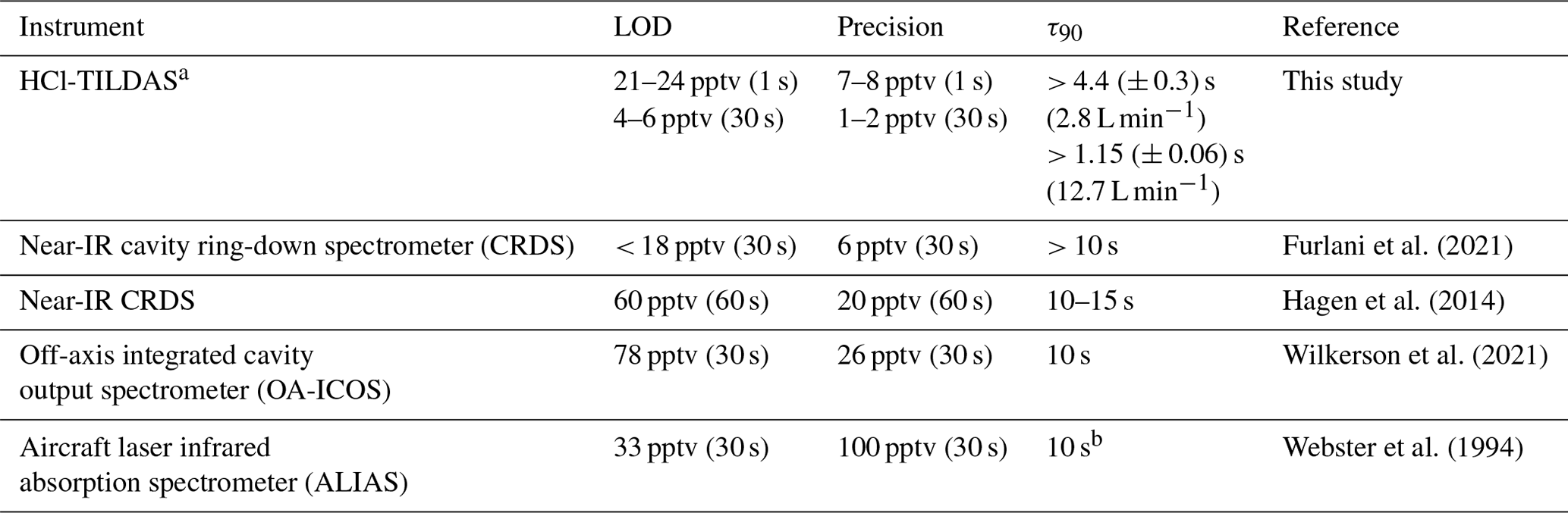
a The lower limit of the figures of merit represent laboratory sampling, while the higher limit represents field sampling. τ90 is reported for dry, laboratory sampling conditions. The lower value represents laboratory analysis, while the higher value represents data from fieldwork (Fig. 9). b Reported for mixing ratio changes > “109 per volume or higher”.
2.6.1 Background correction
As discussed above, background measurements were obtained for 2 min out of every 10 min sampling period. The median of the final 30s of each background period was used as an offset value. Offset values between these points were estimated by linear interpolation and were subsequently subtracted from ambient observations for analysis.
2.6.2 HCl signal response timescales
Timescales of signal decay (τ) after removal of a HCl standard (Sect. 2.4) from the HCl-TILDAS sampling line were calculated as an objective measure of the sampling method performance. Such timescales for sticky gases (including HCl) have been previously determined by fitting data to a bi-exponential model (Roscioli et al., 2016; Zahniser et al., 1995; Ellis et al., 2010; Pollack et al., 2019):
where y represents the HCl mixing ratio, t represents elapsed time, both A1 and A2 are proportionality terms, and both τ1 and τ2 control the shape of the decay curve. Herein, both single-exponential and bi-exponential models were fit to the data to determine the time needed to reach 1/e (τ), 75 % (τ75), and 90 % (τ90) of a starting HCl concentration. The fitting function within R (i.e., “nls”) required initial guesses for the A and τterms, which were based on the starting mixing ratio of HCl and anticipated residence time of air in the absorption cell, respectively; however, the function was not constrained to these values in formulating its output.
2.6.3 HCl partitioning
The thermodynamic equilibrium model ISORROPIA II (Fountoukis and Nenes, 2007), used to investigate K+–Ca2+–Mg2+–NH–Na+–SO–NO–Cl−–H2O aerosol systems, was employed to estimate the potential that particulate chloride (pCl−) may partition to HCl within the heated inlet system. Calculations were performed in “forward mode” when possible, in which the total (gas + aerosol) concentrations of NH3, H2SO4, HCl, HNO3, Na+, Ca2+, K+, and Mg2+ were specified, alongside ambient temperatures and relative humidities. The model then solves a series of equilibrium equations based on these conditions, incorporating water activity equations, activity coefficient calculations, electroneutrality, and mass conservation to determine the gas and aerosol concentrations at thermodynamic equilibrium. The calculations were then repeated for different potential TILDAS sample line testing temperatures (35, 50, and 80 ∘C) to determine changes in gaseous HCl mixing ratios resulting from repartition with aerosols within the sample line. In scenarios where gas-phase concentrations were unknown, the model was initialized in “reverse mode” with averaged aerosol concentrations to predict gas-phase concentrations at equilibrium. In all model calculations, the aerosol was assumed to be in a thermodynamically stable state, in which salts precipitate if saturation is exceeded, owing to the low relative humidities within the heated inlet line.
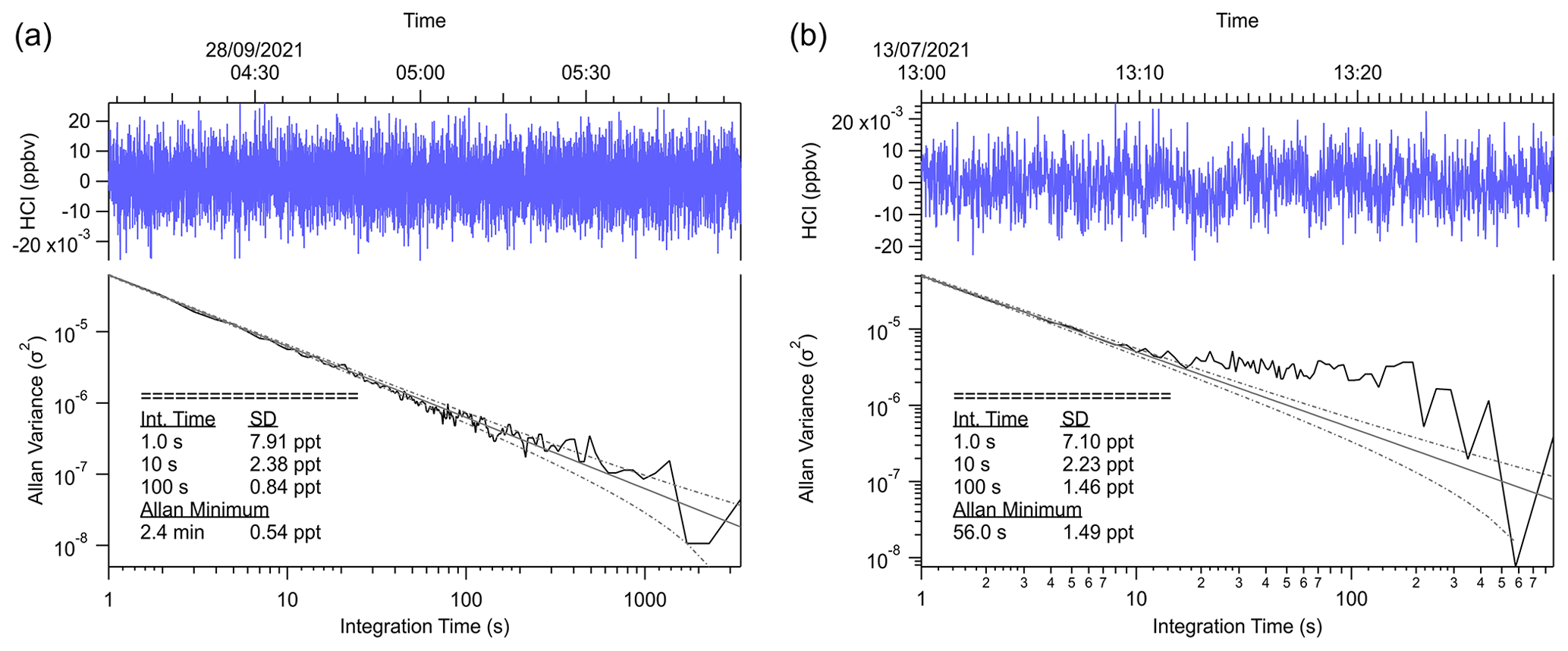
Figure 3Allan variance plot demonstrating the signal variance and limit of detection calculations for varying integration times.
3.1 Instrument performance
The performance metrics of HCl-TILDAS are compared with previously described optical methods in Table 1. Allan–Werle deviations were calculated in the laboratory while overflowing the inlet with dry zero air (Sect. 2.5) (Hagen et al., 2014; Furlani et al., 2021) and in the field with HCl-scrubbed sample air (i.e., without removal of water vapor) (Fig. 3). Using integration times of 30 s and the 3.7 L min−1 inlet, the precision (1–2 pptv at 1σ) and 3σ limit of detection (4–6 pptv) outperform previously reported methods, which range from 6 to 100 pptv precision, and 18–78 pptv limits of detection under 30 s averaging times. HCl-TILDAS has clear advantages for both performance metrics if longer integration times are considered; for dry, laboratory conditions, we achieved a precision of 0.5 pptv and corresponding limit of detection (LOD) of 1.6 pptv at the Allan minimum of 2.4 min, compared with 1.5 pptv precision and 4.4 pptv LOD for field observations at an Allan minimum of 56 s. These values are more than adequate for obtaining high-quality field observations at the expected ambient HCl mixing ratios of 101–103 pptv (Wang et al., 2019). The better performance of the HCl TILDAS is achieved using a long path length (200 m), measuring absorptions in the mid-infrared by probing the fundamental rotational–vibrational absorption band (which has a much larger cross section that in the near IR), and reducing light- and dark-noise levels to equivalent absorbance in 1 s.
A commercial HCl cylinder with a certified concentration (4.7 ppm ± 5 %) was used as an objective standard for in-lab validation. Mixing ratios were varied by adjusting the flow rate of the cylinder output, which was then directly injected into an inertial inlet sidearm (Fig. 1) for direct injection into the passivated inertial inlet. Standard HCl was then diluted into the dry, HCl-free compressed air being sampled by TILDAS. The slope obtained (0.964) was found to lie within the expected 5 % uncertainty reported by the manufacturer, reflecting high accuracy for TILDAS observations (Fig. 4). However, additional sources of error causing deviation from unity must be considered. For example, multiple days of HCl cylinder flow are required for the output mixing ratio to stabilize at its maximum concentration (as observed by TILDAS) after opening the cylinder; this behavior is presumably caused by uptake of HCl onto the metal cylinder regulator and Teflon tubing lines until they are fully conditioned, causing the observed signal to register lower than expected. Changes to HCl cylinder flow additionally require similar conditioning time to re-establish signal stability, likely caused by changes to the HCl gas–surface equilibrium. Thus, although the cylinder was filled with a certified concentration, we were unable to independently confirm that this matched what was ultimately delivered to the TILDAS, with an observed concentration lower than the certified being most likely due to loss onto surfaces. We therefore use this comparison as a validation of this method (not a calibration) using the spectroscopy described above.
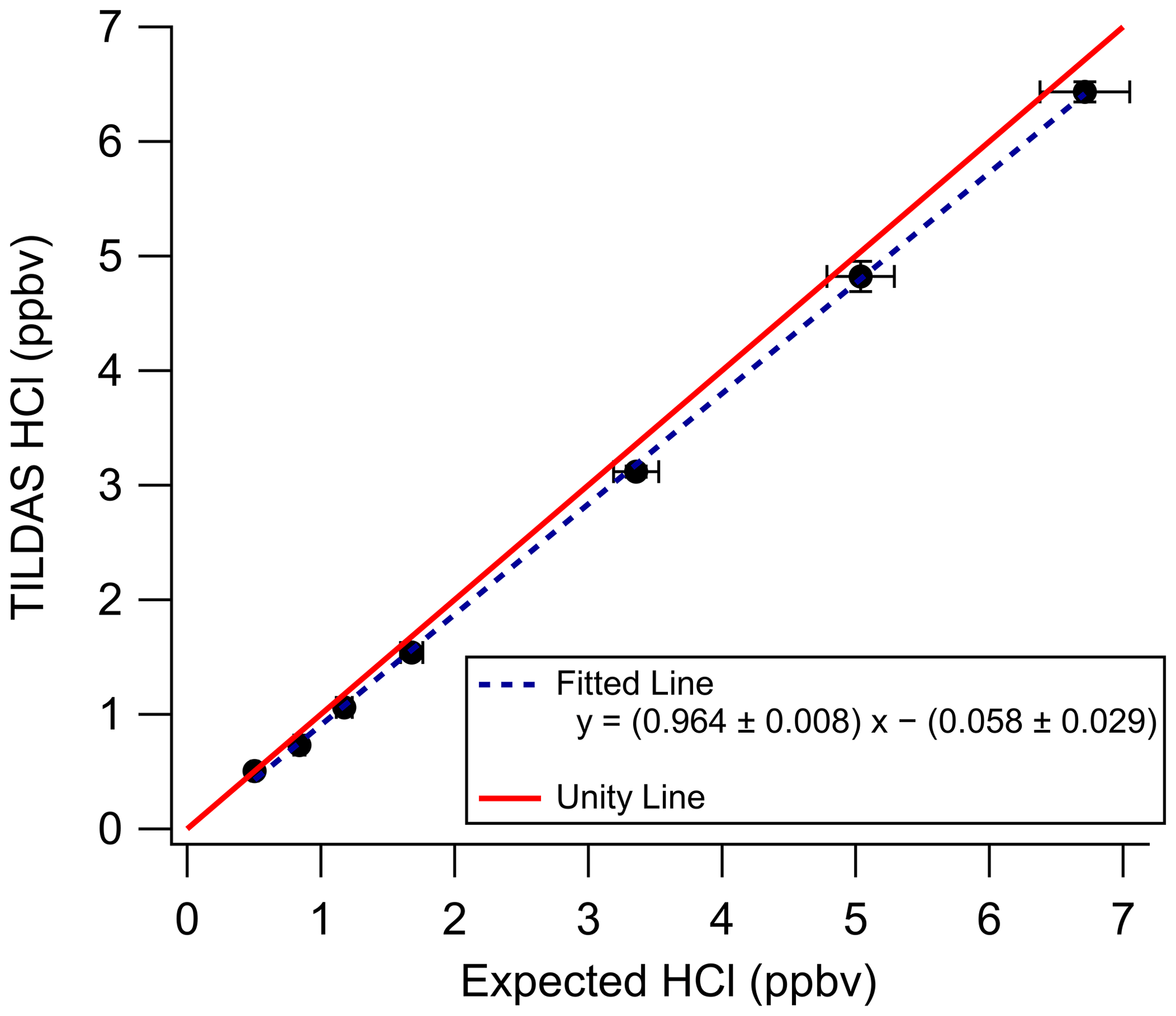
Figure 4In-lab validation of HCl-TILDAS by a commercial HCl standard. Principal axis error bars represent the 5 % uncertainty associated with the HCl standard (as reported by the manufacturer), while the vertical axis error bars represent 1 standard deviation of HCl-TILDAS observations for each validation point. Note the regression line is used here only for the purposes of technique validation and is not used for calibrating data.
3.2 Evaluation of sampling method
Multiple variables were found to affect HCl transmission through the instrument flow path (Fig. 1), including the presence or absence of active passivation (i.e., whether PFBS is flowing through the sample line; Sect. 3.2.1) and the presence of water vapor (Sect. 3.2.2). The timescales of signal change after removal of an HCl source were used to objectively compare the relative effects of each variable. They further allow for direct comparison of the performance of this HCl sampling method with those previously published (Table 1). Note that these timescales reflect how quickly HCl mixing ratios change within the 1.8 L measurement cell and do not include the time required for the sample gas to reach the cell (i.e., time zero is when a change in signal is first observed, not from when an addition valve was triggered).
3.2.1 Active passivation
To test the effectiveness of active passivation, HCl permeation source flow was added into the TILDAS sample line for 10 min of subsequent 30 min periods using the inertial inlet with the lowest flow rate (2.8 L min−1), as the effects of HCl–wall interactions would be the most exaggerated. Experiments were repeated both with and without the coinciding flow of PFBS (Fig. 5), and the TILDAS inlet was overflowed with dry, compressed air (Sect. 2.1), such that a baseline signal was observed in the absence of permeation source addition. We note the permeation source concentration for these experiments was 4.1 ± 0.3 ppbv; the average standard deviation during the last 5 min of permeation source additions was calculated to be 8 ± 2 pptv, while the average standard deviation of the last 5 min of background periods was calculated as 7 ±1 pptv, demonstrating nearly identical precision values while sampling blanks or fixed HCl concentrations. As seen in Fig. 5a, employing active passivation yields sharp, square wave-like behavior on both addition and removal of the HCl permeation source flow. From the fits of a single-exponential model, τe averaged 1.9 ± 0.2 s (N=21) after HCl permeation source removal (Figs. 5b, A2), which compares well with the predicted absorption cell residence time (1/e) of 2.0 s. Though a bi-exponential model was also fit to these data (and achieved comparable τe, τ75, and τ90 values, Table A1), the convergence tolerance of the nonlinear least-squares solving algorithm (Sect. 2.6.2) had to be loosened by 6 orders of magnitude (from a default value of to 2×101) to achieve convergence, suggesting these results are not meaningful. Indeed, the errors for the predicted variables often greatly exceeded the magnitude of the associated variables themselves, suggesting that a bi-exponential model is not appropriate for these actively passivated data.
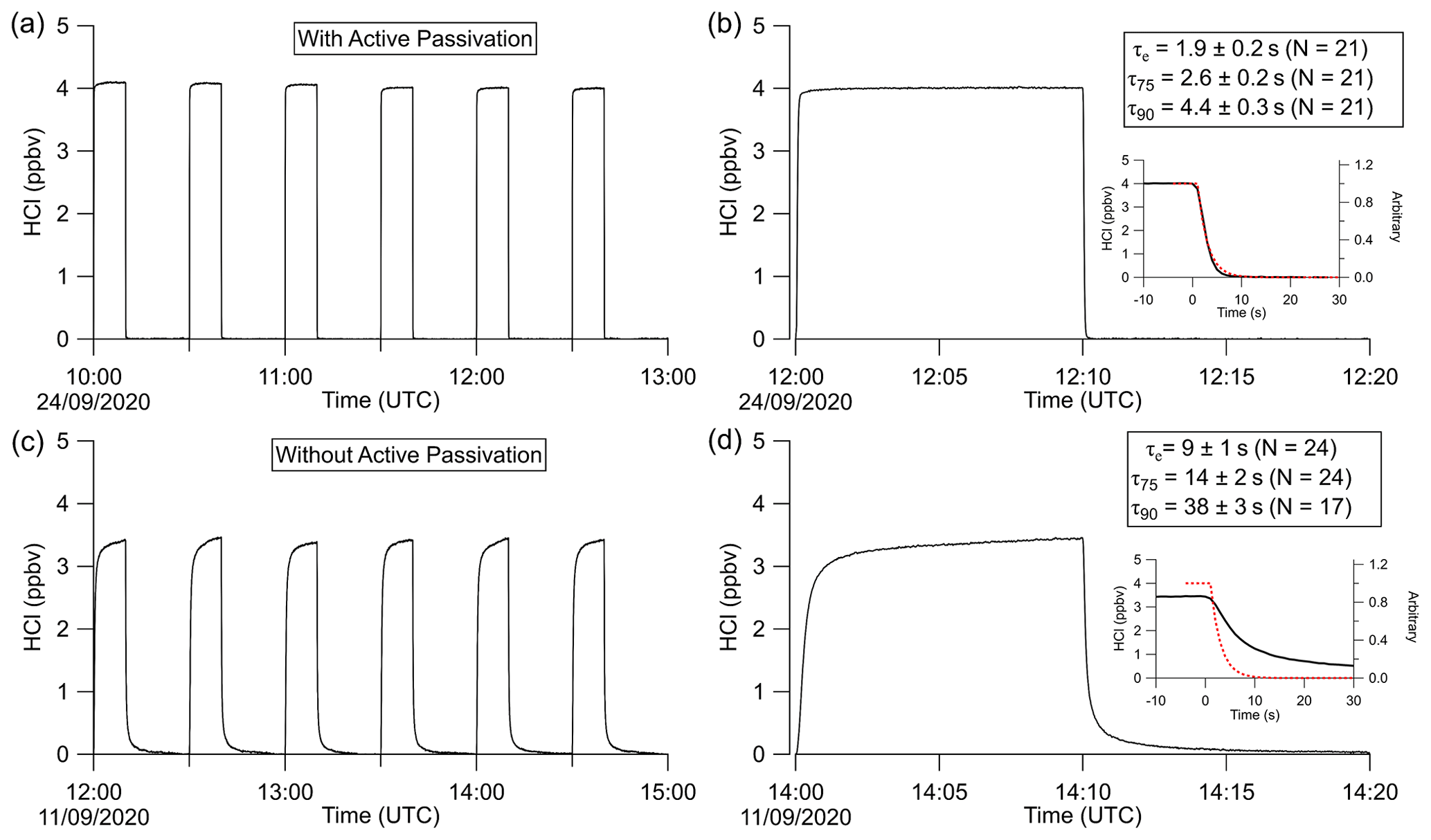
Figure 5Excerpted time series of HCl permeation source additions with (a, b) and without (c, d) use of active passivation. (a) TILDAS response to HCl permeation source addition to the sample line for 10 min every 30 min. (b) Example case from panel (a) demonstrating the profile of the decay timescales. Reported τ′s values represent the mean and standard deviation of the entirety of these experiments. Inset shows a close-up of the actual decay compared with the dashed red line, representing the theoretical decay profile of a non-sticky compound modeled on the residence time of air in the absorption cell. Panels (c) and (d) are analogous to (a) and (b) but without use of active passivation.
Without active passivation, the signal profiles of the HCl additions have comparatively slower rises and do not reach the average HCl maximum mixing ratios of 4.03 ± 0.06 ppbv within 10 min intervals (Figs. 5a, b, A3). In these cases, bi-exponential models were fit without having to adjust the default convergence tolerance, and the results were found to have smaller term and residual errors when compared to the analogous single-exponential model (see Table A2); τe for the signal decays was calculated as 9 ± 1 s (N=24), approximately 4.5 times greater than the residence time through the measurement cell (Fig. 5c, d).
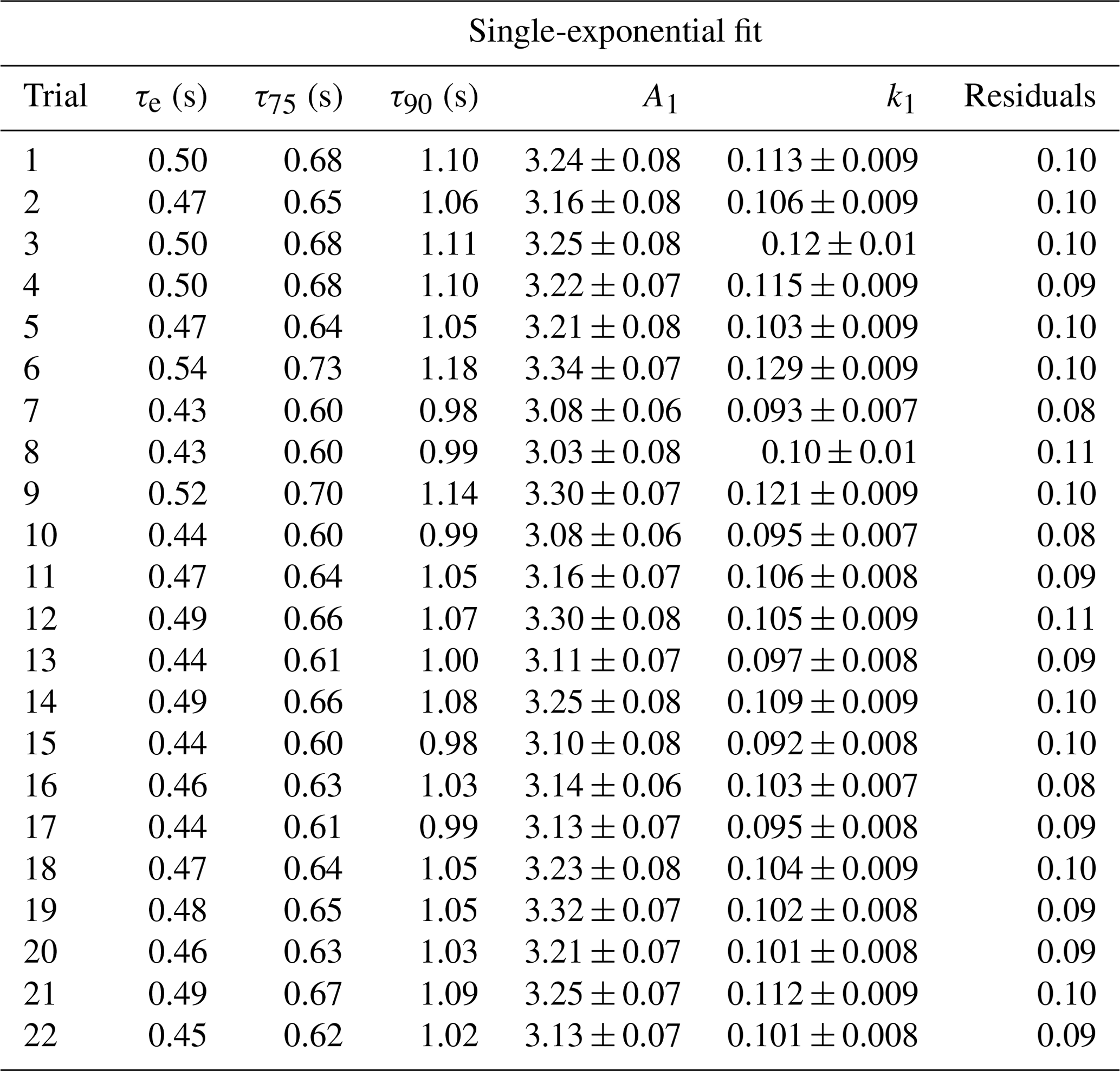
The reported timescales in this work can be further improved by increasing the flow rate of the inlet. Using the 12.7 L min−1 inertial inlet, τe averaged 0.49 ± 0.03 s (N=21), comparing very well to the theoretical cell residence time (1/e) of 0.45 s for this flow rate (Figs. 6, A4, Table A3). τ90 was similarly improved, averaging 1.15 ± 0.06 s. The higher flow rate clearly demonstrates that wall interactions are reduced; as demonstrated by Fig. 6, the decay rate mimics that of methane, which is a non-sticky compound also measured by the HCl-TILDAS. As the current configuration includes 3 m of heated tubing between the inertial inlet and the HCl-TILDAS itself, it is likely this response could be further improved by shortening this line.
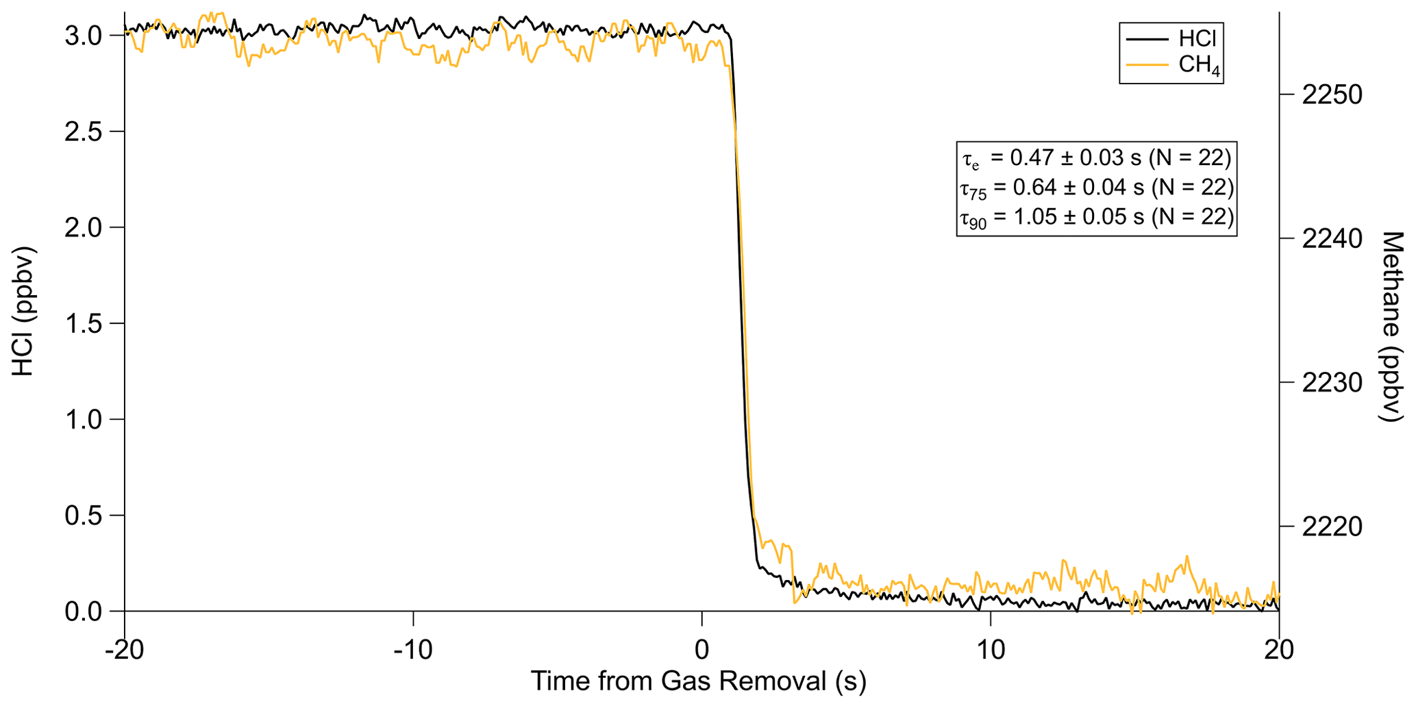
Figure 6Comparison of HCl decay with methane at an inlet flow rate of 12.7 L min−1. Note that the methane signal represents the change in concentration from sampling a zero-air cylinder (∼2260 ppbv) to sampling ambient air (∼2215 ppbv).
The τ90 achieved utilizing active passivation in this study is the shortest reported instrument response time for changes in HCl mixing ratios to date (Table 1) and demonstrates that the use of PFBS is effective for reducing HCl–surface interactions. Previous studies have suggested that a bi-exponential model (Eq. 1) may better physically represent sticky gas flow through an instrument (Furlani et al., 2021; Zahniser et al., 1995; Ellis et al., 2010; Pollack et al., 2019); in this approach, τ1 may represent the air residence time within the instrument, while τ2 will represent the factor(s) that cause the analyte to lag through the instrument (e.g., surface interactions). Our results were not inconsistent with this postulation since the unpassivated cases were well represented by the bi-exponential model (i.e., significant τ1 and τ2 equation terms within Eq. 1), while passivated cases were better represented by the single-exponential model (i.e., dominant τ1 but negligible τ2). However, the results do not directly support this either; for unpassivated cases, the predicted τ1 averaged 6.2 ± 0.7 (greater than 3 times the cell residence time for the inertial inlet used), and 69 ± 10 for τ2 (Table A2). Further reconciliation of the physical basis behind the bi-exponential model is outside the scope of this work, and no attempt is made to ascribe further physical meaning to the derived coefficients.
3.2.2 Humidity
The experiments in the previous sections were conducted using dried compressed air. As dry air is not representative of ambient sampling conditions, timescale experiments were also performed with humidified sample air under passivated conditions. The results in Fig. 7a demonstrate a clear increase in τ values with increasing relative humidity, affecting τ90 most prominently.
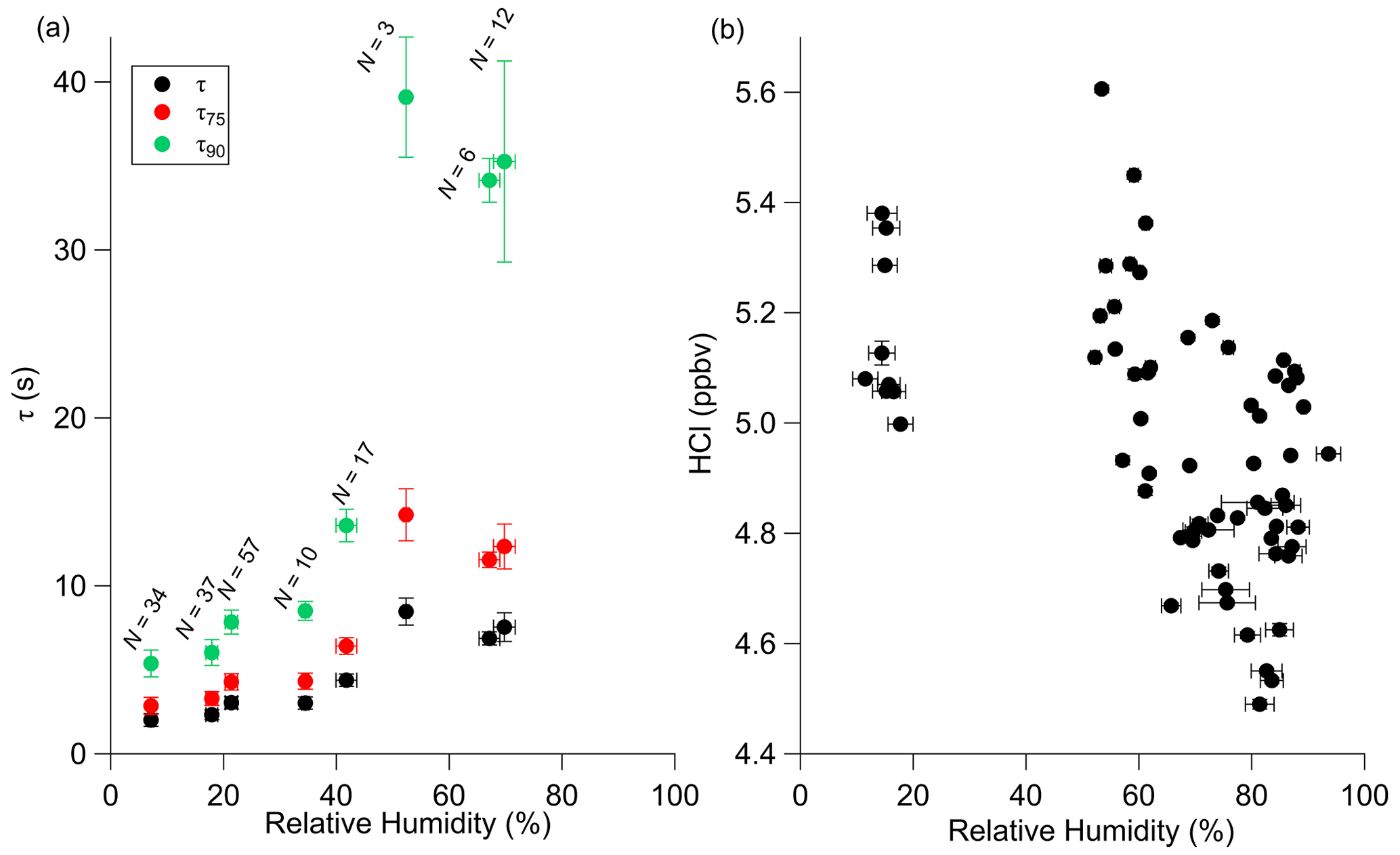
Figure 7Effects of changes in relative humidity on τ during laboratory experiments (a) and HCl standard mixing ratios in the field(b). Relative humidity values are based on the TILDAS-observed water mixing ratio observed during the HCl decay period (a) or HCl standard addition (b) and concurrent temperature reading. Error bars for both axes represent 1 standard deviation.
While Roscioli et al. (2016) note that the general effectiveness of active passivation on HNO3 instrument response times appeared to be independent of humidity levels between 0 % and 70 %, the results of this experiment do not display this same behavior above approximately 40 % relative humidity. Notably, the inlet flow rate used for these experiments is less than 4 times that used in that study (i.e., 2.8 vs. 14 L min−1), which would increase analyte–surface interactions. However, these values do represent an improvement from the HCl sampling method reported by Furlani et al. (2021), in which τ90 was reported as 239 s at 33 % relative humidity. Similarly, Fig. 7b demonstrates that field additions of a HCl permeation source (utilizing the 3.7 L min−1 inertial inlet) elicited lower mixing ratios at relative humidities between 60 % and 93 % (mean of 4.9 ± 0.2 ppbv), contrasting with additions under dry air conditions (i.e., relative humidity < 20 %; mean of 5.2 ± 0.1 ppbv). This finding suggests that a permanent or semi-permanent physical loss of HCl is occurring within the sampling inlet at higher humidities, resulting in an average −5.8 % bias. Both PFA tubing and silica surfaces have been previously reported to adsorb several monolayers worth of water at room temperature in humid air (Saliba et al., 2001; Sumner et al., 2004), which would be expected to bind and solvate HCl. As both the inertial inlet and sample line were heated to 50 ∘C, it is anticipated that this effect would be minimized but not eliminated by discouraging water from attaching to surfaces. However, increasing the sampling temperatures may further improve both the instrument response timescale and reduce this loss effect; warmer temperatures may also increase the likelihood of HCl degassing from coarse-mode particles within the inertial inlet before their removal or from fine-mode particles that may travel throughout the entire sample path (Brimblecombe and Clegg, 1988). Further discussion of the effects of particulate chloride and uncertainty estimation can be found in Sect. 3.3.1.
3.3 Potential interferences
As discussed above, spectral interferences are not believed to play a major role in the detected HCl concentrations. However, two potential sources of undesired HCl may exist if sample gas contains a significant amount of particulate chloride (pCl−) or other strong gaseous acids (e.g., HNO3), discussed in more detail below.
3.3.1 Effects of particulate chloride
It is well established that HCl and particulate chloride (pCl−) exist together in dynamic equilibrium (Fountoukis and Nenes, 2007; Clegg and Brimblecombe, 1986; Brimblecombe and Clegg, 1988; Beichert and Finlayson-Pitts, 1996). The use of heated sample inlet lines (50 ∘C in this study) may volatilize HCl from pCl− if sufficient heating occurs before particles are removed via impaction, yielding measurements with positive systematic error. As discussed in Sect. 2.6.3, the thermodynamic equilibrium model ISORROPIA II was used to theoretically assess the impact of pCl− volatilization within the heated TILDAS sample inlet on measured HCl mixing ratios based on three potential operating temperatures (35, 50, and 80 ∘C). To simulate conditions of an inland, urban environment, averaged aerosol concentrations from London, UK, were used to initiate the model (Bandy et al., 2012; Lee and Young, 2012; Crilley et al., 2017; Lee et al., 2021). It was estimated for the conditions of these measurements that HCl repartitioning from pCl− would result in an increase in the HCl mixing ratio by 1 ppqv at both 35 and 50 ∘C, while dramatically increasing to 200 pptv at 80 ∘C. Such increases in HCl are expected to derive from the loss of the liquid aerosol phase following the reduction in humidity experienced in the elevated temperatures of the sample inlet, and the evaporation of NH4Cl. However, Huffman et al. (2009) reported the evaporation of only approximately 10 %–15 % NH4Cl aerosol through a thermodenuder held at 50 % (12 s residence time). Based on an inertial inlet flow rate of 2.8 L min−1 and a corresponding residence time of 150 ms before particulate removal via impaction, it is unlikely volatilization will significantly affect these measurements. Further in situ testing was performed during the OSCA field study (discussed further in Sect. 3.4).
3.3.2 Effects of nitric acid
The use of PFBS appears to lessen the effects of HCl surface adsorption and improve the instrument response time to changes in HCl concentrations (Figs. 5, 6). If, though, PFBS does not completely prevent HCl sorbing to walls, the sampling of acids stronger than HCl (e.g., HNO3, H2SO4) may perturb the existing passivation equilibrium on instrument surfaces. In order to test this, a HNO3 permeation source was fabricated (Sect. 2.4) and allowed to flow into the TILDAS inlet (Fig. 8). The HNO3 permeation source output was estimated by converting it to NO using a molybdenum catalyst and was subsequently quantified with a commercial NOx analyzer (Teledyne T200). In a test experiment, the addition of 3.0 ppbv of HNO3 to the inertial inlet caused a maximum increase of 0.25 ppbv to the HCl signal (Fig. 8). Continued addition of HNO3 eventually causes the signal to plateau at a higher background, ∼0.08 ppbv above the original background. This experiment was designed as a worst-case scenario, as the TILDAS had been periodically sampling a high-concentration HCl permeation source prior to the HNO3 addition (as would be the case during field operation). This results in more HCl exposure to inlet surfaces than otherwise would be present from purely ambient sampling conditions.
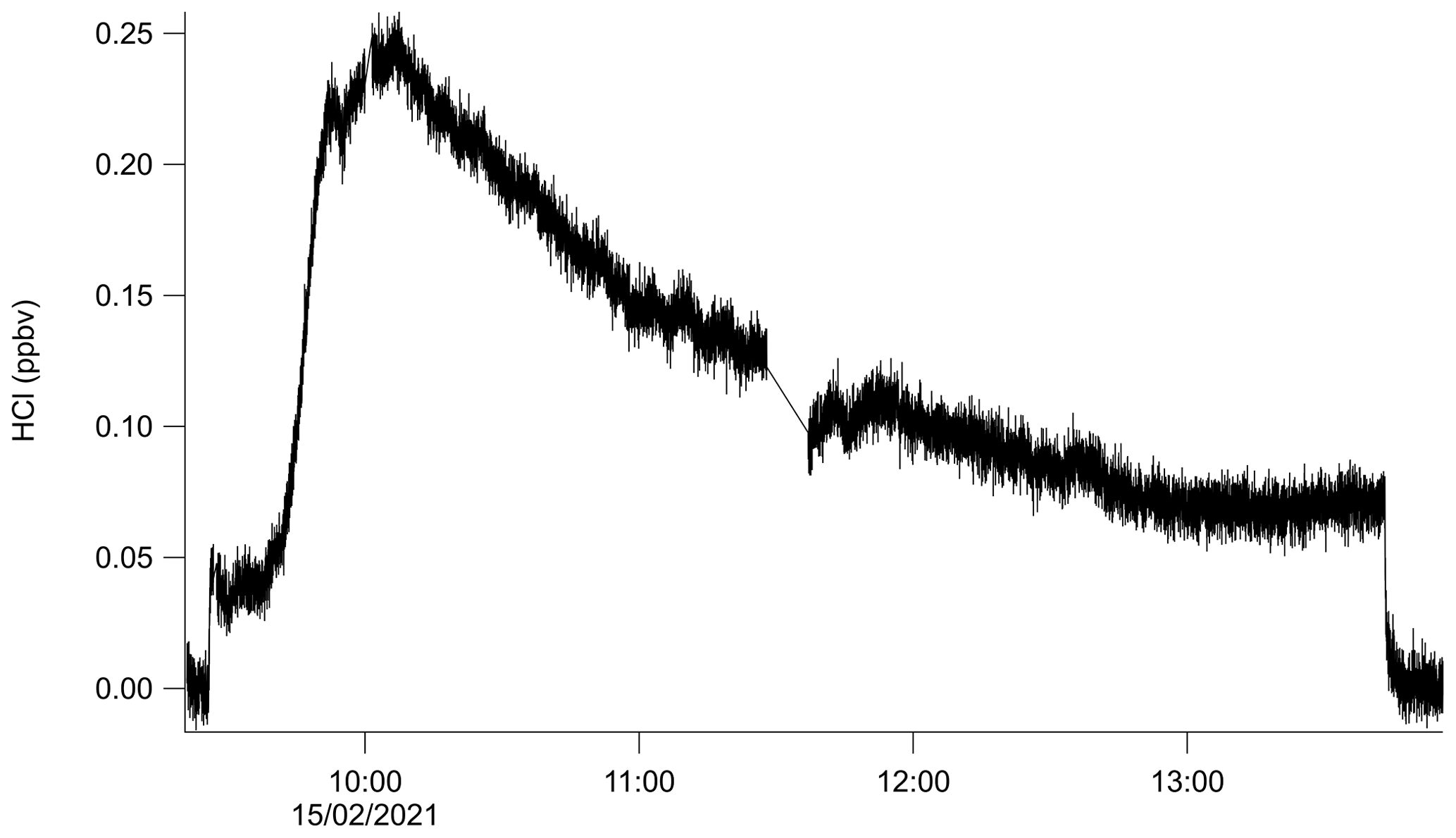
Figure 8Demonstration of the effects of 3.0 ppbv nitric acid addition to the passivated sample inlet flow at approximately 09:45 UTC.
There is no absorption band overlap between HNO3 and HCl in the analyzed spectral region, strongly indicating the observed increase in HCl signal occurred due to additional HCl molecules reaching the absorption cell. It is plausible this occurs because of interactions between HNO3 and surfaces where HCl may be adsorbed or with sampled particulates (although not in this specific case due to the particle-free air being used). One possible mechanism is that the HNO3 increases competition for sorption sites and ultimately replaces HCl on the surface. In this scenario, expected behavior would be a gradual increase in the background HCl signal as the stronger acid removes available sorption sites, and increased HCl throughput is achieved. A second mechanism would occur if water or particulate Cl− are present on instrument surfaces; here, the diffusion of the HNO3 into the water would cause acid displacement of HCl, as in Reaction (R2). If the strong acid flux were large enough, a sharp HCl signal increase (commensurate with the magnitude of available Cl−) would be anticipated from HCl off-gassing that would gradually recover as a new equilibrium is established. As seen in Fig. 8, it appears that a combination of these mechanisms is present. Once equilibrium had been established with addition of HNO3, flow from additional HNO3 permeation sources were added to the inertial inlet to observe whether additional HCl would be driven off (results not shown). However, each addition of HNO3 resulted in similar spikes and signal recoveries to elevated HCl background levels. As the sudden introduction of 3.0 ppbv HNO3 into the TILDAS inlet produced < 10 % of a signal response, it is likely a more gradual introduction of HNO3 would elicit a proportionally smaller HCl signal. Further, Fig. 8 was produced using an inertial inlet flow rate of 2.8 L min−1; these mechanisms are expected to be further reduced using faster-flow inlets (e.g., 12.7 L min−1), which would both reduce gas–surface interactions and make the mixing ratio transient proportionally smaller. In any case, this result demonstrates the importance of reducing the ability of HCl to stick to inlet and instrument surfaces.
While this interference was shown to be of potential significance in a laboratory context, in situ effects cannot be quantified without concurrent HNO3 (or proxy) observations. To this end, an examination of how HNO3 affects our method in a real-world context are further explored in Sect. 3.4.
3.4 Field sampling
Field observations for HCl-TILDAS were obtained during the summer 2021 OSCA campaign, hosted at the University of Manchester (Sect. 2.4; Fig. 9). These represent the second high-frequency tropospheric field measurement of HCl reported by optical techniques (Angelucci et al., 2021). For the period presented, ambient relative humidity ranged from 36 % to 98 %, and corresponded with average τe of 2.8 ± 0.3 s (τ90=7 ± 1 s). Because the inertial inlet used in this study had a flow rate of 3.7 L min−1, the expected 1/e residence time in the Herriott cell is approximately 1.5 s; these longer empirical instrument response timescales indicate incomplete passivation of inlet surfaces. Further, as discussed in Sect. 3.2.2, it is expected that the magnitude of the HCl measurements will be biased low by as much as 5.8 % in this campaign due to inlet surface losses, quantified through regular field additions of a HCl permeation standard (Fig. 7). Periods where the data spiked into negative values may have been caused by faulty blanks and are deemed to be below the instrument's 3σ limit of detection.
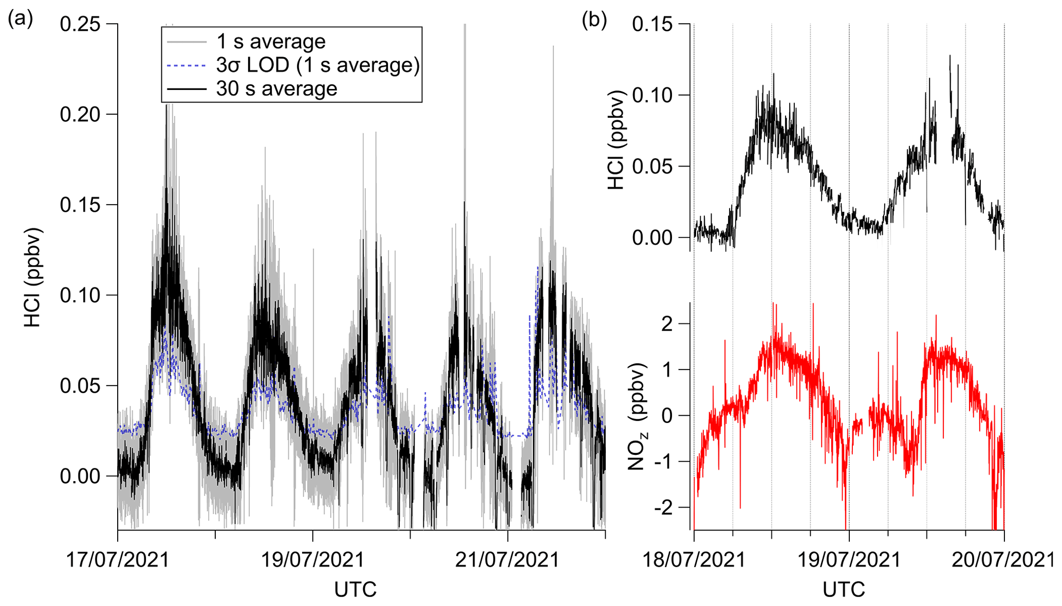
Figure 9Excerpted field data from the summer OSCA 2021 campaign. (a) Averaged time series during the final week of measurements, in which gray represents 1 s data collection frequency, the dashed blue line represents the 1 Hz 3σ limit of detection, and the black trace represents 30 s averages of these same HCl data. (b) Comparison of HCl time series (top) and concurrent NOz time series, with both averaged to 1 min. Gaps in data result from additions of high-concentration HCl standards that do not reflect ambient values. The increased noise in the data around these time periods is likely due to inlet effects following the HCl additions.
Additional sources of uncertainty may be introduced from plumes of HNO3 sampled by our inlet, as discussed in Sect. 3.3.2. While no direct HNO3 measurement was obtained during the OSCA campaign, NOz was used as an approximation, calculated from co-located NOx and NOy observations (NOz = NOy–NO–NO2) (Watson, 2022c, b). We note that this NOz measurement is highly uncertain due to the method of subtraction used to calculate NOz and the potential for other sources of NOz aside from HNO3 (San Martini et al., 2006) and is therefore used only for comparative purposes. For the period presented in Fig. 9b, a Pearson correlation coefficient (r) of 0.69 was found between HCl and NOz. Given both compounds ambient production pathways are expected to follow a photochemically driven diurnal cycle, this suggestion of linearity is not surprising. However, the profiles themselves differ, with changes in NOz lagging changes in HCl. For example, HCl mixing ratios begin to rise at 06:00 UTC on 18 July 2021, while NOz mixing ratios remain comparatively plateaued until 08:00 UTC, when it begins its rise. A similar pattern repeats on 19 July 2021, in which HCl mixing ratios begin rising just before 06:00 UTC, and NOz mixing ratios again do not increase until 08:00 UTC. The sharp increase in NOz mixing ratios after 08:00 UTC is not followed by an in-kind increase in HCl mixing ratios; if HNO3 were eliciting HCl within the sample inlet, it would be expected fluxes of HNO3 would precede or coincide with increases in HCl. As such, we do not believe HNO3 is a significant interference within our inlet for the period analyzed here.
To test the extent to which pCl− may repartition to HCl, a denuder was temporarily fitted in line to sample only pCl−; consequently, any HCl observed during the time period could be attributed to the repartitioning of pCl− within the TILDAS sample inlet (Fig. 10). To confirm the efficacy of removing HCl gas, cylinder additions that result in TILDAS-observed mixing ratios of 2.8, 35, and 69 ppbv were injected through the denuder for 60 s with no corresponding increase in TILDAS signal (Fig. 10c). For the period presented, HCl signal was seen to range between limits of detection to peaking at 53 pptv. ISORROPIA was used to test how much HCl may originate from pCl− in the conditions during the OSCA campaign, utilizing co-located measurements of total (gas + aerosol) concentrations of NH3 (using a Los Gatos Research ammonia analyzer) and HNO3 (as NOz) (Watson, 2022c, b, a) within the heated inlet system using the “forward” mode in ISORROPIA (no metals were included in these calculations). Based on these simulations, it was expected that the majority of pCl− would partition into the gas phase upon reaching thermal equilibrium in the sample inlet, leading to systematic errors of up to 40, 43, and 48 pptv at 308, 323, and 353 K, respectively. While the HCl signal did reach these values while the denuder was installed, no direct relationship was observed between the HCl signal and concurrent pCl− measurements (Fig. 10a, b). In particular, there are instances (e.g., between 12:00 and 15:00 UTC on 21 June 2021) where the available chlorine (calculated as the mixing ratio of chlorine if it were entirely released from particulates) is less than HCl observations. This may suggest a potential leak between the denuder and the inertial inlet that could allow a small volume of ambient air to contaminate the air sample, obfuscating accurate interpretation of these results. While a strong relationship was not observed between the pCl− and HCl signals (with denuder) in the period observed here, the ISORROPIA predictions emphasize that this is a significant possible source of positive error in HCl measurements whenever heated sample lines are used for HCl sampling in the presence of particulates.
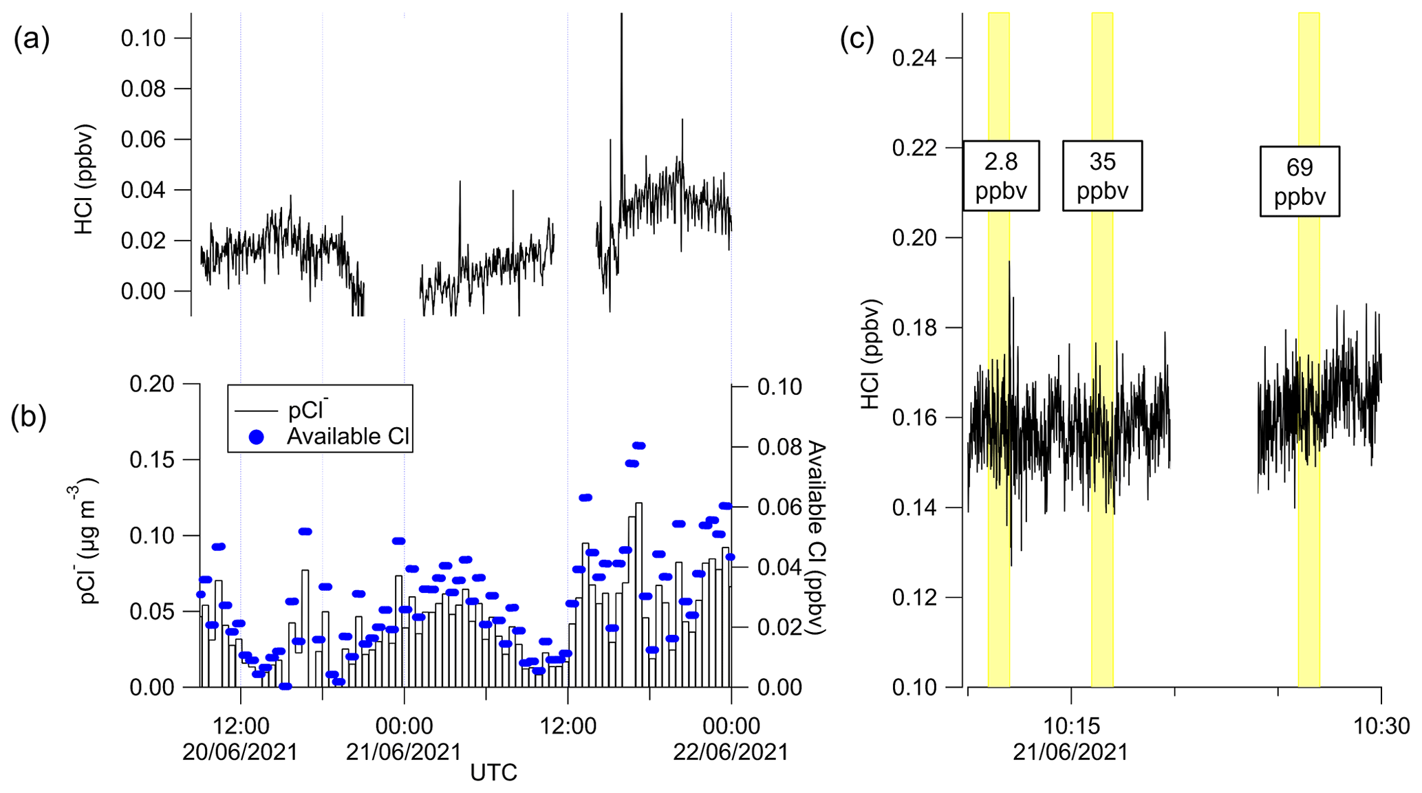
Figure 10Time series of (a) HCl when the denuder was installed on HCl TILDAS inlet in comparison with (b) pCl− observations. Available Cl was calculated by converting the pCl− concentrations into mixing ratios. (c) HCl cylinder additions were conducted (yellow shading) to verify the denuder was removing gas-phase HCl. The data in panel (c) have not been blank corrected or time averaged.
This work has demonstrated the viability of HCl-TILDAS for obtaining high-frequency ( Hz) observations of ambient HCl. The associated sampling method, involving a virtual impactor to avoid excess surface-mediated interactions with filters, as well as heat and chemical passivation to increase HCl throughput, was also shown to greatly improve instrument response to changes in HCl concentration (τ90≥1.15 s). However, there is room for further innovation in obviating the stickiness of HCl, including additional heating of sampling lines, minimizing pressure within the sampling line, and utilizing higher-flow inlets (e.g., ≥ 12 L min−1). The use of shorter inlet lines (< 3 m) operating at higher flow rates will additionally reduce sample air residence time in the inlet (≤ 0.54 s, as in this study), both reducing HCl–wall interactions and mitigating the likelihood of HCl partitioning out of particulates within the inlet. Introducing a temperature ramp to the inlet system after manual additions of high HCl mixing ratios may additionally reduce the amount of sorbed HCl available for acid displacement should strong acids be sampled under ambient conditions. The fast time responses to changes in HCl mixing ratios shown herein will be well suited for mobile sampling platforms, such as aircraft- or vehicle-based laboratories, in which both high temporal and spatial concentration variability are inherent. Finally, the potential for interferences from particulate chloride necessitates careful consideration regarding the method of obtaining background measurements. Regular installations of a denuder or incorporation of a denuder into a background mechanism would minimize the uncertainty presented.
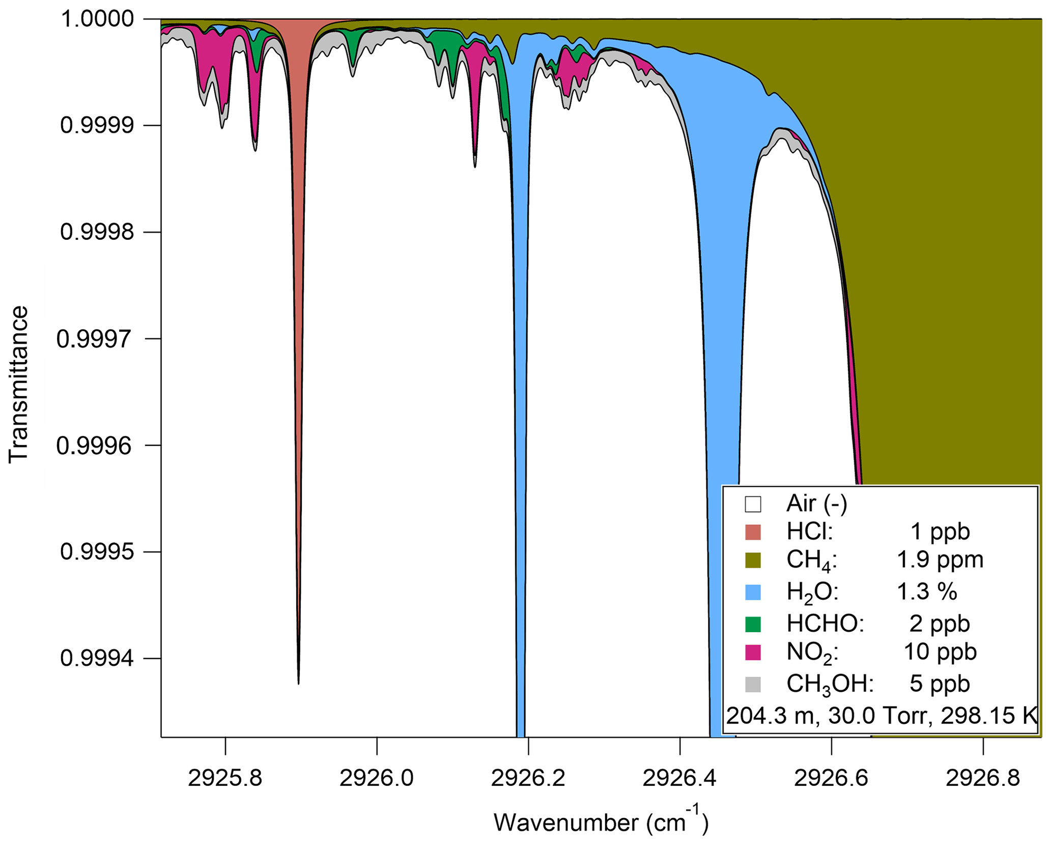
Figure A1HITRAN transmittance spectrum simulation demonstrating the separation of absorption peaks over the observed spectral window (2925.80 to 2926.75 cm−1).
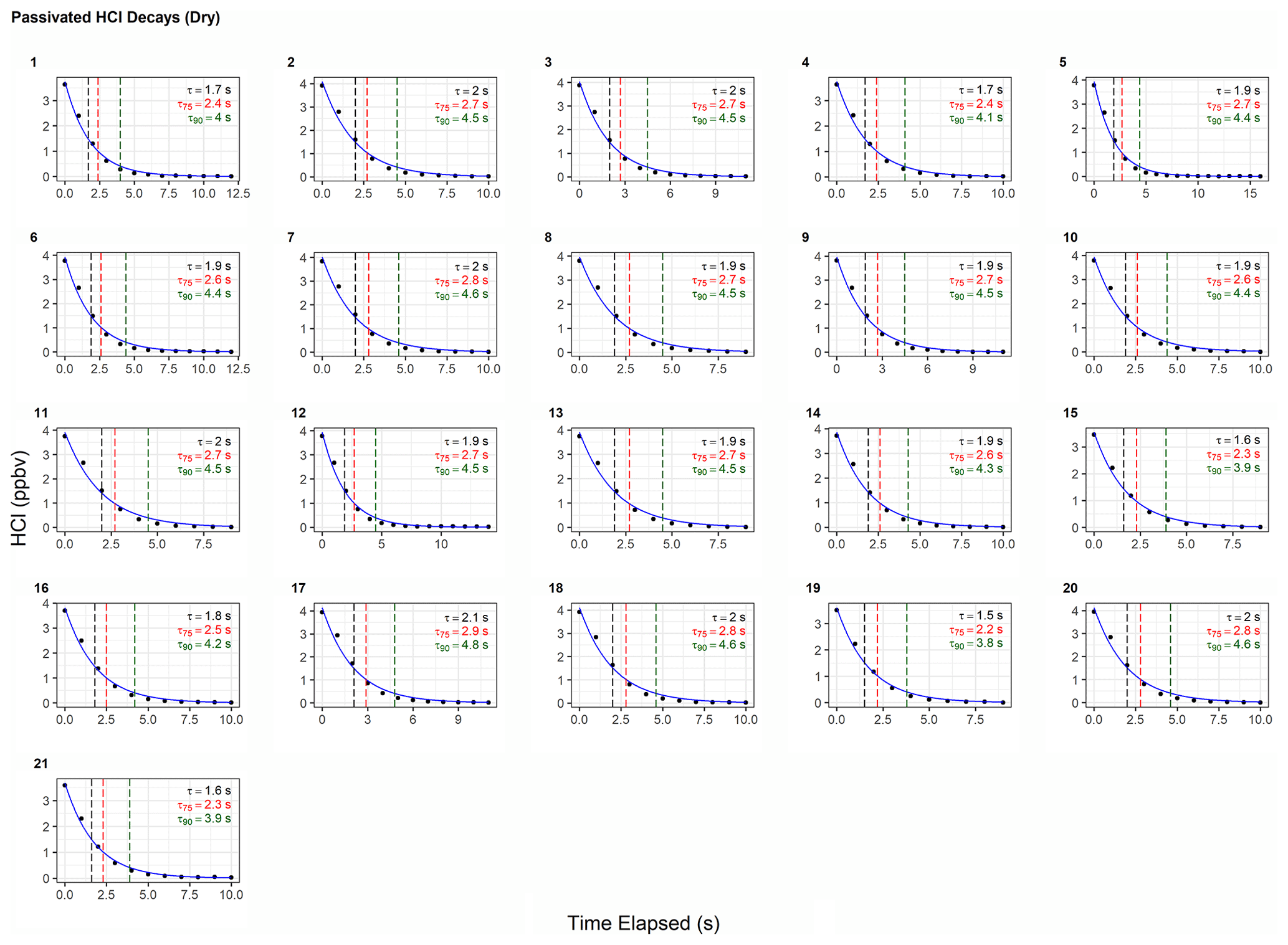
Figure A2Instrument response times to changes in HCl mixing ratios utilizing active passivation. Black dots represent observed data and are overlaid by the calculated single-exponential model (according to the terms listed in Table A1). Vertical hashed lines are placed on time elapsed corresponding to τe (black), τ75 (red), and τ90 (green).
Table A1Results for each model fit for determining the instrument response times under actively passivated conditions with the 2.8 L min−1 inertial inlet, corresponding to Fig. A2. Model parameters correspond to Eq. (1) in Sect. 2.6.2.
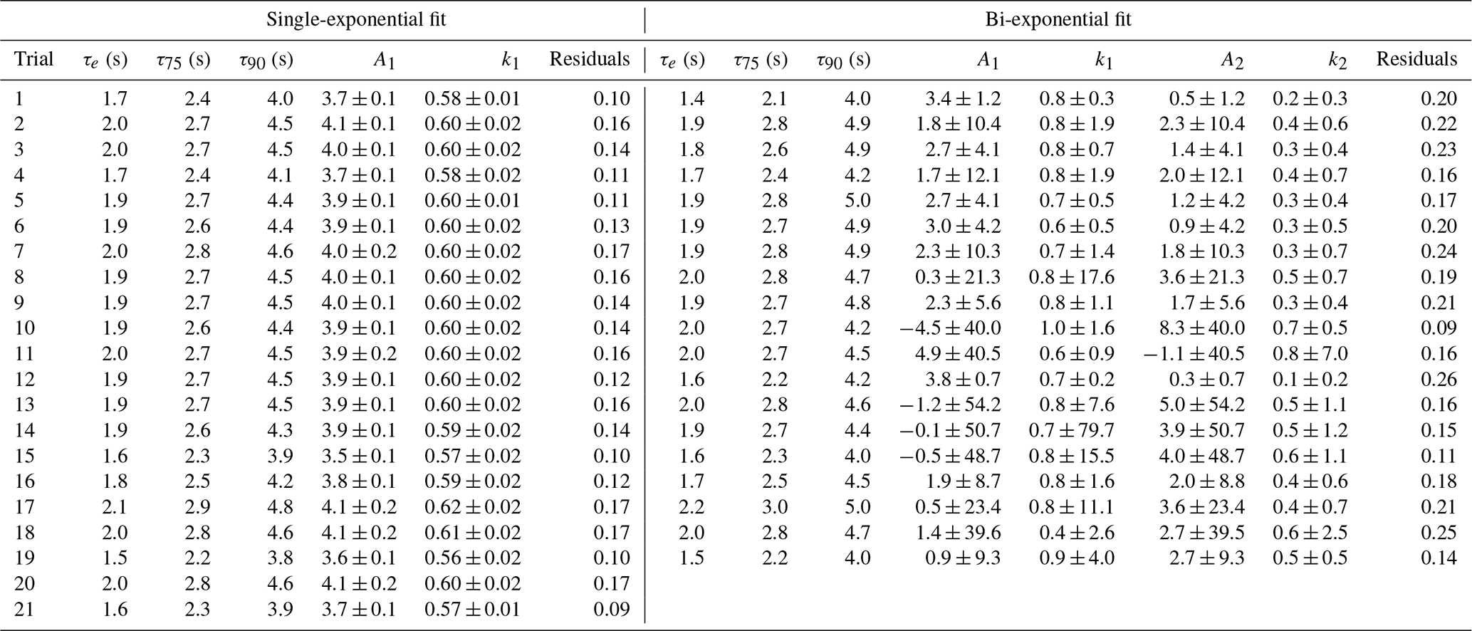
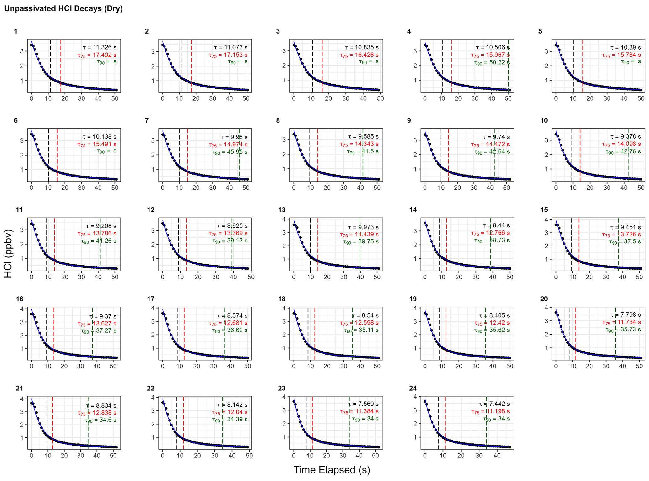
Figure A3Instrument response times to changes in HCl mixing ratios without active chemical passivation. Black dots represent observed data and are overlaid by the calculated bi-exponential model (according to the terms listed in Table A2). Vertical hashed lines are placed on time elapsed corresponding to τe (black), τ75 (red), and τ90 (green).
Table A2Results for each model fit for determining the instrument response times without use of active chemical passivation using the 2.8 L min−1 inertial inlet and corresponding to Fig. A3. Model parameters correspond to Eq. (1) in Sect. 2.6.2.
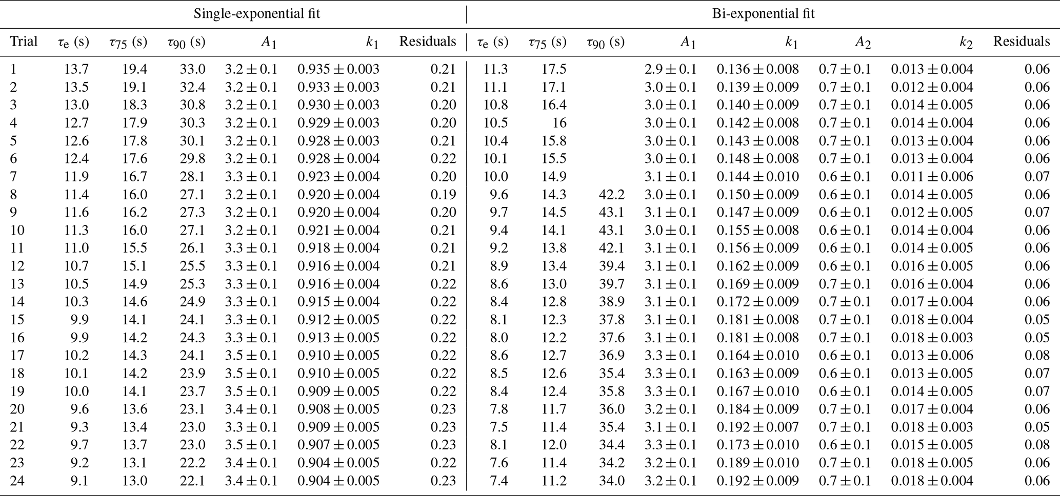

Figure A4Instrument response times to changes in HCl mixing ratios with active chemical passivation and a high-flow inertial inlet (12.7 L min−1). Black dots represent observed data and are overlaid by the calculated single exponential model (according to the terms listed in Table A3). Vertical hashed lines are placed on time elapsed corresponding to τe (black), τ75 (red), and τ90 (green).
Table A3Results for each model fit for determining the instrument response times under actively passivated conditions with the 12.7 L min−1 inertial inlet (Fig. A4). Model parameters correspond to Eq. (1) in Sect. 2.6.2.
Code used for this study can be obtained from the corresponding author upon request.
HCl data used for this study can be obtained from the corresponding author upon request. Particulate data used for ISORROPIA II simulations were obtained from Bandy et al. (2012), Lee and Young (2012), Crilley et al. (2017), Lee et al. (2021), and Watson (2022a). NO, NO2, and NOy data may be obtained from the Centre for Environmental Data Analysis website (Watson, 2022b, c).
SCH, JRR, CD, and TIY designed, built, and tested the HCl TILDAS at Aerodyne Research, Inc. SSB and PRV were involved in the initial HCl detector testing and supported the Aerodyne Research, Inc., instrument development. JWH and PME designed laboratory and field experiments, and JWH conducted laboratory and field experiments. SJA designed and constructed bespoke temperature-controlling units for the inertial inlet, the field inlet box, and permeation source ovens. JS performed ISORROPIA modeling experiments. MF provided NOx and NOy data and provided critical field support during the OSCA campaign. JWH prepared the manuscript, and all authors reviewed the manuscript.
The contact author has declared that none of the authors has any competing interests.
Publisher’s note: Copernicus Publications remains neutral with regard to jurisdictional claims in published maps and institutional affiliations.
We would like to thank the organizers of the OSCA Project for allowing our participation (NERC SPF OSCA project no. NE/T001917/1). The authors would also like to thank Abigail Mortimer, Stuart Murray, Chris Rhodes, and Mark Roper of the University of York chemistry workshops, as well as Christopher Anthony, for technical support, and Stuart Lacy of the University of York Wolfson Atmospheric Chemistry Laboratory for data analysis software support. Further, the authors thank Michael Agnese and Michael Moore for TILDAS technical support. The authors would like to acknowledge the efforts Conner Daube made in testing configuration and sampling procedures on the companion HCl instrument. The authors would also like to acknowledge the spectroscopic analysis performed by Barry McManus to diagnose nonideal noise sources and design alignment optimizations. In addition, the authors thank James Lee, Will Drysdale, and Katie Read for their support in laboratory experiments involving HNO3 quantification.
This research has been supported by the European Research Council (H2020, grant no. ERC-StG 802685). We would also like to thank the NOAA Small Business Innovation Research Program (WC-133R-17-CN-0092) for funding the HCl instrument development work performed by Aerodyne Research, Inc.
This paper was edited by Mingjin Tang and reviewed by three anonymous referees.
Abbatt, J., Oldridge, N., Symington, A., Chukalovskiy, V., McWhinney, R. D., Sjostedt, S., and Cox, R. A.: Release of Gas-Phase Halogens by Photolytic Generation of OH in Frozen Halide-Nitrate Solutions: An Active Halogen Formation Mechanism?, J. Phys. Chem. A, 114, 6527–6533, https://doi.org/10.1021/jp102072t, 2010.
Allan, W., Lowe, D. C., and Cainey, J. M.: Active chlorine in the remote marine boundary layer: Modeling anomalous measurements of δ13C in methane, Geophys. Res. Lett., 28, 3239–3242, https://doi.org/10.1029/2001GL013064, 2001.
Angelucci, A. A., Furlani, T. C., Wang, X., Jacob, D. J., VandenBoer, T. C., and Young, C. J.: Understanding Sources of Atmospheric Hydrogen Chloride in Coastal Spring and Continental Winter, ACS Earth Space Chem., 5, 2507–2516, https://doi.org/10.1021/acsearthspacechem.1c00193, 2021.
Atkinson, R., Baulch, D. L., Cox, R. A., Crowley, J. N., Hampson, R. F., Hynes, R. G., Jenkin, M. E., Rossi, M. J., Troe, J., and IUPAC Subcommittee: Evaluated kinetic and photochemical data for atmospheric chemistry: Volume II – gas phase reactions of organic species, Atmos. Chem. Phys., 6, 3625–4055, https://doi.org/10.5194/acp-6-3625-2006, 2006.
Atkinson, R., Baulch, D. L., Cox, R. A., Crowley, J. N., Hampson, R. F., Hynes, R. G., Jenkin, M. E., Rossi, M. J., and Troe, J.: Evaluated kinetic and photochemical data for atmospheric chemistry: Volume III – gas phase reactions of inorganic halogens, Atmos. Chem. Phys., 7, 981–1191, https://doi.org/10.5194/acp-7-981-2007, 2007.
Bandy, B., Faloon, K., Finessi, E., Lee, J. D., Leigh, R. J., Liu, D., Monks, P. S., Oram, D. E., Visser, S., Whitehead, J., and Young, D.: ClearfLo: IOP Summer Atmospheric Chemistry and meteorology measurements and NAME Airmass Footprint dispersion model output at North Kensington, London, NCAS British Atmospheric Data Centre [data set], https://catalogue.ceda.ac.uk/uuid/4c35e63d6507408d96e4af3dce410e3d (last access: 19 October 2022), 2012.
Behnke, W. and Zetzsch, C.: Heterogeneous photochemical formation of Cl atoms from NaCl aerosol, NOx and ozone, J. Aerosol Sci., 21, S229–S232, https://doi.org/10.1016/0021-8502(90)90226-N, 1990.
Behnke, W., Krüger, H.-U., Scheer, V., and Zetzsch, C.: Formation of ClNO2 and hono in the presence of NO2, O3 and wet NaCl aerosol, J. Aerosol Sci., 23, 933–936, https://doi.org/10.1016/0021-8502(92)90565-D, 1992.
Behnke, W., George, C., Scheer, V., and Zetzsch, C.: Production and decay of ClNO2 from the reaction of gaseous N2O5 with NaCl solution: Bulk and aerosol experiments, J. Geophys. Res.-Atmos., 102, 3795–3804, https://doi.org/10.1029/96JD03057, 1997.
Beichert, P. and Finlayson-Pitts, B. J.: Knudsen Cell Studies of the Uptake of Gaseous HNO3 and Other Oxides of Nitrogen on Solid NaCl: The Role of Surface-Adsorbed Water, J. Phys. Chem., 100, 15218–15228, https://doi.org/10.1021/jp960925u, 1996.
Brimblecombe, P. and Clegg, S. L.: The solubility and behaviour of acid gases in the marine aerosol, J. Atmos. Chem., 7, 1–18, https://doi.org/10.1007/BF00048251, 1988.
Buck, R. C., Franklin, J., Berger, U., Conder, J. M., Cousins, I. T., de Voogt, P., Jensen, A. A., Kannan, K., Mabury, S. A., and van Leeuwen, S. P.: Perfluoroalkyl and polyfluoroalkyl substances in the environment: Terminology, classification, and origins, Integr. Environ. Assess. Manag., 7, 513–541, https://doi.org/10.1002/ieam.258, 2011.
Burkholder, J. B., Sander, S. P., Abbatt, J., Barker, J. R., Huie, R. E., Kolb, C. E., Kurylo, M. J., Orkin, V. L., Wilmouth, D. M., and Wine, P. H.: Chemical Kinetics and Photochemical Data for Use in Atmospheric Studies, Evaluation No. 18, JPL Publication 15-10., Jet Propulsion Laboratory, Pasadena, 2015.
Clegg, S. L. and Brimblecombe, P.: The dissociation constant and henry's law constant of HCl in aqueous solution, Atmos. Environ., 1967, 2483–2485, https://doi.org/10.1016/0004-6981(86)90079-X, 1986.
Crilley, L. R., Lucarelli, F., Bloss, W. J., Harrison, R. M., Beddows, D. C., Calzolai, G., Nava, S., Valli, G., Bernardoni, V., and Vecchi, R.: Source apportionment of fine and coarse particles at a roadside and urban background site in London during the 2012 summer ClearfLo campaign, Environ. Pollut., 220, 766–778, https://doi.org/10.1016/j.envpol.2016.06.002, 2017.
Crisp, T. A., Lerner, B. M., Williams, E. J., Quinn, P. K., Bates, T. S., and Bertram, T. H.: Observations of gas phase hydrochloric acid in the polluted marine boundary layer, J. Geophys. Res.-Atmos., 119, 6897–6915, https://doi.org/10.1002/2013JD020992, 2014.
Eger, P. G., Helleis, F., Schuster, G., Phillips, G. J., Lelieveld, J., and Crowley, J. N.: Chemical ionization quadrupole mass spectrometer with an electrical discharge ion source for atmospheric trace gas measurement, Atmos. Meas. Tech., 12, 1935–1954, https://doi.org/10.5194/amt-12-1935-2019, 2019a.
Eger, P. G., Friedrich, N., Schuladen, J., Shenolikar, J., Fischer, H., Tadic, I., Harder, H., Martinez, M., Rohloff, R., Tauer, S., Drewnick, F., Fachinger, F., Brooks, J., Darbyshire, E., Sciare, J., Pikridas, M., Lelieveld, J., and Crowley, J. N.: Shipborne measurements of ClNO2 in the Mediterranean Sea and around the Arabian Peninsula during summer, Atmospheric Chem. Phys., 19, 12121–12140, https://doi.org/10.5194/acp-19-12121-2019, 2019b.
Ellis, R. A., Murphy, J. G., Pattey, E., van Haarlem, R., O'Brien, J. M., and Herndon, S. C.: Characterizing a Quantum Cascade Tunable Infrared Laser Differential Absorption Spectrometer (QC-TILDAS) for measurements of atmospheric ammonia, Atmos. Meas. Tech., 3, 397–406, https://doi.org/10.5194/amt-3-397-2010, 2010.
Erickson, D. J., Seuzaret, C., Keene, W. C., and Gong, S. L.: A general circulation model based calculation of HCl and ClNO2 production from sea salt dechlorination: Reactive Chlorine Emissions Inventory, J. Geophys. Res.-Atmos., 104, 8347–8372, https://doi.org/10.1029/98JD01384, 1999.
Fickert, S., Adams, J. W., and Crowley, J. N.: Activation of Br2 and BrCl via uptake of HOBr onto aqueous salt solutions, J. Geophys. Res.-Atmos., 104, 23719–23727, https://doi.org/10.1029/1999JD900359, 1999.
Fountoukis, C. and Nenes, A.: ISORROPIA II: a computationally efficient thermodynamic equilibrium model for K+–Ca2+–Mg2+–NH–Na+–SO–NO3–Cl–H2O aerosols, Atmos. Chem. Phys., 7, 4639–4659, https://doi.org/10.5194/acp-7-4639-2007, 2007.
Frinak, E. K. and Abbatt, J. P. D.: Br2 Production from the Heterogeneous Reaction of Gas-Phase OH with Aqueous Salt Solutions: Impacts of Acidity, Halide Concentration, and Organic Surfactants, J. Phys. Chem. A, 110, 10456–10464, https://doi.org/10.1021/jp063165o, 2006.
Fu, X., Wang, T., Wang, S., Zhang, L., Cai, S., Xing, J., and Hao, J.: Anthropogenic Emissions of Hydrogen Chloride and Fine Particulate Chloride in China, Environ. Sci. Technol., 52, 1644–1654, https://doi.org/10.1021/acs.est.7b05030, 2018.
Furlani, T. C., Veres, P. R., Dawe, K. E. R., Neuman, J. A., Brown, S. S., VandenBoer, T. C., and Young, C. J.: Validation of a new cavity ring-down spectrometer for measuring tropospheric gaseous hydrogen chloride, Atmos. Meas. Tech., 14, 5859–5871, https://doi.org/10.5194/amt-14-5859-2021, 2021.
Gordon, I. E., Rothman, L. S., Hill, C., Kochanov, R. V., Tan, Y., Bernath, P. F., Birk, M., Boudon, V., Campargue, A., Chance, K. V., Drouin, B. J., Flaud, J.-M., Gamache, R. R., Hodges, J. T., Jacquemart, D., Perevalov, V. I., Perrin, A., Shine, K. P., Smith, M.-A. H., Tennyson, J., Toon, G. C., Tran, H., Tyuterev, V. G., Barbe, A., Császár, A. G., Devi, V. M., Furtenbacher, T., Harrison, J. J., Hartmann, J.-M., Jolly, A., Johnson, T. J., Karman, T., Kleiner, I., Kyuberis, A. A., Loos, J., Lyulin, O. M., Massie, S. T., Mikhailenko, S. N., Moazzen-Ahmadi, N., Müller, H. S. P., Naumenko, O. V., Nikitin, A. V., Polyansky, O. L., Rey, M., Rotger, M., Sharpe, S. W., Sung, K., Starikova, E., Tashkun, S. A., Auwera, J. V., Wagner, G., Wilzewski, J., Wcisło, P., Yu, S., and Zak, E. J.: The HITRAN2016 molecular spectroscopic database, J. Quant. Spectrosc. Ra. Transf., 203, 3–69, https://doi.org/10.1016/j.jqsrt.2017.06.038, 2017.
Graedel, T. E. and Keene, W. C.: Tropospheric budget of reactive chlorine, Global Biogeochem. Cy., 9, 47–77, https://doi.org/10.1029/94GB03103, 1995.
Graedel, T. E. and Keene, W. C.: The Budget and Cycle of Earth's Natural Chlorine, Pure Appl. Chem., 68, 1689–1697, https://doi.org/10.1351/pac199668091689, 1996.
Guelachvili, G., Niay, P., and Bernage, P.: Infrared bands of HCl and DCl by Fourier transform spectroscopy: Dunham coefficients for HCl, DCl, and TCl, J. Mol. Spectrosc., 85, 271–281, https://doi.org/10.1016/0022-2852(81)90200-9, 1981.
Hagen, C. L., Lee, B. C., Franka, I. S., Rath, J. L., VandenBoer, T. C., Roberts, J. M., Brown, S. S., and Yalin, A. P.: Cavity ring-down spectroscopy sensor for detection of hydrogen chloride, Atmos. Meas. Tech., 7, 345–357, https://doi.org/10.5194/amt-7-345-2014, 2014.
Harris, G. W., Klemp, D., and Zenker, T.: An upper limit on the HCl near-surface mixing ratio over the Atlantic measured using TDLAS, J. Atmos. Chem., 15, 327–332, https://doi.org/10.1007/BF00115402, 1992.
Haskins, J. D., Jaeglé, L., Shah, V., Lee, B. H., Lopez-Hilfiker, F. D., Campuzano-Jost, P., Schroder, J. C., Day, D. A., Guo, H., Sullivan, A. P., Weber, R., Dibb, J., Campos, T., Jimenez, J. L., Brown, S. S., and Thornton, J. A.: Wintertime Gas-Particle Partitioning and Speciation of Inorganic Chlorine in the Lower Troposphere Over the Northeast United States and Coastal Ocean, J. Geophys. Res.-Atmos., 123, 12897–12916, https://doi.org/10.1029/2018JD028786, 2018.
Huffman, J. A., Docherty, K. S., Aiken, A. C., Cubison, M. J., Ulbrich, I. M., DeCarlo, P. F., Sueper, D., Jayne, J. T., Worsnop, D. R., Ziemann, P. J., and Jimenez, J. L.: Chemically-resolved aerosol volatility measurements from two megacity field studies, Atmos. Chem. Phys., 9, 7161–7182, https://doi.org/10.5194/acp-9-7161-2009, 2009.
Jahn, L. G., Wang, D. S., Dhulipala, S. V., and Ruiz, L. H.: Gas-Phase Chlorine Radical Oxidation of Alkanes: Effects of Structural Branching, NOx, and Relative Humidity Observed during Environmental Chamber Experiments, J. Phys. Chem. A, 125, 7303–7317, https://doi.org/10.1021/acs.jpca.1c03516, 2021.
Keene, W. C., Khalil, M. A. K., Erickson, D. J., McCulloch, A., Graedel, T. E., Lobert, J. M., Aucott, M. L., Gong, S. L., Harper, D. B., Kleiman, G., Midgley, P., Moore, R. M., Seuzaret, C., Sturges, W. T., Benkovitz, C. M., Koropalov, V., Barrie, L. A., and Li, Y. F.: Composite global emissions of reactive chlorine from anthropogenic and natural sources: Reactive Chlorine Emissions Inventory, J. Geophys. Res.-Atmos., 104, 8429–8440, https://doi.org/10.1029/1998JD100084, 1999.
Knipping, E. M., Lakin, M. J., Foster, K. L., Jungwirth, P., Tobias, D. J., Gerber, R. B., Dabdub, D., and Finlayson-Pitts, B. J.: Experiments and Simulations of Ion-Enhanced Interfacial Chemistry on Aqueous NaCl Aerosols, Science, 288, 301–306, https://doi.org/10.1126/science.288.5464.301, 2000.
Laasonen, K. E. and Klein, M. L.: Ab Initio Study of Aqueous Hydrochloric Acid, J. Phys. Chem. A, 101, 98–102, https://doi.org/10.1021/jp962513r, 1997.
Laskin, A., Moffet, R. C., Gilles, M. K., Fast, J. D., Zaveri, R. A., Wang, B., Nigge, P., and Shutthanandan, J.: Tropospheric chemistry of internally mixed sea salt and organic particles: Surprising reactivity of NaCl with weak organic acids, J. Geophys. Res.-Atmos., 117, D15302, https://doi.org/10.1029/2012JD017743, 2012.
Lee, J. D. and Young, D.: ClearfLo: Atmospheric Chemistry measurements and NAME Airmass Footprint dispersion model output at North Kensington, London, NCAS British Atmospheric Data Centre [data set], https://catalogue.ceda.ac.uk/uuid/6a5f9eedd68f43348692b3bace3eba45 (last access: 19 October 2022), 2012.
Lee, B. H., Lopez-Hilfiker, F. D., Schroder, J. C., Campuzano-Jost, P., Jimenez, J. L., McDuffie, E. E., Fibiger, D. L., Veres, P. R., Brown, S. S., Campos, T. L., Weinheimer, A. J., Flocke, F. F., Norris, G., O'Mara, K., Green, J. R., Fiddler, M. N., Bililign, S., Shah, V., Jaeglé, L., and Thornton, J. A.: Airborne Observations of Reactive Inorganic Chlorine and Bromine Species in the Exhaust of Coal-Fired Power Plants, J. Geophys. Res.-Atmos., 123, 11225–11237, https://doi.org/10.1029/2018JD029284, 2018.
Lee, J. D., Herndon, S., Zotter, P., Visser, S., Bandy, B., Oram, D., Laufs, S., Hopkins, J. R., and Fleming, Z. L.: ClearfLo: IOP Winter atmospheric chemistry and meteorology measurements and NAME Airmass Footprint dispersion model output across London sites, NERC EDS Centre for Environmental Data Analysis [data set], https://catalogue.ceda.ac.uk/uuid/ba8180a9876a4ef1a127046a673d8864 (last access: 19 October 2022), 2021.
Li, G., Gordon, I. E., Bernath, P. F., and Rothman, L. S.: Direct fit of experimental ro-vibrational intensities to the dipole moment function: Application to HCl, J. Quant. Spectrosc. Ra. Transf., 112, 1543–1550, https://doi.org/10.1016/j.jqsrt.2011.03.014, 2011.
Li, G., Gordon, I. E., Hajigeorgiou, P. G., Coxon, J. A., and Rothman, L. S.: Reference spectroscopic data for hydrogen halides, Part II: The line lists, J. Quant. Spectrosc. Ra. Transf., 130, 284–295, https://doi.org/10.1016/j.jqsrt.2013.07.019, 2013.
Liao, J., Huey, L. G., Liu, Z., Tanner, D. J., Cantrell, C. A., Orlando, J. J., Flocke, F. M., Shepson, P. B., Weinheimer, A. J., Hall, S. R., Ullmann, K., Beine, H. J., Wang, Y., Ingall, E. D., Stephens, C. R., Hornbrook, R. S., Apel, E. C., Riemer, D., Fried, A., Mauldin Iii, R. L., Smith, J. N., Staebler, R. M., Neuman, J. A., and Nowak, J. B.: High levels of molecular chlorine in the Arctic atmosphere, Nat. Geosci., 7, 91–94, https://doi.org/10.1038/ngeo2046, 2014.
Liu, X., Deming, B., Pagonis, D., Day, D. A., Palm, B. B., Talukdar, R., Roberts, J. M., Veres, P. R., Krechmer, J. E., Thornton, J. A., de Gouw, J. A., Ziemann, P. J., and Jimenez, J. L.: Effects of gas–wall interactions on measurements of semivolatile compounds and small polar molecules, Atmos. Meas. Tech., 12, 3137–3149, https://doi.org/10.5194/amt-12-3137-2019, 2019.
Marcy, T. P., Fahey, D. W., Gao, R. S., Popp, P. J., Richard, E. C., Thompson, T. L., Rosenlof, K. H., Ray, E. A., Salawitch, R. J., Atherton, C. S., Bergmann, D. J., Ridley, B. A., Weinheimer, A. J., Loewenstein, M., Weinstock, E. M., and Mahoney, M. J.: Quantifying Stratospheric Ozone in the Upper Troposphere with in Situ Measurements of HCl, Science, 304, 261–265, https://doi.org/10.1126/science.1093418, 2004.
McCulloch, A., Aucott, M. L., Benkovitz, C. M., Graedel, T. E., Kleiman, G., Midgley, P. M., and Li, Y.-F.: Global emissions of hydrogen chloride and chloromethane from coal combustion, incineration and industrial activities: Reactive Chlorine Emissions Inventory, J. Geophys. Res.-Atmos., 104, 8391–8403, https://doi.org/10.1029/1999JD900025, 1999.
McManus, J. B., Zahniser, M. S., and Nelson, D. D.: Dual quantum cascade laser trace gas instrument with astigmatic Herriott cell at high pass number, Appl. Opt., 50, A74, https://doi.org/10.1364/AO.50.000A74, 2011.
McManus, J. B., Zahniser, M. S., Nelson, D. D., Shorter, J. H., Herndon, S. C., Jervis, D., Agnese, M., McGovern, R., Yacovitch, T. I., and Roscioli, J. R.: Recent progress in laser-based trace gas instruments: performance and noise analysis, Appl. Phys. B, 119, 203–218, https://doi.org/10.1007/s00340-015-6033-0, 2015.
Neuman, J. A., Huey, L. G., Ryerson, T. B., and Fahey, D. W.: Study of Inlet Materials for Sampling Atmospheric Nitric Acid, Environ. Sci. Technol., 33, 1133–1136, https://doi.org/10.1021/es980767f, 1999.
Osthoff, H. D., Roberts, J. M., Ravishankara, A. R., Williams, E. J., Lerner, B. M., Sommariva, R., Bates, T. S., Coffman, D., Quinn, P. K., Dibb, J. E., Stark, H., Burkholder, J. B., Talukdar, R. K., Meagher, J., Fehsenfeld, F. C., and Brown, S. S.: High levels of nitryl chloride in the polluted subtropical marine boundary layer, Nat. Geosci., 1, 324–328, https://doi.org/10.1038/ngeo177, 2008.
Oum, K. W., Lakin, M. J., DeHaan, D. O., Brauers, T., and Finlayson-Pitts, B. J.: Formation of Molecular Chlorine from the Photolysis of Ozone and Aqueous Sea-Salt Particles, Science, 279, 74–76, https://doi.org/10.1126/science.279.5347.74, 1998.
Pollack, I. B., Lindaas, J., Roscioli, J. R., Agnese, M., Permar, W., Hu, L., and Fischer, E. V.: Evaluation of ambient ammonia measurements from a research aircraft using a closed-path QC-TILDAS operated with active continuous passivation, Atmos. Meas. Tech., 12, 3717–3742, https://doi.org/10.5194/amt-12-3717-2019, 2019.
Pszenny, A. A. P., Fischer, E. V., Russo, R. S., Sive, B. C., and Varner, R. K.: Estimates of Cl atom concentrations and hydrocarbon kinetic reactivity in surface air at Appledore Island, Maine (USA), during International Consortium for Atmospheric Research on Transport and Transformation/Chemistry of Halogens at the Isles of Shoals, J. Geophys. Res.-Atmos., 112, D10S13, https://doi.org/10.1029/2006JD007725, 2007.
R Core Team: R: A language and environment for statistical computing. R Foundation for Statistical Computing [software], https://www.R-project.org/ (last access: 8 February 2022), 2021.
Ren, X., Sun, R., Chi, H.-H., Meng, X., Li, Y., and Levendis, Y. A.: Hydrogen chloride emissions from combustion of raw and torrefied biomass, Fuel, 200, 37–46, https://doi.org/10.1016/j.fuel.2017.03.040, 2017.
Roberts, J. M., Veres, P., Warneke, C., Neuman, J. A., Washenfelder, R. A., Brown, S. S., Baasandorj, M., Burkholder, J. B., Burling, I. R., Johnson, T. J., Yokelson, R. J., and de Gouw, J.: Measurement of HONO, HNCO, and other inorganic acids by negative-ion proton-transfer chemical-ionization mass spectrometry (NI-PT-CIMS): application to biomass burning emissions, Atmos. Meas. Tech., 3, 981–990, https://doi.org/10.5194/amt-3-981-2010, 2010.
Roscioli, J. R., Zahniser, M. S., Nelson, D. D., Herndon, S. C., and Kolb, C. E.: New Approaches to Measuring Sticky Molecules: Improvement of Instrumental Response Times Using Active Passivation, J. Phys. Chem. A, 120, 1347–1357, https://doi.org/10.1021/acs.jpca.5b04395, 2016.
RStudio Team: RStudio: Integrated Development for R, RStudio, PBC [software], http://www.rstudio.com/ (last access: last access: 8 February 2022), 2021.
Saliba, N. A., Yang, H., and Finlayson-Pitts, B. J.: Reaction of Gaseous Nitric Oxide with Nitric Acid on Silica Surfaces in the Presence of Water at Room Temperature, J. Phys. Chem. A, 105, 10339–10346, https://doi.org/10.1021/jp012330r, 2001.
San Martini, F. M., Dunlea, E. J., Grutter, M., Onasch, T. B., Jayne, J. T., Canagaratna, M. R., Worsnop, D. R., Kolb, C. E., Shorter, J. H., Herndon, S. C., Zahniser, M. S., Ortega, J. M., McRae, G. J., Molina, L. T., and Molina, M. J.: Implementation of a Markov Chain Monte Carlo method to inorganic aerosol modeling of observations from the MCMA-2003 campaign – Part I: Model description and application to the La Merced site, Atmos. Chem. Phys., 6, 4867–4888, https://doi.org/10.5194/acp-6-4867-2006, 2006.
Scott, D. C., Herman, R. L., Webster, C. R., May, R. D., Flesch, G. J., and Moyer, E. J.: Airborne Laser Infrared Absorption Spectrometer (ALIAS-II) for in situ atmospheric measurements of N2O, CH4, CO, HCL, and NO2 from balloon or remotely piloted aircraft platforms, Appl. Opt., 38, 4609–4622, https://doi.org/10.1364/AO.38.004609, 1999.
Simpson, W. R., Brown, S. S., Saiz-Lopez, A., Thornton, J. A., and von Glasow, R.: Tropospheric Halogen Chemistry: Sources, Cycling, and Impacts, Chem. Rev., 115, 4035–4062, https://doi.org/10.1021/cr5006638, 2015.
Singh, H. B., Gregory, G. L., Anderson, B., Browell, E., Sachse, G. W., Davis, D. D., Crawford, J., Bradshaw, J. D., Talbot, R., Blake, D. R., Thornton, D., Newell, R., and Merrill, J.: Low ozone in the marine boundary layer of the tropical Pacific Ocean: Photochemical loss, chlorine atoms, and entrainment, J. Geophys. Res.-Atmos., 101, 1907–1917, https://doi.org/10.1029/95JD01028, 1996.
Sumner, A. L., Menke, E. J., Dubowski, Y., Newberg, J. T., Penner, R. M., Hemminger, J. C., Wingen, L. M., Brauers, T., and Finlayson-Pitts, B. J.: The nature of water on surfaces of laboratory systems and implications for heterogeneous chemistry in the troposphere, Phys. Chem. Chem. Phys., 6, 604–613, https://doi.org/10.1039/B308125G, 2004.
Tao, Y., VandenBoer, T. C., Veres, P. R., Warneke, C., de Gouw, J. A., Weber, R. J., Markovic, M. Z., Zhao, Y., Baker, K. R., Kelly, J. T., Murphy, J. G., Young, C. J., and Roberts, J. M.: Hydrogen Chloride (HCl) at Ground Sites During CalNex 2010 and Insight Into Its Thermodynamic Properties, J. Geophys. Res.-Atmos., 127, e2021JD036062, https://doi.org/10.1029/2021JD036062, 2022.
Toth, R. A., Hunt, R. H., and Plyler, E. K.: Line strengths, line widths, and dipole moment function for HCl, J. Mol. Spectrosc., 35, 110–126, https://doi.org/10.1016/0022-2852(70)90169-4, 1970.
Tuckermann, M., Ackermann, R., Gölz, C., Lorenzen-Schmidt, H., Senne, T., Stutz, J., Trost, B., Unold, W., and Platt, U.: DOAS-observation of halogen radical-catalysed arctic boundary layer ozone destruction during the ARCTOC-campaigns 1995 and 1996 in Ny-Ålesund, Spitsbergen, Tellus B Chem. Phys. Meteorol., 49, 533–555, https://doi.org/10.3402/tellusb.v49i5.16005, 1997.
Veres, P., Roberts, J. M., Warneke, C., Welsh-Bon, D., Zahniser, M., Herndon, S., Fall, R., and de Gouw, J.: Development of negative-ion proton-transfer chemical-ionization mass spectrometry (NI-PT-CIMS) for the measurement of gas-phase organic acids in the atmosphere, Int. J. Mass Spectrom., 274, 48–55, https://doi.org/10.1016/j.ijms.2008.04.032, 2008.
von Glasow, R., Bobrowski, N., and Kern, C.: The effects of volcanic eruptions on atmospheric chemistry, Chem. Geol., 263, 131–142, https://doi.org/10.1016/j.chemgeo.2008.08.020, 2009.
Wang, X., Jacob, D. J., Eastham, S. D., Sulprizio, M. P., Zhu, L., Chen, Q., Alexander, B., Sherwen, T., Evans, M. J., Lee, B. H., Haskins, J. D., Lopez-Hilfiker, F. D., Thornton, J. A., Huey, G. L., and Liao, H.: The role of chlorine in global tropospheric chemistry, Atmos. Chem. Phys., 19, 3981–4003, https://doi.org/10.5194/acp-19-3981-2019, 2019.
Wang, X., Jacob, D. J., Downs, W., Zhai, S., Zhu, L., Shah, V., Holmes, C. D., Sherwen, T., Alexander, B., Evans, M. J., Eastham, S. D., Neuman, J. A., Veres, P. R., Koenig, T. K., Volkamer, R., Huey, L. G., Bannan, T. J., Percival, C. J., Lee, B. H., and Thornton, J. A.: Global tropospheric halogen (Cl, Br, I) chemistry and its impact on oxidants, Atmos. Chem. Phys., 21, 13973–13996, https://doi.org/10.5194/acp-21-13973-2021, 2021.
Watson, N.: Ammonia and Water Abundance Measurements from Los Gatos Research Ammonia Analyzer Instrument at Manchester Air Quality Site 2019-22, NERC EDS Cent. Environ. Data Anal. [data set], https://catalogue.ceda.ac.uk/uuid/5fc811f707f54415b129882a38889501 (last access: 23 September 2021), 2022a.
Watson, N.: Nitrogen Dioxide Abundance Data from Teledyne Model T500U Instrument at the Manchester Air Quality Site, NERC EDS Cent. Environ. Data Anal. [data set], https://catalogue.ceda.ac.uk/uuid/f60761f3279042859e5c2902dfa0f2ef (last access: 11 August 2022), 2022b.
Watson, N.: NO and NOy Abundance Data from Thermo Model 42i-Y NOY Analyzer Instrument at the Manchester Air Quality Site, NERC EDS Cent, Environ. Data Anal. [data set], https://catalogue.ceda.ac.uk/uuid/1d58f2f5e7874e55a83ca57311dcfb9a (last access: 11 August 2022), 2022c.
Webster, C. R., May, R. D., Trimble, C. A., Chave, R. G., and Kendall, J.: Aircraft (ER-2) laser infrared absorption spectrometer (ALIAS) for in-situ stratospheric measurements of HCl, N2O, CH4, NO2, and HNO3, Appl. Opt., 33, 454–472, https://doi.org/10.1364/AO.33.000454, 1994.
Wilkerson, J., Sayres, D. S., Smith, J. B., Allen, N., Rivero, M., Greenberg, M., Martin, T., and Anderson, J. G.: In situ observations of stratospheric HCl using three-mirror integrated cavity output spectroscopy, Atmos. Meas. Tech., 14, 3597–3613, https://doi.org/10.5194/amt-14-3597-2021, 2021.
Wingenter, O. W., Kubo, M. K., Blake, N. J., Smith Jr., T. W., Blake, D. R., and Rowland, F. S.: Hydrocarbon and halocarbon measurements as photochemical and dynamical indicators of atmospheric hydroxyl, atomic chlorine, and vertical mixing obtained during Lagrangian flights, J. Geophys. Res.-Atmos., 101, 4331–4340, https://doi.org/10.1029/95JD02457, 1996.
Yokelson, R. J., Christian, T. J., Bertschi, I. T., and Hao, W. M.: Evaluation of adsorption effects on measurements of ammonia, acetic acid, and methanol, J. Geophys. Res.-Atmos., 108, 4649, https://doi.org/10.1029/2003JD003549, 2003.
Zahniser, M. S., Nelson, D. D., McManus, B., Kebabian, P. L., and Lloyd, D.: Measurement of trace gas fluxes using tunable diode laser spectroscopy, Philos. Trans. R. Soc. Lond. Ser. Phys. Eng. Sci., 351, 371–382, https://doi.org/10.1098/rsta.1995.0040, 1995.
Zhang, B., Shen, H., Yun, X., Zhong, Q., Henderson, B. H., Wang, X., Shi, L., Gunthe, S. S., Huey, L. G., Tao, S., Russell, A. G., and Liu, P.: Global Emissions of Hydrogen Chloride and Particulate Chloride from Continental Sources, Environ. Sci. Technol., 56, 3894–3904, https://doi.org/10.1021/acs.est.1c05634, 2022.