Development of an automated pump-efficiency measuring system for ozonesondes utilizing an airbag-type flowmeter

We report here on a system developed to automatically measure the flow rate characteristics (i.e., the pump efficiency) of pumps on ozonesondes under various pressure levels simulating upper-air conditions. The system consists of a flow measurement unit incorporating a polyethylene airbag, a pressure control unit that reproduces low-pressure environmental conditions, and a control unit that integrates and controls these elements to enable fully automatic measurement. The Japan Meteorological Agency (JMA) has operationally measured pump efficiency for electrochemical concentration cell (ECC) ozonesondes using the system since 2009, resulting in a significant amount of related data. Extensive measurements collected for the same ozonesonde pump over a period of around 12 years indicate the long-term stability of the system's performance. These long-term data also show that ozonesonde pump flow characteristics differed among production lots. Evaluation of the impacts of variance in these characteristics on observed ozone concentration data indicated that the influence on total ozone estimation was up to approximately 4 %, the standard deviation per lot was approximately 1 %, and the standard deviation among lots was approximately 0.6 %.

1 Introduction

Atmospheric ozone protects the biosphere by absorbing harmful ultraviolet radiation. In this context, the World Meteorological Organization (WMO) plays a leading role in observing ozone profiles on a global scale to monitor ozone layer deterioration caused by chemical release from human activity (Smit et al., 2021).

Ozonesonde observations are the only means of directly determining the actual vertical distribution of ozone from the troposphere to the lower stratosphere. The ozonesonde model used for such observations is a balloon-borne measurement sensor to be flown from the ground to a height of around 35 km, at which point the balloon bursts, while ambient air is taken in and ozone concentration is electrochemically measured. The downlink of the data, through the coupled radiosonde transmission, also provides pressure, temperature, humidity, and position measurements.

Since around 2008–2010 (depending on the station), the Japan Meteorological Agency (JMA) has used electrochemical concentration cell (ECC) ozonesondes developed by Komhyr (1969, 1971). These units are used worldwide and at more than 90 % of WMO/Global Atmosphere Watch (GAW) ozone-observing network stations (World Ozone and Ultraviolet Radiation Data Centre, 2022). In 1968, the JMA began observing vertical ozone distribution with a potassium iodide solution and carbon electrode-type (carbon iodine – KC) ozonesondes developed at the agency's Meteorological Research Institute (Kobayashi et al., 1966; Kobayashi and Toyama, 1966a, b; Hirota and Muramatsu, 1986).

Ozonesonde measurement originates from an ozone sensor unit (piston pump, motor, reaction cells, tubes, etc.) and is extended with measurements from a coupled radiosonde unit (pressure sensor, temperature sensor, humidity sensor, GPS antenna, etc.) as shown in Fig. 1. The ozone sensor unit has a small piston pump to bubble ambient air into the reaction cell and measures the electric current generated by a chemical reaction from the potassium iodide solution in the cell and ozone in the sampled ambient air. The ozone concentration is calculated from this electric current and the volumetric flow rate and temperature of the piston pump.

Figure 1 ECC-type ozonesonde ozone sensor (a) and connected GPS sonde (b).

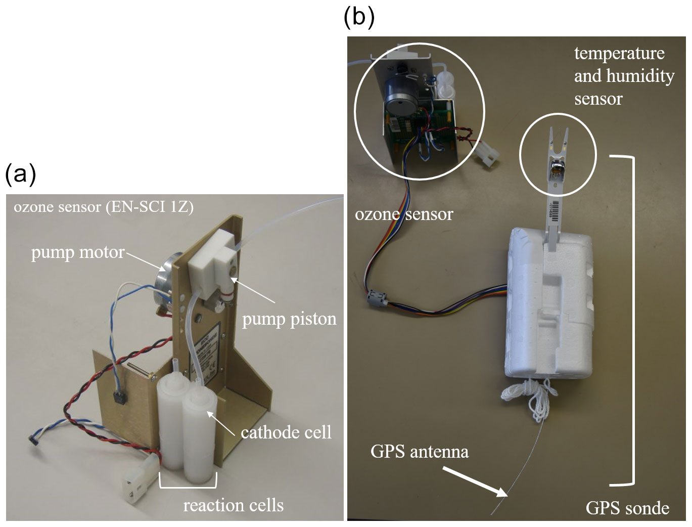
Figure 2 illustrates pump operation. First, ambient air taken into the pump is compressed until its pressure is balanced with the back-pressure associated with the hydraulic head pressure of the reaction cell (1). The compressed air is then discharged to the cell by the force of the piston (2). When the piston is completely pushed in, there is a dead space inside the pump (3), and the compressed air remaining in it expands until it is balanced with the ambient air pressure (4). The piston draws in a fresh sample of ambient air (5). The cycle is repeated for each pump rotation. The steady pump speeds typically range from 2400 to 2600 rotations per minute (RPM). Hydraulic head pressure, which is the main factor causing back-pressure, can be considered essentially uniform regardless of ambient air pressure, while the latter varies with altitude. Under these conditions, the air taken in is more compressed in step (1), and that in the dead space is more expanded in step (3). In other words, as ambient air pressure decreases, the volume of air intake (the pump flow rate) into the reaction cell also falls. Thus, the pump is affected by ambient air pressure, which governs its efficiency.

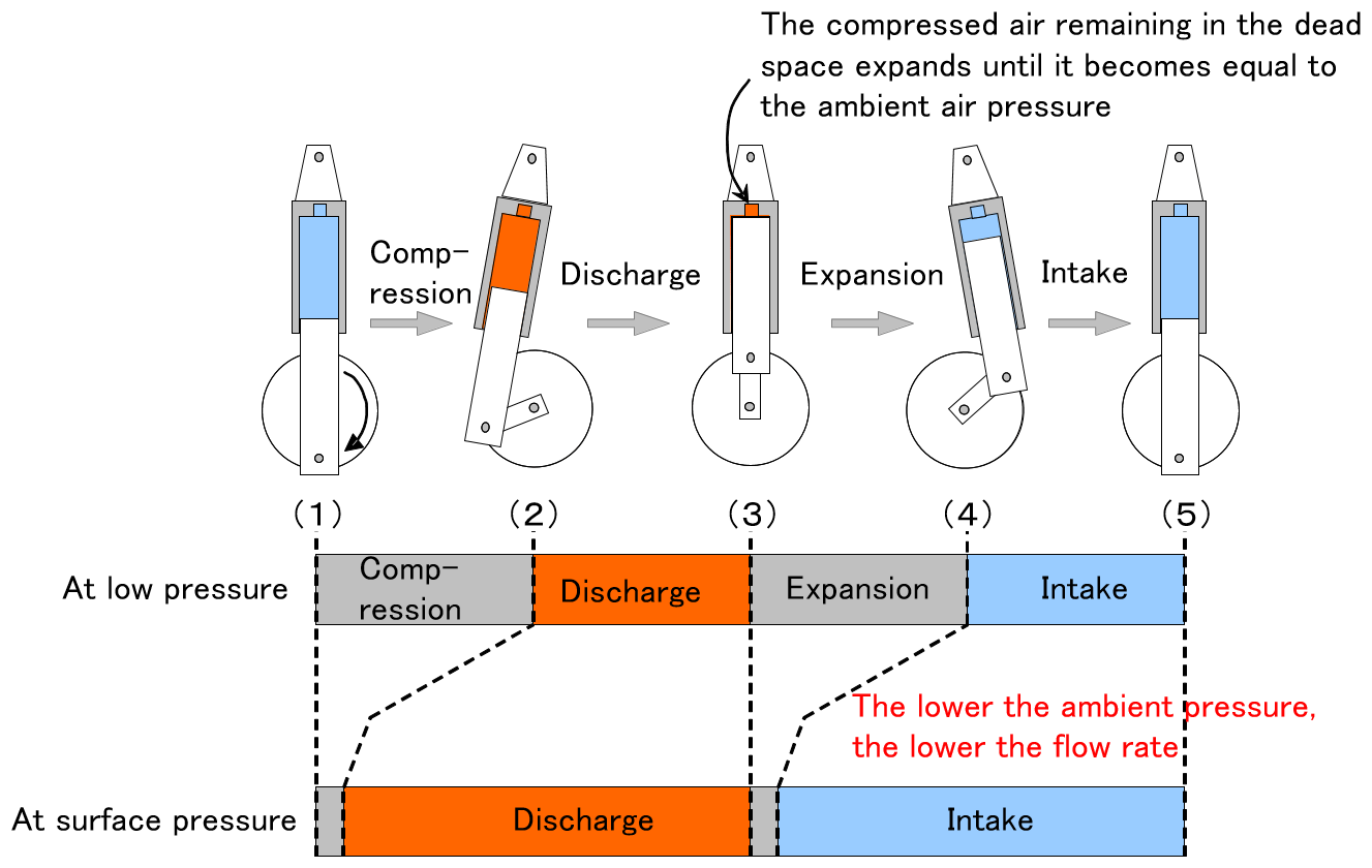
Figure 2 Piston pump operation during observation and the effect of dead space on pump efficiency.

Based on laboratory pump flow measurements (Komhyr et al., 1986, 1995; Johnson et al., 2002), Smit and the Panel for the ASOPOS (2014) and Smit et al. (2021) provided useful tables listing pump flow correction factors and pump flow efficiencies as a function of air pressure. These values are averaged from experiments at the time of ECC-ozonesonde development and values recommended by the manufacturer. Causes of pump flow reduction (dead volume in the pump piston, pump leakage, hydraulic head pressure of the reaction solution in the reaction cell, etc.) can vary considerably among individual ozonesondes. To eliminate such observational uncertainties, it is necessary to accurately determine the pump efficiency of individual ozonesondes in preflight preparation. However, such determination is not normal practice in ozonesonde launches, as it is considered technically difficult and time-consuming. As a result, most ozonesonde profiles are produced using average pump-efficiency curves.

Individual pump efficiencies have already been measured by other investigators. For example, the National Oceanic and Atmospheric Administration/Climate Monitoring and Diagnostics Laboratory (NOAA/CMDL) developed a bubble flowmeter involving the use of silicone oil (Johnson et al., 2002) and showed that the conventionally used standard pump-efficiency correction tables (Komhyr et al., 1986, 1995) were underestimated as compared to the pump-efficiency corrections of currently manufactured ECC ozonesondes. The University of Wyoming also measured individual pump efficiencies using an airbag evacuation-type flowmeter equipped with an airbag (Johnson et al., 2002). However, as no pump-efficiency measuring systems are currently commercially available, we developed such a system at the Aerological Observatory in Tateno, Japan. Examining various measurement methods led to the adoption of an airbag method approach for ease of control. The system was automated in order to obtain pump-efficiency measurements with uniform quality and has been installed at the Tateno, Sapporo, Naha, and Syowa stations in sequence since 2009. The pump efficiency of individual ozonesondes is operationally measured at these stations, which have produced a significant amount of data since installation.

In this paper, Sect. 2 outlines the automated pump-efficiency measuring system, Sect. 3 details the measurement method and procedures for the airbag-type system, Sect. 4 describes pump-efficiency calculation, and Sect. 5 covers statistical results for pump efficiency as obtained from operational observations for the current decade and the long-term stability of the pump measurement system.

2 System overview

The automated pump-efficiency measuring system is roughly divided into three parts: a control unit, a pressure control unit, and a flow measurement unit. Figure 3 outlines the system, and Fig. 4 shows its actual appearance. The control unit is designed for control of the whole system via a PC with a module that communicates directly with peripheral equipment. The pressure control unit consists of a vacuum pump, a vacuum controller, and a digital barometer. The flow measurement unit consists of an airbag-type flowmeter in a vacuum desiccator that allows various pressure conditions down to 3 hPa.

Figure 3 Automated pump-efficiency measurement system for ECC ozonesondes.

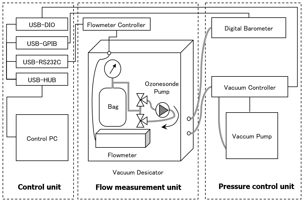
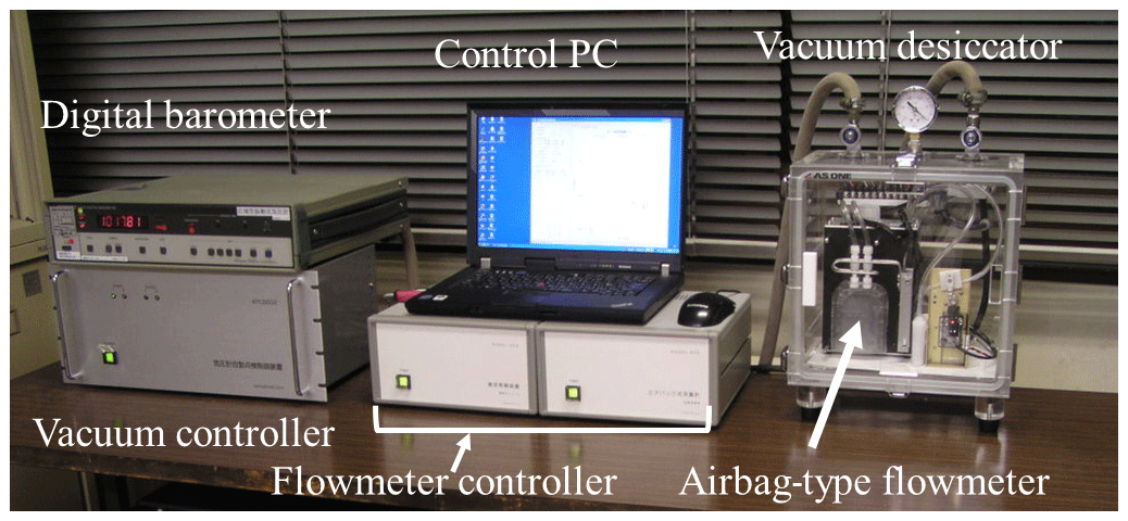
Figure 4 Actual appearance of the automated measurement system of the pump efficiency for the ECC ozonesonde.

The control unit consists of a Windows PC combined with various communication modules (DIO, GPIB, and RS232C) to control the entire system and collect measurement data. As these modules and the control PC are connected via USB, the system can be controlled using a general-purpose PC.

The Windows program used to adjust the pressure control unit and the flow measurement unit also enables conversion of various measurement data acquired from the flow measurement unit at regular intervals into physical values and collection of data together with other information such as digital barometer readings.

The pressure control unit controls air pressure in a vacuum desiccator to reproduce low-pressure environments. As ozonesondes are subjected to decreasing atmospheric pressure and low-temperature conditions (−60 to −80 ^∘C) during balloon ascent, initial efforts were made to reproduce both conditions. However, measurements for a low-temperature environment showed that temperature does not exhibit a linear relationship with pump efficiency and even shows a negligible effect, at least in the temperature range of actual atmospheric conditions. For this reason, pump efficiency was measured only with low-pressure environmental conditions. Since the minimum pressure of the unit is less than 3 hPa, the entire pressure range of ozonesonde measurements can be reproduced.

By manipulating the degree of exhaust valve opening in the vacuum controller with the control program, the speed of the vacuum pump (equal to the rate of decompression in the desiccator) can be adjusted. The pressurization rate can also be controlled by opening and closing the solenoid valve for atmospheric pressure release. With these adjustment functions, air pressure in the desiccator can be maintained to within approximately ±0.1 hPa of the target by setting the decompression rate to 0 during the flow measurement performed at each specified air pressure. At the start of depressurization and pressurization, a series of procedures is followed to prevent sudden air pressure changes in the desiccator, which might cause a backflow of oil from the vacuum pump to the desiccator. The control program allows safe execution of these steps.

The flow measurement unit consists of a vacuum desiccator, a flowmeter controller, and a control PC. Figure 5 shows the schematic diagram of the flow measurement unit.

Figure 5 Schematic diagram of the flow measurement unit.

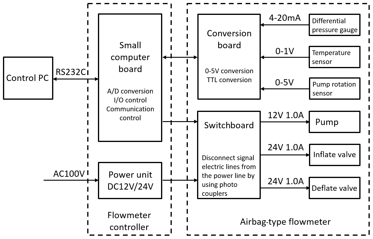
The ozonesonde pump and an airbag-type flowmeter are inside the vacuum desiccator. The flowmeter controller, which is set outside the vacuum desiccator, supplies power to the flowmeter, allows monitoring and control of status every millisecond using a built-in microcomputer (H8/3052F), and enables issuance/receipt of control commands and transfer of measurement data to the control PC using RS232C. This allows real-time measurement control on a millisecond scale, thereby significantly reducing the control PC's load.

The airbag-type flowmeter has a conversion board to adapt the output of various sensors to the input of a small computer board and a switchboard to control the power supply of the pump and the solenoid valve. The power supply/signal lines are electrically isolated using photo couplers to reduce noise contamination. Figure 6 shows the airbag-type flowmeter piping connection. The inflation and deflation valves are fluororesin three-way solenoid types, with NO (normally open) to COM (common) communication when not powered and NC (normally closed) to COM communication when powered, and are switched alternately to pump air into and out of the airbag.

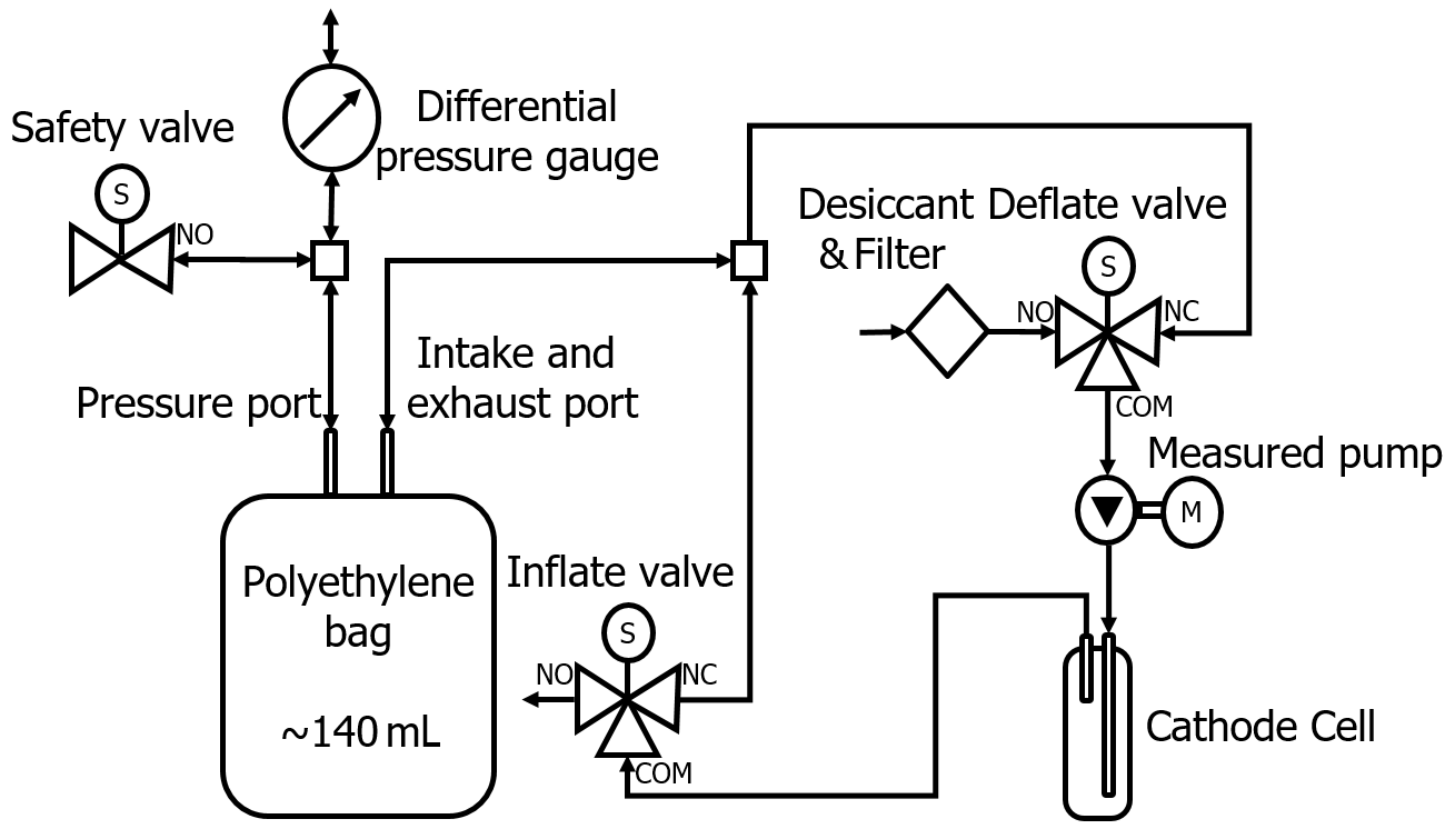
Figure 6 Airbag-type flowmeter piping connection. The 140 mL bag is made of polyethylene. The inflation and deflation of the bag are conducted by using two magnet valves. The pressure between the inside and outside of the bag is measured with a differential pressure gauge. Temperatures in the bag and pump are measured by thermometers. The revolving speed of the pump is measured by an optical instrument.

The airbag is equipped with a port for differential pressure measurement separately from the intake and exhaust ports to ensure stable differential pressure measurement. A model 265 Setra Systems pressure transducer is used as a micro-differential pressure gauge with a measurement range of ±1 hPa and an accuracy of ±1 % of full scale.

The airbag material must be able to deform with very weak forces, be airtight and have little stretch and shrinkage, and be easy to work with and manipulate. Among the available materials, polyethylene film with a thickness of 0.01 mm demonstrated optimal behavior. Since wrinkles caused by uneven deformation as the airbag repeatedly expands and contracts can cause erroneous measurements, a smaller fluoroplastic film is placed inside the bag. After repeated prototyping, an airbag with a shape similar to that of an intravenous drip bag was adopted.

The main control and measurement features of the flow measurement unit are as follows.

• Pump ON/OFF control

• Control of flowpath switching via an inflation/deflation valve

• Measurement of differential pressure inside/outside the airbag (0.01 hPa)

• Measurement of pump, desiccator, and airbag temperature (internal thermistor) (0.1 ^∘C)

• Measurement of pump motor speed with a handmade digital tachometer attached to the ozone sensor (0.1 RPM). The tachometer shines light on the rotating part of the pump and detects reflection to determine the number of revolutions. The rotating part is partially covered with a nonreflective black sticker to indicate a full revolution by the tachometer.

• Time interval measurement triggered by the specified differential pressure (1 ms)

3 Method for measuring pump efficiency using the airbag method

3.1 Concept

The concept of estimating the pump flow rate (pumping power) using an airbag involves timing inflation from the least to most inflated state and vice versa. The airbag internal volume V_airbag in its most inflated/deflated states is assumed to be constant, regardless of ambient pressure, as long as the internal pressure and external pressure are equal. The pump flow rate S(p) at a given pressure p can be estimated with the average inflation and deflation time t(p) as

$$\begin{array}{}\text{(1)}& S\left(p\right)=V_{\mathrm{airbag}}/t\left(p\right).\end{array}$$

Pump efficiency k(p) at the given pressure p, defined as the ratio of the pump flow rate to that estimated at ground-level pressure p₀, can be calculated as

$$\begin{array}{}\text{(2)}& \begin{array}{rl}k\left(p\right)& =S\left(p\right)/S\left(p_{\mathrm{0}}\right)\\ & =\left(V_{\mathrm{airbag}}/t\left(p\right)\right)/\left(V_{\mathrm{airbag}}/t\left(p\right)\right)\left(V_{\mathrm{airbag}}/t\left(p_{\mathrm{0}}\right)\right)\\ & =t\left(p_{\mathrm{0}}\right)/t\left(p\right).\end{array}\end{array}$$

As this equation shows, the exact volume of the airbag does not need to be known.

Meanwhile, it is necessary to assess whether the airbag is fully inflated or deflated, which is done by evaluating its internal/external differential pressure. The threshold was set to ±0.8 hPa (+: inflation; −: deflation), as discussed later. The flow was switched using two valves shown in Fig. 6 when the differential pressure reached the threshold. Figure 7 shows temporal variations in differential pressure from the time of maximum deflation. A series of measurements was made when the flow was switched at ground-level pressure. Plotting of differential pressure during deflation from around the time of maximum inflation (red line) shows that the inflation and deflation times are equal, since they match at the time of maximum deflation. In addition, since the pump flow rate at ground level was stable, the elapsed time can be considered associated with the internal volume of the airbag. These results indicate that differential pressure values during inflation and deflation all represent a certain airbag volume. From the above, pump efficiency can be determined from Eq. (2) by measuring the time interval at which a certain differential pressure is observed.

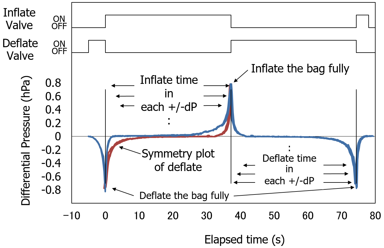
Figure 7 Schematics of pressure differences between the inside and outside of the bag as a function of lapsed time. The blue line plots four time-average difference-pressure values with bag inflation/deflation changed when the difference pressure reaches 0.8 hPa. The red line shows a symmetric reference of deflation to maximum inflation at an elapsed time of approximately 36 s. On/off lines for inflation and deflation are plotted at the top.

The pump correction factor (the reciprocal of the pump efficiency) is obtained only from the time required for airbag inflation and deflation, and in the case of differential pressure Δp is expressed from Eq. (2) as follows:

$$\begin{array}{}\text{(3)}& {\text{pcf}}_{\mathrm{0}}(p,\mathrm{\Delta }p)={\displaystyle \frac{\mathrm{1}}{k\left(p\right)}}={\displaystyle \frac{t(p,\mathrm{\Delta }p)}{t(p_{\mathrm{0}},\mathrm{\Delta }p)}},\end{array}$$

where pcf₀(p,Δp) is the pump correction factor for differential pressure Δp at air pressure p and t(p,Δp) is the time taken to reach Δp at p (p₀ is ground-level pressure). In practice, however, the effects of differences in differential pressure thresholds and temperature changes due to heat generated by solenoid valves and pump motors can cause measurement errors, giving rise to a need for consideration of a correction method. The details are described in Sect. 4.

3.2 Measurement sequence and measured value

In the series of measurements, the automated pump-efficiency measuring system recorded values at ground-level pressure (six times) and at 500, 200, 100, 50, 30, 20, 10, 7, 5, 4, and 3 hPa (four times each). In each case, as the first record was at the “break-in” of the airbag, values from the second time onward were taken as the actual measurements. The final pump correction factor was the average of values observed at the time of inflation and deflation. For each measurement, the system also acquired additional data on the time taken for the bag's internal/external differential pressure to reach ± 0.1, 0.2, 0.3, 0.4, 0.5, 0.6, 0.7, and 0.8 hPa (+: inflation; −: deflation), pump temperature, and bag internal temperature. After the cycle of measurements at the different pressure levels, six measurements at ground pressure were made to check the reproducibility of pump operation. The measurement pressure, the number of measurements, the differential pressure threshold, and other settings for the sequence can be changed in the control program.

3.3 Consideration of the back-pressure (load) effect

The ECC ozonesonde has a Teflon rod protruding from the bottom of the reaction cathode cell, allowing the tube from the pump to be guided appropriately into the reaction solution by sliding it over the rod, which narrows air flow and produces pressure resistance. Additionally, in actual ozonesonde observation, reaction cells are filled with a solution. As back-pressure necessarily affects pump efficiency with these conditions, the back-pressure effects of the Teflon rod and the reaction solution on pump efficiency were examined. In all measurement tests, the same ECC-type (EN-SCI 1Z) sensor was used. This section describes the outcomes.

Figure 8a shows the results of comparison between cases in which the pump is directly connected to the flowmeter from its exhaust port and in which air flows through an empty reaction cell. The experiment showed that pump efficiency decreased (by up to approximately −6 % at 3 hPa) with connection through the cell and that the cell itself generated back-pressure, possibly due to the presence of the Teflon rod.

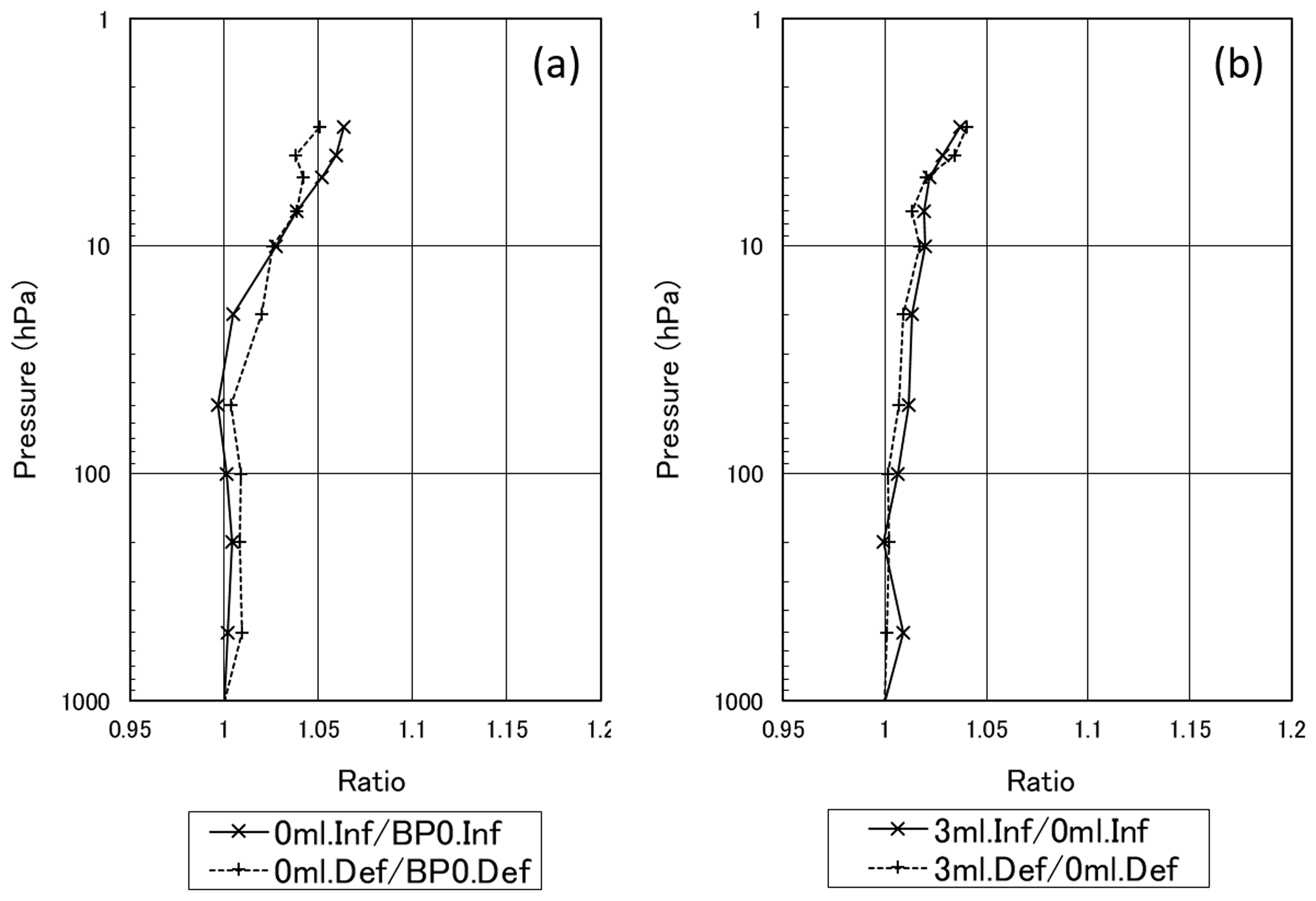
Figure 8 (a) Ratio of pump efficiency with a direct connection to the flowmeter from the pump exhaust port and through an empty reaction cell. (b) Ratio of pump efficiency between an empty reaction cell and one with the standard 3 mL of ECC silicon oil. Inf: inflation; Def: deflation; BP0: back-pressure 0 hPa; 0 mL: no reaction solution; 3 mL: 3 mL of reaction solution.

The relationship between the volume of the reaction solution and back-pressure was also examined. However, if pump efficiency is measured with an in-cell solution, the airbag-type flowmeter will fail due to backflow caused by boiling of the solution during flow observation, especially under low-pressure conditions. Accordingly, silicon oil with almost the same specific density as the reaction solution was used instead. Figure 8b shows the results of the comparison between an empty reaction cell and one with 3 mL of an ECC-type standard reaction solution, indicating that the load caused by the solution also reduced pump efficiency (by up to approximately −4 % at 3 hPa). The solution's head pressure is considered to have produced this effect.

The above outcomes indicate that a filled reaction cathode cell generates back-pressure, thereby affecting pump efficiency, as in real atmospheric conditions. The results in Fig. 9 show the correlation of back-pressure and solution volume in the cell at ground-level pressure. Back-pressure is approximately 3 hPa for the standard ECC-type reaction solution volume of 3 mL. To reproduce this load, the length and diameter of the piping were adjusted, and a load of 3 hPa was applied to the exhaust side with no solution in the cell. All further pump correction factors reported in Sects. 4 and 5 are always measured and determined with a 3 mL reaction solution in the cathode cell.

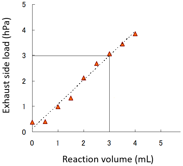
Figure 9 Exhaust-side load with a reaction cell; 3 mL of the standard reaction solution is equivalent to a load of approximately 3 hPa.

4 Pump correction factor calculation

As discussed above, a number of factors can cause observation errors in pump-efficiency measurements. This section outlines correction for such errors.

4.1 Correction for effects of in-pump heat generation

The study's series of pump-efficiency measurements began with ground-level pressure and continued with lower-pressure values. As the pump motor gradually heated up due to friction, the exhaled air was warmer in the later stages. Volume changes caused by the heating of inflowing air caused errors requiring correction in the results. As the heat capacity of air discharged from the pump is relatively small, it was assumed that air was warmed to the same temperature as the pump while passing through it, and the initial pump correction factor pcf₀(p,Δp) was adjusted as

$$\begin{array}{}\text{(4)}& {\text{pcf}}_{\mathrm{1}}(p,\mathrm{\Delta }p)={\text{pcf}}_{\mathrm{0}}(p,\mathrm{\Delta }p){\displaystyle \frac{T_{\mathrm{pump}}(p_{\mathrm{0}},\mathrm{\Delta }p=\mathrm{0.8})}{T_{\mathrm{pump}}(p,\mathrm{\Delta }p=\mathrm{0.8})}},\end{array}$$

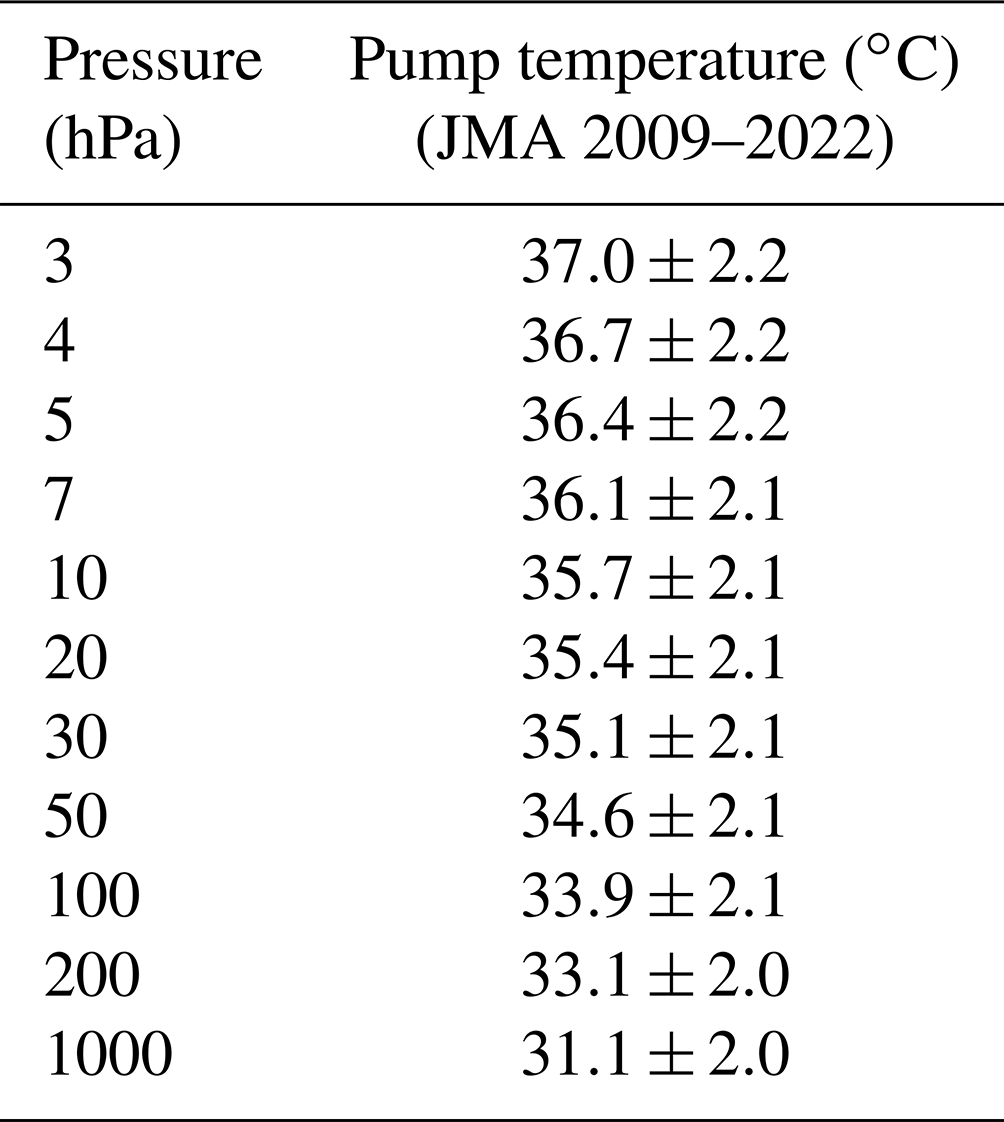
where T_pump(p,Δp) is the pump temperature (K) at differential pressure Δp with air pressure p (p₀ is ground-level pressure). These are temperature values at a differential pressure of 0.8 hPa (the most inflated state). Table 1 shows the average pump temperature during efficiency measurements performed by the JMA from 2009 to 2022. Measurements started after 30 min of warmup measurements, and the temperature typically increased by 5–6 ^∘C as the measurement progressed.

Table 1 Pump-temperature measurement results for Sapporo, Tateno, and Naha from 2009 to 2022.

4.2 Correction for differential pressure effects

The measurement time is defined as that required for the pump to exhaust all air and inflate the airbag from zero volume to V_airbag or to deflate it similarly under atmospheric pressure p. However, the airbag is actually further inflated or deflated in relation to the differential pressure ±Δp in addition to the ambient air pressure p. Differential pressure thus enables determination of bag content and internal volume. There is a need to consider related effects on the measurement time by converting the air pressure change inside the airbag into a volume change. Using the Boyle–Charles law (assuming no change in temperature), the internal volume of the airbag, V_airbag, changes with the ratio of the airbag differential pressure Δp to the ambient air pressure p. Accordingly, the measurement time t_m for the net measurement time t(p) at the air pressure p is expressed as

$$\begin{array}{}\text{(5)}& t_{\mathrm{m}}=t\left(p\right)\cdot \left(\mathrm{1}+\mathrm{\Delta }p/p\right).\end{array}$$

Here, it can be seen that lower ambient pressure p values produce a larger effect on the measurement time. To check the effects of this operation (referred to here as pressure correction) using t_m as the measurement time, the differential pressure threshold was varied from ±0.1 to ±0.8 hPa in turn, the pump efficiency with this correction was determined for each pressure, and comparison to values without correction was performed. Figure 10 shows the results of comparison at an ambient pressure of 3 hPa. It can be seen that pressure correction is generally effective, but the correlation between the pump correction factor and the differential pressure threshold remains high. The effects of differential pressure can therefore be seen as another pump loading factor. Thus, if differential pressure acts as an exhaust-side (intake) load when the airbag is inflated (deflated), the results can be seen as consistent with those of the previous pressure correction. However, deriving a correction for this effect is not straightforward, as loads change during measurement and each pump responds differently. Measurements at even lower differential pressure thresholds should be considered to avoid such effects, but there is a limit to the thresholds that can be set: very-low differential pressures are outside the detection limit of the micro-differential pressure gauge, and time-interval measurement is prone to errors. However, since the pump correction factor without differential pressure correction shows a very high correlation with the differential pressure threshold, the y intercept of the regression line can be comprehensively used as an estimate of the pump correction factor for a zero threshold. Accordingly, the pump correction factor corrected for the effects of differential pressure in actual measurement can be estimated from the regression line obtained from the time taken at each differential pressure threshold. The correction factor pcf₂(p) at zero differential pressure with this approach is

$$\begin{array}{}\text{(6)}& {\text{pcf}}_{\mathrm{2}}\left(p\right)={\text{pcf}}_{\mathrm{1}}\left(p,\mathrm{\Delta }p=\mathrm{0}\right).\end{array}$$

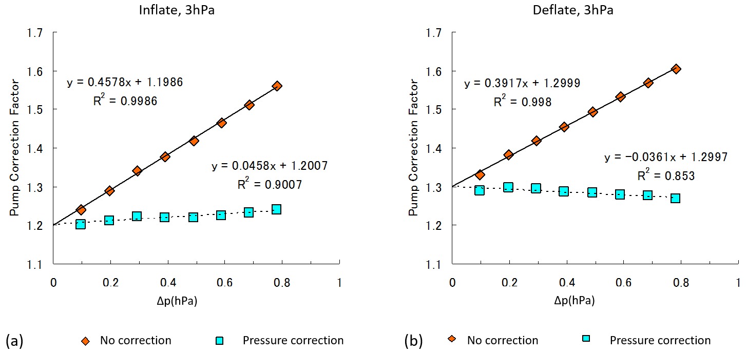
Figure 10 Pump correction factors calculated for various differential pressure thresholds. Values (representing the inverse of pump efficiency) are plotted with and without correction pressure correction. The values in panels (a) and (b) are based on the measurement times during expansion and contraction, respectively, at 3 hPa ambient air pressure, as determined with the pump's inlet and exhaust ports directly connected to a flowmeter.

4.3 Correction for temperature airbag capacity variations

As the polyethylene of the airbag used for differential pressure measurement expands and contracts with the temperature, changes in bag volume during measurement must be considered. Internal temperature gradually rises because the piping leading to the bag is heated by the solenoid valve and the circuit board inside the flowmeter housing, and the air pumped in is heated by pump friction. The temperature eventually rises by 5–6 ^∘C in a measurement sequence. Since related variations in airbag volume also cause measurement errors, pump efficiency is corrected using temperature data from thermistors near the bag.

After pump-efficiency measurement with airbag internal temperature variations in a thermostatic bath, it was found that approximately half of the temperature change rate affected the pump correction factor. We could confirm that Charles' law also holds when the pump temperature was changed using the same experimental apparatus. We postulate that this apparent inconsistency might be attributed to the effects of changes in airbag elongation and elasticity due to the thermal properties of the polyethylene film, offsetting the effects of volume change due to Charles' law by about half. The experimental results indicated that the pump correction factor after correction for temperature-dependent changes in airbag capacity can be expressed as

$$\begin{array}{}\text{(7)}& \begin{array}{rl}& {\text{pcf}}_{\mathrm{3}}\left(p\right)\\ & ={\text{pcf}}_{\mathrm{2}}\left(p\right)\left(\mathrm{1}-\mathrm{0.5}{\displaystyle \frac{T_{\mathrm{airbag}}(p_{\mathrm{0}},\mathrm{\Delta }p=\mathrm{0.8})-T_{\mathrm{airbag}}(p,\mathrm{\Delta }p=\mathrm{0.8})}{T_{\mathrm{airbag}}(p_{\mathrm{0}},\mathrm{\Delta }p=\mathrm{0.8})}}\right),\end{array}\end{array}$$

where T_airbag(p,Δp) is the airbag temperature (K) at differential pressure Δp with air pressure p (p₀ is ground-level pressure).

4.4 Application of pump-efficiency measurement results to ozone partial-pressure calculation

Pump efficiency k(p) at atmospheric pressure p is given by Kobayashi and Toyama (1966a) as

$$\begin{array}{}\text{(8)}& k\left(p\right)=\mathrm{1}-K\cdot \left({\displaystyle \frac{\mathrm{1}}{p}}-{\displaystyle \frac{\mathrm{1}}{p_{\mathrm{0}}}}\right),\end{array}$$

where p₀ is ground-level pressure (hPa) and K is a constant. According to Steinbrecht et al. (1998), when adiabatic change occurs in the pump, a power term (specific heat ratio γ≈1.4) should be added to the second term on the right:

$$\begin{array}{}\text{(9)}& k\left(p\right)=\mathrm{1}-K\cdot {\left({\displaystyle \frac{\mathrm{1}}{p}}-{\displaystyle \frac{\mathrm{1}}{p_{\mathrm{0}}}}\right)}^{\frac{\mathrm{1}}{\mathit{\gamma }}}.\end{array}$$

Assuming that this is actually a polytropic change related to the effects of heat exchange with the pump in addition to adiabatic change, the following approximate equation can be given:

$$\begin{array}{}\text{(10)}& \begin{array}{rl}\text{pcf}\left(p\right)& ={\displaystyle \frac{\mathrm{1}}{k\left(p\right)}}={\displaystyle \frac{\mathrm{1}}{\mathrm{1}-K\cdot {\left(\frac{\mathrm{1}}{p}-\frac{\mathrm{1}}{p_{\mathrm{0}}}\right)}^{\frac{\mathrm{1}}{n}}}}\\ & ={\displaystyle \frac{\mathrm{1}}{\mathrm{1}-c_{\mathrm{0}}{\left(\frac{\mathrm{1}}{p}-\frac{\mathrm{1}}{p_{\mathrm{0}}}\right)}^{c_{\mathrm{1}}}}},\end{array}\end{array}$$

where n is a polytropic index dependent on the ozone sensor, c₀ is a constant dependent on the ozone sensor, and c₁ is $\frac{\mathrm{1}}{n}$.

The application of pump-efficiency measurement results to ozonesonde observations is based on pcf₃(p), with the corrections described in Sect. 4.3. pcf₃(p) is calculated from the average of three measurements for each of inflation and deflation at a specified atmospheric pressure of 200 hPa or less. Using this equation, c₀ and c₁ in Eq. (10) are obtained by fitting. The pump correction factor pcf(p) at pressure p is then calculated from the same equation using the obtained constants c₀ and c₁. Ground pressure data are not used because pcf₃(p₀) should be 1.

5 Data from the JMA's automated pump-efficiency measuring system

Since 2009, the JMA has comprehensively evaluated EN-SCI ECC ozone sensor pump efficiency using the automated system, and pump correction factors calculated from the results are used to correct ozonesonde observations from Sapporo, Tateno, and Naha. This section presents the results of these measurements made over the last 13 years.

5.1 Comparison of pump correction factors between the JMA and other organizations

Figure 11 shows the results of pump correction factor measurements at Sapporo, Tateno, and Naha from 2009 to 2022 using sensors with similar serial numbers at each station. The values are generally consistent, with slightly larger differences at 3 hPa, where measurement accuracy is lower.

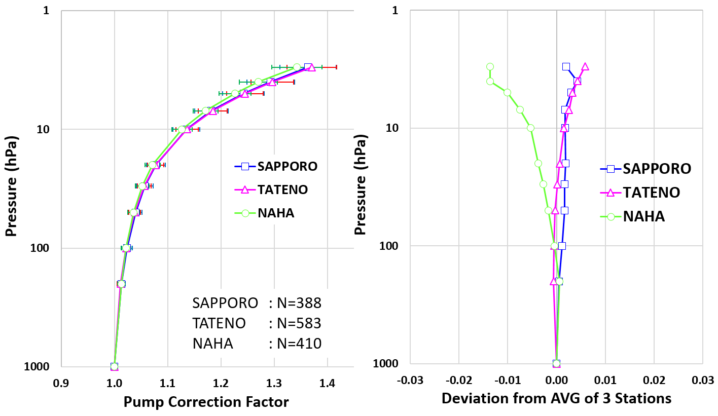
Figure 11 Pump-efficiency measurement for Sapporo and Naha from 2009 to 2018 and Tateno from 2009 to 2022. The error bars in the left-hand-side figure represent 1σ standard deviation. All the sites show close correspondence.

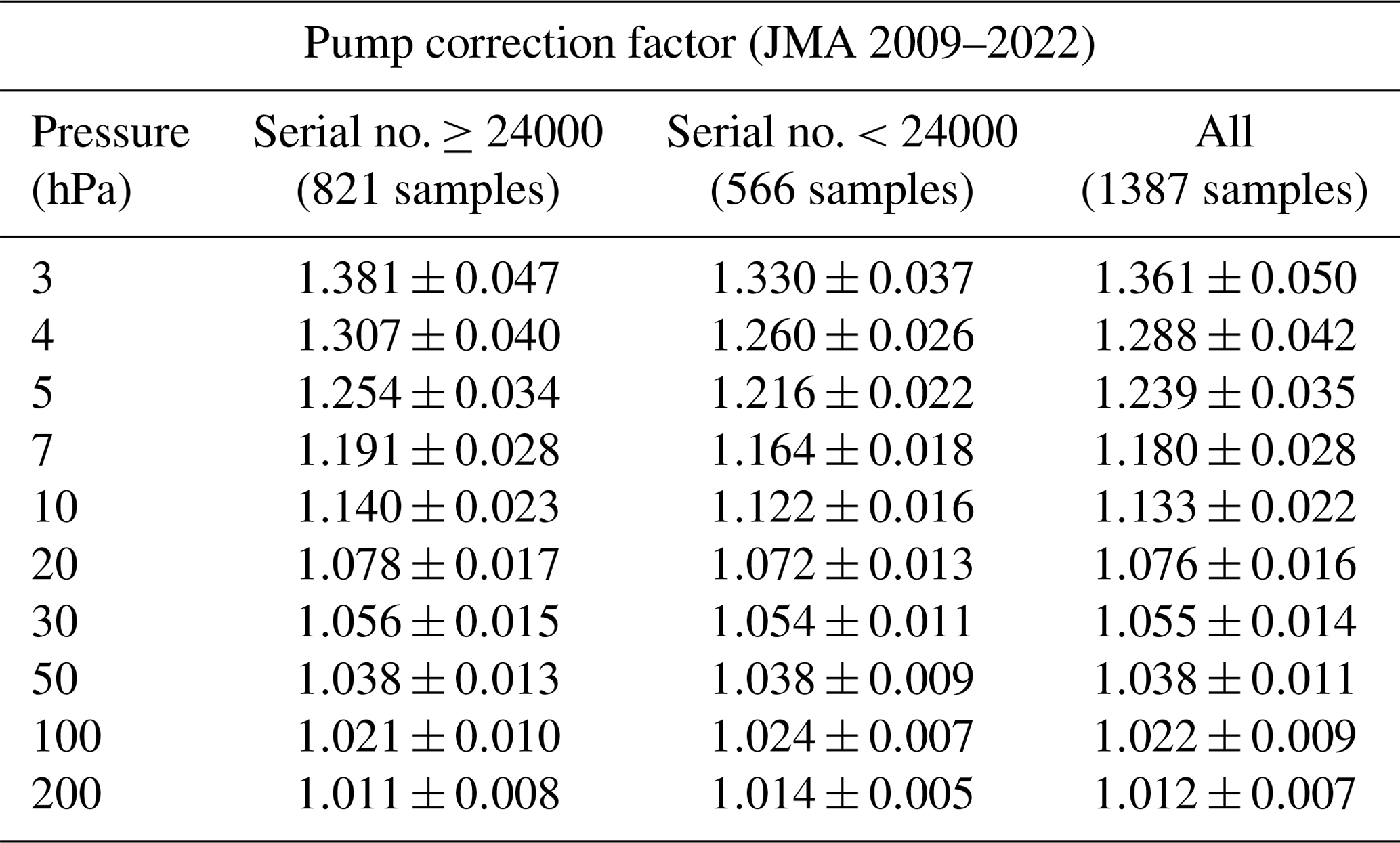
Figure 12 compares average pump correction factors for the same pump type (EN-SCI ECC) obtained by other organizations with typical JMA data. As will be illustrated in Sect. 5.3, Fig. 16, our measurements pointed to differences in the pump motor specifications of the ozonesondes delivered to the JMA before 2013 (serial numbers ≤24000) and after 2013 (serial numbers >24000). More specifically, the ozonesondes with serial numbers higher than 24000 turned out to have motor speeds that depend on the air pressure, and our measurements suggest that their motor speeds were unstable among production lots. The motor speed and its variability have an effect on the pump efficiency. Therefore, in Table 2, we also make a distinction between post-24000 and pre-24000 serial number samples for estimating the average JMA pump correction factors at the different pressure levels. It could thereby be noted that the average pump correction factors and their standard deviations are larger for post-24000 than pre-24000 serial numbers, at almost all pressure levels. For the comparison with the average pump correction factors measured by other organizations in Fig. 12, we nevertheless plotted the average JMA pump correction factors after serial numbers 24000, as these represent the most recent ozonesondes in use in the global network. Note that the average pump correction factors from the earlier studies in this figure are obtained from measurements with much lower ozonesonde serial numbers. Stauffer et al. (2020) also reported the discovery of an apparent instrument artifact that caused a dropoff in total ozone amounts from ozonesonde measurements at around one-third of global stations starting in 2014 to 2016, limiting suitability for ozone trend calculation. Stauffer et al. (2022) confirmed the presence of this dropoff in total column ozone at various EN-SCI ozonesonde sites around serial number 25250.

Measurements were conducted by the University of Wyoming with no exhaust-side loading using a reaction solution, and NOAA/CMDL made measurements with exhaust-side loading using non-evaporative oil instead of a reaction solution (Johnson et al., 2002). We replicated this work with longer tubing to simulate back-pressure from 3 mL of the reaction solution. Comparison indicated that pump correction factors for the period during expansion were close to those obtained by other organizations and that their dependence on ambient air pressure was also similar. These outcomes suggest the effectiveness of the proposed measurement system.

These measured pump flow efficiencies significantly differ from those reported by Komhyr et al. (1995) because, as noted by Smit et al. (2021), the values of Komhyr et al. (1995) represent overall correction including both pump flow efficiency and estimated stoichiometry increase over the period of flight.

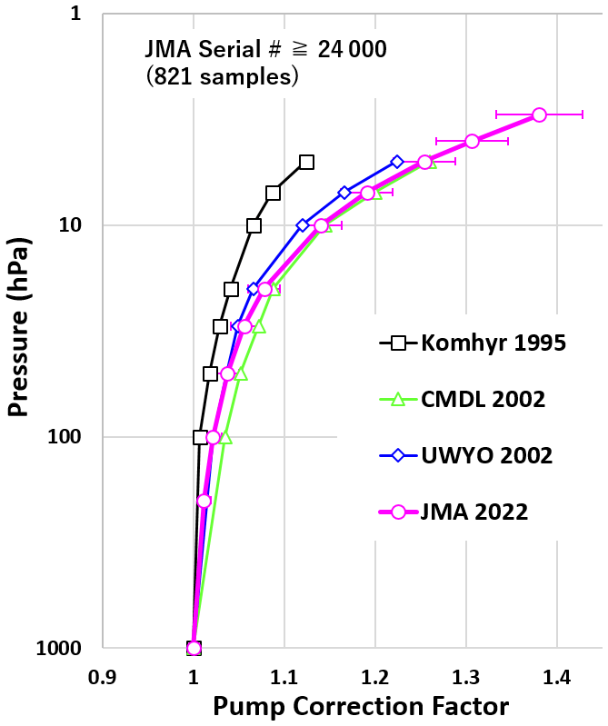
Figure 12 Comparison of pump correction factors from the JMA's airbag method with those from other experiments. Factors as a function of pressure are represented for the Komhyr et al. (1995) standard by the black line with squares, and JMA factors are represented by the pink line with circles. The error bars represent 1 SD. NOAA/CMDL average oil bubble flowmeter values are shown by the green line with triangles, and those from the University of Wyoming bag method are shown by the blue line with rhombuses (Johnson et al., 2002).

Table 2 Average JMA pump correction factors for pre- and post-24000 sensor serial numbers and for the entire time period (2009 to 2022).

5.2 Long-term system stability

The long-term stability of the measurement system was examined using sample data collected from four pumps at the Aerological Observatory in Tateno from 2010 to 2021. In addition to the correction outlined in Sect. 4, for this experiment only, the pump correction factors in the experiment were adjusted in line with pump motor speed to eliminate factor biases between different uses of the same pump using

$$\begin{array}{}\text{(11)}& {\text{pcf}}_{\mathrm{corr}}\left(p\right)=\text{pcf}\left(p\right){\displaystyle \frac{\text{MS}\left(p_{\mathrm{0}}\right)}{\text{MS}\left(p\right)}},\end{array}$$

where pcf_corr(p) is the pump correction factor after motor speed correction at atmospheric pressure p, pcf(p) is the same before correction, and MS(p) is the motor speed at p (p₀ is ground-level pressure). Figure 13 shows that flow correction factors for the four pumps exhibit no increasing or decreasing trends, although individual differences can be seen. This demonstrates the long-term stability of the measurement system and the absence of any aging degradation effect.

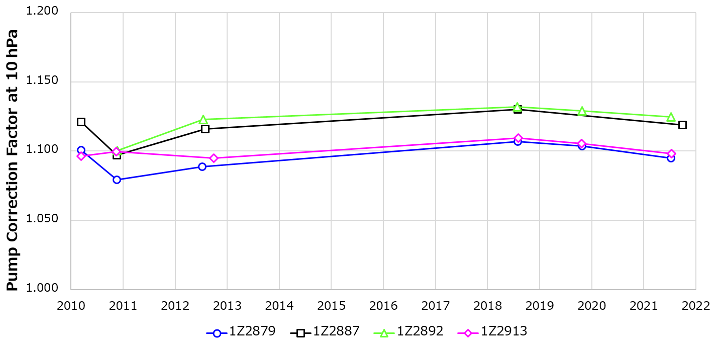
Figure 13 Pump correction factors at 10 hPa determined with the same four sensors from 2010 to 2021.

5.3 Decadal monitoring of individual pump efficiency

Figure 14 shows a time-series representation of individual pump correction factors at 50, 20, and 10 hPa as recorded at Sapporo, Tateno, and Naha from 2009 to 2022 (Sapporo and Naha terminated ozonesonde observations in February 2018). At all the stations, the pump correction factors exhibit temporal changes with a slightly increasing trend along different slopes. The slope is larger, with lower ambient pressure values around 2018 to 2019 (for 50 hPa: Sapporo: +1 % per 9 years; Tateno: +1 % per decade; Naha: +1 % or less per 9 years. For 20 hPa: Sapporo: +2 % per 9 years; Tateno: +2 % per decade; Naha: +2 % per 9 years. For 10 hPa: Sapporo: +4 % per 9 years; Tateno: +4 % per decade; Naha: +2 % per decade). The serial numbers of the ozone sensors used at each station were fairly balanced. As the pump-efficiency measurement system turned out to be very stable (Sect. 5.2), these pump correction factor trends should be ascribed to the ozonesonde pumps themselves.

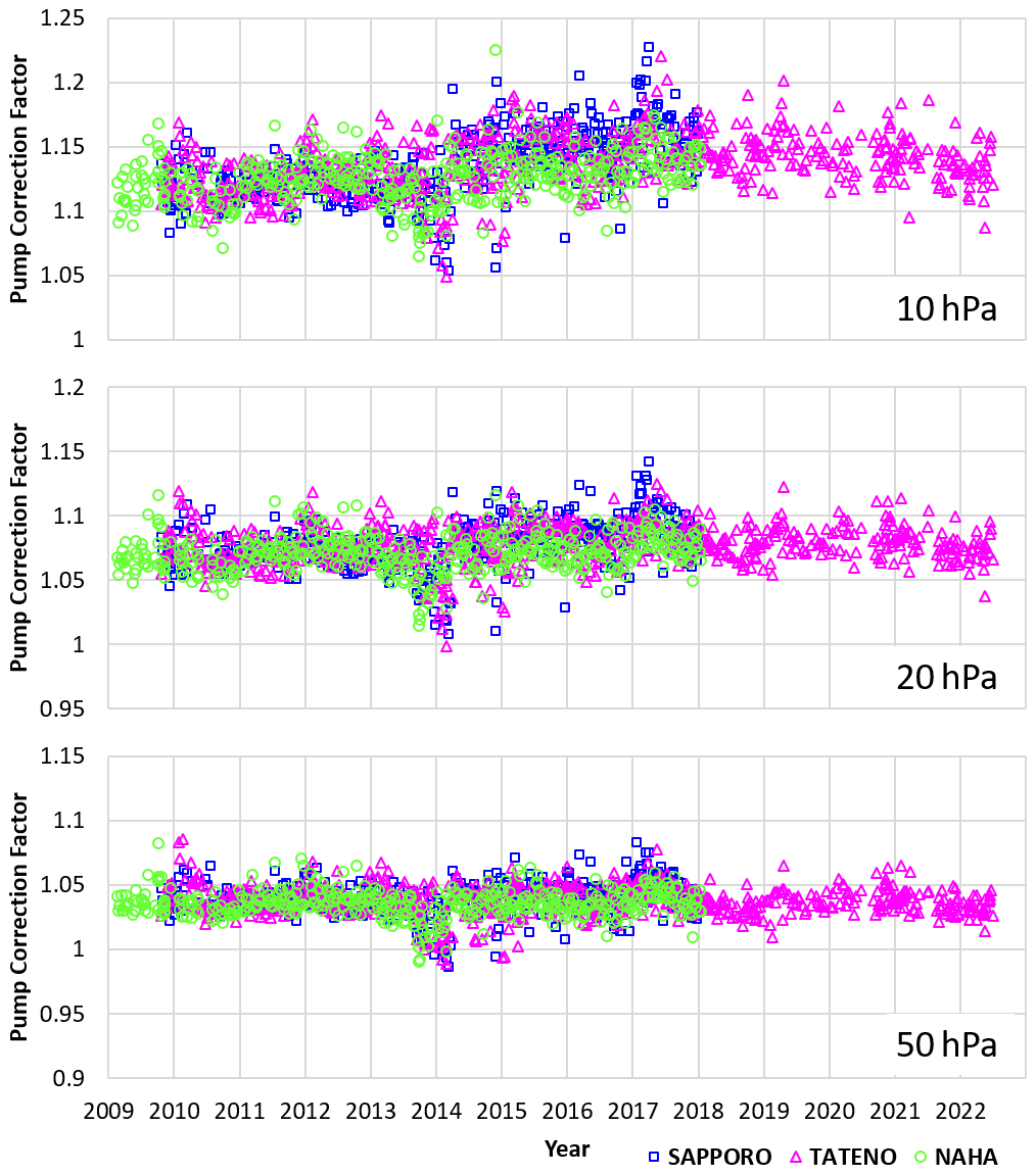
Figure 14 Pump correction factors for 2009 to 2022 (top to bottom: 10, 20, and 50 hPa). Over this 11-year period, the factor has changed by +1 % at 50 hPa, +2 % at 20 hPa, and +4 % at 10 hPa.

To investigate the extent to which this trend is caused by the pump, pump correction factors for the different stations are ordered left to right by serial numbers in Fig. 15a. The measurement numbers of the different stations are grouped together because the ozonesondes delivered to the JMA were divided into three by serial number and sent to each station. In Fig. 15b, the factors at 10 hPa are averaged for bins of 1000 serial numbers. It can be seen that the variability of the correction factors within each production lot is rather modest (1.8 %) and that differences between different production lots are mostly statistically insignificant.

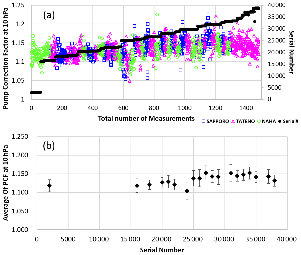
Figure 15 (a) Pump correction factors at 10 hPa from 2009 to 2022 sorted by ozone sensor serial number. (b) The same averaged for each bin of 1000 ozonesonde serial numbers for 2009 to 2022. Error bars represent standard deviation.

Figure 16 compares the mean measured values of the pump flow rate, motor speed, and pump stroke (i.e., obtained by dividing the flow rate by the motor speed) at ground-level pressure and at 10 hPa. Although there is no significant change in the measured flow rate, the pump motor speed increased by about 5 % to 10 %, and the pump stroke decreased by the same after serial number 24000. This indicates that a shortened pump stroke may increase the relative volumetric ratio of the pump dead space to the piston volume due to different motor specifications after serial number 24000 (Sect. 5.1), which may be a deteriorating factor in pump efficiency. Focusing on deviations between ground-level pressure and 10 hPa measurements, there is little change in motor speed differences but a visible trend in the pump flow rate and pump stroke differences. From this, it is considered that the difference in pump flow rate changes between the ground and lower-pressure values; that is, the difference in measurement time changes, resulting in an increased pump correction factor. In all the parameters, motor characteristics changed discontinuously on serial number 24000; after then, the standard deviations became larger, and the average values fluctuated with each group of sensor serial numbers. This is presumably because the motor pumps of post-24000 had a larger dependency on the air pressure, as mentioned in Sect. 5.1. Therefore, we consider the sample of serial numbers pre-24000 to be more reliable. Accordingly, the increasing trend of the pump correction factor is largely attributed to the ozonesonde side.

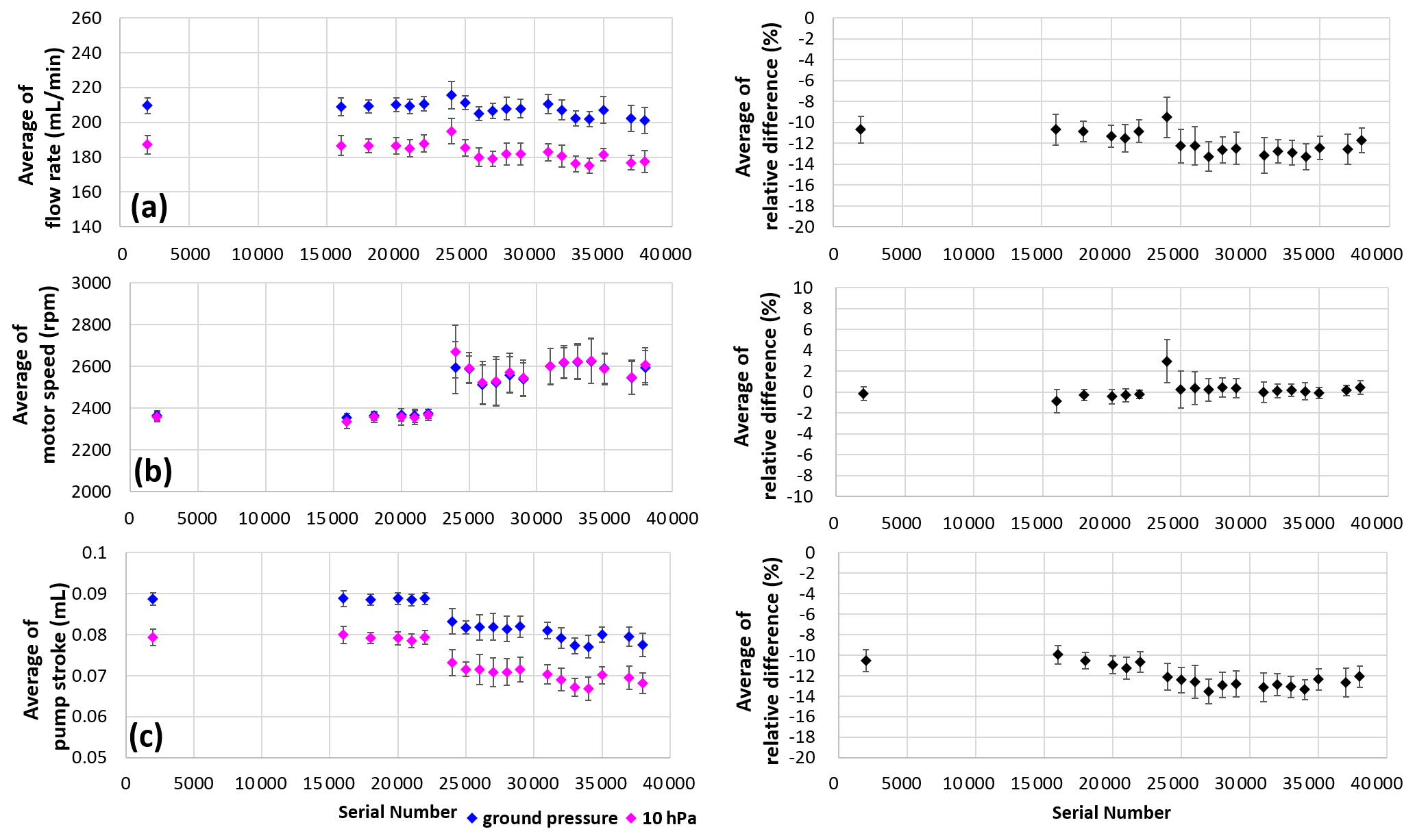
Figure 16 (a) Temporal variations in pump flow rate, (b) pump motor speed, and (c) pump stroke at ground pressure and 10 hPa averaged for each serial number of ozone sensors from 2009 to 2022 (left: measurement averages; right: relative difference from values at ground pressure).

5.4 Influence on the estimation of ozone concentration

This subsection discusses the effects of variability caused by changes in the characteristics of the pump flow rate outlined so far for total ozone. Figure 17 shows impacts on total ozone values if the table values of pump correction factors measured by the JMA for ozone sensor serial numbers post-24000 were used rather than measured individual pump correction factors. For each sounding, the relative differences between the total ozone calculated using the measured pump correction factors and that using the table values were determined during the period from 2009 to 2022. For calculation of the residual ozone column above balloon burst altitude, the mixing ratio was assumed to be equal to the measured value at the top of the sonde profile. The variation in total ozone was up to around 4 %. The standard deviation in the relative differences of total ozone values by lot was around 1 %, and that between production lots was around 0.6 %. As in Sect. 5.3, the pump correction factors tended to increase, but a decreasing tendency was seen with conversion to total ozone values. The step observed after 2014 is consistent with the dropoff in total ozone discussed by Stauffer et al. (2020, 2022).

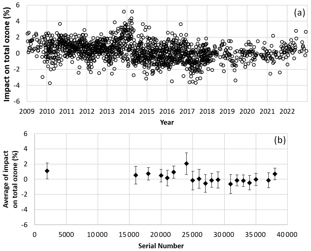
Figure 17 (a) Estimated impacts on total ozone values with use of the average pump-efficiency correction table. (b) Impacts on total ozone values for each serial number lot, with error bars indicating standard deviation.

6 Conclusion

The unique JMA system reported here enables fully automatic pump-efficiency measurement for individual ECC ozonesondes. Time-series representations of individual pump correction factors for EN-SCI ozonesondes calculated using this approach indicate temporal changes with an increasing tendency and variations depending on the production lot. These effects can be attributed to differences in the characteristics of mechanical pumps and pump motors for each production lot. In this situation, if a table of correction values for the pump flow-rate correction factor is used without individual pump-efficiency measurement, the total ozone value will be affected by up to around ±4  %.

Systematic biases in ozonesonde observations due to pump performance variations can lead to erroneous stratospheric vertical ozone trend values. To avoid the influence of lot-dependent pump correction factors in relation to EN-SCI's ozonesondes on stratospheric ozone trends and to enable accurate determination of actual atmospheric changes, it is advisable to determine the pump efficiency of each lot to pinpoint pump correction factor trends and enable adaptation to the calculation of ozone concentration. Although the costs of system production may hinder introduction at present, commercialization may enable the use of similar systems at lower cost in the near future.