the Creative Commons Attribution 4.0 License.
the Creative Commons Attribution 4.0 License.
 | 13 Jan 2023
Identifying optimal co-location calibration periods for low-cost sensors
Colby Buehler
Abhirup Datta
Drew R. Gentner
Kirsten Koehler
Low-cost sensors are often co-located with reference instruments to assess their performance and establish calibration equations, but limited discussion has focused on whether the duration of this calibration period can be optimized. We placed a multipollutant monitor that contained sensors that measured particulate matter smaller than 2.5 µm (PM2.5), carbon monoxide (CO), nitrogen dioxide (NO2), ozone (O3), and nitric oxide (NO) at a reference field site for 1 year. We developed calibration equations using randomly selected co-location subsets spanning 1 to 180 consecutive days out of the 1-year period and compared the potential root-mean-square error (RMSE) and Pearson correlation coefficient (r) values. The co-located calibration period required to obtain consistent results varied by sensor type, and several factors increased the co-location duration required for accurate calibration, including the response of a sensor to environmental factors, such as temperature or relative humidity (RH), or cross-sensitivities to other pollutants. Using measurements from Baltimore, MD, where a broad range of environmental conditions may be observed over a given year, we found diminishing improvements in the median RMSE for calibration periods longer than about 6 weeks for all the sensors. The best performing calibration periods were the ones that contained a range of environmental conditions similar to those encountered during the evaluation period (i.e., all other days of the year not used in the calibration). With optimal, varying conditions it was possible to obtain an accurate calibration in as little as 1 week for all sensors, suggesting that co-location can be minimized if the period is strategically selected and monitored so that the calibration period is representative of the desired measurement setting.
- Article
(880 KB) - Full-text XML
-
Supplement
(702 KB) - BibTeX
- EndNote


Instrument calibration is one of the main processes used to ensure instrument accuracy. In one method of calibration, measurements are compared between an uncalibrated instrument and a reference instrument, which can then be used to adjust the output of the uncalibrated instrument to see whether the data can meet performance standards (often in terms of accuracy and precision). In the case of low-cost air pollution sensors, the raw output is often a voltage or resistance instead of a concentration, so a calibration curve is needed to convert the raw output into practical units. Cross-sensitivities to environmental conditions or other pollutants, nonlinear responses, and variability between sensor units are common difficulties that must be considered when working with low-cost sensor data (Van Zoest et al., 2019; Levy Zamora, 2022; Li et al., 2021; Spinelle et al., 2015; Ripoll et al., 2019). Several methodologies have been used to derive the calibration equations needed to convert the raw data into useable concentrations, such as exposing the sensors to known concentrations in a laboratory setting and co-locating the sensors with a reference instrument, often in a similar setting to which the sensor is to be used (Taylor, 2016; Zimmerman et al., 2018; Mead et al., 2013; Ikram et al., 2012; Hagler et al., 2018; Cross et al., 2017; Holstius et al., 2014; Mukherjee et al., 2019; Gao et al., 2015; Heimann et al., 2015; Air Quality Sensor Performance Evaluation Center, 2016a, b, 2017; Levy Zamora et al., 2018a). Field co-location is a widely used calibration method, but a trade-off must be made between the time dedicated to collecting calibration data and the data collected at the final measurement location. There is currently no standardized co-location duration, and the reported co-location durations for low-cost sensors with reference instruments in recent work have varied from several days to several months (Mukherjee et al., 2019; Gao et al., 2015; Topalović et al., 2019; Kim et al., 2018; Spinelle et al., 2017; Pinto et al., 2014; Datta et al., 2020). To date, little discussion has focused on whether the selected periods were adequate for the deployment period or whether the calibration period can be optimized in future studies (Topalović et al., 2019; Okorn and Hannigan, 2021). In one study that assessed the impacts of the co-location duration for a low-cost sensor, Okorn and Hannigan (2021) randomly selected calibration periods of up to 6 weeks in duration from 6 weeks of methane data in Los Angeles. The calibration equations were then applied to data from an earlier month at the same location. They reported that longer calibration periods (i.e., 6 weeks) produced fits with a lower bias than fits from shorter calibration periods (i.e., 1 week). In that study, the 1-week calibrations yielded the best R2 values.
The central goal of this specific work was to identify the key factors that influence the duration of the co-location required to obtain sufficient data to achieve consistent calibrate curves for five low-cost sensors (particulate matter smaller than 2.5 µm, PM2.5; carbon monoxide, CO; ozone, O3; nitrogen dioxide, NO2; and nitrogen monoxide, NO) (Buehler et al., 2021). In addition, we aim to identify how this necessary calibration period can be optimized.
2.1 Data collection
Data collected at two sites were used in the co-location analyses based on the availability of reference instrumentation. The CO (Alphasense CO-A4), NO2 (Alphasense NO2-A43F), NO (Alphasense NO-A4), and O3 (MiCS-2614) sensors were co-located with reference instruments at the Maryland Department of the Environment (MDE) Essex site (ID 240053001) in Baltimore County, MD. The PM2.5 sensor (Plantower PMS A003) was concurrently co-located with a reference instrument at the MDE Oldtown site (ID 245100040) in Baltimore City, MD. The Essex site (lat 39.310833∘, long −76.474444∘) is about 11 km east of the Oldtown site (lat 39.298056∘, long −76.604722∘). Additional details about the sensors in the multipollutant monitor have been described in detail by Buehler et al. (2021) and Levy Zamora et al. (2022). Co-location data from 1 February 2019 to 1 February 2020 were used in the PM2.5 analysis, and co-location data from 1 February to 20 December 2019 were used in the CO, NO, NO2, and O3 sensor analyses. Due to an issue affecting the gas sensor inlet on the Essex monitor, the O3, NO2, and NO sensor data were unavailable after 20 December 2019. Hourly average data were used in all analyses. Both reference sites also measured hourly averaged temperature and relative humidity (RH). The ambient temperature and RH ranged between −11 and 36 ∘C and 14 % and 95 % over the full year, respectively. The temperatures and RHs measured inside the multipollutant pollutant monitors were slightly different from the ambient values due to direct sunlight warming the monitors and the small amount of heat produced by the sensors themselves within the box. The box temperatures and RHs ranged between −8 and 45 ∘C and 14 % and 80 %, respectively.
2.2 Assessing the role of co-location duration
We use different subsets of the full co-location period to create a suite of hypothetical co-location durations based on which the calibration models will be trained. For each hypothetical calibration co-location scenario (i.e., ranging from 1 to 180 consecutive days in 1 d increments), 250 sample calibration test periods were randomly selected of that duration. These test periods were used in the sensitivity analysis for each test condition to assess the range of potential resulting root-mean-square error (RMSE) and Pearson correlation coefficient (r) values. For example, a calibration duration of 1 d indicates that a 24 h period was randomly selected out of the available data, referred to as the “calibration period”, and the data from the 24 h were used to develop the calibration equations (see below) relating the raw sensor data to ambient conditions. This was then evaluated against all days not included in the calibration period, referred to as the “evaluation period”. The randomly chosen calibration periods could overlap, but no two periods were exactly the same. In Fig. S1 in the Supplement, the start times of 250 randomly selected PM2.5 calibrations are shown as an example. Each tested co-location duration produced 250 RMSE and r values, and only calibration periods with at least 70 % valid sensor and reference data were used in the analyses (e.g., a 24 h calibration period needed to have more than 16 h of valid data for both instruments). No laboratory or information from the manufacturer was used to additionally calibrate the sensors in this work. All data analysis was conducted using MATLAB (2020a).
Sensor data from the calibration period were used to determine the coefficients for multiple linear regression (MLR) models based on previously identified known environmental factors influencing concentration for each sensor (Levy Zamora, 2022). A generic MLR model is given by
where ReferencePollutant is the reference concentration at time t for a given pollutant, β0 is the constant intercept, β1 is the coefficient applied to the uncalibrated SensorPollutant value for a given pollutant at time t, and βn is the coefficient applied to Predictorn. Levy Zamora et al. (2022) have reported the predictors needed to calibrate these five low-cost sensors in detail. Briefly, the PM2.5 sensor model incorporated temperature and RH as predictors; the CO sensor model included temperature, RH, and time, where time refers to the current date and time that the data were collected; the NO2 sensor model included temperature, RH, NO, O3, and time; the O3 model included temperature, RH, NO2, and time; and the NO model included temperature and CO as predictors. The CO, O3, and NO2 sensors may exhibit baseline drift over the year, which is why the time predictors were included. The data used as the predictors came from the other sensors in the multipollutant monitor (e.g., the NO sensor model used the co-located low-cost CO sensor for the CO predictor). Once the regression coefficients were determined for a calibration period, this equation was applied to all data in the corresponding evaluation period.
For each calibration period tested, the RMSE and correlation coefficient values were determined by comparing the 1 h averaged reference and corrected sensor data from all hours during the evaluation period. The RMSE was calculated using Eq. (2), where Referencei and Predictedi are the corresponding ith 1 h averaged concentrations from the evaluation period with N data points.
An RMSE value of 0 would indicate a perfect agreement between the reference and the sensor. The correlation coefficient is a measure of the linear correlation between two data sets. It is a value between −1 and 1, where 1 indicates a strong positive relationship, −1 indicates a strong negative relationship, and 0 has no discernible relationship. The median RMSE and median r referenced in this paper refer to the median value from all 250 calibration scenarios for each duration. Outliers are defined as values that are more than 3 scaled median absolute deviations (MADs) away from the median.
We hypothesize that a user could strategically choose a co-location period to minimize the calibration period and that the co-location duration is not the only factor to consider when optimizing co-locating an instrument for calibration. In these analyses, we use the term “coverage” to indicate the representativeness of environmental conditions during a calibration period compared to that observed across the full data set (calibration and evaluation periods). In order to visualize how the environmental conditions during the calibration period compared to the evaluation period, we compared the range of temperature, RH, and other key pollutants from each period. For example, if the full RH ranged between 10 % and 90 % and the calibration period ranged between 20 % and 60 %, the RH coverage of that calibration period would be 50 % (40/80). Descriptive statistics of the reference data used in the calibration models from the full year are displayed in Table S1.
Table 1The median and range (1st–99th percentile) of the RMSE from 250 calibration runs from six co-location lengths (1 d, 1 week, 6 weeks, 1 month, 3 months, and 6 months) for five low-cost sensors. The median and range (min to max) of PM2.5, CO, NO2, O3, and NO reference concentrations were 7 (1–53) µg m−3, 199 (100–2950) ppb, 5.5 (1–58) ppb, 32 (1–110) ppb, and 0.5 (0.1–136.5) ppb, respectively.
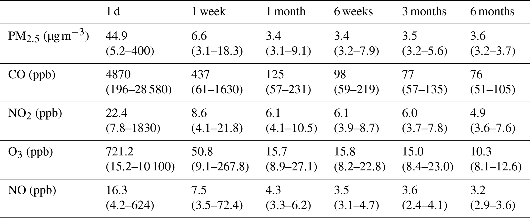

Figure 1The potential range of the (a, b) RMSE and (c, d) correlation coefficients (r) for a given co-location length for the low-cost PM2.5 and CO sensors. A calibration length of 1 d indicates that a random, continuous 24 h period was selected out of all available days. The RMSE for a given sample calibration was determined by comparing the 1 h averaged reference and corrected sensor data from the days during the evaluation period (i.e., all other days of the year not used in the calibration). For each calibration length tested, 250 sample calibration periods were used to assess the range of potential RMSE and correlation coefficient values. All sensors were calibrated using previously identified predictors in a multiple linear regression using data from the calibration period only. Reference PM2.5 concentrations ranged between 1 and 53 µg m−3, with a median concentration of 7 µg m−3, and reference CO concentrations ranged between 100 and 2947 ppb, with a median concentration of 199 ppb.
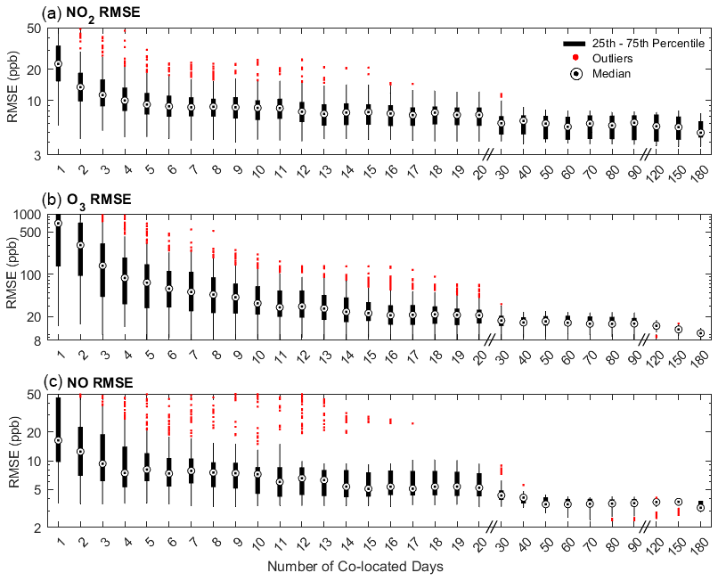
Figure 2The potential range of RMSE values for a given co-location length for three low-cost sensors (NO2, O3, and NO). A calibration length of 1 d indicates that a random 24 h period was selected out of all available days between February 2019 and February 2020. The RMSE for a given test calibration period was determined by comparing the 1 h averaged reference and the corrected sensor data associated with that calibration across the evaluation period (all days not included in the calibration period). For each calibration length, 250 randomly selected calibration periods were used to assess the potential RMSE range. All sensors were calibrated using previously identified predictors in a multiple linear regression using data from the calibration period only. The reference NO2 concentrations ranged between 1 and 58 ppb over the full year, with a median concentration of 5 ppb, the reference O3 concentrations ranged between 1 and 110 ppb, with a median concentration of 31 ppb, and the reference NO concentrations ranged between 0.1 and 137 ppb, with a median concentration of 0.5 ppb.
3.1 Impact of co-location duration on calibration performance
The range of RMSE values from 250 calibration periods in the sensitivity analysis of six co-location durations (i.e., 1 d, 1 week, 1 month, 6 weeks, 3 months, and 6 months) for all five low-cost sensors are shown in Table 1, and the box plots of the RMSE values from co-location durations ranging from 1 to 180 d are shown in Fig. 1 (PM2.5 and CO) and Fig. 2 (NO2, O3, and NO). Overall, longer calibrations resulted in lower median RMSE values. The greatest improvements in the median RMSE values were observed when increasing the co-location duration from 1 d to about 2 weeks. After about 6 weeks, diminishing improvements were observed in the median RMSE values for all the sensors except O3. The median RMSE for O3 decreased by about 5 ppb when increasing the duration from 6 weeks to 6 months. There was also a limited number of high outlier RMSE values for all of the sensors after about 2 months, indicating that most of the 250 calibrations were generally yielding similar RMSE values. In addition, the lowest RMSE values (e.g., 1st percentile) were similar for all co-location durations longer than about 1 week for many of the sensors. This suggests that optimized calibration periods can yield high-performance calibrations. For example, the RMSE values from the 1-week calibration periods for the PM2.5 sensor ranged between 3.1 and 18.3 µg m−3, and the 6-month calibrations ranged between 3.2 and 3.7 µg m−3. The 1st percentile RMSE values for the 1-week and 6-month calibration periods were also similar for CO (61 and 51 ppb, respectively), NO2 (4.1 and 3.6 ppb, respectively), O3 (9.1 and 8.1 ppb, respectively), and NO (3.3 and 2.9 ppb, respectively). The 10th percentile RMSE values were similar after about 1 month for most sensors. For example, the 10th percentile for PM was 3.4 at 1 month and 3.5 µg m−3 at 6 months (CO: 66 and 69 ppb, respectively; NO2: 4.3 and 4.1 ppb, respectively; O3: 11.0 and 8.4 ppb, respectively; NO: 3.5 and 2.9 ppb, respectively). The differences between the 1st and 99th percentile RMSE values for the 6-month scenarios were comparatively small for all sensors compared with the overall concentrations and ranges (e.g., the RMSE range at 6 months for PM2.5 was 0.5 µg m−3 compared with the annual average concentration of 8.3 µg m−3).
Table 2The median and range (1st–99th percentile) of correlation coefficients (r) from 250 calibration runs from six co-location lengths (1 d, 1 week, 1 month, 6 weeks, 3 months, and 6 months) for five low-cost sensors.
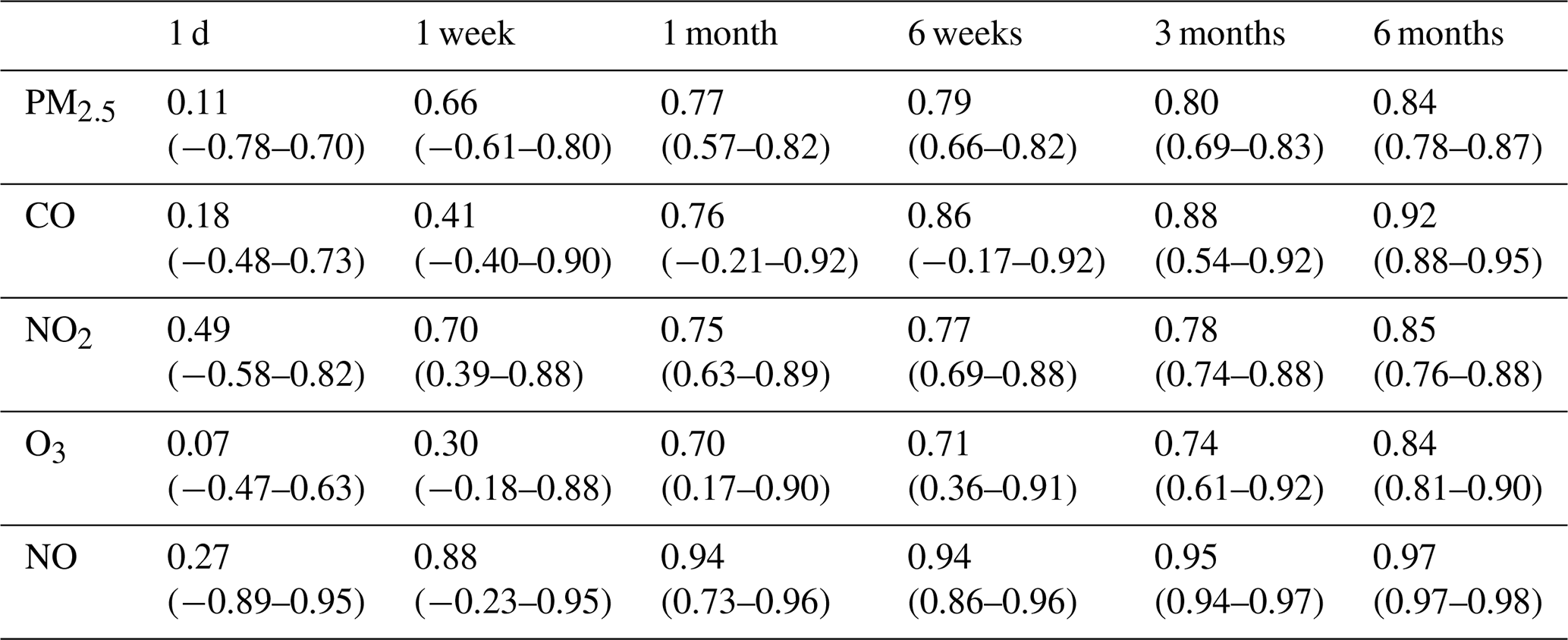
The ranges of correlation coefficients for the five low-cost sensors are shown in Table 2, and the box plots of the r values from co-location durations between 1 and 180 d are shown in Fig. 1 (PM2.5 and CO) and Fig. 2 (NO2, O3, and NO) in the Supplement. Overall, longer calibrations also resulted in higher r values, although it was possible to produce correlation coefficients at or above 0.6 in as little as 1 d for all five sensors in some individual test periods. After about 6 weeks, only incremental improvements were observed in the median correlations for all the sensors. For example, the greatest improvement in the median correlation after 6 weeks was observed for O3 which increased from 0.71 at 6 weeks to 0.84 at 6 months. All of the sensors were able to achieve reliably high correlations without poorly performing outlier cases (e.g., all 250 calibrations produced r > 0.6), but the co-location durations required to reduce this risk of outliers ranged between 18 d for the NO sensor and about 120 d for the CO sensor (Figs. S1 and S2).
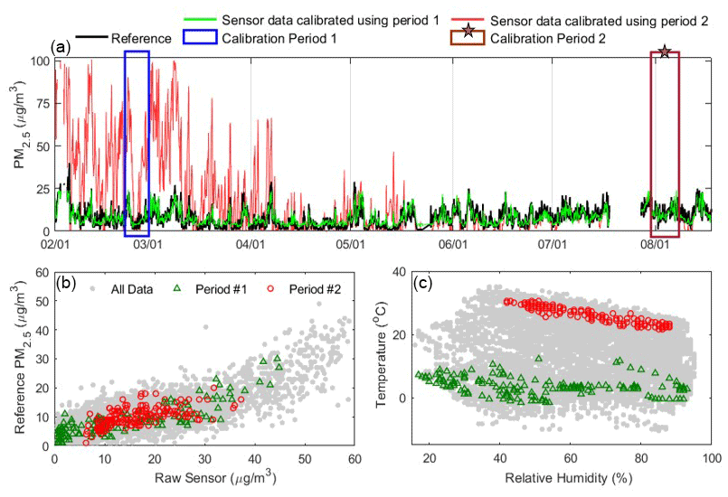
Figure 3Example comparison of two potential 1-week calibration periods. These were selected to illustrate the range of potential RMSE values that can result from using different periods of the same co-location duration. In the example here, “Calibration Period 1” yielded more accurate concentrations (shown in green; RMSE = 3.1 µg m−3), whereas “Calibration Period 2” performed poorly when considered across the whole evaluation period (shown in red; RMSE = 19.5 µg m−3). (a) The calibrated PM2.5 (µg m−3) time series are shown using the two test calibration periods and the reference data (black) from February to August 2019. (b) Scatterplot of PM2.5 data from the two calibration periods compared to reference data in comparison to the full data set. (c) Comparison of RH and ambient temperature for the two calibration periods compared to data from the full year.
3.2 Selecting optimal calibration conditions for co-location periods
The results show that the calibration performance from shorter-term co-locations varies considerably depending on the chosen co-location period. If a user wanted all 250 potential co-location periods for the PM2.5 sensor to have an RMSE below 4 µg m−3 and an r > 0.6, the minimum co-location duration that would ensure all calibration periods satisfied these two requirements would be 108 d at this site. However, 22 % of the 7 d co-locations also produced calibrations that satisfied these two requirements, so we analyzed the environmental factors during 1-week calibrations that led to low and high RMSE values. In Fig. 3 and Fig. S3, results from two 1-week calibration periods are shown to demonstrate the range of potential RMSE values for the PM2.5 sensor with differences in calibration conditions. The corresponding raw sensor, temperature, and RH data are also shown in Fig. 3b and c In this comparative example, “Calibration Period 1” produced more accurate concentrations during the evaluation periods (RMSE = 3.1 µg m−3), whereas “Calibration Period 2” performed poorly (RMSE = 19.5 µg m−3). Calibration Period 1 included a wider range of concentrations (1–45 µg m−3), temperatures (−2–12 ∘C), and RHs (17 %–93 %) and was able to yield similar concentrations to those produced using the reference data for the full year, whereas Calibration Period 2 was more limited in its range of conditions (6–37 µg m−3, 21–30 ∘C, and 42 %–88 %, respectively) and performed reasonably only during the summer months. In addition, the largest 6-month RMSE values (e.g., 3.7 µg m−3 for PM2.5 and 12.6 ppb for O3; Table 1) were generally comprised of more months during which ambient concentrations were low and less variable (summer and winter, respectively), and the scenarios with the lowest RMSE values included the months with the greatest concentrations observed in the data set. An analysis of the PM data in which the 250 randomly selected calibration periods were from between February 2019 and November 2019 and the evaluation period was held to between November 2019 and February 2020 (only one season) is shown in Fig. S4. The results are consistent with the original method.
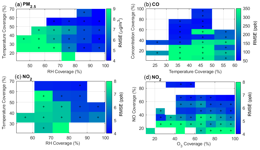
Figure 4Median RMSE values for PM2.5, CO, and NO2 sensors are shown as a function of data coverage (i.e., representation) of observed ambient conditions for key predictors within 1-week calibration periods. Bluer colors indicate better calibration results with lower RMSE values. The “+” markers indicate where there were at least 25 calibration runs that fell within that box. The “coverage” values indicate the representativeness of the 1-week calibration period compared to the full data set across all seasons. For example, if the temperature ranged from 0 to 40 ∘C over the full year and a given calibration period ranged from 0 to 12 ∘C, the temperature coverage of that calibration period would be 30 % (i.e., ). The ambient temperature and RH ranged between −11 and 36 ∘C and 14 % and 95 % over the full year, respectively.
Table 3Comparison of the median RMSE (µg m−3) for PM2.5 from 1-week calibration periods with different coverages of temperature and RH conditions. Only calibration periods with more than 50 % coverage of the PM2.5 concentration range were included in the table (> 50 % corresponds to 26 µg m−3 or more in this data set). For four scenarios (e.g., PM2.5 coverage > 50 %, RH coverage > 50 %, T coverage > 20 %), the 1st percentile RMSE, the 99th percentile RMSE, and the percentage of calibrations that exhibited all required conditions (e.g., RH > X % and T > X %) are shown (1st–99th percentile; %). For comparison, the median (1st–99th percentile) of the PM2.5 1-week calibration periods from the full data set (i.e., no coverage requirements) was 6.6 µg m−3 (3.1–18.3 µg m−3).

Based on these results, we hypothesized that a key element governing good calibration outcomes is if the calibration co-location period is representative of the evaluation period in terms of the required predictors in Eq. (1). Note that the required predictors are distinct for each sensor type, so optimal periods may differ by sensor. To evaluate this hypothesis, the median RMSE values for three sensors (PM2.5, NO2, and CO) were plotted as a function of the coverage of key predictors in the calibration period (Fig. 4). The gases NO2 and CO are shown because the NO2 sensor responds to numerous factors including other pollutants (i.e., cross-sensitivity) and the CO sensor exhibits a nonlinear response to temperature (Levy Zamora et al., 2022). The median RMSE of the corrected PM2.5 sensor is plotted as a function of RH and temperature coverage because they have been shown to drive biases in the PM2.5 sensor data (Sayahi et al., 2019; Levy Zamora et al., 2022, 2018a). If the coverage of key predictors is high, this indicates that the conditions during the calibration period are representative of the evaluation period (i.e., they cover a similar range of values). In general, the calibrations for PM2.5 become more accurate (lower RMSE values) as the RH coverage increases (i.e., moving to the right in Fig. 4a), and there is a slight improvement with increasing temperature coverage (i.e., Fig. 4a moving upwards). The lowest RMSE values were observed when the coverage was high for both temperature and RH. To further clarify the influence of coverage on calibration outcomes, the median RMSE values as a function of temperature and RH coverages when the PM2.5 concentration coverage was greater than 50 % are shown in Table 3. RH strongly influences the sensor's raw output, particularly compared with temperature (Levy Zamora et al., 2018b; Levy Zamora et al., 2022; Sayahi et al., 2019). To yield the best performing calibration outcomes, highly influential cross-sensitives or environmental factors (i.e., RH) should have a minimum coverage of about 70 % and secondary factors (i.e., temperature) should have a minimum coverage of about 50 %.
The NO2 sensor exhibits cross-sensitivities to O3 and NO in addition to responding to temperature and RH (Li et al., 2021; Levy Zamora et al., 2022), so an adequate calibration period should cover an adequate range for all four parameters. The reference NO2 concentrations ranged between 1 and 58 ppb, with a median concentration of 5 ppb. In general, the RMSE values in the NO2 plots decrease as the RH (Fig. 4c x axis), temperature (Fig. 4c y axis), and O3 coverage increase (Fig. 4d x axis), but the gradient is more clearly seen in the NO coverage (i.e., moving upwards on the y axis in Fig. 4d). The O3 sensor is an example of another sensor that exhibits a cross-sensitivity to another common pollutant (NO2; not shown in the main text), which has been demonstrated in a previous work (Levy Zamora et al., 2022). Additional examples of coverage of key variables for all the sensors are shown in Fig. S5.
For all three sensors in Fig. 4, the RMSE values decreased as the concentration coverage increased, but it was particularly notable for the CO sensor, likely due to the significant differences in seasonal concentrations (e.g., the peak reference CO concentrations from December and July were 2950 and 773 ppb, respectively). The reference CO concentrations ranged between 100 and 2950 ppb during the full year, with a median concentration of 199 ppb. This indicates that a period with only low concentrations may not be able to yield as accurate calibration curves if the evaluation period has a much broader concentration range than observed during the calibration period. In the CO sensor panel (Fig. 4b), greater temperature coverage generally resulted in lower RMSE values, but a key factor for the CO sensor is that the calibration must cover warm temperatures if the calibration is going to be applied to warm seasons. This is due to the notably different responses to high and low temperatures. This CO sensor exhibits minimal temperature effects below about 15 ∘C but strongly responds to warmer temperatures (i.e., the sensor will overestimate concentrations at higher temperatures if not properly calibrated) (Levy Zamora et al., 2022). More specifically, if a calibration period only included temperatures below 15 ∘C, those data could not reasonably be extrapolated to a warmer period because they would not be able to correct for this overestimation at high temperatures. Sensors with more linear responses are less sensitive to this issue because a smaller range may be more accurately extrapolated. We note that the NO and O3 sensors also exhibit nonlinear responses to temperature.
It is important to mention that Baltimore, MD, is a region that experiences a broad range of meteorological conditions each year, so the co-location duration must be long enough to capture an adequate range of conditions to fully characterize the calibration curves. The pollutants also exhibit significant seasonal variation at this location. In other regions where the weather conditions are less variable, shorter co-location durations may be more likely to produce accurate results. This is the primary reason why employing a “coverage” approach might be a more useful approach for identifying appropriate co-location durations. Moreover, we applied the calibration equations on data from a full year, but shorter co-location durations would likely be satisfactory if the calibration and measurement period were going to be completed under similar conditions (e.g., within one season). For example, if we limited the calibration and evaluation periods to between 1 June and 31 August 2019 (peak PM2.5 = 25 µg m−3), 70 % of 1-week co-locations would have an RMSE below 4 µg m−3 and an r > 0.6. Similarly, if we limited the calibration and evaluation periods to between 1 November 2019 and 1 February 2020 (peak PM2.5 = 53 µg m−3), 40 % of 1-week co-locations would have fulfilled these two requirements. Another benefit of strategically identifying co-location needs is that it may permit users of sensor networks to co-locate each device in the network for shorter periods to get device-specific calibration equations. By ensuring a minimum coverage of key factors for each device co-location period, calibration data between units would likely be more consistent, even if the data were collected from different periods. This would be particularly advantageous for sensor types that exhibit notable variability between units.
If little information is known about key predictors at the measurement sites, which is likely at remote locations, it may be possible to use historical meteorological data and general information about pollutant patterns (e.g., emissions and seasonal concentration patterns) to determine a representative range of conditions. Future work should explore whether a combination of multiple, shorter calibration periods in different seasons may produce reasonable calibrations for year-round data sets. However, in all cases, it is advisable to increase the estimated co-location periods in case of data loss or unusual air quality events to increase the probability of well-performing calibrations.
In this study, we assessed five pairs of co-located reference and low-cost sensor data sets (PM2.5, O3, NO2, NO, and CO) to identify key factors that influence the duration required to calibrate low-cost sensors via co-location. We compared the RMSE and correlation coefficient values from co-location periods spanning from 1 to 180 d. While longer co-location periods of up to several months generally improved the performance of the sensor, optimal calibration could be produced from shorter co-location lengths if the calibration period covered the span of conditions likely to be encountered during the evaluation period. We determined that many factors could increase the duration of co-location required, including if a sensor responds to environmental factors, such as temperature or RH; if the sensor exhibits a cross-sensitivity to another pollutant; if a response is nonlinear to any of these factors; and the duration of the full deployment (i.e., within a season or spanning multiple seasons). Particular attention must be given to sensors that exhibit a nonlinear response if the actual measurement period (e.g., the evaluation period) is going to extend into another season. These results suggest that co-location time can be minimized if selected strategically based on the typical characteristics of a region. The factors that strongly influence the sensor response should have a minimum coverage of about 70 %, and secondary factors should have a minimum coverage of about 50 %. Future work should evaluate if employing methods that account for the nonlinear responses of key predictors can further optimize the calibration of low-cost sensors as well as if more sophisticated comparisons of the statistical distributions of predictors across calibration periods are beneficial.
The data shown in the paper are available upon request from the corresponding author.
Additional figures shown in the Supplement include (1) the start times of 250 randomly selected PM2.5 calibration scenarios, (2) the potential range of Pearson correlation coefficients (r) for three low-cost sensors (NO2, O3, and NO) by co-location length, (3) a zoomed-in comparison of the two potential 1-week calibration periods corresponding to Fig. 3, (4) an analysis of the PM data in which the 250 randomly selected calibration periods were from between February 2019 and November 2019 and the evaluation period was between November 2019 and February 2020 for all of the considered calibrations, and (5) additional examples of coverage of key variables for all the sensors. Descriptive statistics of the reference data are shown in Table S1, and the median and range (1st–99th percentile) of the normalized RMSE values for six co-location lengths are shown in Table S2. The supplement related to this article is available online at: https://doi.org/10.5194/amt-16-169-2023-supplement.
MLZ and KK conceived of the presented idea. MLZ performed the calculations and created the visualization. All authors participated in designing and deploying instruments for data collection; optimizing the analytical approach; analysis and discussion of results; and contributing to writing the final manuscript.
The contact author has declared that none of the authors has any competing interests.
Publisher's note: Copernicus Publications remains neutral with regard to jurisdictional claims in published maps and institutional affiliations.
This publication was developed under Assistance Agreement No. RD835871 awarded by the U.S. Environmental Protection Agency (EPA) to Yale University. It has not been formally reviewed by the EPA. The views expressed in this document are solely those of the authors and do not necessarily reflect those of the Agency. The EPA does not endorse any products or commercial services mentioned in this publication. The authors thank the Maryland Department of the Environment Air and Radiation Management Administration for allowing us to co-locate our sensors with their instruments at the Baltimore sites. Misti Levy Zamora is supported by the National Institute of Environmental Health Sciences of the National Institutes of Health (award nos. K99ES029116 and R00ES029116). The content is solely the responsibility of the authors and does not necessarily represent the official views of the National Institutes of Health. Drew R. Gentner has had externally funded projects on low-cost air quality monitoring technology (EPA, HKF Technology), where the developed technology has been licensed by Yale to HKF Technology. Abhirup Datta is supported by the National Science Foundation (grant no. DMS-1915803) and the National Institute of Environmental Health Sciences (NIEHS; grant no. R01ES033739). Colby Buehler is supported by the National Science Foundation Graduate Research Fellowship Program (grant no. DGE1752134). Any opinions, findings, conclusions, or recommendations expressed in this material are those of the author(s) and do not necessarily reflect the views of the National Science Foundation.
This research has been supported by the Environmental Protection Agency (grant no. RD835871), the National Institute of Environmental Health Sciences (grant nos. K99ES029116, R00ES029116, and R01ES033739), and the National Science Foundation (grant nos. DMS-1915803 and DGE1752134).
This paper was edited by Maria Dolores Andrés Hernández and reviewed by Sreekanth Vakacherla and one anonymous referee.
Air Quality Sensor Performance Evaluation Center (AQ-SPEC): Field Evaluation of AirThinx IAQ, 2016, Field Evaluation of AirThinx IAQ, http://www.aqmd.gov/docs/default-source/aq-spec/field-evaluations/airthinx-iaq--field-evaluation.pdf?sfvrsn=18, (last access: March 2022), 2016a.
Air Quality Sensor Performance Evaluation Center (AQ-SPEC): Field Evaluation Purple Air (PA-II) PM Sensor, http://www.aqmd.gov/docs/default-source/aq-spec/field-evaluations/purple-air-pa-ii---field-evaluation.pdf?sfvrsn=2, (last access: March 2022), 2016b.
Buehler, C., Xiong, F., Zamora, M. L., Skog, K. M., Kohrman-Glaser, J., Colton, S., McNamara, M., Ryan, K., Redlich, C., Bartos, M., Wong, B., Kerkez, B., Koehler, K., and Gentner, D. R.: Stationary and portable multipollutant monitors for high-spatiotemporal-resolution air quality studies including online calibration, Atmos. Meas. Tech., 14, 995–1013, https://doi.org/10.5194/amt-14-995-2021, 2021.
Cross, E. S., Williams, L. R., Lewis, D. K., Magoon, G. R., Onasch, T. B., Kaminsky, M. L., Worsnop, D. R., and Jayne, J. T.: Use of electrochemical sensors for measurement of air pollution: correcting interference response and validating measurements, Atmos. Meas. Tech., 10, 3575–3588, https://doi.org/10.5194/amt-10-3575-2017, 2017.
Datta, A., Saha, A., Zamora, M. L., Buehler, C., Hao, L., Xiong, F., Gentner, D. R., and Koehler, K.: Statistical field calibration of a low-cost PM2.5 monitoring network in Baltimore, Atmos. Environ., 242, 117761, https://doi.org/10.1016/j.atmosenv.2020.117761, 2020.
Gao, M., Cao, J., and Seto, E.: A distributed network of low-cost continuous reading sensors to measure spatiotemporal variations of PM2.5 in Xi'an, China, Environ. Pollut., 199, 56–65, 2015.
Hagler, G. S., Williams, R., Papapostolou, V., and Polidori, A.: Air Quality Sensors and Data Adjustment Algorithms: When Is It No Longer a Measurement?, Environ. Sci. Technol., 52, 5530–5531, https://doi.org/10.1021/acs.est.8b01826, 2018.
Heimann, I., Bright, V., McLeod, M., Mead, M., Popoola, O., Stewart, G., and Jones, R.: Source attribution of air pollution by spatial scale separation using high spatial density networks of low cost air quality sensors, Atmos. Environ., 113, 10–19, 2015.
Holstius, D. M., Pillarisetti, A., Smith, K. R., and Seto, E.: Field calibrations of a low-cost aerosol sensor at a regulatory monitoring site in California, Atmos. Meas. Tech., 7, 1121–1131, https://doi.org/10.5194/amt-7-1121-2014, 2014.
Ikram, J., Tahir, A., Kazmi, H., Khan, Z., Javed, R., and Masood, U.: View: implementing low cost air quality monitoring solution for urban areas, Sensors, 4, 100, https://doi.org/10.1186/2193-2697-1-10, 2012.
Kim, J., Shusterman, A. A., Lieschke, K. J., Newman, C., and Cohen, R. C.: The BErkeley Atmospheric CO2 Observation Network: field calibration and evaluation of low-cost air quality sensors, Atmos. Meas. Tech., 11, 1937–1946, https://doi.org/10.5194/amt-11-1937-2018, 2018.
Levy Zamora, M., Xiong, F., Gentner, D., Kerkez, B., Kohrman-Glaser, J., and Koehler, K.: Field and laboratory evaluations of the low-cost plantower particulate matter sensor, Environ. Sci. Technol., 53, 838–849, 2018a.
Levy Zamora, M., Pulczinski, J. C., Johnson, N., Garcia-Hernandez, R., Rule, A., Carrillo, G., Zietsman, J., Sandragorsian, B., Vallamsundar, S., Askariyeh, M. H., and Koehler, K.: Maternal exposure to PM2.5 in south Texas, a pilot study, Sci. Total Environ., 628–629, 1497–1507, https://doi.org/10.1016/j.scitotenv.2018.02.138, 2018b.
Levy Zamora, M., Buehler, C., Lei, H., Datta, A., Xiong, F., Gentner, D. R., and Koehler, K.: Evaluating the performance of using low-cost sensors to calibrate for cross-sensitivities in a multipollutant network, ACS EST Eng., 5, 780–793, https://doi.org/10.1021/acsestengg.1c00367, 2022.
Li, J., Hauryliuk, A., Malings, C., Eilenberg, S. R., Subramanian, R., and Presto, A. A.: Characterizing the Aging of Alphasense NO2 Sensors in Long-Term Field Deployments, ACS Sensors, 6, 2952–2959, https://doi.org/10.1021/acssensors.1c00729, 2021.
Mead, M. I., Popoola, O. A. M., Stewart, G. B., Landshoff, P., Calleja, M., Hayes, M., Baldovi, J. J., McLeod, M. W., Hodgson, T. F., Dicks, J., Lewis, A., Cohen, J., Baron, R., Saffell, J. R., and Jones, R. L.: The use of electrochemical sensors for monitoring urban air quality in low-cost, high-density networks, Atmos. Environ., 70, 186–203, https://doi.org/10.1016/j.atmosenv.2012.11.060, 2013.
Mukherjee, A., Brown, S. G., McCarthy, M. C., Pavlovic, N. R., Stanton, L. G., Snyder, J. L., D'Andrea, S., and Hafner, H. R.: Measuring Spatial and Temporal PM2.5 Variations in Sacramento, California, communities using a network of low-cost sensors, Sensors 19, 21, 4701, https://doi.org/10.3390/s19214701, 2019.
Okorn, K. and Hannigan, M.: Improving Air Pollutant Metal Oxide Sensor Quantification Practices through: An Exploration of Sensor Signal Normalization, Multi-Sensor and Universal Calibration Model Generation, and Physical Factors Such as Co-Location Duration and Sensor Age, Atmosphere, 12, 645, https://doi.org/10.3390/atmos12050645, 2021.
Pinto, J., Dibb, J., Lee, B., Rappenglück, B., Wood, E., Levy, M., Zhang, R. Y., Lefer, B., Ren, X. R., and Stutz, J.: Intercomparison of field measurements of nitrous acid (HONO) during the SHARP campaign, J. Geophys. Res.-Atmos., 119, 5583–5601, 2014.
Ripoll, A., Viana, M., Padrosa, M., Querol, X., Minutolo, A., Hou, K. M., Barcelo-Ordinas, J. M., and García-Vidal, J.: Testing the performance of sensors for ozone pollution monitoring in a citizen science approach, Sci. Total Environ., 651, 1166–1179, 2019.
Sayahi, T., Butterfield, A., and Kelly, K. E.: Long-term field evaluation of the Plantower PMS low-cost particulate matter sensors, Environ. Pollut., 245, 932–940, https://doi.org/10.1016/j.envpol.2018.11.065, 2019.
Spinelle, L., Gerboles, M., and Aleixandre, M.: Performance evaluation of amperometric sensors for the monitoring of O3 and NO2 in ambient air at ppb level, Procedia Engineer., 120, 480–483, 2015.
Spinelle, L., Gerboles, M., Villani, M. G., Aleixandre, M., and Bonavitacola, F.: Field calibration of a cluster of low-cost commercially available sensors for air quality monitoring. Part B: NO, CO and CO2, Sensor. Actuat. B-Chem., 238, 706–715, https://doi.org/10.1016/j.snb.2016.07.036, 2017.
Taylor, M. D.: Low-cost air quality monitors: Modeling and characterization of sensor drift in optical particle counters, 2016 IEEE SENSORS, 1–3, IEEE, https://doi.org/10.1109/ICSENS.2016.7808832, 2016.
The Math Works, Inc.: MATLAB, version 2020a (Natick, MA: The Math Works, Inc., 2020), MATLAB [data set], https://www.mathworks.com/, last access: 28 May 2020.
Topalović, D. B., Davidović, M. D., Jovanović, M., Bartonova, A., Ristovski, Z., and Jovašević-Stojanović, M.: In search of an optimal in-field calibration method of low-cost gas sensors for ambient air pollutants: Comparison of linear, multilinear and artificial neural network approaches, Atmos. Environ., 213, 640–658, https://doi.org/10.1016/j.atmosenv.2019.06.028, 2019.
van Zoest, V., Osei, F. B., Stein, A., and Hoek, G.: Calibration of low-cost NO2 sensors in an urban air quality network, Atmos. Environ., 210, 66–75, https://doi.org/10.1016/j.atmosenv.2019.04.048, 2019.
Zimmerman, N., Presto, A. A., Kumar, S. P. N., Gu, J., Hauryliuk, A., Robinson, E. S., Robinson, A. L., and R. Subramanian: A machine learning calibration model using random forests to improve sensor performance for lower-cost air quality monitoring, Atmos. Meas. Tech., 11, 291–313, https://doi.org/10.5194/amt-11-291-2018, 2018.